Mass Estimation without using MET in early LHC data

Abstract

Many techniques exist to reconstruct New Physics masses from LHC data, though these tend to either require high luminosity $\mathcal{O}(100~{}{\rm fb}^{-1})$, or an accurate measurement of missing transverse energy (MET) which may not be available in the early running of the LHC. Since in popular models such as SUSY a fairly sharp, triangular dilepton invariant mass spectrum can emerge already at low luminosity $\mathcal{O}(1~{}{\rm fb}^{-1})$, a Decay Kinematics (DK) technique can be used on events near the dilepton mass endpoint to estimate squark, slepton, and neutralino masses without relying on MET. With the first $2~{}{\rm fb}^{-1}$ of $7$ TeV LHC data SPS1a masses can thus be found to 20% or better accuracy, at least several times better than what has been taken to be achievable.

We in the particle physics community are naturally eager to glimpse signs of New Physics in early data from the running of the LHC, most likely to be first seen in anomalous values of inclusive measurements of lepton and hadronic jet activity, accompanied by missing energy from an escaping Dark Matter particle. However, to glean more quantitative information such as new particle masses will require fitting data to assumed decay topologies, and a plethora of such mass reconstruction techniques have accumulated over the yearsBarr . Typically, these require either large datasets, with integrated luminosities ${\int\cal L}\sim\mathcal{O}(100~{}{\rm fb}^{-1})$, as in endpoint formula techniquesBachacou:1999zb ; Gjelsten:2004ki , or precision measurement of missing transverse energy/momentum (MET), as in the mT2Lester:1999tx ; Barr:2003rg ; Cho:2007qv and polynomial methodsKawagoe:2004rz ; Cheng:2007xv ; Cheng:2008mg . However, accurate MET measurements are not expected to be available in early LHC dataLHCMET .

The Decay Kinematics (DK) technique, characterized by the full reconstruction of events that lie near the endpoint of an invariant mass distribution for the decay products and where the kinematics are exactly known, has made its debut recently and proven useful as a mass estimator in the commonly considered scenario of neutralino pair productionKersting:2009ne ; Kang , assuming accurately measured MET at high luminosity. The purpose of this Letter is to demonstrate that DK may in fact be the technique of choice in early analysis of certain decay channels, in particular the well-studied squark-initiated cascade that ends in the lightest supersymmetric particle (LSP) and Dark Matter candidate, the lightest neutralino $\tilde{\chi}_{1}^{0}$:

$$\tilde{q}\to q\tilde{\chi}_{2}^{0}\to q\tilde{\ell}^{\pm}\ell^{\mp}\to q\ell^{+}\ell^{-}\tilde{\chi}_{1}^{0}.$$ (1)

We will show that the DK technique can outperform current methods when one can rely neither on MET nor large datasets.

———————————————————

Consider a collection of N events, each having at least one pair of isolated opposite-sign same-flavor (OSSF) leptons plus a high energy jet ($\ell^{+}\ell^{-}j$), which we will assume to have arisen from the aforementioned squark cascade (1). For each event, the following mass-shell constraints hold in the narrow-width approximation:

$$(P_{n}^{j}+P_{n}^{+}+P_{n}^{-}+\!\not\!\!P_{n})^{2} = m_{\tilde{q}}^{2},$$ (2)

$$(P_{n}^{+}+P_{n}^{-}+\!\not\!\!P_{n})^{2} = m_{2}^{2},$$ (3)

$$(P_{n}^{-}+\!\not\!\!P_{n})^{2} = m_{s}^{2},$$ (4)

$$\!\not\!\!P_{n}^{2} = m_{1}^{2},$$ (5)

where $P_{n}^{j}$, $P_{n}^{\pm}$, and $\not\!\!P_{n}$ are the four-momenta in the $\mathrm{n^{th}}$ event ($n=1,\ldots,N$) of the jet, leptons and the LSP, and where $m_{\tilde{q}},m_{2},m_{1}$ and $m_{s}$ are abbreviations for the relevant squark, neutralino, and slepton masses. Note the ambiguity in which lepton is assigned to which sparticle decay. We will return to this below.

For events that have exactly maximum dilepton invariant mass, i.e. if

$$(P_{n}^{+}+P_{n}^{-})^{2}=\overline{M}_{\ell\ell}^{2}\equiv(m_{2}^{2}-m_{s}^{2})(m_{s}^{2}-m_{1}^{2})/m_{s}^{2},$$ (6)

then as shown in Kang the longitudinal component of the LSP’s three-momentum is subject to a coplanarity constraint:

$$\not\!P_{nz}=x\not\!\!P_{nx}+y\not\!\!P_{ny},$$ (7)

where

$$x\equiv\frac{P^{+}_{nz}P^{-}_{ny}-P^{+}_{ny}P^{-}_{nz}}{P^{+}_{nx}P^{-}_{ny}-P^{+}_{ny}P^{-}_{nx}}~{}{\rm and}~{}y\equiv\frac{P^{+}_{nx}P^{-}_{nz}-P^{+}_{nz}P^{-}_{nx}}{P^{+}_{nx}P^{-}_{ny}-P^{+}_{ny}P^{-}_{nx}}.$$ (8)

In the spirit of Webber , for each event the constraints (2)–(5) can be rearranged into three equations linear in the four components of $\not\!\!P_{n}$:

$$(P_{n}^{j}\!+\!P_{n}^{+}\!+\!P_{n}^{-})^{2}+2\!\not\!P_{n}\cdot(P_{n}^{j}\!+\!P_{n}^{+}\!+\!P_{n}^{-})\! = \!\Delta^{2}_{\tilde{q}1},~{}~{}$$ (9)

$$(P_{n}^{+}\!+\!P_{n}^{-})^{2}+2\!\not\!P_{n}\cdot(P_{n}^{+}\!+\!P_{n}^{-})\! = \!\Delta^{2}_{21},~{}~{}$$ (10)

$$2\!\not\!P_{n}\cdot P_{n}^{-}\! = \!\Delta^{2}_{s1}.~{}~{}$$ (11)

with $\Delta^{2}_{\tilde{q}1}\equiv m_{\tilde{q}}^{2}-m_{1}^{2}$, $\Delta^{2}_{21}\equiv m_{2}^{2}-m_{1}^{2}$, and $\Delta^{2}_{s1}\equiv m_{s}^{2}-m_{1}^{2}$. These, when combined with (7), can be used to solve for $\not\!P_{n}$ given a mass hypothesis $(m_{\tilde{q}},m_{2},m_{s},m_{1})$. Thus, for a collection of perfect events arising from (1), the quantity

$$\xi\equiv\sum_{n=1}^{N}|\sqrt{\not\!{P}_{n}^{2}}-m_{1}|,$$ (12)

would be exactly zero if the mass hypothesis were correct. Note that in this procedure the ambiguity in identifying which lepton comes from the slepton decay can be removed by explicitly reconstructing the $\tilde{\chi}_{2}^{0}$ rest frame via the technology of Kang and seeing which lepton is parallel/antiparallel to the LSP. We will use this below.

Of course, in a real data sample no event will lie exactly at the kinematic endpoint, and one must settle for a collection of events within some window of size $\epsilon$ near the dilepton maximum $\overline{M}_{\ell\ell}$. Experimental effects in the measured momenta will introduce further smearing on the solution, but it is reasonable to believe that the correct neighborhood in $(m_{\tilde{q}},m_{2},m_{s},m_{1})$-space should still be about that point which minimizes $\xi$.

The search over this mass space can be greatly simplified by assuming (6) to hold exactly and using information from estimates of the upper endpoints of the $q\ell\ell$ and $q\ell$ invariant mass distributions, $M_{q\ell\ell}$ and $M_{q\ell}$, to indicate the kinematically allowed regions, as these provide analytical constraints on the unknown massesBachacou:1999zb ; Gjelsten:2004ki . Even a very crude estimate of these endpoints (call them $\overline{M}_{q\ell\ell}$ and $\overline{M}_{q\ell}$) will be sufficient input for the DK technique, as we will see below.

We have tested this method in a realistic Monte Carlo simulation of the SUSY benchmark point SPS1aAllanach:2002nj at low integrated luminosity ($2~{}{\rm fb}^{-1}$) and center-of-mass energy 7 TeV, as expected from the first first two years of LHC running. For both signal and background production we use PYTHIA 6.413Sjostrand:2006za interfaced to the fast simulation of a generic LHC detector, AcerDET-1.0Richter-Was:2002ch . For further details of the simulation, see Kang . The cuts used to isolate our signal are: each event must have at least two hard jets with $p_{T}>150,\,100$ GeV (expected from pair production of squarks or gluinos), plus two isolated OSSF leptons ($e^{+}e^{-}$ or $\mu^{+}\mu^{-}$) with $p_{T}>10$ GeV. We apply $p_{T}$ dependent lepton efficiencies as inKang , based on full simulation results published in:2008zzm . The jet resolution at $7$ TeV is not yet well understood, and one possible parametrization of this is to introduce additional smearing of jet momenta by hand; yet the uncertainty in jet direction is likely to be much smaller than of jet energy, so it is perhaps more realistic to scale all components of jet 4-momenta by the same factor — we thus scale all jet energies up by a generous 5% (scaling down gives virtually the same influence on final results). Standard Model backgrounds for the jet+dilepton endstate considered are overwhelmingly dominated by $t\overline{t}$ which we have generated for this particular machine energy and luminosity (PYTHIA $\sigma_{LO}=85$ pb), giving $1.7\cdot 10^{5}$ background events; lesser backgrounds include $ZZ^{*}$ and $Z+jets$ which are several times smaller and can be essentially eliminated by selecting events away from the Z-pole. All of this is against only $1.2\cdot 10^{4}$ SUSY events (all processes), but we will nevertheless see below that DK has excellent background rejection.

As can be verified from Fig.1, even at this low luminosity and set of cuts the OSSF dilepton distribution typically contains hundreds of events (here about 600, half of which are from SUSY), and dozens of events within a moderately small window (here chosen to be $\epsilon=4$ GeV) near the kinematic endpoint at $\overline{M}_{ll}\approx 77$ GeV. Note that although backgrounds outnumber signal in general, this is not so for events near the dilepton endpoint: in this sampling area shown with $74~{}\mathrm{GeV}<M_{\ell\ell}<78~{}\mathrm{GeV}$, 24 of the events are from SUSY while only 4 are background (S/B = 6), hence choosing events near this endpoint gives us quite some leverage against backgrounds. In fact, owing to the fact that background events tend to fail out of the DK algorithm (see below), we find that backgrounds only become a serious issue when $S/B\sim 1$ and $S<10$. We must mention that one has some freedom in choosing $\epsilon$, balancing the tension between accurate results with small systematic errors (small $\epsilon$) and low statistical error (larger $\epsilon$). As a rough criterion in general, one should choose $\epsilon$ so as to give $\mathcal{O}(10)$-$\mathcal{O}(100)$ events; our experience is that this suffices to give a decent mass estimate.

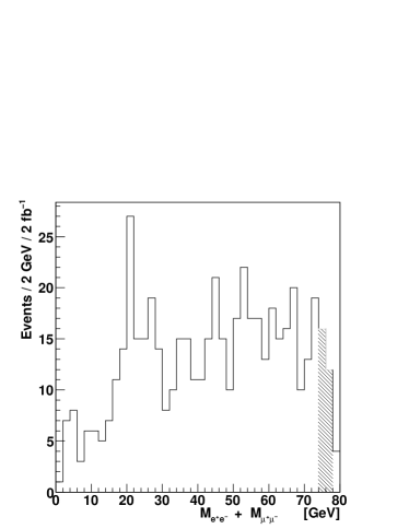
Figure 1: Events from the shaded bins of the OSSF distribution ($74~{}\mathrm{GeV}<M_{\ell\ell}<78~{}\mathrm{GeV}$) are used for DK analysis.

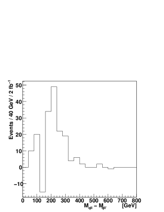
Figure 2: $M_{q\ell}$ and $M_{q\ell\ell}$ mass distributions, flavor-subtracted as described in the text and in Bachacou:1999zb . A rough estimate of the endpoints suffices for our analysis: $330~{}\mathrm{GeV}<\overline{M}_{q\ell\ell}<430~{}\mathrm{GeV}$, $300~{}\mathrm{GeV}<\overline{M}_{q\ell}<400~{}\mathrm{GeV}$.

To determine what set of SUSY masses is most consistent with this sample of events, we perform the following scan over mass space: $m_{s}$ is chosen in a liberal range, $100~{}\mathrm{GeV}<m_{s}<500~{}\mathrm{GeV}$ (lower bound from LEP constraints) as well as $\overline{M}_{q\ell\ell}$ and $\overline{M}_{q\ell}$ in ranges estimated from Fig.2, $300~{}\mathrm{GeV}<\overline{M}_{q\ell}<400~{}\mathrm{GeV}$, $330~{}\mathrm{GeV}<\overline{M}_{q\ell\ell}<430~{}\mathrm{GeV}$. Note that, as is customary in handling jet ambiguity, what we have actually plotted are the minimum values of $M_{q\ell\ell}$ and $M_{q\ell}$ computed from each of the two highest energy jets; also, before this minimization $M_{q\ell}$ is taken to be the larger of the two possible $q\ell$ masses. To reduce background and combinatorial effects further, these distributions are also computed for OSOF lepton events, labeled $M_{q\ell\ell^{\prime}}$ and $M_{q\ell^{\prime}}$, and are subtracted from the $M_{q\ell\ell}$ and $M_{q\ell}$ distributions, respectively. The total procedure thus improves endpoint precision at the cost of distorting distribution shape somewhat, but this is irrelevant to our present purpose.

For each choice of the endpoints $\overline{M}_{\ell\ell}$, $\overline{M}_{q\ell\ell}$ and $\overline{M}_{q\ell}$, the other unknown masses are then fixed from analytic expressions of the endpoints in terms of these masses and $m_{s}$ as

$$m_{1} = \sqrt{m_{s}^{2}-m_{s}\overline{M}_{\ell\ell}\sqrt{\overline{M}_{q\ell\ell}^{2}/\overline{M}_{q\ell}^{2}-1}},$$ (13)

$$m_{2} = m_{s}\sqrt{1+\overline{M}_{\ell\ell}^{2}/(m_{s}^{2}-m_{1}^{2})},$$ (14)

$$m_{\tilde{q}} = m_{2}\sqrt{1+\overline{M}_{q\ell\ell}^{2}/(m_{2}^{2}-m_{1}^{2})},$$ (15)

and for each such point in mass space the linear system of equations (7)–(11) is solved event-wise for $\not\!P_{n}$, constructing the sum (12) defining $\xi$. Both possible lepton assignments are tried. In this procedure each event contributes the minimum value of $|\sqrt{\not\!{P}_{n}^{2}}-m_{1}|$ resulting from matching the OSSF lepton pair to each of the two highest energy jets, accepting only solutions where the assumed lepton identity does indeed lead to reconstruction of the correct leptonic directions relative to the LSP momentum, i.e. the cosine of the angle between the assumed near(far) lepton momentum and the LSP must be $>\!\!(<)0$ in the rest frame of the decaying $\tilde{\chi}_{2}^{0}$. If, for any event $n$, the quantity $|\sqrt{\not\!{P}_{n}^{2}}-m_{1}|$ exceeds a tolerance $T$ (we take $T=30$ GeV), or if $\not\!{P}_{n}$ is tachyonic, or if the reconstruction of the $\tilde{\chi}_{2}^{0}$ velocity fails for both possible jet pairings, the event is assigned a fixed contribution of $T$ to $\xi$ (i.e. a fit which is $T=30$ GeV in error is deemed as bad as finding no fit at all). As with the $\epsilon$ parameter, $T$ is adjustable and could be optimized somewhat, but any reasonable value will do. The choice of $(m_{s},\overline{M}_{q\ell\ell},\overline{M}_{q\ell})$ giving the minimum $\xi$ is then assumed to yield the correct mass hypothesis. For the particular data set shown, we obtain $(m_{s},\overline{M}_{q\ell\ell},\overline{M}_{q\ell})=(133,408,300)$ GeV as the $\xi$-minimizing solution, and using (13)-(15) yields $(m_{1},m_{s},m_{2},m_{\tilde{q}})=(90.3,133.0,170.0,510.7)$ GeV, quite close to the nominal values of $(96,143,177,537)$ GeV.

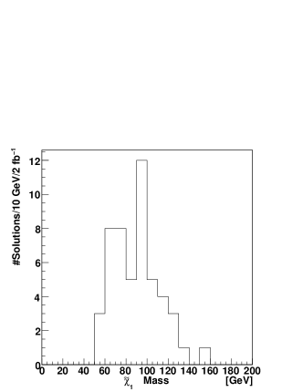
Figure 3: Best fits to the LSP mass for each of 50 independently-generated $2~{}\mathrm{fb}^{-1}$ data sets (SUSY signal + SM background).

To get some idea on the expected accuracy of this method owing to random fluctuations in signal and background, we look at the best-fit solutions in 50 independently-generated data sets, obtaining the following results:

$$m_{1} = ~{}89.9\pm 21.8~{}\mathrm{GeV}$$ (16)

$$m_{s} = 131.0\pm 22.2~{}\mathrm{GeV}$$

$$m_{2} = 169.2\pm 21.6~{}\mathrm{GeV}$$

$$m_{\tilde{q}} = 512.4\pm 31.4~{}\mathrm{GeV}$$

Quoted uncertainties are actually square-roots of sample variances. Though these results are slightly lower than the nominal values, one generally gets accurate (within $\sim 15-20\!$ %) estimates of the masses, and the spread in the solutions is consistent with the rough width of the peak in, for example, the LSP mass distribution in Fig. 3. This width scales with the jet energy-bias we put in by hand, so once low-luminosity jet reconstruction efficiency is better understood the accuracy of the method would be closer to $\sim 10-15$% on average.

Let us again stress that, prior to this Letter, the only known method of reconstructing particle masses in early-LHC data was the standard endpoint analysis, and this will give considerably worse results: in addition to the three endpoints $\overline{M}_{\ell\ell}$, $\overline{M}_{q\ell\ell}$, and $\overline{M}_{q\ell}$ whose precise determination is not possible with such low statistics, one needs a fourth endpoint, usually taken as the lower endpoint of the $M_{q\ell\ell}$ distribution, to solve for a point in $(m_{\tilde{q}},m_{2},m_{s},m_{1})$-space. However, this lower endpoint, which is supposed to be at ${M}_{q\ell\ell}=202$ GeV, is not discernible in Fig. 2. Studies with more sophisticated detector simulation and endpoint fitting algorithms point to uncertainties in the masses that can reach $50$% or more from early LHC dataLHCMET at comparable luminosities.

———————————————————

This Letter demonstrates that, in the early stages of the LHC, one may obtain far more accurate estimates of New Physics masses than previously thought if one uses a DK technique, at least for $\ell^{+}\ell^{-}j$ events assumed to arise from the squark cascade chain considered here. Generalization to the same final state arising from other models (such as extra dimensions or little higgs models), or to different decay topologies is straightforward. What makes DK so powerful in the present case is not only that one can utilize the high statistics in the dilepton endpoint, but that one can resolve lepton ambiguity through explicit reconstruction that does not rely on a measurement of MET. In fact, the same method may be used on a decay chain where the LSP decays through R-parity violating operators, as there is no reliance on pair-production of new sparticles. The need for an effective mass estimator in the early stages of the LHC is attractive not only to help theorists hone in on likely models for New Physics signals, but also in the design and optimization of experiments, especially with respects to the LSP, whose mass measurement at the LHC will directly affect designs of Dark Matter detection facilities elsewhere.

- (1) A.J. Barr and C.G. Lester, arXiv:1004.2732.
- (2) H. Bachacou, I. Hinchliffe, and F.E. Paige Phys. Rev. D 69, 015009 (2000).
- (3) B.K. Gjelsten, D.J. Miller, and P. Osland JHEP 12, 003 (2004).
- (4) C.G. Lester, and D.J. Summers, Phys. Lett. B 463, 99 (1999).
- (5) A. Barr C.G. Lester, and P. Stephens, J. Phys. G 29, 2343 (2003).
- (6) W.S. Cho, K. Choi, Y.G. Kim,and C.B. Park, Phys. Rev. Lett. 100, 171801 (2008).
- (7) K. Kawagoe M.M. Nojiri, and G. Polesello, Phys. Rev. D 71, 035008 (2005).
- (8) H.C. Cheng et al., JHEP 12, 076 (2007).
- (9) H.C. Cheng et al., Phys. Rev. Lett. 100, 252001 (2007).
- (10) G. Aad et al., (The ATLAS Collaboration) arXiv:0901.0512.
- (11) N. Kersting Phys. Rev. D 79, 095018 (2009).
- (12) Z. Kang, N. Kersting, S. Kraml, A. Raklev, and M. White arXiv:0908.1550.
- (13) B. Webber, JHEP 0909, 124 (2009).
- (14) B.C. Allanach et al., Eur.Phys.J. C25, 113 (2002).
- (15) T. Sjostrand, S. Mrenna, P. Skands, JHEP 05, 026 (2006).
- (16) E. Richter-Was, hep-ph/0207355.
- (17) G. Aad et al., (The ATLAS Collaboration), JINST 3, S08003 (2008).