Probabilistic Phase Space Trajectory Description for Anomalous Polymer Dynamics

Abstract

It has been recently shown that the phase space trajectories for the anomalous dynamics of a tagged monomer of a polymer — for single polymeric systems such as phantom Rouse, self-avoiding Rouse, Zimm, reptation, and translocation through a narrow pore in a membrane; as well as for many-polymeric system such as polymer melts in the entangled regime — is robustly described by the Generalized Langevin Equation (GLE). Here I show that the probability distribution of phase space trajectories for all these classical anomalous dynamics for single polymers is that of a fractional Brownian motion (fBm), while the dynamics for polymer melts between the entangled regime and the eventual diffusive regime exhibits small, but systematic deviations from that of a fBm.

In its terminal relaxation time $\tau$, $\tau\sim N^{\kappa}$, a polymer of length $N$ displaces itself in space by its own size, which itself scales as $\sim N^{\xi}$ degennes ; de . The values of $\kappa$ and $\xi$ vary from system to system. E.g., for phantom (self-intersecting) polymers $\xi=1/2$, and for self-avoiding polymers $\xi=\nu$, with $\nu=3/4$ in two and $\approx 0.588$ in three dimensions respectively. Similarly, for polymer dynamics in the absence of hydrodynamic interactions (Rouse: $\kappa=1+2\xi$ rouse ; kay ), and polymer dynamics in a good solvent (Zimm zimm ; degennes ; de : $\kappa=3\xi$). The above means, in the simplest case, that the mean-square displacement (MSD) of a tagged monomer of a polymer must behave $\sim t^{2\xi/\kappa}$ until time $\tau$, and $\sim t$ thereafter. Since $2\xi/\kappa$ is not necessarily unity, the dynamics of a tagged monomer in a polymer is anomalous till time $\tau$, and the polymer’s diffusion coefficient scales $\sim N^{2\xi-\kappa}$.

Starting from a microscopic description, there are two main approaches to model anomalous dynamics in stochastic systems rainer : (i) Continuous Time Random Walk (CTRW) mont and the associated fractional Fokker-Planck Equation (fFPE), providing a probabilistic description of phase-space trajectories, and (ii) the Generalized Langevin Equation (GLE) morikubozwan , which describes individual phase space trajectories. Physical systems exhibiting anomalous dynamics, for which probabilistic description of phase-space trajectories as well as description of individual trajectories can be obtained, are not only relatively rare, but also, relating one description to the other often requires approximations wang . Anyhow, given the ubiquity of anomalous dynamics in polymeric systems degennes ; de , one would expect them to have been thoroughly examined from this perspective. To the best of my knowledge however, probabilistic description of phase space trajectories for anomalous polymer dynamics has only been considered for isolated cases such as Rouse chain rouse1 , and polymer translocation metz ; vilgis ; kantor ; satya ; vocksa : in metz ; vilgis , an fFPE approach has been put forward, wherein, a (power-law) waiting time before each move of the monomer in the pore is assumed to cause the anomalous dynamics. This approach is at odds with numerical studies by others kantor , who report that, for the translocation of an infinite polymer, the probability distribution is Gaussian in space, but with a width that scales anomalously in time. Further, the anomalous dynamics of translocation has been shown to match that of the fractional Brownian motion (fBm) satya ; vocksa , which is also in contradiction with the fFPE approach.

As for the description of individual trajectories for anomalous polymer dynamics, two recent papers panja1 ; panja2 show that without external forces, the motion of a tagged monomer of a polymer — for phantom and self-avoiding Rouse, Zimm, reptation, translocation, and polymer melts — is robustly described by a unified Generalized Langevin Equation (GLE). The force $\vec{\phi}(t)$ experienced by the tagged monomer is related to its velocity $\vec{v}(t)$ via

polymeric system	derivation of Eq. (4) de	$\,\,\,\kappa\,\,\,$	$\gamma_{p}$	$k_{p}$
phantom Rouse	directly from Rouse equation	$2$	$\gamma_{0}=N\gamma$	$6\pi^{2}k_{B}Tp^{2}/N$
	no approximation		$\gamma_{p\neq 0}=2N\gamma$
Zimm (phantom) and	Smoluchowski equation; pre-averaging	$3/2$	$\,\,\,\gamma_{0}=3(6\pi^{3}N)^{1/2}\eta_{s}/8\,\,\,$	$6\pi^{2}k_{B}Tp^{2}/N$
polymer in a $\theta$-solvent	approximation on the mobility matrix		$\gamma_{p\neq 0}=(12\pi^{3}Np)^{1/2}\eta_{s}$
Zimm (self-avoiding)	Smoluchowski equation; pre-averaging	$3\nu$	$\gamma_{0}=\eta_{s}N^{\nu}$	$\,\,\,N^{-2\nu}k_{B}Tp^{1+2\nu}\,\,\,$
	approximation on the mobility matrix		$\gamma_{p}=\eta_{s}N^{\nu}p^{1-\nu}$
reptation	entropic (curvilinear) chain tension;	$2$	$\gamma_{0}=N\gamma$	$6\pi^{2}k_{B}Tp^{2}/N$
(curvilinear co-ordinate)	i.e., Eq. (4) is only one-dimensional		$\gamma_{p\neq 0}=2N\gamma$

Table 1: Elaboration of Eq. (4) for phantom Rouse, Zimm, polymer in a $\theta$-solvent and reptation. Here $\eta_{s}$ is the solvent viscosity. Where applicable, the effective damping coefficient $\gamma$ for monomeric motion, as defined in Eq. (2), is $\propto\eta_{s}$. Note, in all cases, that $\kappa$ is simply the power of $p$ in the expression $k_{p}/\gamma_{p}$ for $p\neq 0$.

$$\vec{\phi}(t)=-\int_{0}^{t}dt^{\prime}\mu(t-t^{\prime})\vec{v}(t^{\prime})+\vec{g}(t),$$ (1)

where $\mu(t)$ is the memory kernel, and the noise $\vec{g}(t)$ satisfies $\langle\vec{g}(t)\rangle_{0}=0$ and the fluctuation-dissipation theorem (FDT) $\langle g_{\sigma}(t)g_{\lambda}(t^{\prime})\rangle_{0}=k_{B}T\delta_{\sigma\lambda}\mu(t-t^{\prime})$, with $\sigma,\lambda=(x,y,z)$. Here $\langle\ldots\rangle_{0}$ denotes an average over the noise realizations, including an average over equilibrium configurations of the polymers at $t=0^{-}$. Further, with $\vec{v}(t)$ responding to $\vec{\phi}(t)$ as $\gamma\vec{v}(t)=\vec{\phi}(t)+\vec{f}(t)$, where $\gamma$ is the (effective) damping coefficient for monomeric motion, and $\vec{f}(t)$ is a random force satisfying $\langle\vec{f}(t)\rangle=0$ and the FDT $\langle f_{\sigma}(t)f_{\lambda}(t^{\prime})\rangle=2\gamma k_{B}T\delta_{\sigma\lambda}\delta(t-t^{\prime})$, one has

$$\vec{v}(t)=\gamma^{-1}\left[-\int_{0}^{t}dt^{\prime}\mu(t-t^{\prime})\vec{v}(t^{\prime})+\vec{g}(t)+\vec{f}(t)\right].$$ (2)

In this formulation, $\mu(t)\sim t^{-\alpha}e^{-t/\tau}$ for some $0<\alpha<1$ (for a list, see Table I of panja2 ). The FDT then ensures that the MSD $\sim t^{\alpha}$ till time $\tau$, and $\sim t$ thereafter. This formulation also robustly yields the correct drift behavior of a tagged monomer under weak external forces panja2 , like the Nernst-Einstein relation. The GLE (1-2), describing non-Markovian trajectories in phase space, demonstrate that there is no power-law waiting time (assumed in the modeling of translocation by the fFPE); instead, the anomalous dynamics stems from the fact that each move of the tagged monomer tends to be undone later.

Here I demonstrate that, with a $\delta$-function distribution in 3D space at $t=0$, the probability distribution of a tagged monomer for phantom Rouse, self-avoiding Rouse, Zimm, polymers in a $\theta$-solvent, reptation, translocation, and polymer melts in the entangled regime is given by

$$P(\vec{r},t|\vec{r}_{0},0)=e^{-(\vec{r}-\vec{r}_{0})^{2}/2\Delta(t)}/[2\pi\Delta(t)]^{3/2},$$ (3)

with $\Delta(t)=At^{\alpha}e^{-t/\tau}+BN^{2\xi-\kappa}t$, where $A$ and $B$ are two system parameters-dependent constants, and $N^{2\xi-\kappa}$ is the scaling of the polymer’s diffusion coefficient with $N$ [for translocation, Eq. (3) holds only until the polymer disengages from the pore; see later]; i.e., the anomalous dynamics of an infinite polymer is that of the fBm mandel . One should keep in mind that Eq. (3) is demonstrated here for polymeric systems wherein the polymers are far away from any boundary (including translocation), as Eq. (3) cannot be reconciled with nontrivial boundary conditions. The GLE (1-2) and Eq. (3) thus provide a complete description (i.e., of individual trajectories as well as that of trajectory distribution in phase space) of anomalous dynamics in polymeric systems; as mentioned earlier, this is relatively rare for physical systems.

In fact, $P(\vec{r},t|\vec{r}_{0},0)$ for phantom Rouse, Zimm, polymers in a $\theta$-solvent, and reptation can be obtained analytically, irrespective of the GLE description, thanks to the fact that their dynamics is described by that of the polymer’s fluctuation modes. For these systems, the location $\vec{R}_{n}(t)$ of monomer $n$ can be expressed, in terms of the mode amplitude $\{\vec{X}_{p}(t)\}$s for $p=0,1,2\ldots$, as $\vec{R}_{n}(t)=\vec{X}_{0}(t)+\sum_{p=1}^{\infty}\vec{X}_{p}(t)\cos(\pi pn/N)$, obeying the boundary condition that the polymer’s chain tension vanishes at the free ends, i.e., $[\partial\vec{R}_{n}(t)/\partial n]_{n=0}=[\partial\vec{R}_{n}(t)/\partial n]_{n=N}=0$. As the $\{\vec{X}_{p}(t)\}$s can be obtained by an inverse cosine transformation of the above, the polymer dynamics is simply reconstructed from the LE satisfied by each spatial component (denoted by $\sigma$) of the $\{\vec{X}_{p}(t)\}$s de

$$\gamma_{p}\dot{X}_{p\sigma}(t)=-k_{p}X_{p\sigma}(t)+f_{p\sigma}(t),$$ (4)

where the stochastic force satisfies $\langle f_{p\sigma}(t)\rangle=0$ and the FDT $\langle f_{p\sigma}f_{q\lambda}\rangle=2\gamma_{p}k_{B}T\delta_{\sigma\lambda}\delta_{pq}\delta(t-t^{\prime})$. The list of $\gamma_{p}$ and $\kappa_{p}$ values for these systems appear in Table 1: note that the relaxation time $\tau_{p}$ for the $p$-th mode $\tau_{p}=\gamma_{p}/k_{p}=c^{-1}p^{-\kappa}$ for $p\neq 0$; one can calculate $c$ from the table.

polymeric system	$\Delta(t)$
phantom Rouse	$\sim t^{1/2}$ till $\tau$ and $\sim t$ thereafter
Zimm (phantom) and	$\sim t^{2/3}$ till $\tau$ and $\sim t$ thereafter
polymer in a $\theta$-solvent
Zimm (self-avoiding)	$\sim t^{2/3}$ till $\tau$ and $\sim t$ thereafter
reptation	$\sim t^{1/2}$ till $\tau$ and $\sim t$ thereafter
(curvilinear co-ordinate)
self-avoiding Rouse	$\sim t^{\frac{2\nu}{1+2\nu}}$ till $\tau$ and $\sim t$ thereafter

Table 2: Systems of Table 1 and their $\Delta(t)$-behavior. Note that the scaling exponent of $\Delta(t)$ with time, in each case, is given by $2\xi/\kappa$, as noted in the first paragraph of the paper.

With the above, $P(\vec{r},t|\vec{r}_{0},0)$ is calculated as follows. For fixed $\{\vec{X}_{p}^{(0)}\}$s that correspond to the position $\vec{r}_{0}$ of the tagged monomer at $t=0$, one determines the probability ${\cal P}(\vec{X}_{p},t|\vec{X}_{p}^{(0)},0)$ from Eq. (4). One then obtains $P(\vec{r},t|\vec{r}_{0},0)$ by integrating over all values of $\{X_{p}(t)\}$ that correspond to the position $\vec{r}$ of the tagged monomer at time $t$, taking into account the equilibrium distribution of the $\{\vec{X}_{p}^{(0)}\}$-values. With the tagged monomer being the middle monomer, this calculation, demonstrating Eq. (3) for phantom Rouse, Zimm, polymers in a $\theta$-solvent, and reptation are detailed in Appendix A: therein it is seen that [c.f. Eqs. (A13-A17)]

$$\Delta(t)\sim\int_{0}^{\infty}\frac{dp}{k_{p}}\,\left(1-e^{-t/\tau_{p}}\right),$$ (5)

i.e., the exponent of $\Delta(t)$ in time is determined by the integral in Eq. (5). The corresponding scalings of $\Delta(t)$ summarized in Table 2. Further, based on prouse , I note that one can construct an effective Eq. (4) also for self-avoiding polymers, with $p$-independent $\gamma_{0}$ and $\gamma_{p\neq 0}$, and $k_{p}\sim p^{1+2\nu}$. The corresponding scaling behavior for $\Delta(t)$, also calculated in Appendix A, is listed in Table 2, and is verified by simulations in Fig. 1.

It is interesting to note here that the mode expansion technique to establish Eq. (3) for the systems of Table 1 implies that Eq. (3) is a simple consequence of the physical connectivity of the polymer chain.

The expansion of the monomer co-ordinates into polymer’s fluctuation modes also provides an insight into how, given the GLE (1-2), one may expect $P(\vec{r},t|\vec{r}_{0},0)$ to be Gaussian. E.g., consider an ensemble ${\cal E}$ of polymers, at equilibrium at $t=0^{-}$, with a given velocity history of the middle monomer between times $0$ and $t$. For this ensemble, if $[\vec{g}(t)+\vec{f}(t)]$ can be shown to be Gaussian, then the displacements of the middle monomer in an infinitesimal time between $t$ and $(t+dt)$ is Gaussian distributed about the mean $-\gamma^{-1}\int_{0}^{t}dt^{\prime}\mu(t-t^{\prime})\vec{v}(t^{\prime})$, since $\vec{v}(t)$ is proportional to $[\vec{g}(t)+\vec{f}(t)]$. Such (infinitesimal) Gaussian displacements, accumulated over time, would then mean that $P(r_{\sigma},t|r_{\sigma 0},0)$ has to be Gaussian.

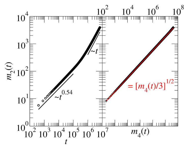
Figure 1: (color online) Equation (3) for self-avoiding Rouse polymers ($N=400$): model details can be found in Appendix B. Left: second moment $m_{2}(t)=\sum_{\sigma}\langle[r_{\sigma}(t)-r_{\sigma}(0)]^{2}\rangle/3$ of the distribution (3), scales as $t^{\frac{2\nu}{1+2\nu}}\sim t^{0.54}$ till $\tau$, and $\sim t$ thereafter. Right: $m_{2}(t)$ against $m_{4}(t)=\sum_{\sigma}\langle[r_{\sigma}(t)-r_{\sigma}(0)]^{4}\rangle/3$. Red line: $m_{2}(t)=[m_{4}(t)/3]^{1/2}$ — note that $m_{4}(t)=3[m_{2}(t)]^{2}$ for a Gaussian distribution. Data obtained from a time-series of 200,000 consecutive snapshots, separated by 400 time units each, of 256 different polymers.

In order to mathematically appreciate the Gaussian behavior of $[\vec{g}(t)+\vec{f}(t)]$, one needs to recall the physics behind the anomalous dynamics for these systems panja1 ; panja2 : a move of the middle monomer creates a local strain by altering the polymer’s chain tension locally [Eq. (1)]. In response to this strain, in subsequent times there is an enhanced chance, for the monomer, to undo the move [Eq. (2)]. This physics is best represented by discretizing the movement of the middle monomer in time for the ensemble ${\cal E}$ panja2 ; e.g., $v(t)=\sum_{i=0}^{m}\delta\vec{r}_{i}\delta(t-t_{i})$ for some $m$, and $t_{0}=0$ by choice. In between these moves the middle monomer remains stationary, i.e., the dynamics of the polymer is given by those of the mode amplitudes $\{\vec{Y}_{p}(t)\}$s, with the monomer locations $\vec{r}_{n}(t)$ relative to the middle monomer expressed as $\vec{r}_{n}(t)=4\sum_{p}\vec{Y}^{(r)}_{p}(t)\sin\frac{\pi(2p+1)n}{N}\,\Theta(n-N/2)-4\sum_{p}\vec{Y}^{(l)}_{p}(t)\sin\frac{\pi(2p+1)n}{N}\,\Theta(N/2-n)$ for $p=0,1,2,\ldots$ (the superscripts for $\vec{Y}(t)$ correspond to the right and the left halves of the polymer). The $\{Y_{p}(t)\}$s are obtained from $\{\vec{r}_{n}(t)\}$s via the inverse sine transform, and are readily shown to satisfy the boundary condition that the chain tension vanishes at the open ends of the polymer. Through this formulation, the polymer’s chain tension at the middle monomer, expressed in terms of the $\{\vec{Y}_{p}(t)\}$s, changes discretely at $\{t_{i}\}$s, while in between, the relaxation of the chain tension gives rise to the memory kernel of Eq. (1). To work this out for all systems of Table 1, one needs to re-perform, as applicable, the pre-averaging approximation in terms of the $\{\vec{Y}_{p}(t)\}$s, which is a cumbersome task. For the sake of simplicity, I therefore only consider the phantom Rouse case here; for this system, in times $t_{i}<t<t_{i+1}$, the $\{\vec{Y}_{p}(t)\}$s for each half independently obey the LE panja2

$$\gamma_{p}\frac{\partial\vec{Y}_{p}}{\partial t}=-q_{p}\,\vec{Y}_{p}(t)+\vec{h}_{p}(t),$$ (6)

with $\gamma_{p}=2N\gamma$, $q_{p}=6\pi^{2}k_{B}T(2p+1)^{2}/N$, $\tau_{2p+1}=\gamma_{p}/q_{p}$, $\langle\vec{h}_{p}\rangle=0$ and $\langle h_{p\sigma}(t)h_{q\lambda}(t^{\prime})\rangle=\gamma_{p}k_{B}T\delta(t-t^{\prime})\delta_{pq}\delta_{\sigma\lambda}$. Then $\vec{g}(t)$ in Eq. (1-2) is given by (see Eq. (19) of panja2 )

$$\vec{g}(t)=4\sum_{p}\!\frac{\pi(2p+1)}{N}\Bigg{\{}\!e^{-t/\tau_{2p+1}}[\vec{Y}^{(r)}_{p}(0^{-})+\vec{Y}^{(l)}_{p}(0^{-})]$$ (7)

$$+\frac{1}{\gamma}_{p}\int_{0}^{t}\!\!dt^{\prime}\,e^{-(t-t^{\prime})/\tau_{2p+1}}[\vec{h}^{(r)}_{p}(t^{\prime})+\vec{h}^{(l)}_{p}(t^{\prime})]\Bigg{\}}.$$

With $\vec{f}(t)$, $\{\vec{h}_{p}(t)\}$s, $\{\vec{Y}_{p}(0^{-})\}$s being Gaussian distributed with zero mean [as of Eqs. (2) and (7) respectively], $[\vec{g}(t)+\vec{f}(t)]$ also has to be Gaussian.

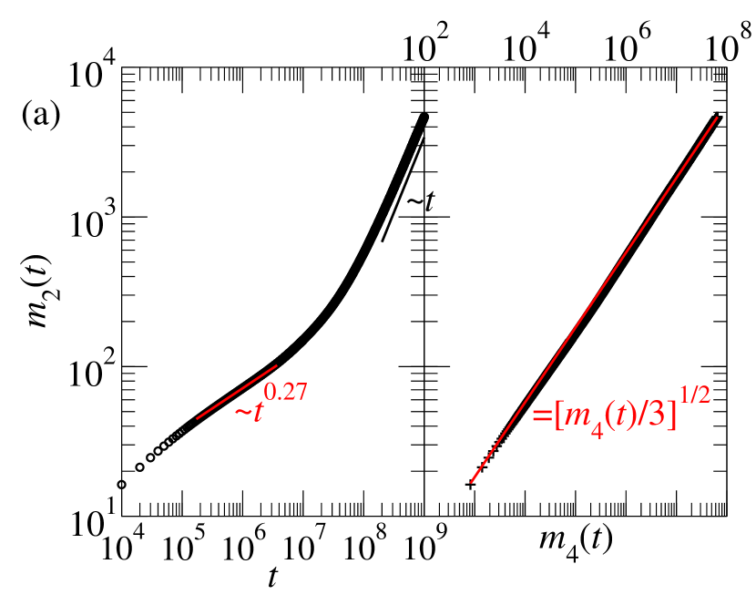
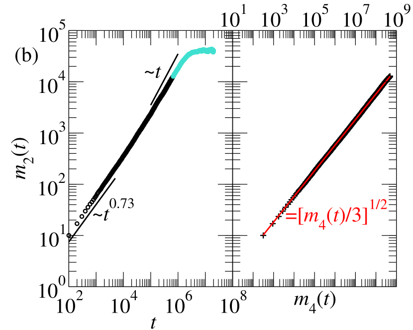
Figure 2: (color online) (a) Left: The second moment $m_{2}(t)=(1/3)\sum_{\sigma}\langle[r_{\sigma}(t)-r_{\sigma}(0)]^{2}\rangle$ of the distribution (3) for the middle monomer of a tagged polymer in a melt. Right: $m_{2}(t)$ against $m_{4}(t)=(1/3)\sum_{\sigma}\langle[r_{\sigma}(t)-r_{\sigma}(0)]^{4}\rangle$; red line: $m_{2}(t)=[m_{4}(t)/3]^{1/2}$. Data obtained from long time-series of 155,000 consecutive snapshots, separated by $10^{4}$ time units each, of 1,728 different polymers with $N=1500$. See text for graph description. (b) Left: The second moment $m_{2}(t)=[s(t)-N/2]^{2}$, where $s(t)$ is the monomer number threaded in the pore at time $t$, $s(0)=N/2$. Right: $m_{2}(t)$ against $m_{4}(t)=\langle[s(t)-N/2]^{4}\rangle$; red line: $m_{2}(t)=[m_{4}(t)/3]^{1/2}$. Data averaged over 8,192 different polymers of $N=1000$, for the turquoise points in the left graph at least one polymer of the 8,192 polymers has disengaged from the pore. See text for graph descriptions.

Thus, to summarize so far, having expanded the monomer co-ordinates in polymer’s fluctuation modes, I have shown that $P(\vec{r},t|\vec{r}_{0},0)$ for phantom Rouse, Zimm, polymers in a $\theta$-solvent, reptation and self-avoiding Rouse is Gaussian; and have illustrated, for the specific case of phantom Rouse, that Gaussianity of $P(\vec{r},t|\vec{r}_{0},0)$ is expected from the GLE (1-2) since the noise term $[\vec{g}(t)+\vec{f}(t)]$ is Gaussian. Unfortunately however, the mode expansion does not work as simply for translocation (for which, the tagged monomer is the one within the pore at time $t$, i.e., it does not even have a fixed index) and for polymer melt. Neither can Gaussianity of $[\vec{g}(t)+\vec{f}(t)]$ be shown, and therefore, one has to rely on computer simulations. The data for the melt are presented in Fig. 2(a): simulations are performed at overall monomer density unity; the simulation details, same as that of panja2 where the GLE has been shown to describe the dynamics of the middle monomer of a tagged polymer in the entangled regime, can be found in Appendix B. Following reptation theory for polymer melts, one expects the second moment $m_{2}(t)$ to behave $\sim t^{1/4}$ in the entangled regime, which starts around time $\sim 10^{5}$ for this model; in this regime an effective exponent 0.27 is found (the red line in the left graph). While the right graph is consistent with Eq. (3) in the entangled regime, between the entangled regime and the eventual diffusive regime, $P(\vec{r},t|\vec{r}_{0},0)$ does deviate very slightly, and systematically, from (3), indicating that the noise term $[\vec{g}(t)+\vec{f}(t)]$ is not Gaussian during this time.

The data for unbiased translocation are presented in Fig. 2(b) [see model details in Appendix B]. The monomer number within the pore at time $t$ is denoted by $s(t)$. Polymers are equilibrated with $s(0)=N/2$. Here $m_{2}(t)\sim t^{(1+\nu)(1+2\nu)}\approx t^{0.73}$, and should cross over to diffusive behavior, as predicted in anom , although the crossover is slow: at long times polymers start disengaging from the pore, corresponding to the flattening of $m_{2}(t)$ (the turquoise points in the left graph), hence the true diffusive behavior can only be observed for very long polymers. Nevertheless, Eq. (3) is verified cleanly up to the point when all polymers remain threaded in the pore: this behavior is in agreement with kantor ; satya [albeit they report an anomalous exponent different from $(1+\nu)/(1+2\nu)$], and contradicts vilgis , reaffirming that fFPE is not applicable for polymer translocation.

Finally, I note that the drift of a tagged monomer due to a weak external force $\vec{F}$ (i.e., in the linear response regime), is given by $t^{\alpha}\vec{F}$ till time $\tau$ and $t\vec{F}$ thereafter, where $\alpha$ is the anomalous exponent. Describing this requires a simple extension of Eq. (3).

Ample computer time from the Dutch national supercomputer facility SARA, and help from Gerard Barkema with simulations are gratefully acknowledged. It is also a pleasure to thank Gerard Barkema and Rainer Klages for helpful comments on the manuscript.

Appendix A Appendix A: : Derivation of Eq. (3) for the middle monomer for phantom Rouse, Zimm, polymers in a $\theta$-solvent, reptation, and self-avoiding Rouse polymers

I tag the middle monomer of the polymer, and here I obtain Eq. (3) for its dynamics.

I start with the Langevin equation (3) describing the evolution of the $p$-th mode amplitude ($p=0,1,2,\ldots$), viz.,

$$\gamma_{p}\frac{X_{p\sigma}(t)}{\partial t}=-k_{p}X_{p\sigma}(t)+f_{p\sigma}(t)\,,$$ (A1)

with $\langle f_{p\sigma}\rangle=0$ and the FDT $\langle f_{p\sigma}(t)f_{q\lambda}(t^{\prime})\rangle=2\gamma_{p}k_{B}T\delta(t-t^{\prime})\delta_{pq}\delta_{\sigma\lambda}$. As noted in Table 1, Eq. (A1) can be derived for phantom Rouse, Zimm, polymers in a $\theta$-solvent and reptation. A straightforward result that follows from Eq. (A1) is that

$$\langle X_{p\sigma}(t)X_{q\lambda}(t^{\prime})\rangle=\delta_{pq}\delta_{\sigma\lambda}(k_{B}T/k_{p})e^{-k_{p}(t-t^{\prime})/\gamma_{p}}=\delta_{pq}\delta_{\sigma\lambda}(k_{B}T/k_{p})e^{-(t-t^{\prime})/\tau_{p}},$$ (A2)

where $\tau_{p}$ is the relaxation time of the $p$-th mode ($p\neq 0$) for the polymer. When Eq. (A2) is combined with the corresponding time correlation function for mode amplitudes for self-avoiding polymers prouse , namely $\langle\vec{X}_{p}(t)\cdot\vec{X}_{q}(t^{\prime})\rangle\propto N^{2\nu}p^{-(1+2\nu)}e^{-t/\tau_{p}}\delta_{pq}$ with $\tau_{p}\sim(N/p)^{1+2\nu}$, one can formulate an effective Eq. (4) with both $\gamma_{0}$ and $\gamma_{p\neq 0}$ independent of $p$, and $k_{p}\sim p^{-(1+2\nu)}$ [this implies that for a self avoiding polymer $\tau_{p}\sim(N/p)^{1+2\nu}$]. Given this, I will henceforth use Eq. (A1) also for self-avoiding Rouse polymers.

The Fokker-Planck equation for the probability ${\cal P}(X_{p\sigma},t)$ that corresponds to the LE is given by vankampen

$$\frac{\partial{\cal P}(X_{p\sigma},t)}{\partial t}=\underbrace{\frac{k_{p}}{\gamma_{p}}}_{=\tau^{-1}_{p}\,\,\mbox{for}\,\,p\neq 0}\frac{\partial}{\partial X_{p\sigma}}\left[X_{p\sigma}{\cal P}(X_{p\sigma},t)\right]+\underbrace{\frac{k_{B}T}{\gamma_{p}}}_{=a_{p}\tau^{-1}_{p}\,\,\mbox{for}\,\,p\neq 0}\frac{\partial^{2}{\cal P}(X_{p\sigma},t)}{\partial X^{2}_{p\sigma}},$$ (A3)

where $a_{p}=k_{B}T/k_{p}$ for $p\neq 0$, and $a_{0}=k_{B}T/\gamma_{0}$. The solution of Eq. (A3), with the initial condition that $P(X_{p\sigma},0)=\delta(X_{p\sigma}-X^{(0)}_{p\sigma})$, is obtained as follows.

• For $p=0$, $k_{p}=0$ i.e., (A3) is a simple diffusion equation. Its solution is given by uh

  $${\cal P}(X_{0\sigma},t)=\frac{1}{\sqrt{2\pi a_{0}t}}\,\exp\left[-\frac{(X_{0\sigma}-X^{(0)}_{0\sigma})^{2}}{2a_{0}t}\right].$$ (A4)

• For $p\neq 0$, Eq. (A3) can be verified by direct substitution of its solution

  $${\cal P}(X_{p\sigma},t)=\frac{1}{\sqrt{2\pi a_{p}(1-e^{-2t/\tau_{p}})}}\,\exp\left[-\frac{(X_{p\sigma}-X^{(0)}_{p\sigma}e^{-t/\tau_{p}})^{2}}{2a_{p}(1-e^{-2t/\tau_{p}})}\right].$$ (A5)

Next, as noted above Eq. (4), in terms of the mode amplitudes, the location of the middle monomer ($n=N/2$) at any time $t$ is given by

$$\vec{r}(t)=\vec{X}_{0}(t)+2\sum_{p=1}^{\infty}\vec{X}_{p}(t)\,\cos\frac{p\pi}{2}.$$ (A6)

Using Eq. (A6), I obtain, upon averaging over all possible initial states of the polymer at $t=0$

$$P(r_{\sigma},t|r_{0\sigma},0)=\prod_{p=0}^{\infty}\int_{-\infty}^{\infty}dX^{(0)}_{p\sigma}\,{\cal P}_{\text{eq}}(X^{(0)}_{p\sigma})\,\,\delta\!\!\left[r_{0\sigma}-\left(X^{(0)}_{0\sigma}+2\sum_{q=1}^{\infty}X^{(0)}_{q\sigma}\,\cos\frac{q\pi}{2}\right)\right]$$ (A7)

$$\times\int_{-\infty}^{\infty}dX_{p\sigma}\,{\cal P}(X_{p\sigma},t)\,\,\delta\!\!\left[r_{\sigma}-\left(X_{0\sigma}+2\sum_{q=1}^{\infty}X_{q\sigma}\,\cos\frac{q\pi}{2}\right)\right],$$

where ${\cal P}_{\text{eq}}(X)$ is the equilibrium probability of $X$, i.e., a Gaussian, obtained by taking the $t\rightarrow\infty$ limit of Eq. (A5).

At this stage, because of the $\delta$-functions in Eq. (A7), it is easiest to Fourier transform $P(r_{\sigma},t|r_{0\sigma},0)$, defined as

$$\tilde{\cal P}_{k,k^{\prime};t}=\frac{1}{2\pi}\int dr_{\sigma}\,dr_{0\sigma}e^{i\left[k^{\prime}r_{\sigma}+kr_{0\sigma}\right]}\,{\cal P}(r_{\sigma},t|r_{0\sigma},0],$$ (A8)

which reduces Eq. (A7) to

$$2\pi\,e^{-i\left[kr_{\sigma}+k^{\prime}r_{0\sigma}\right]}\tilde{\cal P}_{k,k^{\prime};t}=\prod_{p=0}^{\infty}\int_{-\infty}^{\infty}dX^{(0)}_{p\sigma}\,{\cal P}_{\text{eq}}(X^{(0)}_{p\sigma})\,e^{-ik\left[X^{(0)}_{0\sigma}+2\sum_{q=1}^{\infty}X^{(0)}_{q\sigma}\,\cos\frac{q\pi}{2}\right]}$$ (A9)

$$\times\int_{-\infty}^{\infty}dX_{p\sigma}\,{\cal P}(X_{p\sigma},t)\,e^{-ik^{\prime}\left[X_{0\sigma}+2\sum_{q=1}^{\infty}X_{q\sigma}\,\cos\frac{q\pi}{2}\right]},$$

At this point, in order to follow through the calculation of $\tilde{\cal P}_{k,k^{\prime};t}$, I need the two following integrals:

• $$\int_{-\infty}^{\infty}dX_{0\sigma}\,\frac{1}{\sqrt{2\pi a_{0}t}}\,\exp\left[-\frac{(X_{0\sigma}-X^{(0)}_{0\sigma})^{2}}{2a_{0}t}-ik^{\prime}X_{0\sigma}\right]=e^{-iX^{(0)}_{0\sigma}k^{\prime}-\frac{1}{2}a_{0}tk^{\prime 2}}.$$ (A10)

• for $p\neq 0$:

  $$\int_{-\infty}^{\infty}dX_{p\sigma}\,\frac{1}{\sqrt{2\pi a_{p}(1-e^{-2t/\tau_{p}})}}\,\exp\left[-\frac{(X_{p\sigma}-X^{(0)}_{p\sigma}e^{-t/\tau_{p}})^{2}}{2a_{p}(1-e^{-2t/\tau_{p}})}-2ik^{\prime}X_{p\sigma}\cos\frac{p\pi}{2}\right]$$ (A11)

  $$=e^{-2iX^{(0)}_{p\sigma}e^{-t/\tau_{p}}k^{\prime}\cos(p\pi/2)-2a_{p}(1-e^{-2t/\tau_{p}})k^{\prime 2}\cos^{2}(p\pi/2)}.$$

Using (a-b), I now integrate over $X^{(0)}_{0\sigma}$ (i.e., the location the center-of-mass of the polymer) with a uniform probability density measure yields $\sqrt{2\pi}\delta(k+k^{\prime})$, which leads me to

$$\sqrt{2\pi}\,e^{-i\left[k^{\prime}r_{\sigma}+kr_{0\sigma}\right]}\tilde{\cal P}_{k,k^{\prime};t}=e^{-k^{2}\left[\frac{1}{2}a_{0}t+2\sum_{q=1}^{\infty}a_{q}(1-e^{-2t/\tau_{q}})\cos^{2}(q\pi/2)\right]}\delta(k+k^{\prime})$$ (A12)

$$\times\prod_{p=1}^{\infty}\!\!\left[\int_{-\infty}^{\infty}\!\!\!\!\!dX^{(0)}_{p\sigma}\,{\cal P}_{\text{eq}}(X^{(0)}_{p\sigma})e^{-2ik\left[X^{(0)}_{p\sigma}(1-e^{-t/\tau_{p}})\cos(p\pi/2)\right]}\right]$$

$$=e^{-k^{2}\left[\frac{1}{2}a_{0}t+2\sum_{q=1}^{\infty}a_{q}\cos^{2}(q\pi/2)\{(1-e^{-2t/\tau_{q}})+(1-e^{-t/\tau_{q}})^{2}\}\right]}\delta(k+k^{\prime})$$

$$=e^{-k^{2}\left[\frac{1}{2}a_{0}t+4\sum_{q=1}^{\infty}a_{q}\cos^{2}(q\pi/2)(1-e^{-t/\tau_{q}})\right]}\delta(k+k^{\prime});$$

${\cal P}_{k,k^{\prime};t}\propto\delta(k+k^{\prime})$ implies that $P(r_{\sigma},t|r_{0\sigma},0)$ is a function of $(r_{\sigma}-r_{0\sigma})$.

Finally, I now need to evaluate the discrete sum in the exponent of Eq. (A12). Having noticed that $\cos(q\pi/2)=0$ for odd $q$-values and $\cos^{2}(q\pi/2)=1$ for even $q$-values, the sum can be converted into an integral; thereafter the inverse Fourier transform from $k$ to $(r_{\sigma}-r_{0\sigma})$ leads to Eq. (3), with the behavior of $\Delta(t)$ presented in Table 2. With the corresponding scaling of $\gamma_{p}$ and $\tau_{p}=\gamma_{p}/k_{p}$ for phantom Rouse, Zimm, polymers in a $\theta$-solvent, reptation, and self-avoiding Rouse polymers (see Table 1), these integrals are listed below. Note that in Eqs. (A13-A17) I omit constants in converting the discrete sums to integrals.

• Phantom Rouse:

  $$4\sum_{q=1}^{\infty}a_{q}\cos^{2}(q\pi/2)(1-e^{-t/\tau_{q}})\rightarrow k_{B}T\int_{0}^{\infty}\frac{dq}{q^{2}}\,(1-e^{-cq^{2}t})\sim\sqrt{t}.$$ (A13)

• Phantom Zimm and polymers in a $\theta$-solvent:

  $$4\sum_{q=1}^{\infty}a_{q}\cos^{2}(q\pi/2)(1-e^{-t/\tau_{q}})\rightarrow k_{B}T\int_{0}^{\infty}\frac{dq}{q^{2}}\,(1-e^{-cq^{3/2}t})\sim t^{2/3}.$$ (A14)

• (self-avoiding) Zimm:

  $$4\sum_{q=1}^{\infty}a_{q}\cos^{2}(q\pi/2)(1-e^{-t/\tau_{q}})\rightarrow k_{B}T\int_{0}^{\infty}\frac{dq}{q^{1+2\nu}}\,(1-e^{-cq^{3\nu}t})\sim t^{2/3}.$$ (A15)

• reptation (curvilinear co-ordinate):

  $$4\sum_{q=1}^{\infty}a_{q}\cos^{2}(q\pi/2)(1-e^{-t/\tau_{q}})\rightarrow k_{B}T\int_{0}^{\infty}\frac{dq}{q^{2}}\,(1-e^{-cq^{2}t})\sim\sqrt{t}.$$ (A16)

• self-avoiding Rouse:

  $$4\sum_{q=1}^{\infty}a_{q}\cos^{2}(q\pi/2)(1-e^{-t/\tau_{q}})\rightarrow k_{B}T\int_{0}^{\infty}\frac{dq}{q^{1+2\nu}}\,(1-e^{-cq^{1+2\nu}t})\sim t^{2\nu/(1+2\nu)}.$$ (A17)

Clearly, these power-law behavior of $\Delta(t)$ cannot hold longer than time $\tau$, this is also noted in Table 2.

Appendix B Appendix B: Simulation details

Over the past years, a highly efficient simulation approach to polymer dynamics has been developed in our group. This is made possible via a lattice polymer model, based on Rubinstein’s repton model rub for a single reptating polymer, with the addition of sideways moves (Rouse dynamics). A detailed description of this model, its computationally efficient implementation and a study of some of its properties and applications can be found in heuk1 .

In this model, each polymer is represented by a sequential string of monomers, living on a face-centered-cubic lattice with periodic boundary conditions in all three spatial directions. Hydrodynamic interactions between the monomers are not taken into account in this model. Monomers adjacent in the string are located either in the same, or in neighboring lattice sites. The polymers are self-avoiding: multiple occupation of lattice sites is not allowed, except for a set of adjacent monomers. The number of stored lengths within any given lattice site is one less than the number of monomers occupying that site. The polymers move through a sequence of random single-monomer hops to neighboring lattice sites. These hops can be along the contour of the polymer, thus explicitly providing reptation dynamics. They can also change the contour “sideways”, providing Rouse dynamics. Each kind of movement is attempted with a statistical rate of unity, which defines the unit of time. This model has been used before to simulate the diffusion and exchange of polymers in an equilibrated layer of adsorbed polymers wolt1 , dynamics self-avoiding Rouse polymers prouse1 , polymer translocation under a variety of circumstances vocksa ; anom ; panjatrans , and the dynamics of polymer adsorption adsorb .

The same model has been used for the polymer melt simulations (here the polymers are both self- and mutually-avoiding) for a system of size $60^{3}$ with an overall monomer density unity per lattice site. Due to the possibility that adjacent monomers belonging to the same polymer can occupy the same site, overall approximately 40% of the sites typically remain empty.

Initial thermalizations were performed as follows: completely crumpled up polymers are placed in lattice sites at random. The system is then brought to equilibrium by letting it evolve up to $10^{9}$ units of time, with a combination of random intermediate redistribution of stored lengths within each polymer. Additional details on the melt simulations can be found in panja2 .

References

(1) De Gennes P-G, 1985 Scaling concepts in polymer
physics (Ithaca, Cornell, revised edition).
(2) Doi M and Edwards S F, 2003 The theory of polymer
dynamics (Clarendon, Oxford)
(3) Rouse P E, 1953 J. Chem. Phys.21 1272
(4) Wiese K J, 1998 Eur. Phys. J. B1 269;
ibid. 272
(5) Zimm B H, 1956 J. Chem. Phys.24 269
(6) Klages R, Radons G and Sokolov I M (Eds.), 2008 Anomalous Transport (Weinheim, Wiley-VCH)
(7) Scher H and Montroll E W, 1975 Phys. Rev. B12 2455; Klafter J, Blumen A and Shlesinger M F, 1987 Phys. Rev. A35 3081; Metzler R and Klafter J 2000 Phys. Rep.339 1
(8) Mori H, 1965 Prog. Theor. Phys.33
423; Kubo R, 1966 Rep. Prog. Theor. Phys.39 255;
Zwanzig R, 1961 Lectures in Theoretical Physics (Boulder),
Vol. III, pp. 135 (New York, Wiley)
(9) Wang K G, 1992 Phys. Rev. A45 833; Khan S
and Reynolds A M, 2005 Physica A350 183
(10) Lizana L et al., 2010 Phys. Rev. E81 051118
(11) Metzler R and Klafter J, 2003 Biophys. J.85 2776
(12) Dubbeldam J L A et al., 2007 Phys. Rev. E76 010801(R); Lua R C and Grosberg A Y, 2005 Phys. Rev. E72 61918
(13) Chatelain C, Kantor Y and Kardar M, 2008 Phys. Rev.
E78 021129
(14) Zoia A, Rosso A and Majumdar S N, 2009 Phys. Rev. Lett.102 120602
(15) Vocks H, Panja D and Barkema G T, 2009 J. Phys.:
Condens. Matter21 375105
(16) Panja D, 2010 J. Stat. Mech. L02001
(17) Panja D, 2010 J. Stat. Mech. P06011
(18) Mandelbrot B B and van Ness J W, 1968 SIAM Rev.10 422; Lutz E, 2001 Phys. Rev. E65 051106
(19) Panja D and Barkema G T, 2009 J. Chem. Phys.131 154903
(20) Panja D, Barkema G T and Ball R C, 2007 J. Phys.:
Condens. Matter19 432202; ibid. arXiv:cond-mat/0610671v2
(21) Uhlenbeck G E and Ornstein L S, 1930 Phys. Rev.36 923
(22) Kampen van N G, 2003 Stochastic processes in
Physics and Chemistry (North-Holland, Amsterdam).
(23) Rubinstein M, 1997 Phys. Rev. Lett.59 1946
(24) Heukelum van A and Barkema G T, 2003 J. Chem.
Phys.119 8197; Heukelum van A et al., 2003 Macromolecules36 6662
(25) Klein Wolterink J, Barkema G T and Cohen
Stuart M A, 2005 Macromolecules38 2009
(26) Panja D. and Barkema G T, 2009 J. Chem. Phys.131 154903
(27) Klein Wolterink J, Barkema G T, and Panja D, 2006
Phys. Rev. Lett.96 208301; Panja D, Barkema G T, and
Ball R C, 2008 J. Phys.: Condens. Matter20 075101;
Panja D and Barkema G T, 2008 Biophys. J.94 1630;
Vocks H, Panja D, Barkema G T, and Ball R C, 2008 J. Phys.:
Condens. Matter20 095224
(28) Panja D, Barkema G T, and Kolomeisky A B, 2009
J. Phys.: Condens. Matter21 242101