DESY 10–093 SFB/CPP–10–58 IFIC/10–22 TTK–10–38
Heavy Flavor DIS Wilson coefficients in the asymptotic regime

Abstract

We report on results for the heavy flavor contributions to $F_{2}(x,Q^{2})$ in the limit $Q^{2}\gg m^{2}$ at NNLO. By calculating the massive $3$–loop operator matrix elements, we account for all but the power suppressed terms in $m^{2}/Q^{2}$. Recently, the calculation of fixed Mellin moments of all $3$–loop massive operator matrix elements has been finished. We present new all–$N$ results for the $O(n_{f})$–terms, thereby confirming the corresponding parts of the $3$–loop anomalous dimensions. Additionally, we report on first genuine $3$–loop results of the ladder–type diagrams for general values of the Mellin variable $N$.

1 Introduction

Deep-inelastic scattering (DIS) in the region of large enough values of the gauge boson virtuality $Q^{2}=-q^{2}$, allows to measure the leading twist parton densities of the nucleon, the QCD-scale $\Lambda_{\rm QCD}$, and, related to this, the strong coupling constant $a_{s}(Q^{2})=\alpha_{s}(Q^{2})/(4\pi)$, to high precision, [1]. Especially in the region of smaller values of Bjorken–$x$, the DIS–structure functions $F_{2,L}(x,Q^{2})$ contain large $c\overline{c}$–contributions of up to 20-40 %, therefore deserving further investigation. Our goal is the calculation of the completely inclusive heavy flavor Wilson coefficients which constitute the perturbative contributions to the structure functions and are denoted by ${\sf H}_{j,(2,L)}(x,Q^{2}/\mu^{2},m^{2}/\mu^{2})$. Here, we include effects of one species of heavy flavors in the final state and/or its virtual contributions. At present, the heavy flavor Wilson coefficients are known exactly to ${\sf NLO}$ by a semi–analytically result in $x$–space [2]. Due to the size of the heavy flavor corrections, it is necessary to extend the description of these contributions to $O(a_{s}^{3})$, and thus to the same level which has been reached for the massless Wilson coefficients [3].

A calculation of these quantities in the whole kinematic range at ${\sf NNLO}$ seems to be out of reach at present. However, in the limit of large virtualities, $Q^{2}\>\raisebox{-1.9919pt}{$\,\stackrel{{\scriptstyle>}}{{{\scriptstyle\sim}}}\,$}\>10\>m_{c}^{2}$ in the case of $F_{2}^{c\bar{c}}(x,Q^{2})$, one observes that $F_{2,L}^{c\bar{c}}(x,Q^{2})$ are very well described by their asymptotic expressions [4] disregarding power corrections in $m^{2}/Q^{2}$. In this kinematic range, the heavy flavor Wilson coefficients have been obtained analytically for $F^{c\bar{c}}_{2}(x,Q^{2})$ to 2–loop order in [4, 5] and for $F^{c\bar{c}}_{L}(x,Q^{2})$ to 3–loop order in [6]. The asymptotic expressions are obtained by a factorization of the heavy quark Wilson coefficients into a Mellin convolution of massive operator matrix elements (OMEs) $A_{jk}$ and the massless Wilson coefficients $C_{j,i}$. In case of only one heavy flavor species this factorization reads in Mellin–space, [4, 7],

$${\sf H}_{j,(2,L)}(N)=A_{ij}(N)\cdot C_{i,(2,L)}(N)~{},$$

$$\hskip 128.0374pti,j=q,g~{}.$$ (1)

Here, we indicated the dependence on Mellin–$N$ and suppressed all further variables, cf. [4, 8] for details. Eq. (1) allows to calculate the heavy fla-
vor Wilson coefficients in the limit $Q^{2}\gg m^{2}$ up to $O(a_{s}^{3})$ by combining the results obtained in Ref. [3] for the light flavor Wilson coefficients with the $3$–loop massive OMEs.

Another physical motivation for this calculation is that the massive OMEs also serve as transition functions if one wants to define parton densities for massive quarks in the framework of a variable flavor number scheme, [7]. This is of particular interest for heavy quark induced processes at the LHC, such as $c\overline{s}\rightarrow W^{+}$ at large enough scales $Q^{2}$. Another important point is that in the course of our calculation, we obtain the $O(n_{f})$–parts of the $3$–loop anomalous dimensions, [9], which are thus confirmed for the first time in an independent calculation. Finally we are also interested in the mathematical structures of the Feynman-parameter integrals emerging in our calculation, leading to new insight, cf. [10].

In the following, we briefly describe the calculation of the fixed moments of the massive OMEs and then present our recently obtained all–$N$ results. For more details on the challenges we encountered on the mathematical side, see  [10].

2 Massive OMEs and Fixed Moments

We are interested in the flavor–decomposed twist–2 massive OMEs

$$A_{ki}^{\sf S,NS}\Bigl{(}N,\frac{m^{2}}{\mu^{2}}\Bigr{)}=\langle i|O_{k}^{\sf S,NS}|i\rangle_{H}$$

$$\hskip 34.1433pt=\delta_{ki}+\sum_{l=1}^{\infty}a_{s}^{l}A_{ki}^{{\sf S,NS},(l)}\Bigl{(}N,\frac{m^{2}}{\mu^{2}}\Bigr{)}~{}.$$ (2)

The external on–shell particles are denoted by $i=q,g$ and $O_{k}$ stands for the quarkonic ($k=q$) or gluonic ($k=g$) composite operator emerging in the light–cone expansion. The subscript $H$ indicates that we require the presence of heavy quarks of one type with mass $m$. $\mu^{2}$ denotes both the factorization and renormalization scales. The composite operators give rise to additional Feynman–rules depending on Mellin–$N$ which can be found in Ref. [8].

In case of the gluon operator, the contributing terms are denoted by $A_{gq,Q}$ and $A_{gg,Q}$. For the quark operator, one distinguishes whether the current couples to a heavy or light quark. In the non–singlet (${\sf NS}$)–case, the operator, by definition, couples to the light quark. Thus there is only one term, $A_{qq,Q}^{\sf NS}$. In the singlet (${\sf S}$) and pure–singlet (${\sf PS}$)–case, two OMEs can be distinguished, $\displaystyle{\{A_{qq,Q}^{\sf PS},~{}A_{qg,Q}^{\sf S}\}}$ and $\displaystyle{\{A_{Qq}^{\sf PS},~{}A_{Qg}^{\sf S}\}}$, where, in the former case, the operator couples to a light quark and in the latter case to a heavy quark. We also consider the transversity operator, giving rise to the OME $\Delta_{T}A^{\sf NS}_{qq,Q}$ .

Up to and including 2–loop order, all massive OMEs have been calculated in Refs. [4, 7] and confirmed independently in [5, 11]. The transversity terms have been obtained in Ref. [12]. Additionally, all 2–loop $O(\varepsilon)$–terms in $D=4+\varepsilon$ dimensions have been calculated in [11, 12, 13]. These terms are needed for the renormalization of the massive OMEs at 3–loops. Let us briefly review the most important steps of renormalization, [4, 8]. We apply the $\overline{\rm{MS}}$–scheme, except for mass renormalization, which is performed in the on–shell scheme [14]. After mass and coupling constant renormalization, the remaining singularities are of the ultraviolet and collinear type. The former are renormalized via the operator $Z$–factors, whereas the latter are removed via mass factorization and absorbed into the parton densities. Note that in the last two steps the anomalous dimensions of the twist–2 operators emerge. Thus at ${\sf NNLO}$ the fermionic parts of the 3-loop anomalous dimensions calculated in Refs. [9, 15], cf. also [16], appear. The general structure of the un-renormalized and renormalized OMEs at $3$–loops is

$$\hat{\hat{A}}_{ij}^{(3)}\Bigl{(}N,\frac{m^{2}}{\mu^{2}}\Bigr{)}\!\!\!\! = \!\!\!\!\Bigl{(}\frac{m^{2}}{\mu^{2}}\Bigr{)}^{\frac{3\varepsilon}{2}}\sum_{i=1}^{3}\frac{a_{ij}^{(3),-i}}{\varepsilon^{i}}+a_{ij}^{(3)}~{},$$ (3)

$$A_{ij}^{(3)}\Bigl{(}N,\frac{m^{2}}{\mu^{2}}\Bigr{)}\!\!\!\! = \!\!\!\!\sum_{i=0}^{3}a_{ij}^{(3),i}\ln^{i}\Bigl{(}\frac{m^{2}}{\mu^{2}}\Bigr{)}~{}.$$ (4)

The pole terms in $\varepsilon$ of Eq. (3) and the logarithmic terms in $m^{2}/\mu^{2}$ in Eq. (4), respectively, are completely determined by renormalization and can be expressed in terms of the anomalous dimensions up to $3$ loops, the expansion coefficients of the QCD $\beta$–function up to $2$ loops and the $1$– and $2$–loop contributions to the massive OMEs. For the exact formulae, we refer to [8]. Hence these terms are already known for general values of $N$ and can be used for first phenomenological analyses, [17]. This is not the case for the constant term, which contains the genuine $3$–loop contributions $a_{ij}^{(3)}$.

The massive OMEs at $O(a_{s}^{3})$ are given by $3$–loop self–energy type diagrams, which contain a local operator insertion. The external massless particles are on–shell. The heavy quark mass sets the scale and the spin of the local operator is given by the Mellin–variable $N$. Using the programs QGRAF, [18], color, [19], MATAD, [20], and the computer algebra system FORM, [21], we calculated fixed moments of all OMEs. For the terms $A_{Qg}^{(3)},A_{qg,Q}^{(3)}$ and $A_{gg,Q}^{(3)}$ the even moments $N=2$ to 10, for $A_{Qq}^{(3),\rm PS}$ to $N=12$, and for $A_{qq,Q}^{(3),\rm NS}$, $A_{qq,Q}^{(3),\rm PS}$, $A_{gq,Q}^{(3)}$ to $N=14$ were computed. For the flavor non-singlet terms, we calculated as well the odd moments $N=1$ to $13$, corresponding to the light flavor $(-)$-combinations, [8]. We also calculated the transversity OME $\Delta_{T}A^{(3),\rm NS}_{qq,Q}$ for the even/odd moments $N=1..13$, [12]. All our results agree with the predictions obtained from renormalization, providing us with a strong check on our calculation. For all moments we calculated, we agree with the known results in the literature, especially with the $T_{f}$–parts of the $3$–loop anomalous dimensions, [9, 15, 16]. Our complete results are given in Refs. [8, 12] and will be used for first phenomenological parameterizations, [17].

3 The $n_{f}$–contributions for all–N

As a first step towards the calculation of the complete $3$–loop massive OMEs for general values of $N$, we consider the $n_{f}$–contributions only. In the following we describe the computation of these terms and present our results for the constant term $a_{Qg}^{(3)}$ and the $3$–loop anomalous dimension $\gamma_{qg}^{(2)}$ which enters the single pole term in Eq. (3). The remaining OMEs will be given in [22], cf. also [23].

In Refs. [5, 11, 13], the $2$–loop massive OMEs were calculated using Feynman–parameters in order to arrive at a representation of the momentum integrals in terms of finite and infinite sums which depend on the Mellin–variable $N$. The summand is a hypergeometric expression in terms of $\Gamma$–functions, which could safely be expanded in $\varepsilon$, before performing the summation. Thus we obtained up to twofold sums, one of which derived from a hypergeometric function ${}_{3}F_{2}$ extending to infinity and the other usually being a finite sum. These sums could then be calculated applying algebraic or analytic summation techniques and for the more complicated sums the summation package Sigma, [10, 13, 24].

For the $3$–loop $n_{f}$–terms, we followed in principle the same approach. In this case an additional light quark loop is present along with the heavy quark loop, compared to the $2$–loop case. There is one basic topology only, which is shown in Figure 1(a). From this all contributing diagrams can be derived by attaching outer light partons or ghosts and inserting the quarkonic operator in all possible ways. Since the external particles are on–shell, for the lowest moment all diagrams can be reduced to this massive tadpole. By recursion, this holds for higher moments as well. As an example, in Figure 1, (b), one of the more complicated diagrams contributing to the $n_{f}$–part of $A_{Qg}^{(3)}$ is shown, cf. [10].

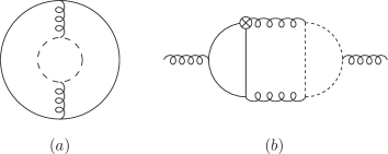
Figure 1: Examples for $3$–loop diagrams $\propto~{}n_{f}$. Solid lines: heavy quarks, dashed lines: light quarks, curly lines: gluons. $\otimes$: operator insertion.

The calculation of the massive tadpole shown in Figure 1, (a), is straightforward. After integrating out the light quark loop, one is left with a $2$–loop massive tadpole, for which the result is known analytically for arbitrary exponents of the propagators. However, as in the $2$–loop case, the calculation is significantly more complicated once the operator insertion is present. Nevertheless, all momentum integrals could be re–written in terms of up to two fourfold sums. These sums differed in their structure from those encountered in the $2$–loop case, making the calculation significantly more complicated. Here, we refer to [10] for more details on how these sums were calculated using the MATHEMATICA–based program Sigma, [24].

Let us now present some of our results. For the $n_{f}^{2}$–term of the $3$–loop anomalous dimension $\gamma_{qg}^{(2)}$ we obtain

$$\gamma_{qg}^{(2)} = n_{f}^{2}T_{f}^{2}C_{A}\Biggl{\{}\frac{32(N^{2}+N+2)}{9N(N+1)(N+2)}\Bigl{[}12S_{2,1}$$ (5)

$$+12S_{-3}+2S_{3}-3S_{2}S_{1}+S_{1}^{3}\Bigr{]}$$

$$-\frac{128(5N^{2}+8N+10)}{9N(N+1)(N+2)}S_{-2}$$

$$-\frac{64P_{1}S_{2}+64P_{2}S_{1}^{2}}{9N(N+1)^{2}(N+2)^{2}}$$

$$+\frac{64P_{3}S_{1}}{27N(N+1)^{3}(N+2)^{3}}$$

$$+\frac{16P_{4}}{27(N-1)N^{4}(N+1)^{4}(N+2)^{4}}\Biggr{\}}$$

$$+n_{f}^{2}T_{f}^{2}C_{F}\Biggl{\{}\frac{32(N^{2}+N+2)}{9N(N+1)(N+2)}\Bigl{[}10S_{3}$$

$$-3S_{1}S_{2}-S_{1}^{3}\Bigr{]}+\frac{32(5N^{2}+3N+2)}{3N^{2}(N+1)(N+2)}S_{2}$$

$$+\frac{32(10N^{3}+13N^{2}+29N+6)}{9N^{2}(N+1)(N+2)}S_{1}^{2}$$

$$-\frac{32P_{5}S_{1}}{27N^{2}(N+1)^{2}(N+2)}$$

$$+\frac{4P_{6}}{27(N-1)N^{5}(N+1)^{5}(N+2)^{4}}\Biggr{\}}~{},$$

with the polynomials

$$P_{1} = 5N^{4}+26N^{3}+47N^{2}+43N+20~{},$$ (6)

$$P_{2} = 5N^{4}+20N^{3}+41N^{2}+49N+20~{},$$ (7)

$$P_{3} = 19N^{6}+124N^{5}+492N^{4}+1153N^{3}$$ (8)

$$+1362N^{2}+712N+152~{},$$

$$P_{4} = 1152+7296N+19904N^{2}$$ (9)

$$+30864N^{3}+25896N^{4}+6800N^{5}$$

$$-10364N^{6}-8899N^{7}+3557N^{8}+8534N^{9}$$

$$+5194N^{10}+1485N^{11}+165N^{12}~{},$$

$$P_{5} = 47N^{4}+145N^{3}+426N^{2}+412N$$ (10)

$$+120~{},$$

$$P_{6} = 99N^{14}+990N^{13}+4925N^{12}$$ (11)

$$+17916N^{11}+46649N^{10}+72446N^{9}$$

$$+32283N^{8}-95592N^{7}-267524N^{6}$$

$$-479472N^{5}-586928N^{4}-455168N^{3}$$

$$-269760N^{2}-122112N-27648~{}.$$

The above and the following expressions are given in terms of harmonic sums, [25, 26], taken at argument $N$. Note that we perform an analytic continuation to complex values of $N$ starting from the even moments. Eq. (5) agrees with the corresponding results in the literature for the case of general values of $N$ and for fixed moments [8, 9, 16]. Our new result is the constant term, which reads

$$a_{Qg}^{(3)} = n_{f}T_{f}^{2}C_{A}\Biggl{\{}\frac{16(N^{2}+N+2)}{27N(N+1)(N+2)}\Bigl{[}-6S_{3,1}$$ (12)

$$+108S_{-2,1,1}-78S_{2,1,1}-90S_{-3,1}+72S_{2,-2}$$

$$-108S_{-2,1}S_{1}+42S_{2,1}S_{1}-6S_{-4}+90S_{-3}S_{1}$$

$$+118S_{3}S_{1}+120S_{4}+18S_{-2}S_{2}+54S_{-2}S_{1}^{2}$$

$$+33S_{2}S_{1}^{2}+15S_{2}^{2}+2S_{1}^{4}+18S_{-2}\zeta_{2}+9S_{2}\zeta_{2}$$

$$+9S_{1}^{2}\zeta_{2}-42S_{1}\zeta_{3}\Bigr{]}-\frac{64Q_{1}S_{2,1}+16Q_{2}S_{2}S_{1}}{27N(N+1)^{2}(N+2)^{2}}$$

$$+\frac{32Q_{3}(6S_{-2,1}-5S_{-3}-6S_{-2}S_{1})}{27N(N+1)^{2}(N+2)^{2}}$$

$$-\frac{16Q_{4}S_{1}^{3}+144Q_{5}S_{1}\zeta_{2}}{81N(N+1)^{2}(N+2)^{2}}$$

$$+\frac{32Q_{6}S_{-2}+8Q_{7}S_{1}^{2}}{81N(N+1)^{3}(N+2)^{3}}$$

$$-\frac{32Q_{8}S_{3}-4032Q_{9}\zeta_{3}}{81(N-1)N^{2}(N+1)^{2}(N+2)^{2}}$$

$$+\frac{Q_{10}S_{2}-9Q_{11}\zeta_{2}}{81(N-1)N^{3}(N+1)^{3}(N+2)^{3}}$$

$$+\frac{N^{3}(N+1)(N+2)Q_{12}S_{1}-Q_{13}}{243(N-1)N^{5}(N+1)^{5}(N+2)^{5}}\Biggr{\}}$$

$$+n_{f}T_{f}^{2}C_{F}\Biggl{\{}\frac{16(N^{2}+N+2)}{27N(N+1)(N+2)}\Bigl{[}144S_{2,1,1}$$

$$-72S_{3,1}-72S_{2,1}S_{1}+48S_{4}-16S_{3}S_{1}-24S_{2}^{2}$$

$$-12S_{2}S_{1}^{2}-2S_{1}^{4}-9S_{1}^{2}\zeta_{2}+42S_{1}\zeta_{3}\Bigr{]}$$

$$+32\frac{10N^{3}+49N^{2}+83N+24}{81N^{2}(N+1)(N+2)}\Bigl{[}3S_{2}S_{1}+S_{1}^{3}\Bigr{]}$$

$$-\frac{128(N^{2}-3N-2)}{3N^{2}(N+1)(N+2)}S_{2,1}$$

$$-\frac{96Q_{14}(N+1)S_{1}^{2}+16Q_{15}S_{1}}{243N^{2}(N+1)^{3}(N+2)}$$

$$+\frac{16(5N^{3}+11N^{2}+28N+12)S_{1}\zeta_{2}}{9N^{2}(N+1)(N+2)}$$

$$-\frac{Q_{16}S_{3}+9Q_{17}\zeta_{3}}{81(N-1)N^{3}(N+1)^{3}(N+2)^{2}}$$

$$+\frac{Q_{18}S_{2}+3Q_{19}\zeta_{2}}{27(N-1)N^{4}(N+1)^{4}(N+2)^{3}}$$

$$+\frac{Q_{20}}{243(N-1)N^{6}(N+1)^{6}(N+2)^{5}}\Biggr{\}}~{}.$$

The terms $Q_{1}\ldots Q_{20}$ are rather lengthy irreducible polynomials in $N$ which will be given in Ref. [22]. Eq. (12) agrees for fixed moments with the results of Ref. [8]. The term $A_{Qg}^{(3)}$ forms the most complex contribution to the $O(n_{f})$ terms of the massive OMEs, along with the term $A_{qg,Q}^{(3)}$. The latter as well as the $O(n_{f})$–terms of $A_{Qq}^{{\sf PS},(3)}$, $A_{qq,Q}^{{\sf PS},(3)}$, $A_{qq,Q}^{{\sf NS},(3)}$ and $\Delta_{T}A_{qq,Q}^{{\sf NS},(3)}$ have been obtained by us as well and will be presented in [22] in detail. Furthermore, the corresponding contributions to the remaining 3-loop anomalous dimensions in the vector– and transversity case are obtained. In this way, an independent recalculation of these quantities given in [9, 15, 16] before, was performed using very different methods.

Finally, it is interesting to consider the small– and large–$N$ limits. We obtain for the $n_{f}$–terms of the renormalized OME $A_{Qg}^{(3)}$

$$\lim_{N\rightarrow 1}(N-1)A_{Qg}^{(3)}=T_{f}^{2}n_{f}\Biggl{\{}\Biggl{(}-\frac{64}{27}C_{A}-\frac{128}{27}C_{F}\Biggr{)}$$

$$\times\ln^{3}\Bigl{(}\frac{m^{2}}{\mu^{2}}\Bigr{)}+\Biggl{(}\frac{416}{27}C_{A}-\frac{832}{27}C_{F}\Biggr{)}\ln^{2}\Bigl{(}\frac{m^{2}}{\mu^{2}}\Bigr{)}$$

$$+\Biggl{(}-\frac{32}{27}C_{A}-\frac{8512}{81}C_{F}\Biggr{)}\ln\Bigl{(}\frac{m^{2}}{\mu^{2}}\Bigr{)}+C_{A}\Bigl{(}\frac{13088}{729}$$

$$+\frac{512}{27}\zeta_{3}\Bigr{)}+C_{F}\Bigl{(}-{\frac{122432}{729}}+{\frac{1024}{27}}\zeta_{3}\Bigr{)}\Biggr{\}}~{},$$ (13)

$$\lim_{N\rightarrow\infty}A_{Qg}^{(3)}=T_{f}^{2}n_{f}\frac{C_{F}-C_{A}}{N}\Biggl{\{}-\frac{20}{27}\hat{\ln}^{4}(N)$$

$$+\Biggl{(}-\frac{32}{9}\ln\Bigl{(}\frac{m^{2}}{\mu^{2}}\Bigr{)}+\frac{320}{81}\Biggr{)}\hat{\ln}^{3}(N)\Biggr{\}}$$

$$+O\Bigl{(}\frac{\hat{\ln}^{2}(N)}{N}\Bigr{)}~{},$$ (14)

$$\hat{\ln}(N)\equiv\ln(N)+\gamma_{E}~{},$$ (15)

with $\gamma_{E}$ being the Euler–Mascheroni constant. The $n_{f}$–contributions at $O(a_{s}^{3})$ to the massive OMEs contain nested harmonic sums up to weight w = 4. This also applies to all individual Feynman diagrams, which we calculated in Feynman–gauge. After reducing the contributing harmonic sums to their common basis using algebraic relations [27] between them, the following harmonic sums contribute

$$S_{1},~{}\quad S_{2},~{}S_{-2},~{}\quad S_{3},~{}S_{-3},$$

$$S_{2,1},~{}S_{-2,1},~{}\quad S_{4},~{}S_{-4},$$

$$S_{3,1},~{}S_{-3,1},~{}S_{-2,2},~{}\quad S_{2,1,1},~{}S_{-2,1,1}~{}.$$ (16)

Note that this set of harmonic sums does not contain the index $\{-1\}$. Due to the structural relations [28, 30], differentiation and argument-duplication, cf. [26], the set (3) can be reduced even further. $S_{1}$ represents the class of all single harmonic sums. Hence only the six basic harmonic sums

$$S_{1}~{},S_{2,1},~{}S_{-2,1}~{},S_{-3,1},~{}S_{2,1,1},~{}S_{-2,1,1}~{}.$$ (17)

are needed to represent the 3-loop results for the $n_{f}$–contributions to the OMEs.

In intermediate steps, we also observed so-called generalized harmonic sums [29, 30]. They obey the following recursive definition [29] :

$$\widetilde{S}_{m_{1},...}(x_{1},...;N)=$$

$$\sum_{i_{1}=2}^{N}\frac{x_{1}^{i_{1}}}{i_{1}^{m_{1}}}\sum_{i_{2}=1}^{i_{1}-1}\frac{x_{2}^{i_{2}}}{i_{2}^{m_{2}}}\widetilde{S}_{m_{3},...}(x_{3},...;i_{2})$$

$$+\widetilde{S}_{m_{1}+m_{2},m_{3},...}(x_{1}\cdot x_{2},x_{3},...;N)~{}.$$ (18)

In the present calculation the values of $x_{i}$ extend to $\{-1/2,1/2,-2,2\}$. These sums occur in ladder like structures, cf. [3, 22, 31] and the next section. They may also emerge, however, if contributions to $3$–loop Feynman diagrams containing a 2-point insertion are separated into various terms in an arbitrary way. The weight of these sums can reach w = 5, although only w = 4 sums should remain in the final results. Examples for these sums are :

$$\widetilde{S}_{1}(1/2;N),~{}~{}\widetilde{S}_{2}(-2;N),~{}~{}\widetilde{S}_{2,1}(-1,2;N),~{}~{}$$

$$\widetilde{S}_{3,1}(-2,-1/2;N),~{}~{}\widetilde{S}_{2,3}(-2,-1/2;N),~{}~{}$$

$$\widetilde{S}_{1,1,1,2}(-1,1/2,2,-1;N),~{}~{}{\rm etc.}$$ (19)

The algebraic and structural relations for these sums are worked out in Ref. [30]. Similar to the case of harmonic sums, corresponding basis representations are obtained. Expressing our results in terms of this common basis, all generalized harmonic sums canceled for each individual diagram. In the beginning, however, it has been unclear, whether this was bound to happen. It is not excluded that these sums contribute in the final results of some of the massive OMEs at 3–loop order.

4 Ladder–type structures

As the next step towards a complete calculation of the $3$–loop OMEs, we consider diagrams deriving from the ladder–type topology shown in Figure 2, cf. [31]. Contrary to the diagram shown in Figure 1(a), it can not trivially be reduced to a $2$–loop diagram.

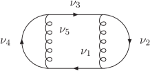
Figure 2: $3$–loop ladder tadpole. $\nu_{i}$ denote exponents of the propagators.

However, one finds that in the scalar case it can be represented in terms of an Appell–function of the first kind, $F_{1}$,

$$F_{1}\Bigl{[}a;b,b^{\prime};c;x_{3},x_{4}\Bigr{]}$$

$$=\sum_{m,n=0}^{\infty}\frac{(a)_{m+n}(b)_{n}(b^{\prime})_{m}}{(1)_{m}(1)_{n}(c)_{m+n}}x_{3}^{n}x_{4}^{m}~{}=\int_{0}^{1}dx_{1}$$

$$\times\int_{0}^{1-x_{1}}dx_{2}\frac{x_{1}^{b-1}x_{2}^{b^{\prime}-1}(1-x_{1}-x_{2})^{c-b-b^{\prime}-1}}{(1-x_{1}x_{3}-x_{2}x_{4})^{a}}~{},$$

(20)

for arbitrary exponents of the propagators. This leads to a double infinite sum ($\nu_{ij}=\nu_{i}+\nu_{j}$, etc.)

$$I_{2}\propto\sum_{{{m}},{{n}}=0}^{\infty}\frac{(-2-\varepsilon/2+\nu_{12})_{m}(-2-\varepsilon/2+\nu_{45})_{n}}{(-4-\varepsilon+\nu_{12345})_{n+m}}$$

$$\cdot\frac{(2+\varepsilon/2)_{m+n}(2+m+\varepsilon/2)_{-\nu_{1}}(2+n+\varepsilon/2)_{-\nu_{5}}}{m!n!},$$

with $(a)_{c}\equiv\Gamma(a+c)/\Gamma(a)$ the Pochhammer symbol. We checked this representation for various integer values of the $\nu_{i}$ using MATAD and found complete agreement. Note that for all diagrams deriving from this topology, the $F_{1}$–structure occurs due to the diagram’s topology and mass distribution, and its form is independent of the operator insertion. As in the previous section and in the $2$–loop case, this allows to obtain a representation in terms of a multiply nested sum, which is regularized and can be expanded in $\varepsilon$, for each diagram belonging to this class. Consider as an example the scalar diagram shown in Figure 3, with all $\nu_{i}=1$.

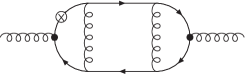
Figure 3: Example $3$–loop ladder diagram.

One obtains the following parameter integral

$$I_{3}=C_{3}\int_{0}^{1}dx_{i}~{}x_{3}^{\frac{\varepsilon}{2}-1}(1-x_{3})^{\frac{\varepsilon}{2}}x_{4}^{\frac{\varepsilon}{2}-1}$$

$$(1-x_{4})^{\frac{\varepsilon}{2}}(x_{5}(1-x_{4})+x_{4}x_{6}(1-x_{1}-x_{2})$$

$$+x_{4}x_{1}x_{7}+x_{4}x_{2}x_{5})^{N-1}x_{1}^{-\frac{\varepsilon}{2}}x_{2}^{-\frac{\varepsilon}{2}}\theta(1-x_{1}-x_{2})$$

$$(1-x_{1}-x_{2})$$

$$\left(1-x_{1}\frac{x_{3}-1}{x_{3}}-x_{2}\frac{x_{4}-1}{x_{4}}\right)^{-2+3\varepsilon/2}~{}.$$ (22)

$C_{3}$ is a trivial pre-factor. The operator insertion contributes as a polynomial linear in each Feynman parameter raised to the power $N$. This term is in a certain sense “convoluted” with a structure deriving from the $F_{1}$ in Eq. (20). The application of the binomial theorem implies additional sums, until the integrand is given in such a way that Eq. (20) can be applied . Thus one obtains:

$$I_{3}=\frac{C_{3}}{(N+1)(N+2)}\sum_{m=0}^{\infty}\sum_{n=0}^{\infty}\sum_{l=2}^{N+2}{N+2\choose l}\sum_{j=2}^{l}$$

$${l\choose j}\Biggl{\{}\sum_{k=1}^{j}{j\choose k}\sum_{r=0}^{l-k}{l-k\choose r}(-1)^{l+j+k+r}$$

$$B\left(k,m+1+\frac{\varepsilon}{2}\right)\frac{\Gamma(k+r+m+n+\frac{\varepsilon}{2})}{\Gamma(m+1)\Gamma(n+1)\Gamma(k+r+\frac{\varepsilon}{2})}$$

$$\frac{B\left(r+l-1,n+1+\frac{\varepsilon}{2}\right)}{(N+3-j)}$$

$$\frac{B\left(k+m-\frac{\varepsilon}{2},r+1+n-\frac{\varepsilon}{2}\right)}{(k+r+1+m+n-\varepsilon)}$$

$$+\sum_{r=0}^{l-j}{l-j\choose r}(-1)^{l+j+r}B\left(r+l-1,n+1+\frac{\varepsilon}{2}\right)$$

$$\frac{\Gamma(j+r+m+n+\frac{\varepsilon}{2})}{\Gamma(m+1)\Gamma(n+1)\Gamma(j+r+\frac{\varepsilon}{2})}B\left(j,m+1+\frac{\varepsilon}{2}\right)$$

$$\frac{B\left(j+m-\frac{\varepsilon}{2},r+1+n-\frac{\varepsilon}{2}\right)}{(j+r+1+m+n-\varepsilon)(N+3-j)}\Biggr{\}}~{}.$$ (23)

Here, $B(a,b)$ is the Euler–Beta function. After expanding in $\varepsilon$, this sum can be reduced by Sigma, cf. [10] and references therein. One obtains

$$I_{3}=\frac{C_{3}}{(N+1)(N+2)(N+3)}\Biggl{\{}\frac{1}{6}{S_{1}^{3}}$$

$$+\frac{N^{2}+12N+16}{2(N+1)(N+2)}{S_{1}^{2}}+\frac{4(2N+3)}{(N+1)^{2}(N+2)}{S_{1}}$$

$$+\frac{8(2N+3)}{(N+1)^{3}(N+2)}+2\Biggl{[}-2^{N+3}+3-(-1)^{N}\Biggr{]}\zeta_{3}$$

$$-(-1)^{N}{S_{-3}}+\Biggl{[}\frac{3N^{2}+40N+56}{2(N+1)(N+2)}-\frac{1}{2}{S_{1}}\Biggr{]}{S_{2}}$$

$$-\frac{3N+17}{3}{S_{3}}-2(-1)^{N}{S_{-2,1}}-(N+3){S_{2,1}}$$

$$+2^{N+4}{S_{1,2}}\left(\frac{1}{2},1;N\right)$$

$$+2^{N+3}{S_{1,1,1}}\left(\frac{1}{2},1,1;N\right)\Biggr{\}}+O(\varepsilon)~{}.$$ (24)

It is interesting to note, that in this case generalized harmonic sums appear in the result for one scalar integral. For the $n_{f}$–terms, this never happened. There, the generalized sums emerged only when splitting up the complete contribution to one diagram into several pieces, without further reference to certain momentum integrals anymore. This could point towards generalized harmonic sums remaining for individual diagrams or even for the complete physical OME. Another interesting point is that the powers $2^{N}$ lead to divergences as $N\rightarrow\infty$ and are therefore expected to cancel in the physical expression. Details on how to calculate this class of ladder–type diagrams and results for the most complicated scalar integrals will be given in [31] .

5 Conclusions

The heavy flavor 3–loop Wilson coefficients are needed in consistent analyses of the DIS World data at NNLO. In case of the structure function $F_{2}(x,Q^{2})$, the asymptotic representation applies for scales $Q^{2}/m^{2}\geq 10$. After a larger number of Mellin moments were computed, now the asymptotic massive Wilson coefficients are calculated for general values of the Mellin variable $N$. Here, we studied both the bubble- and ladder topologies and developed the corresponding computational frame. A first class of contributions has been completed in the case of the quarkonic operator insertions with all contributions to the color factors $T_{F}^{2}n_{f}C_{A,F}$.

References

• [1] See e.g. J. Blümlein, H. Böttcher, A. Guffanti, Nucl. Phys.  B774 (2007) 182; hep-ph/0407089;
S. Alekhin, J. Blümlein, S. Klein, S.-O. Moch, Phys. Rev.  D81 (2010) 014032.
• [2] E. Laenen, et al., Nucl. Phys.  B 392 (1993) 162; S. Riemersma, J. Smith and W. L. van Neerven, Phys. Lett.  B 347 (1995) 143.
• [3] J. A. M. Vermaseren, A. Vogt and S. Moch, Nucl. Phys.  B 724 (2005) 3.
• [4] M. Buza, et al., Nucl. Phys.  B 472 (1996) 611.
• [5] I. Bierenbaum, J. Blümlein and S. Klein, Nucl. Phys.  B 780 (2007) 40; Phys. Lett.  B 648 (2007) 195.
• [6] J. Blümlein, et al. Nucl. Phys.  B 755 (2006) 272.
• [7] M. Buza, et al., Eur. Phys. J.  C 1 (1998) 301.
• [8] I. Bierenbaum, J. Blümlein and S. Klein, Nucl. Phys.  B 820 (2009) 417.
• [9] S. A. Larin, T. van Ritbergen and J. A. M. Vermaseren, Nucl. Phys.  B 427 (1994) 41; S. A. Larin, et al., Nucl. Phys.  B 492 (1997) 338; A. Retey and J. A. M. Vermaseren, Nucl. Phys.  B 604 (2001) 281; J. Blümlein and J. A. M. Vermaseren, Phys. Lett.  B 606 (2005) 130; S. Moch, J. A. M. Vermaseren and A. Vogt, Nucl. Phys.  B 688 (2004) 101; Nucl. Phys.  B 691 (2004) 129.
• [10] J. Ablinger et al. Modern Summation Methods and the Computation of 2- and 3-loop Feynman Diagrams, [arXiv:1006.4797 [math-ph]] and these proceedings.
• [11] I. Bierenbaum, J. Blümlein and S. Klein, Phys. Lett.  B 672 (2009) 401.
• [12] J. Blümlein, S. Klein and B. Tödtli, Phys. Rev.  D 80 (2009) 094010.
• [13] I. Bierenbaum, et al., Nucl. Phys.  B 803 (2008) 1.
• [14] D. J. Broadhurst, et al. Z. Phys.  C 48 (1990) 673; 52 (1991) 111.
• [15] J. A. Gracey, Nucl. Phys. B662, 247 (2003) ; Nucl. Phys. B667, 242 (2003) ; JHEP 10, 040 (2006) ; Phys. Lett. B643, 374 (2006) ;
• [16] J. A. Gracey, Phys. Lett. B 322 (1994) 141 .
• [17] I. Bierenbaum, J. Blümlein and S. Klein, in preparation (2010) .
• [18] P. Nogueira, J. Comput. Phys.  105 (1993) 279.
• [19] T. van Ritbergen, A. N. Schellekens and J. A. M. Vermaseren, Int. J. Mod. Phys.  A 14 (1999) 41.
• [20] M. Steinhauser, Comput. Phys. Commun.  134 (2001) 335 and ${\sf MATAD~{}3.0}$.
• [21] J. A. M. Vermaseren, New features of FORM, [math-ph/0010025].
• [22] J. Ablinger, J. Blümlein, S. Klein, C. Schneider and F. Wißbrock, in preparation (2010) .
• [23] F. Wißbrock, Diploma Thesis, Freie Universität Berlin (2010) .
• [24] C. Schneider, J. Symbolic Comput. 43 (2008) 611, [arXiv:0808.2543v1]; Ann. Comb. 9 (2005) 75; J. Differ. Equations Appl. 11 (2005) 799; Ann. Comb. (2009) to appear, [arXiv:0808.2596]; Proceedings of the Conference on Motives, Quantum Field Theory, and Pseudodifferential Operators, To appear in the Mathematics Clay Proceedings, 2010; Sém. Lothar. Combin. 56 (2007) 1, Article B56b, Habilitationsschrift JKU Linz (2007) and references therein.
• [25] J. Vermaseren, Int. J. Mod. Phys. A14 (1999) 2037 .
• [26] J. Blümlein and S. Kurth, Phys. Rev. D 60 (1999) 014018 .
• [27] J. Blümlein, Comput. Phys. Commun. 159 (2004) 19 .
• [28] J. Blümlein, Comput. Phys. Commun. 180 (2009) 2218; arXiv:arXiv:0901.0837 .
• [29] S. Moch, P. Uwer, S. Weinzierl, Stefan, J. Math. Phys. 43 (2002) 3363-3386 .
• [30] J. Ablinger, J. Blümlein, C. Schneider, in preparation (2010) .
• [31] J. Blümlein, A. Hasselhuhn, S. Klein, C. Schneider, in preparation (2010) .