Event-by-event hydrodynamics and elliptic flow from fluctuating initial state

Abstract

We develop a framework for event-by-event ideal hydrodynamics to study the differential elliptic flow which is measured at different centralities in Au+Au collisions at Relativistic Heavy Ion Collider (RHIC). Fluctuating initial energy density profiles, which here are the event-by-event analogues of the eWN profiles, are created using a Monte Carlo Glauber model. Using the same event plane method for obtaining $v_{2}$ as in the data analysis, we can reproduce both the measured centrality dependence and the $p_{T}$ shape of charged-particle elliptic flow up to $p_{T}\sim 2$ GeV. We also consider the relation of elliptic flow to the initial state eccentricity using different reference planes, and discuss the correlation between the physical event plane and the initial participant plane. Our results demonstrate that event-by-event hydrodynamics with initial state fluctuations must be accounted for before a meaningful lower limit for viscosity can be obtained from elliptic flow data.

I Introduction

Azimuthal anisotropy of final state particles produced in ultrarelativistic heavy ion collisions can be used to measure the collective behavior of the dense particle system formed in such collisions Ollitrault:1992bk . The strong azimuthal anisotropy, which has been observed in the transverse momentum spectra of hadrons in Au+Au collisions at the Relativistic Heavy Ion Collider (RHIC) of the Brookhaven National Laboratory, is also a signature of the formation of strongly interacting partonic matter, the Quark-Gluon Plasma (QGP).

Ideal hydrodynamics has been successful in predicting and explaining the measured elliptic flow in Au+Au collisions at RHIC Hirano:2001eu ; Hirano:2002ds ; Huovinen:2001cy ; Huovinen:2005gy ; Huovinen:2007xh ; Kolb:2000sd ; Kolb:2001qz ; Nonaka:2006yn ; Schenke:2010nt ; Teaney:2001av ; Teaney:2000cw ; Niemi:2008ta . Currently, a lot of effort is devoted for developing a description of the QCD-matter evolution in terms of dissipative hydrodynamics. The recent results show that even a small viscosity can considerably decrease the elliptic flow Romatschke:2007mq ; Luzum:2008cw ; Song:2007fn ; Song:2007ux ; Song:2009rh ; Dusling:2007gi .

However, all these ideal and viscous hydrodynamic studies tend to underestimate the elliptic flow in most central collisions. Generally, the explanation for the deficit has been thought to be the initial state density fluctuations which have not been accounted for. In addition to taking into account the density fluctuations themselves, special care should be taken in computing the elliptic flow with respect to the same reference plane as in the data analysis.

The initial state fluctuations can be implemented e.g. via a Monte Carlo Glauber (MCG) model which makes possible to study the fluctuations of the initial matter eccentricity. Geometric fluctuations in the positions of nucleons have been shown to increase the initial eccentricity, which is then suggested to translate into elliptic flow of final state particles Alver:2008zza . Furthermore, the reference plane plays a crucial role: the eccentricity is larger if one calculates it using the participant plane (determined by the transverse positions of the participant nucleons and the beam axis) instead of the reaction plane (determined by the impact parameter and the beam axis).

Recently, in Ref. Hirano:2009ah , hydrodynamical calculations were performed using averaged initial density profiles which were obtained from MCG calculations. Before averaging over the profiles, the transverse coordinate axes were rotated in each event so that the participant planes were on top of each other. In this manner it is possible to get an averaged initial profile that takes into account the eccentricity fluctuations in the initial state. For Au+Au collisions at RHIC, however, the effects of such plane rotations on the integrated $v_{2}$ were small.

While the above studies are steps to the right direction, it is obvious that without doing event-by-event hydrodynamic simulations, it is impossible to know how closely the computational participant plane corresponds to the physical event plane which is determined from the observed final state hadron momenta.

So far, genuine event-by-event models where hydrodynamics is run event by event using fluctuating initial density profiles, have been presented in Refs. Hama:2004rr ; Andrade:2006yh ; Andrade:2008xh ; Werner:2010aa ; Petersen:2009vx ; Petersen:2010md . Interestingly, a similar two-particle correlation ridge as observed in the experiments :2009qa , is seen to form into the rapidity–azimuth-angle –plane both in NeXSpherio Andrade:2008xh and more recently in Ref. Werner:2010aa . This suggests that the puzzling ridge may well be another consequence of the fluctuations in the initial state.

Also higher flow coefficients have been measured Adams:2003zg ; Abelev:2007qg ; :2010ux and recent studies Gombeaud:2009ye show that the initial state density fluctuations may play an important role in understanding the centrality dependence of the ratio $v_{4}/(v_{2})^{2}$. Triangular flow arising from event-by-event fluctuations Alver:2010gr is also one of the things that should be studied further with event-by-event hydrodynamics.

In this paper, we introduce an event-by-event ideal hydrodynamics framework to study the following $v_{2}$-related problems: With ideal hydrodynamics using averaged initial states, (i) there is a $v_{2}$ deficit in central collisions, as discussed above; (ii) the shape and centrality dependence of $v_{2}(p_{T})$ are unsatisfactory in that the $p_{T}$ slopes of $v_{2}$ easily become too steep and elliptic flow increases too much towards noncentral collisions; (iii) elliptic flow is computed relative to the initial reaction plane or in the best case to the participant plane Hirano:2009ah but not relative to the event plane, which is commonly used in the experiments; (iv) one does not know how closely the event plane and the initial participant plane correspond to each other. A concrete illustration of the problems (i)–(ii) can be found in Fig. 7.5. of Ref. Niemi:2008zz , and also in Fig. 5 of our previous elliptic flow study Niemi:2008ta .

We will show how event-by-event ideal hydrodynamics, initiated with a fluctuating initial density profile obtained from a MC Glauber model, and especially the determination of $v_{2}$ with respect to the event plane, conveniently solves the problem of the $v_{2}$ deficit in the most central Au+Au collisions at RHIC. Simultaneously, we can significantly improve the agreement with the data for $v_{2}$ at all centrality classes up to 30-40% most central collisions in the typical applicability region of hydrodynamics, $p_{T}<2$ GeV. This in turn has the very important implication that viscous effects can in fact be allowed to be smaller than previously thought. Finally, we also show the correspondence between the event and participant planes and study the relation between the elliptic flow and initial eccentricity using different reference planes.

The rest of the paper is constructed as follows: First, in Sec. II we introduce our framework for event-by-event hydrodynamics. Details discussed there are our MCG model, computation of the fluctuating initial energy density profiles, MC modeling of thermal spectra of final state hadrons, and MC modeling of the resonance decays. We also try to discuss the points where our modeling could be improved. Section III is devoted for defining the event plane and elliptic flow. Also eccentricity issues are discussed there. Our results are presented in Sec. IV and conclusions are given in Sec. V.

II Event-by-event hydrodynamics framework

II.1 MC Glauber model and centrality classes

We use here a MCG model to define the centrality classes and to form initial states with fluctuating density profiles. First, we distribute the nucleons in the colliding nuclei randomly using the standard, spherically symmetric, two-parameter Woods-Saxon (WS) nuclear density profile as the probability distribution. Our WS parameters for the gold nucleus are $R_{A}\approx 6.37\rm{~{}fm}$ for the radius and $d=0.54\rm{~{}fm}$ for the surface thickness. In the transverse $(x,y)$ plane the two nuclei are separated by an impact parameter $b$ between the centers of mass of the nuclei, which is determined by sampling the distribution $dN/db\propto b$ in the region $0\leq b\leq b_{\text{max}}=20\rm{~{}fm}>2r_{0}$. The longitudinal $z$ coordinate is taken into account when sampling the initial nucleon positions but in what follows it does not play any role.

Nucleons $i$ and $j$ from different nuclei are then assumed to collide if their transverse distance is small enough,

$$(x_{i}-x_{j})^{2}+(y_{i}-y_{j})^{2}\leq\frac{\sigma_{NN}}{\pi},$$ (1)

where $\sigma_{NN}$ is the inelastic nucleon-nucleon cross section. We apply here $\sigma_{NN}=42\rm{~{}mb}$ for Au+Au collisions at $\sqrt{s_{NN}}=200\rm{~{}GeV}$.

We note that our simple MCG model fails to reproduce the correlations between the nucleons, since we use the WS distribution for determining the nucleon positions independently from each other. In Broniowski:2010jd it was observed that a realistic model, which accounts for nucleon correlations Alvioli:2009ab , can be well approximated using an exclusion radius which prevents nucleon overlap. Using such radius, or giving a finite size for the nucleons Hirano:2009ah , causes deviations from the WS distribution which should then be compensated by tuning of the parameters in the initially sampled WS distribution.

To keep our modeling as transparent as possible we, however, choose not to apply an exclusion radius or a nucleon size in our MCG model since according to Ref. Hirano:2009ah only a 10% uncertainty in the initial eccentricity can be expected, which is a much smaller effect than e.g. the overall uncertainties related to the choice of the initial density profiles.

Next, we define the centrality classes using the number of participant nucleons, $N_{\text{part}}$, for simplicity. We have plotted the distribution of events as a function of $N_{\text{part}}$ in Fig. 1. As indicated there, we slice our total event distribution in $N_{\text{part}}$ so that each $N_{\text{part}}$ interval corresponds to a centrality class which contains a certain percent of total events. The impact parameter may thus freely fluctuate within each centrality class.

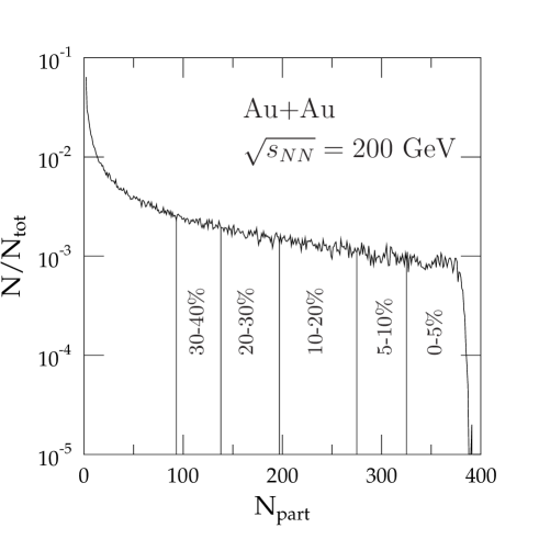
Figure 1: Our definition of centrality classes for Au+Au collisions at $\sqrt{s_{NN}}=200\rm{~{}GeV}$. Distribution of the number of participants is calculated from a Monte Carlo Glauber model without a nucleon exclusion radius.

II.2 Initial density profiles

In order to utilize the MCG-given initial state to start hydrodynamics, we must next somehow transform the positions of the wounded nucleons or binary collisions into energy density or entropy density. These would be the fluctuating event-by-event MCG analogues of the conventional eWN, eBC and sWN, sBC Kolb:2001qz average initial densities. For simplicity, we consider here just the eWN-type of profile and leave the profile fine tuning for future work. The energy density is now distributed in the $(x,y)$ plane around the wounded nucleons using a 2D Gaussian as a smearing function,

$$\epsilon(x,y)=\frac{K}{2\pi\sigma^{2}}\sum_{i=1}^{N_{\text{part}}}\exp\Big{(}-\frac{(x-x_{i})^{2}+(y-y_{i})^{2}}{2\sigma^{2}}\Big{)},$$ (2)

where $K$ is a fixed overall normalization constant and $\sigma$ is a free smearing parameter controlling the width of our Gaussian. In each event, the impact parameter defines the direction of the $x$ axis and the origin of the $(x,y)$ plane is determined so that the energy-density weighted coordinate averages become $\langle x\rangle=\langle y\rangle=0\rm{~{}fm}$.

For the hydrodynamical description to be meaningful, the initial state should not have too sharp density peaks. In our MCG model we have given an effective interaction radius $\sqrt{\sigma_{NN}/\pi}/2\approx 0.6\rm{~{}fm}$ for the colliding nucleons, which sets a natural order of magnitude for $\sigma$. To probe the sensitivity of our results to the initial state smearing, we will consider two values, $\sigma=0.4\rm{~{}fm}$ and 0.8 fm. With the current setup, we cannot reduce $\sigma$ further, as this would require a smaller step size in our hydrodynamical code, and consequently much more CPU time. One should then also develop a way to handle multiple separate freeze-out surfaces, see the discussion in Sec. II.3. These developments we leave as future improvements.

The reason to choose the energy density to be smeared rather than the entropy density, is mostly technical and due to the fact that our focus here is on understanding the transverse flow phenomena. Since we now avoid using the Equation of state in forming the initial energy density profiles in each event, we have a more direct control on the input energy density (pressure) gradients that drive the evolution of the transverse flow and its asymmetries. In our case, the total energy per rapidity unit in each event, $\int dxdy\,\epsilon(x,y)$, thus remains independent of $\sigma$, while the total entropy per rapidity unit and thereby also the final state multiplicity depend on $\sigma$.

For Au+Au collisions at $\sqrt{s_{NN}}=200\rm{~{}GeV}$, we use the value $K=37.8\rm{~{}GeV}/\rm{~{}fm}$. With this, we reproduce the initial total entropy of Ref. Niemi:2008ta when averaging over many initial states in central ($b=0$) collisions when $\sigma=0.4\rm{~{}fm}$. Motivated by the EKRT minijet (final state) saturation model Eskola:1999fc and Ref. Niemi:2008ta , we fix the initial time to $\tau_{0}=0.17\rm{~{}fm}$ for all events.

II.3 Hydrodynamics, freeze out and resonance decays

For obtaining the ideal-fluid hydrodynamic evolution of the system, we solve the standard equations

$$\partial_{\mu}T^{\mu\nu}=0$$ (3)

together with an Equation of State (EoS) which relates pressure with the energy density and net-baryon number density, $P=P(\epsilon,n_{B})$. As we are interested in particle production at mid-rapidity, we assume the net-baryon density to be negligible. Since the rapidity distributions of hadrons are approximately flat at mid-rapidities we can safely simplify our hydrodynamical equations by assuming longitudinal boost-invariance. We solve this (2+1)-dimensional numerical problem using the SHASTA algorithm Boris ; Zalesak which is also able to handle shock waves.

As the Equation of State (EoS), we choose the EoS from Laine and Schröder Laine:2006cp . At high temperatures this EoS has been matched with the lattice-QCD data and at low temperatures with a hadron resonance gas containing particles of mass $m<2\rm{~{}GeV}$. This EoS has a ”cross-over” transition from the QGP to the hadron gas.

Thermal spectra for hadrons are calculated using the conventional Cooper-Frye method Cooper , where particle emission from a constant-temperature surface $\sigma$ is calculated according to

$$\frac{dN}{d^{2}p_{T}dy}=\int_{\sigma}f(x,p)p^{\mu}d\sigma_{\mu},$$ (4)

where $f(x,p)$ is the particle number-distribution function in momentum at a certain space-time location. The freeze-out temperature $T_{\text{dec}}=160$ MeV is fixed so that we reproduce the measured $p_{T}$ spectrum of pions Adler:2003cb when averaged initial states are considered.

Our surface finding algorithm operates in the $(r,\tau)$-plane for all spatial azimuthal angles. Currently, we can find only surfaces which go through $r=0$. Due to the initial state fluctuations there might simultaneously exist also other, disconnected, freeze-out surfaces which our algorithm does not recognize. We have checked that for the centrality classes and smearing parameters $\sigma$ considered here, only a a few percent of the events actually contain such a surface. In any case, since these additional surfaces typically originate from a few-nucleon collisions, they contribute negligibly to particle production in not too peripheral Au+Au collisions. Making $\sigma$ smaller can also increase the number of disconnected freeze-out surfaces. To ensure the applicability of our framework, we prefer not to consider centrality classes more peripheral than 30–40% or $\sigma<0.4\rm{~{}fm}$ in the present study.

For the flow analysis, we need individual final state particles. In generating these using the computed thermal spectrum as the probability distribution, we assume the total number of thermal particles in a rapidity unit to be fixed individually in each event. The transverse momentum $(p_{x},p_{y})$ for each particle is thus sampled from the distribution $dN/d^{2}p_{T}dy$ calculated in Eq. (4). Due to the assumed boost-symmetry, we are not equipped to consider rapidity distributions, thus $y$ is sampled from a flat distribution in the interval $|y|\leq 0.5$.

Note that above we have neglected the fluctuations in the number of emitted thermal particles. In principle one could derive these fluctuations separately from the thermal distributions for each freeze-out surface element. However, it is not so clear how to treat the space-like parts of the surface in this case. Since in the collisions considered here there are of the order of 1000 particles per unit rapidity, these fluctuations can in any case be expected to be negligible in comparison with the initial state fluctuations.

Once we have generated all the thermal hadrons, we still need take into account the strong and electromagnetic decays. We let the thermal resonances decay one by one using PYTHIA 6.4 Sjostrand:2006za . Some decay products can fall outside our rapidity interval $|y|<0.5$. On the other hand, there would also be decay products arriving from $|y|>0.5$ which we do not consider here. We have checked that instead of increasing the width of our thermal particle rapidity window, to speed up the analysis, we can simply count all decay products into our rapidity acceptance regardless of their actual rapidity.

II.4 Event statistics

Our main goal is to compare the event-by-event hydrodynamic results with the ones obtained by more conventional non-fluctuating hydrodynamics initiated with averaged initial states.

For event-by event hydrodynamics, we make 500 hydro runs in each centrality class. This amount of hydro runs seems enough for the hadron spectra and elliptic flow analysis. To increase statistics we make 20 final state events from every hydro run, thus we have 10 000 events in total. To check that using each hydro run 20 times is sensible, we have checked that doing 250 hydro runs and 40 events from each leads to the same flow results.

To create an averaged initial state, we sum together 20 000 initial states generated by our MCG model. Such large number of events is required since fluctuations near the edges of the system easily affect the final value of elliptic flow if the density profile is otherwise smooth. We then do one hydro run with the averaged initial state for each centrality class. To make a fare comparison with the event-by-event hydro results, we do the resonance decays and analysis using the same code for the averaged initial state case as for the event-by-event hydro case, making 10 000 final state events from this one hydro run.

III Elliptic flow analysis

III.1 Elliptic flow and event plane

The transverse momentum spectra of hadrons can be written as a Fourier series,

$$\frac{dN}{d^{2}p_{T}dy}=\frac{1}{\pi}\frac{dN}{dp_{T}^{2}dy}\Big{(}1+2\sum_{n=1}^{\infty}v_{n}\cos(n\phi)\Big{)},$$ (5)

where $\phi$ is the hadron momentum’s azimuthal angle with respect to the reaction plane defined by the impact parameter. The flow coefficients $v_{n}$ can then be computed from

$$v_{n}(p_{T})=\frac{\int d\phi\cos(n\phi)\frac{dN(b)}{dp_{T}^{2}d\phi dy}}{\int d\phi\frac{dN(b)}{dp_{T}^{2}d\phi dy}}.$$ (6)

When we have fluctuations in the initial state, calculation of $v_{n}$ is not so straightforward. In the hydrodynamic runs, where we always know the direction of our impact parameter, we can calculate the elliptic flow with respect to the reaction plane. If we want to compare with experiments, we should use the same analysis methods and definitions as in the data analysis. In this work we use the event plane method Poskanzer:1998yz ; Ollitrault:1997di which is a common way to calculate $v_{2}$. Since it is not (yet) typically used in hydrodynamical calculations, let us briefly recapitulate the main points (see Ref. Poskanzer:1998yz for details).

We first define an event flow vector $\bm{Q_{n}}$ for the $n$th harmonic. The event flow vector in the transverse plane is

$$\bm{Q_{n}}=\sum_{i}(p_{Ti}\cos(n\phi_{i}),p_{Ti}\sin(n\phi_{i})),$$ (7)

where we sum over every particle in the event and where $\phi$ is measured from the $x$ axis which is here fixed by the impact parameter. The event plane angle $\psi_{n}$ for each event is then defined to be

$$\psi_{n}=\frac{\arctan(Q_{n,y}/Q_{n,x})}{n},$$ (8)

with arctan placed into the correct quadrant. The ”observed” $v_{n}$ is calculated with respect to the event planes obtained above,

$$v_{n}\{\text{obs}\}=\langle\langle\cos(n(\phi_{i}-\psi_{n}))\rangle\rangle_{\text{events}},$$ (9)

where the inner angle brackets denote an average over all particles $i$ in one event and the outer ones an average over all events. In order to remove autocorrelations, the particle $i$ is excluded from the determination of the event flow vector when correlating it with the event plane.

Since in our finite rapidity interval we have only a finite number of particles available for the event plane determination, the obtained event plane fluctuates from the ”true” event plane. (In our event-by-event hydrodynamics, the true event plane in each event would correspond to the average event plane obtained by generating infinitely many final states from one hydro run.) The obtained $v_{n}\{\text{obs}\}$ is corrected using the event plane resolution for the harmonic $n$

$$\mathcal{R}_{n}=\langle\cos(n(\psi_{n}-\psi_{n}^{\text{true}}))\rangle,$$ (10)

where $\psi_{n}^{\text{true}}$ defines the true event plane and the angle brackets stand for an average over a large sample of events. Because experimentally it is not possible to find the true event plane, the event plane resolution must be estimated.

In the two-subevents method, which also we will use, each event is randomly divided into two equal subevents $A$ and $B$. The event plane resolution for each of these subevents is then Poskanzer:1998yz

$$\mathcal{R}_{n}^{\text{sub}}=\sqrt{\langle\cos(n(\psi_{n}^{A}-\psi_{n}^{B}))\rangle}.$$ (11)

If the fluctuations from the true event plane are Gaussian, one can analytically obtain the following result Poskanzer:1998yz

$$\mathcal{R}_{n}=\frac{\sqrt{\pi}}{2\sqrt{2}}\chi_{n}\exp(-\chi_{n}^{2}/4)\Big{[}I_{0}(\chi_{n}^{2}/4)+I_{1}(\chi_{n}^{2}/4)\Big{]},$$ (12)

where $I_{0}$ and $I_{1}$ are modified Bessel functions and $\chi_{n}\sim\sqrt{N}$, with $N$ referring to the number of particles. Since we can calculate $\mathcal{R}_{n}^{\text{sub}}$ from the subevents, we can numerically solve $\chi_{n}^{\text{sub}}$ from Eq. (12). Because the number of particles in the subevents is half of those in the full events, $\chi_{n}^{\text{full}}=\sqrt{2}\chi_{n}^{\text{sub}}$, and we can calculate the resolution $\mathcal{R}_{n}^{\text{full}}$ for the full events. Finally, the flow coefficients are obtained as

$$v_{n}=\frac{v_{n}\{\text{obs}\}}{\mathcal{R}_{n}^{\text{full}}}.$$ (13)

The elliptic flow results computed with this method are denoted here as $v_{2}\{\text{EP}\}$. We also compute the elliptic flow from Eq. (9) with respect to the reaction plane using both fluctuating and averaged initial states. In the reaction plane case we have no corrections coming from statistical fluctuations. These results are denoted as $v_{2}\{\text{RP}\}$ in what follows.

III.2 Initial eccentricity and participant plane

The reaction plane eccentricity of the hydrodynamical initial state can be defined as (see e.g. Ref. Alver:2008zza )

$$\epsilon_{\text{RP}}=\frac{\sigma_{y}^{2}-\sigma_{x}^{2}}{\sigma_{y}^{2}+\sigma_{x}^{2}}$$ (14)

where

$$\begin{split}\sigma_{y}^{2}&=\langle y^{2}\rangle-\langle y\rangle^{2}\\ \sigma_{x}^{2}&=\langle x^{2}\rangle-\langle x\rangle^{2},\\ \end{split}$$ (15)

where the averaging is done over the energy density profile of Eq. (2).

Since the positions of wounded nucleons, however, fluctuate from one event to another, tilting the transverse coordinate axes suitably we can actually get a larger eccentricity than $\epsilon_{\text{RP}}$ above. Thus it is not so clear what the most correct reference plane should be.

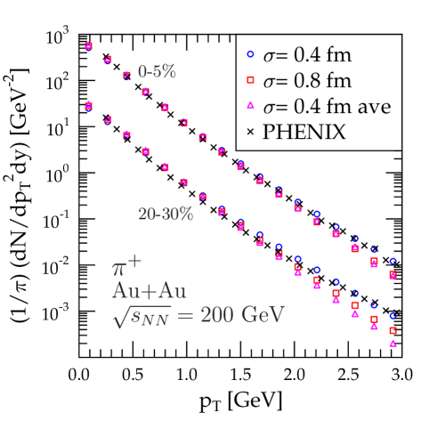
Figure 2: (Color online) Transverse momentum spectra of positive pions for Au+Au collisions at $\sqrt{s_{NN}}=200\rm{~{}GeV}$ calculated with averaged and fluctuating initial states varying the width of Gaussian smearing. Data are from the PHENIX collaboration Adler:2003cb .

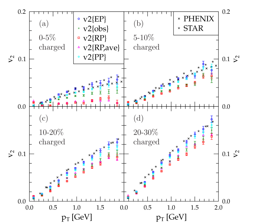
Figure 3: (Color online) Elliptic flow of charged particles as a function of $p_{T}$ at different centralities for Au+Au collisions at $\sqrt{s_{NN}}=200\rm{~{}GeV}$. Hydrodynamical calculations with fluctuating and averaged initial states are shown for $\sigma=0.4\rm{~{}fm}$. Data are from the PHENIX Afanasiev:2009wq ; :2010ux and STAR Adams:2004bi collaborations. The statistical errors in the experimental data are smaller than the symbol size.

The reference plane that maximizes the initial eccentricity can be expected to correlate better with the event plane than the reaction plane. For this purpose, one may define the participant eccentricity Alver:2008zza

$$\epsilon_{\text{PP}}=\frac{\sqrt{(\sigma_{y}^{2}-\sigma_{x}^{2})^{2}+4\sigma_{xy}^{2}}}{\sigma_{y}^{2}+\sigma_{x}^{2}},$$ (16)

where $\sigma_{xy}=\langle xy\rangle-\langle x\rangle\langle y\rangle$. In this case the reference plane is the participant plane which is defined by the $z$ axis (beam direction) and the $x$ axis which is first rotated around the $z$ axis by the angle

$$\psi_{\text{PP}}=\arctan\frac{-2\sigma_{xy}}{\sigma_{y}^{2}-\sigma_{x}^{2}+\sqrt{(\sigma_{y}^{2}-\sigma_{x}^{2})^{2}+4\sigma_{xy}^{2}}}.$$ (17)

In what follows, we will compute the elliptic flow also with respect to the participant plane,

$$v_{2}\{\text{PP}\}=\langle\langle\cos(2(\phi_{i}-\psi_{\text{PP}}))\rangle\rangle_{\text{events}}$$ (18)

and consider the relation of elliptic flow to the initial eccentricity using both the reaction plane and the participant plane as the reference.

IV Results

Below, we present the results for pion spectra, elliptic flow, eccentricities and the correlation of the event and participant planes. The genuine event-by-event calculations using smearings $\sigma=0.4$ and 0.8 fm, are compared with the results obtained using an averaged initial state.

In Fig. 2 we show the $p_{T}$ spectra of positive pions from these three different hydro calculations and from the PHENIX collaboration Adler:2003cb . As explained in Sec. II.2, our multiplicity depends on the Gaussian smearing width $\sigma$, hence the (small) difference between the points with $\sigma=0.4\rm{~{}fm}$ and $\sigma=0.8\rm{~{}fm}$ at low $p_{T}$.

We can also see that at higher $p_{T}$ we get more particles with the fluctuating initial states than with the averaged initial state case. This follows from the fact that in the fluctuating initial states there are larger pressure gradients present. For the same reason, the high-$p_{T}$ spectra are quite sensitive to the value of $\sigma$: with a larger $\sigma$, the pressure gradients are smaller and the $p_{T}$ spectra steeper. This is in fact an interesting observation, suggesting that with fluctuating initial states the applicability region of (event-by-event) hydrodynamics may extend to higher $p_{T}$ than previously (see e.g. Refs. Eskola:2002wx ; Eskola:2005ue ) thought. In any case, the obtained $p_{T}$ spectra agree with the data sufficiently well, so that we can meaningfully next study the elliptic flow.

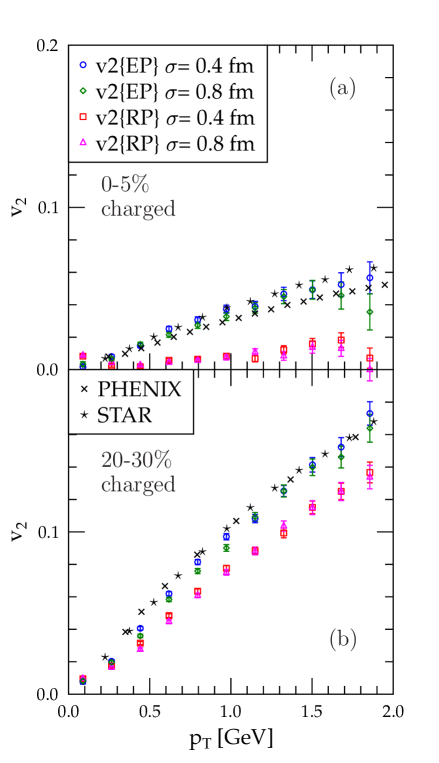
Figure 4: (Color online) Elliptic flow of charged particles as a function of $p_{T}$ at different centralities with two different values for Gaussian smearing parameter $\sigma$.

In Fig. 3 we plot the elliptic flow of charged particles as a function of $p_{T}$ at different centralities. We show the event-by-event results for $v_{2}\{\text{EP}\}$, $v_{2}\{\text{RP}\}$ and $v_{2}\{\text{PP}\}$, as well as $v_{2}\{\text{RP,ave}\}$ which is obtained from averaged initial states.

First, we observe, that $v_{2}\{\text{RP}\}$ and $v_{2}\{\text{RP,ave}\}$ are quite close to each other (although in the panel (c) some statistical fluctuations seem to be still present), and especially that in central collisions there is a significant deficit of $v_{2}$ relative to the data. Second, we see that our $v_{2}\{\text{EP}\}$ agrees very well (within the estimated errors) with the data up to $p_{T}\sim 2$ GeV in all centrality classes. Notice also the difference between the uncorrected $v_{2}\{\text{obs}\}$ and the corrected, final, $v_{2}\{\text{EP}\}$; especially for central collisions, the corrections $\mathcal{R}_{2}$ are quite large. Thus, fluctuations alone are not sufficient in explaining the $v_{2}$ data but that – in addition to taking into account the fluctuations – the computed $v_{2}$ must be defined in the same way as in the experimental analysis.

Third, we notice that the relative increase from $v_{2}\{\text{RP}\}$ to $v_{2}\{\text{EP}\}$ decreases from central to peripheral collisions: $v_{2}\{\text{EP}\}/v_{2}\{\text{RP}\}={\cal O}(10)$ in panel (a) and ${\cal O}(1.2)$ in panel (d). Fourth, contrary to our original expectation, $v_{2}\{\text{RP,ave}\}$ for semi-peripheral collisions is actually below (and not above) the data at $p_{T}\sim 1.5$ GeV. This is due to the fact that with our MCG model and smearing, the actual energy density profiles become flatter and less eccentric than the conventional eWN profiles obtained from an optical Glauber model. As a result, we get a smaller $v_{2}\{\text{RP}\}$ than e.g. in Ref. Niemi:2008ta , and thus also in the 20-30% centrality class there is room for an increase from $v_{2}\{\text{RP}\}$ to $v_{2}\{\text{EP}\}$. From these observations we can conclude that we have answered the questions (i)–(iii) presented in Sec. I.

Fourth, Fig. 3 indicates that $v_{2}\{\text{PP}\}$ is very close to $v_{2}\{\text{EP}\}$ in all centrality classes. This result suggests that the participant plane indeed is quite a good approximation for the event plane.

In Fig. 4 we show the effects of varying our Gaussian smearing parameter $\sigma$. We see that our elliptic flow results are quite insensitive to $\sigma$: Doubling the value of $\sigma$ causes only of the order of 10% changes in our $v_{2}(p_{T})$. We remind, however, that our $p_{T}$-spectra and multiplicity of pions were not as stable against $\sigma$ but we expect that doing more proper fitting to the pion spectra by fine-tuning $T_{\text{dec}}$ and the initial overall normalization constant $K$, would not affect our $v_{2}$ results significantly.

In Fig. 5 we plot the integrated elliptic flow for the four different cases considered above and the data from the PHOBOS collaboration Alver:2006wh . As expected on the basis of Figs. 3 and 2, our results $v_{2}\{\text{EP}\}$ and $v_{2}\{\text{PP}\}$ now agree with the data very well, while the $v_{2}\{\text{RP}\}$ results fall significantly below the data.

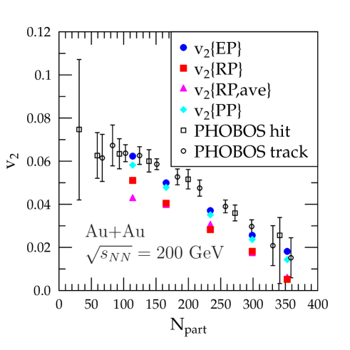
Figure 5: (Color online) Integrated elliptic flow for Au+Au collisions at $\sqrt{s_{NN}}=200\rm{~{}GeV}$ calculated with fluctuating and averaged initial states are shown for $\sigma=0.4\rm{~{}fm}$. Data from the PHOBOS collaboration Alver:2006wh are shown with statistical and systematic errors added in quadrature.

Next, Fig. 6 shows the computational quantity $v_{2}/\epsilon$ which is often discussed. In the PHOBOS result Alver:2006wh , $v_{2}$ is determined relative to the event plane while the initial state eccentricity is computed relative to the participant plane. We reproduce the PHOBOS $v_{2}/\epsilon$ if we do the same, i.e. use $\epsilon_{\text{PP}}$ from Eq. (16). Interestingly, if we replace both the elliptic flow and the eccentricity by their reaction plane analogues, we can still get a scaling law that agrees with our $v_{2}\{\text{EP}\}/\epsilon_{\text{PP}}$ and with the data. This figure illustrates again the importance of the consistency in the reference plane definition.

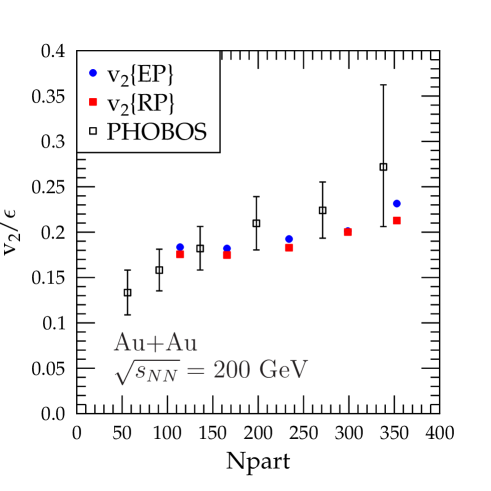
Figure 6: (Color online) Integrated elliptic flow of charged particles for Au+Au collisions at $\sqrt{s_{NN}}=200\rm{~{}GeV}$ divided by initial eccentricity. Theoretical calculations correspond to fluctuating initial states with $\sigma=0.4\rm{~{}fm}$. Data from the PHOBOS collaboration Alver:2006wh are shown with statistical and systematic errors added in quadrature.

Finally, we answer the question (iv) presented in Sec. I. Figure 7 shows the correlation between the event plane and the participant plane as well as the correlation between the event plane and the reaction plane. We plot the distribution of events as a function of the angle differences $\psi_{2}-\psi_{\text{PP}}$ and $\psi_{2}-\psi_{\text{RP}}$. For this figure, we have used each hydro run only once. We notice that in central collisions, the planes are more weakly correlated than in semi-peripheral collisions where clearer peaks around $\psi_{2}=\psi_{\text{PP}},\psi_{\text{RP}}$ arise. As expected based on Fig. 3, the participant plane is indeed found to be quite a good approximation for the event plane, in all centrality classes. However, fluctuations of the event plane around the ”true” event plane are much larger in central collisions and thus the correlation between the event plane and the participant plane in Fig. 7 looks weaker for central collisions than for the more peripheral ones.

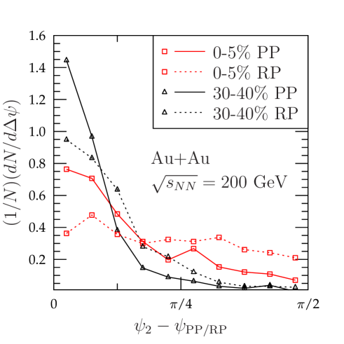
Figure 7: (Color online) Correlation of the event plane with the participant plane, and with the reaction plane at different centralities and with $\sigma=0.4\rm{~{}fm}$. The lines are to guide the eye.

V Conclusions

The main result of this paper is that using event-by-event ideal hydrodynamics with MCG-generated fluctuating initial density profiles we can simultaneously reproduce the measured centrality dependence and the $p_{T}$ shape of charged-particle elliptic flow up to $p_{T}\sim 2$ GeV. Also the measured pion spectra are quite well reproduced, although we have not made an effort to finetune the model parameters. In particular, in addition to accounting for the fluctuations in the system, we have demonstrated the importance of using the same $v_{2}$ definition as in the data analysis.

We have performed all hydrodynamic simulations with zero viscosity. Thus, our results suggest that extracting a non-zero lower limit for the viscous coefficients from the measured $v_{2}(p_{T})$ of charged hadrons is practically impossible without further constraints to the model, especially to the initial state. We would like to emphasize, that we have for simplicity considered only the event-by-event analogues of the eWN initial profiles whose eccentricities are typically smaller than e.g. those of the eBC- or CGC-type Lappi:2006xc ; Drescher:2006ca ; Drescher:2007ax of profiles. Whether the data are still consistent with non-zero viscosity with these initial conditions, is left as a future exploration. Nevertheless, our results demonstrate that event-by-event hydrodynamics with initial state fluctuations must be accounted for before a more reliable lower limit for viscosity can be obtained from elliptic flow data.

We have shown that the definition of the reference plane with respect to which one determines $v_{2}$, plays an important role especially in central collisions. On the one hand, if $v_{2}$ is computed relative to the reaction plane (determined by the impact parameter), the fluctuating and averaged initial states lead practically to the same results. In this sense, the previous conventional ideal hydrodynamical results for the system evolution are still relevant in central enough collisions but one should not compare the reaction-plane $v_{2}$ to the event-plane $v_{2}$ quoted by the experiments. On the other hand, according to our results, the initial participant plane seems to be quite a good approximation for the event plane in the presence of hydrodynamically evolving density fluctuations.

The present work can obviously be improved in many ways. Especially in event-by-event hydrodynamics the decoupling temperature may vary from event to event. Instead of a fixed $T_{\text{dec}}$ applied here, one could implement a dynamical freeze-out criterion as was done e.g. in Ref. Eskola:2007zc . However, in order to improve upon the well-known problem of the proton $p_{T}$ spectra when partial chemical equilibrium is not applied, one could couple our hydro to a hadron cascade afterburner which would handle also the resonance decays Werner:2010aa ; Petersen:2009vx ; Petersen:2010md . Related to the initial state, one should more closely inspect the uncertainties due the assumed energy density smearing, which is an avoidable issue with event-by-event hydrodynamics. Here we found out that $v_{2}$ remained fairly insensitive to Gaussian smearing width while pion $p_{T}$ spectra were more sensitive to it towards larger $p_{T}$. Also other possible smearing functions should be studied. One should also consider a dynamical QCD-based model for the initial fluctuations, in which case also the absolute initial density profiles should be computable. These tasks, and considering the effects of fluctuations on other observables, we leave as future developments.

- (1) J.-Y. Ollitrault, Phys. Rev. D 46, 229 (1992).
- (2) P. F. Kolb, J. Sollfrank, and U. W. Heinz, Phys. Rev. C 62, 054909 (2000).
- (3) D. Teaney, J. Lauret, and E. V. Shuryak, Phys. Rev. Lett. 86, 4783 (2001).
- (4) P. Huovinen, P. F. Kolb, U. W. Heinz, P. V. Ruuskanen, and S. A. Voloshin, Phys. Lett. B 503, 58 (2001).
- (5) P. F. Kolb, U. Heinz, P. Huovinen, K. J. Eskola, and K. Tuominen, Nucl. Phys. A696, 197 (2001).
- (6) T. Hirano, Phys. Rev. C 65, 011901 (2002).
- (7) D. Teaney, J. Lauret, and E. V. Shuryak, arXiv:nucl-th/0110037.
- (8) T. Hirano and K. Tsuda, Phys. Rev. C 66, 054905 (2002).
- (9) P. Huovinen, Nucl. Phys. A761, 296 (2005).
- (10) C. Nonaka and S. A. Bass, Phys. Rev. C 75, 014902 (2007).
- (11) P. Huovinen, Eur. Phys. J. A 37, 121 (2008).
- (12) H. Niemi, K. J. Eskola, and P. V. Ruuskanen, Phys. Rev. C 79, 024903 (2009).
- (13) B. Schenke, S. Jeon, and C. Gale, Phys. Rev. C 82, 014903 (2010).
- (14) P. Romatschke and U. Romatschke, Phys. Rev. Lett. 99, 172301 (2007).
- (15) H. Song and U. W. Heinz, Phys. Lett. B 658, 279 (2008).
- (16) K. Dusling and D. Teaney, Phys. Rev. C 77, 034905 (2008).
- (17) H. Song and U. W. Heinz, Phys. Rev. C 77, 064901 (2008).
- (18) M. Luzum and P. Romatschke, Phys. Rev. C 78, 034915 (2008), [Erratum-ibid. C 79, 039903 (2009)].
- (19) H. Song and U. W. Heinz, Phys. Rev. C 81, 024905 (2010).
- (20) B. Alver et al., Phys. Rev. C 77, 014906 (2008).
- (21) T. Hirano and Y. Nara, Phys. Rev. C 79, 064904 (2009).
- (22) Y. Hama, T. Kodama, and O. Socolowski, Jr., Braz. J. Phys. 35, 24 (2005).
- (23) R. Andrade, F. Grassi, Y. Hama, T. Kodama, and O. Socolowski, Jr., Phys. Rev. Lett. 97, 202302 (2006).
- (24) R. P. G. Andrade, F. Grassi, Y. Hama, T. Kodama, and W. L. Qian, Phys. Rev. Lett. 101, 112301 (2008).
- (25) K. Werner, I. Karpenko, T. Pierog, M. Bleicher, and K. Mikhailov, Phys. Rev. C82, 044904 (2010).
- (26) H. Petersen and M. Bleicher, Phys. Rev. C 79, 054904 (2009).
- (27) H. Petersen and M. Bleicher, Phys. Rev. C 81, 044906 (2010).
- (28) B. I. Abelev et al., Phys. Rev. C 80, 064912 (2009).
- (29) J. Adams et al., Phys. Rev. Lett. 92, 062301 (2004).
- (30) B. I. Abelev et al., Phys. Rev. C 75, 054906 (2007).
- (31) A. Adare et al. [PHENIX Collaboration], Phys. Rev. Lett. 105, 062301 (2010).
- (32) C. Gombeaud and J.-Y. Ollitrault, Phys. Rev. C 81, 014901 (2010).
- (33) B. Alver and G. Roland, Phys. Rev. C 81, 054905 (2010).
- (34) H. Niemi, PhD thesis, ISBN 978-951-39-3287-9.
- (35) W. Broniowski and M. Rybczynski, Phys. Rev. C 81, 064909 (2010).
- (36) M. Alvioli, H. J. Drescher, and M. Strikman, Phys. Lett. B 680, 225 (2009).
- (37) K. J. Eskola, K. Kajantie, P. V. Ruuskanen, and K. Tuominen, Nucl. Phys. B 570, 379 (2000).
- (38) J. P. Boris and D. L. Book, J. Comput. Phys. A 11, 38.
- (39) S. T. Zalesak, J. Comput. Phys. A 31, 335.
- (40) M. Laine and Y. Schroder, Phys. Rev. D 73, 085009 (2006).
- (41) F. Cooper and G. Frye, Phys. Rev. D 10, 186 (1974).
- (42) S. S. Adler et al., Phys. Rev. C 69, 034909 (2004).
- (43) T. Sjostrand, S. Mrenna, and P. Z. Skands, JHEP 05, 026 (2006).
- (44) A. M. Poskanzer and S. A. Voloshin, Phys. Rev. C 58, 1671 (1998).
- (45) J. -Y. Ollitrault, arXiv:nucl-ex/9711003.
- (46) K. J. Eskola, H. Niemi, P. V. Ruuskanen, and S. S. Rasanen, Phys. Lett. B 566, 187 (2003).
- (47) K. J. Eskola, H. Honkanen, H. Niemi, P. V. Ruuskanen, and S. S. Rasanen, Phys. Rev. C 72, 044904 (2005).
- (48) S. Afanasiev et al., Phys. Rev. C 80, 024909 (2009).
- (49) J. Adams et al., Phys. Rev. C 72, 014904 (2005).
- (50) B. Alver et al., Phys. Rev. Lett. 98, 242302 (2007).
- (51) T. Lappi and R. Venugopalan, Phys. Rev. C 74, 054905 (2006).
- (52) H. J. Drescher and Y. Nara, Phys. Rev. C 75, 034905 (2007).
- (53) H.-J. Drescher and Y. Nara, Phys. Rev. C 76, 041903 (2007).
- (54) K. J. Eskola, H. Niemi, and P. V. Ruuskanen, Phys. Rev. C 77, 044907 (2008).