Phase behavior and structure of colloidal bowl-shaped particles: simulations

Abstract

We study the phase behavior of bowl-shaped particles using computer simulations. These particles were found experimentally to form a meta-stable worm-like fluid phase in which the bowl-shaped particles have a strong tendency to stack on top of each other [M.Marechal et al, Nano Letters 10, 1907 (2010)]. In this work, we show that the transition from the low-density fluid to the worm-like phase has an interesting effect on the equation of state. The simulation results also show that the worm-like fluid phase transforms spontaneously into a columnar phase for bowls that are sufficiently deep. Furthermore, we describe the phase behavior as obtained from free energy calculations employing Monte Carlo simulations. The columnar phase is stable for bowl shapes ranging from infinitely thin bowls to surprisingly shallow bowls. Aside from a large region of stability for the columnar phase, the phase diagram features four novel crystal phases and a region where the stable fluid contains worm-like stacks.

I Introduction

The concept of a mesogenic particle in the form of a bowl is relatively old in the molecular liquid crystal community. Such molecules are expected to form a columnar phase, which can be ferroelectric, i.e., a phase with a net electric dipole moment, when the particles possess a permanent dipole moment. Ferroelectric phases have potential applications for optical and electronic devices. In fact, crystalline (as opposed to liquid crystalline) ferroelectrics are already applied in sensors, electromechanical devices and non-volatile memory Rabe et al. (2007). A columnar ferroelectric phase may have the advantage over a crystal, that grain boundaries and other defects anneal out faster due to the partially fluid nature of the columnar phase. In reality, columnar phases of conventional disc-like particles often exhibit many defects, as flat thin discs can diffuse out of a column and columns can split up. The presence of these defects limits their potential use for industrial applications Ricci et al. (2008). Less defects are expected in a columnar phase of bowl-shaped mesogens, where particles are supposed to be more confined in the lateral directions. A whole variety of bowl-like molecules have already been synthesized and investigated experimentally Sawamura et al. (2002); Simpson et al. (2004); Xu and Swager (1993); Malthete and Collet (1987). In addition, buckybowlic molecules, i.e. fragments of $C_{60}$ whose dangling bonds have been saturated with hydrogen atoms, have been shown to crystallize in a columnar fashion Rabideau and Sygula (1996); Forkey et al. (1997); Matsuo et al. (2004); Sakurai et al. (2005); Kawase and Kurata (2006). However, the number of theoretical studies is very limited as it is difficult to model the complicated particle shape in theory and simulations. In a recent simulation study, the attractive-repulsive Gay-Berne potential generalized to bowl-shaped particles has been used to investigate the stacking of bowl-like mesogens as a function of temperature Ricci et al. (2008). The authors reported a nematic phase and a columnar phase. This columnar phase did not exhibit overall ferroelectric order, although polar regions were found. In another very recent simulation study Cinacchi and van Duijneveldt (2010) of hard contact lenses (infinitely thin, shallow bowls), a new type of fluid phase was found in which the particles cluster on a spherical surface for bowls which are not too shallow. No columnar phase was found since the focus was on rather shallow bowls at a relatively low densities.

Recently, a procedure has been developed to synthesize bowl-shaped colloidal particles Zoldesi et al. (2006). This method starts with the preparation of highly uniform oil-in-water emulsion droplets. Subsequently, the droplets were used as templates around which a solid shell with tunable thickness is grown. In the next step of the synthesis, the oil in the droplets is dissolved and finally, during drying, the shells collapse into hemispherical double-walled bowls. In addition to these larger, more easily imaged colloids, a whole variety of bowl-shaped nanoparticles and smaller colloids have been synthesized and characterized Charnay et al. (2003); Wang et al. (2004); Liu et al. (2005); Jagadeesan et al. (2008); Love et al. (2002); Hosein and Liddell (2007), and possible applications of these systems have been put forward. We also note that recently hemispherical particles were synthesized at an air-solution interface Higuchi et al. (2006) and on a substrate Lu et al. (2001). These hemispherical particles are intended to be used as microlense arrays, but they can also serve as a new type of shape-anisotropic colloidal particle.

In our simulations, we model the particles as the solid of revolution of a crescent (see Fig. 1a). The diameter $\sigma$ of the particle and the thickness $D$ are defined as indicated in Fig. 1a. We define the shape parameter of the bowls by a reduced thickness $D/\sigma$, such that the model reduces to infinitely thin hemispherical surfaces for $D/\sigma=0$ and to solid hemispheres for $D/\sigma=0.5$. The advantages of this simple model is that it interpolates continuously between an infinitely thin bowl and a hemispherical solid particle (the two colloidal model systems, which we discussed above), and that we can derive an algorithm that tests for overlaps between pairs of bowls, which is a prerequisite for Monte Carlo simulations of hard-core systems.

In a recent combined experimental and simulation study (for which we performed the simulations), the phase behavior of repulsive bowl-shaped colloids was investigated Marechal et al. (2010). The colloids were shown to form a worm-like fluid phase, in which the particles form long curved stacks running in random directions. By comparing the distribution of stack lengths, the simulation model was shown to describe the colloidal particles well. No evidence of columnar ordering was found in the experiments and in simulations of bowls with corresponding deepness, which was explained by the glassy behavior of the particles preventing rearrangements. The phase behavior of the model particles is expected to also describe other repulsive bowl shaped particles well, provided that the dimensions of the simulation particle are chosen such that the diameter of a stack and the inter-particle distance in the stack are the same as for the particles to be modeled.

In this work, we expand the simulation results on the hard bowl-shaped particles. First, we elaborate on the model for the collapsed shells; the overlap algorithm is described in the appendix. Also, the (free energy) methods are explained in more detail than in Ref. Marechal et al. (2010). In the results section, we study the properties of the isotropic phase. We investigate the nature and the location of the transition between the homogeneous fluid phase and the fluid phase that contains the worm-like stacks. Furthermore, we show the packing diagram and the phase diagram with a tentative homogeneous–to–worm-like fluid transition line. In the last section we summarize and discuss the results.

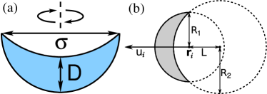
Figure 1: (a) The theoretical model of the colloidal bowl is the solid of revolution of a crescent around the axis indicated by the dashed line. The thickness of the double-walled bowl is denoted by $D$ and the diameter of the bowl by $\sigma$. (b) The bowls are defined using two spheres of radii $R_{1}$ and $R_{2}$, that are a distance of $L$ apart. The direction vector, $\mathbf{u}_{i}$ and the reference point of the particle, $\mathbf{r}_{i}$, (the dot in the center of the smaller sphere) are indicated.

II Methods

II.1 Model

We describe the model that we use to represent the bowls in more detail. Consider a sphere with a radius $R_{1}$ at the origin and a second sphere with radius $R_{2}>R_{1}$ at position $-L\mathbf{u}_{i}$, where $\mathbf{u}_{i}$ is the unit vector denoting the orientation of the bowl and $L>0$. The bowl is represented by that part of the sphere with radius $R_{1}$ that has no overlap with the larger sphere, see Fig. 1b. We have chosen the values for $L$ and $R_{2}$ such that the bowls are hemispherical (see appendix for explicit expressions for $L$ and $R_{2}$). We define the thickness of the bowls by $D=L-(R_{2}-R_{1})$, such that the model reduces to the surface of a hemisphere for $D=0$ and to a solid hemisphere for $D=R_{1}$. The volume of the particle is $\frac{\pi}{4}\,D\,(\sigma^{2}-D\sigma+\frac{2}{3}D^{2})$, where $\sigma\equiv 2R_{1}$ is our unit of length. The algorithm to determine overlap between our bowls is described in the appendix.

II.2 Fluid phase

We employ standard $NPT$ MC simulations to obtain the equation of state (EOS) for the fluid phase. In addition, we obtain the compressibility by measuring the fluctuations in the volume:

$$\frac{\langle V^{2}\rangle-\langle V\rangle^{2}}{\langle V\rangle}=\frac{k_{B}T}{\rho}\,\left(\frac{\partial\rho}{\partial P}\right)_{T},$$ (1)

where $\rho=N/V$ is the number density and the derivative of the pressure is taken at constant temperature is denoted by the subscript $T$. We determine the free energy at density $\rho_{1}$ by integrating the EOS from reference density $\rho_{0}$ to $\rho_{1}$:

$$\frac{F(\rho_{1})}{N}=\mu(\rho_{0})-\frac{P(\rho_{0})}{\rho_{0}}+\int_{\rho_{0}}^{\rho_{1}}\frac{P(\rho)}{\rho^{2}}d\rho$$ (2)

where the chemical potential $\mu(\rho_{0})$ is determined using the Widom particle insertion method Widom (1963), and $P(\rho_{0})$ is determined by a local fit to the EOS.

To investigate the structure of the fluid phase, we measure the positional correlation function Veerman and Frenkel (1992),

$$g_{c}(z)=\frac{1}{N\rho A_{\text{col}}}\langle\sum_{i=1}^{N}\sum_{j=1}^{N_{\text{col}}(i)}\delta(\mathbf{r}_{ij}\cdot\mathbf{u}_{i}-z)\rangle,$$ (3)

where the sum over $j$ runs over $N_{\text{col}}(i)$ particles in a column of radius $\sigma/2$ with orientation $u_{i}$ centered around particle $i$, and where the area of the column is denoted by $A_{\text{col}}=\pi\sigma^{2}/4$. At sufficiently high pressure the particles stack on top of each other to form disordered worm-like piles which resemble the stacks observed in the experiments Marechal et al. (2010). As the stacks have a strong tendency to buckle, we cannot use $g_{c}(z)$ to determine the length of the stacks. We therefore determine the stack size distribution using a cluster criterion. Particle $i$ and $j$ belong to the same cluster if

$$|\mathbf{r}_{ij}+(\zeta D/2+\sigma/4)(\mathbf{u}_{j}-\mathbf{u}_{i})| < \sigma/2\quad\text{and}$$

$$\mathbf{u}_{i}\cdot\mathbf{u}_{j} > 0,$$ (4)

and where the first condition has to be satisfied for $\zeta=-1$, $0$ or $1$ and $\mathbf{r}_{ij}=\mathbf{r}_{j}-\mathbf{r}_{i}$, with $\mathbf{r}_{i}$ denoting the center of the sphere with radius $R_{1}$ of particle $i$, see Fig. 1b. If both conditions are satisfied, particle $j$ is just above ($\zeta=1$) or below ($\zeta=-1$) particle $i$ in the stack, or, when the stack is curved, particle $j$ can be next to particle $i$ ($\zeta=0$). We now define the cluster distribution as the fraction of particles that belongs to a cluster of size $n$: $\mathcal{P}_{\text{stack}}(n)\equiv nN_{n}/N$, where $N_{n}$ is the number of clusters of size $n$. We checked that the cluster size distribution does not depend sensitively to the choice of parameters in Eq. (4).

II.3 Columnar phases

We also perform $NPT$ Monte Carlo simulations of the columnar phase using a rectangular simulation box with varying box lengths in order to relax the inter-particle distance in the $z$ direction, along the columns, independently from the lattice constant in the horizontal direction. The difference between the free energy of the columnar phase at a certain density and the free energy of the fluid phase at a lower density is determined using a thermodynamic integration technique Bates and Frenkel (1998). We apply a potential which couples a particle to its column:

$$\Phi_{\mathrm{hex}}(\mathbf{r}^{N},\lambda)=\lambda\sum_{i=1}^{N}\cos(2\pi N_{x}x_{i}/L_{x})\sin(\pi N_{y}y_{i}/L_{y}),$$ (5)

where $x_{i}$ and $y_{i}$ are the $x$ and $y$ components respectively of $\mathbf{r}_{i}$, $N_{\alpha}$ is the number of columns in the $\alpha$ direction and $L_{\alpha}$ is the size of the box in the $\alpha$ direction. In our simulations, we calculate Eq. (5) while fixing the center of mass. To do so efficiently, we first calculate all four combinations

$$\lambda\sum_{i=1}^{N}\mathrm{trig1}(2\pi N_{x}x_{i}/L_{x})\mathrm{trig2}(\pi N_{y}y_{i}/L_{y})$$ (6)

for $\mathrm{trig1}=\cos,\sin$ and $\mathrm{trig2}=\cos,\sin$. The change in these four expressions upon displacement of a single particle while keeping the center of mass fixed can be expressed in terms of single particle properties and the previous values of the expressions by using some basic trigonometry. In this way, $\Phi_{\mathrm{hex}}(\mathbf{r}^{N},\lambda)$, which is Eq. 6 for $\mathrm{trig1}=\cos$ and $\mathrm{trig2}=\sin$, can be calculated without performing the full summation over all particles in Eq. (6) every time we displace a particle. Unfortunately, this calculation requires the evaluation of many more trigonometric functions than the simple expression (5), but the extra computation time is negligible compared to the overlap check.

In addition to this positional potential, we also constrain the direction of the particle, using the potential

$$\Phi_{\text{ang}}(\mathbf{u}^{N},\lambda)=\lambda^{\prime}\sum_{i=1}^{N}u_{i,z},$$ (7)

where we used $\lambda^{\prime}=0.1\lambda$ and where $u_{i,z}$ is the $z$ component of $\mathbf{u}_{i}$. The thermodynamic integration path from the columnar phase to the fluid is as follows: We start from the columnar phase at a certain density $\rho_{2}$. Subsequently, we slowly turn on the two potentials, i.e. we increase $\lambda$ from 0 to $\lambda_{\mathrm{max}}$. Next, we integrate the equation of state to go from $\rho_{2}$ to $\rho_{1}$, while keeping $\lambda=\lambda_{\text{max}}$ fixed. During this step the columnar phase will only be stable below the coexistence density, if $\lambda_{\text{max}}$ is sufficiently high. We find that $\lambda_{\text{max}}=20k_{B}T$ suffices to guarantee stability of the columnar phase. Finally, fixing the density $\rho_{1}$, we gradually turn off the potentials, while integrating over $\lambda$ from $\lambda_{\text{max}}$ to 0. During this last step, the columnar phase melts continuously, provided that the density $\rho_{1}$ is low enough and that $\lambda$ is high enough to prevent melting during the density integration step. The resulting free energy difference between the columnar phase and fluid phase is given by

$$F_{\text{col}}(\rho_{2})-F_{\text{fluid}}(\rho_{1})=\\ \int_{0}^{\lambda_{\text{max}}}\big{\langle}\Phi_{\text{hex}}(\mathbf{r}^{N},\lambda)/\lambda+\Phi_{\text{ang}}(\mathbf{u}^{N},\lambda)/\lambda\big{\rangle}\big{|}_{\rho=\rho_{1}}+\\ \int_{\rho_{1}}^{\rho_{2}}d\rho\left.\frac{NP(\rho)}{\rho^{2}}\right|_{\lambda=\lambda_{\text{max}}}\\ -\int_{0}^{\lambda_{\text{max}}}\big{\langle}\Phi_{\text{hex}}(\mathbf{r}^{N},\lambda)/\lambda+\Phi_{\text{ang}}(\mathbf{u}^{N},\lambda)/\lambda\big{\rangle}\big{|}_{\rho=\rho_{2}}$$ (8)

The positional potential (5) is designed to stabilize a hexagonal array of columns, but, strictly speaking, it does not have the hexagonal symmetry of the columnar phase, since it is not invariant under a 60 degrees rotation of the whole system around a lattice position. However, we find that replacing Eq. (5) by a positional potential that does have this symmetry, does not have a significant effect on the free energy difference.

A second type of columnar phase can be constructed by flipping half of the bowls. In this way we obtain alternating vertical sheets (i.e. rows of columns) of bowls that point upwards and sheets of bowls that point downwards, we will refer to this phase as the inverted columnar phase. We calculate the free energy of this phase using the method described above, with the modification that the angular potential now reads,

$$\Phi_{\text{ang}}(\mathbf{u}^{N},\lambda)=\lambda^{\prime}\sum_{i}u_{i,z}^{2}.$$ (9)

This potential could also have been used for the non-inverted columnar phase, and we have found that the result of the free energy integration for the columnar phase is the same whether we use Eq. (9) or Eq. (7).

II.4 Crystals

II.4.1 Packing

As the crystal phases of the bowls are not known a priori, we developed a novel pressure annealing method to obtain the possible crystal phases Filion et al. (2009), which we named after the thermal annealing technique commonly used to find energy minima. Fully variable box shape $NPT$ simulations were performed on system of only 2-6 particles. By construction, the final configuration of such a simulation is a crystal, where the unit cell is the simulation box. One cycle of such a simulation consists of the following steps: We start at a pressure of $10k_{B}T/\sigma^{3}$. Subsequently, we run a series of simulations, where the pressure increases by a factor of ten each run: $P\sigma^{3}/k_{B}T=10,100,\ldots,10^{6}$. At the highest pressure ($10^{6}k_{B}T/\sigma^{3}$) we measure the density and angular order parameters, $S_{1}\equiv\|\langle\mathbf{u}_{i}\rangle\|$ and $S_{2}\equiv\lambda_{2}$, where $\lambda_{2}$ is the highest eigenvalue of the matrix whose components are $Q_{\alpha_{\beta}}=\frac{3}{2}\langle u_{i\alpha}u_{i\beta}\rangle-\frac{1}{2}\delta_{\alpha\beta}$, where $\alpha,\beta=x,y,z$. We store the density if it is the highest density found so far for these values of $S_{1}$ and $S_{2}$. We ran 1000 of such cycles for each aspect ratio, which is enough to visit each crystal phase multiple times. After completing the simulations, we tried to determine the lattice parameters of the resulting crystal by hand. Although this last step is not necessary, it is convenient to have analytical expressions for the lattice vectors and the density. The pressure annealing runs were performed for $D/\sigma=0.1,0.15,\ldots,0.5$. For many of the crystals, we were not able to find analytical expressions for the lattice parameters. For these crystals, we obtain the densities of the close packed crystals for intermittent values of $D$ by averaging the density in single simulation runs at a pressure of $10^{6}k_{B}T/\sigma^{3}$. The initial configurations for the value of $D$ of interest were obtained from the final configurations of the pressure annealing simulations for another value of $D$ by one of the following two methods, depending on whether we needed to decrease or increase $D$: When decreasing $L$ no overlaps are created so the final configuration of the simulation for the previous value of $L$ can be used as initial configuration. On the other hand, increasing $L$ results in an overlap, which is removed by scaling the system uniformly. Subsequently, the pressure is stepwise increased from 1000$k_{B}T/\sigma^{3}$ to $10^{6}k_{B}T/\sigma^{3}$, by multiplying by 10 each step.

II.4.2 Free energies

We calculate the free energy of the various crystal phases by thermodynamic integration using the Einstein crystal as a reference state Frenkel and Smit (2002). The Einstein integration scheme that we employ here is similar to the one that was used to calculate the free energies of crystals of dumbbells in Ref. Marechal and Dijkstra (2008). We briefly sketch the integration scheme here and discuss the modifications that we applied. We couple both the positions and the direction of the particles with a coupling strength $\lambda$, such that for $\lambda\rightarrow\infty$, the particles are in a perfect crystalline configuration. First, we integrate $\partial F/\partial\lambda$ over $\lambda$ from zero to a large but finite value for $\lambda$. Subsequently we replace the hard-core particle–particle interaction potential by a soft interaction, where we can tune the softness of the potential by the interaction strength $\gamma$. We integrate over $\partial F/\partial\gamma$ from a system with essentially hard-core interaction (high $\gamma=\gamma_{\text{max}}$), to an ideal Einstein crystal ($\gamma=0$). Some minor alterations to the scheme of Ref. Marechal and Dijkstra (2008) were introduced, which were necessary, because of the different shape of the particle. For the coupling of the orientation of bowl $i$, i.e., $\mathbf{u}_{i}$, to an aligning field, we have to take into account that the bowls have no up down symmetry, while the dumbbells are symmetric under $\mathbf{u}_{i}\rightarrow-\mathbf{u}_{i}$. The potential energy function that achieves the usual harmonic coupling of the particles to their lattice positions, as well as the new angular coupling, reads:

$$\beta U({\bf r}^{N},{\bf u}^{N};\lambda)=\\ \lambda\sum_{i=1}^{N}({\bf r}_{i}-{\bf r}_{0,i})^{2}/\sigma^{2}+\sum_{i=1}^{N}\lambda(1-\cos(\theta_{i0})),$$ (10)

where ${\bf r}_{i}$ and ${\bf u}_{i}$ denote, respectively, the center-of-mass position and orientation of bowl $i$ and ${\bf r}_{0,i}$ the lattice site of particle $i$, $\theta_{i0}$ is the angle between $\mathbf{u}_{i}$ and the ideal tilt vector of particle $i$, and $\beta=1/k_{B}T$. The Helmholtz free energy Marechal and Dijkstra (2008) of the noninteracting Einstein crystal is modified accordingly, but the only modification is the integral over the angular coordinates:

$$J(\lambda)=\int_{-1}^{1}e^{\lambda(x-1)}dx=\frac{1-e^{-2\lambda}}{\lambda}.$$ (11)

Although the shape of the bowls is more complex than that of the dumbbell, we can still use a rather simple form for the pairwise soft potential interaction:

$$\beta U_{\mathrm{soft}}({\bf r}^{N},{\bf u}^{N};\gamma)=\sum_{i<j}\beta\varphi({\bf r}_{i}-{\bf r}_{j},\mathbf{u}_{i},\mathbf{u}_{j},\gamma)$$ (12)

with

$$\beta\varphi({\bf r}_{j}-{\bf r}_{i},\mathbf{u}_{i},\mathbf{u}_{j},\gamma)=\\ \left\{\begin{array}[]{cc}\gamma(1-A(r_{ij}^{\prime}/\sigma_{\text{max}})^{2})&\text{if $i$ and $j$ overlap}\\ 0&\mathrm{otherwise}\end{array}\right.,$$ (13)

where $r_{ij}^{\prime}\equiv|\mathbf{r}_{j}-\mathbf{r}_{i}+\frac{\sigma-D}{2}(\mathbf{u}_{i}-\mathbf{u}_{j})|$ i.e. the distance between the “centers” of bowl $i$ and bowl $j$, $\sigma_{\text{max}}$ is the maximal $r_{ij}^{\prime}$ for which the particles overlap: $\sigma_{\text{max}}^{2}=\sigma^{2}+(\sigma-D)^{2}$, $A$ is an adjustable parameter that is kept fixed during the simulation at a value $A=0.5$, and $\gamma$ is the integration parameter. It was shown in Ref. Fortini et al. (2005) that in order to minimize the error and maximize the efficiency of the free energy calculation, the potential must decrease as a function of $r$ and must exhibit a discontinuity at $r$ such that both the amount of overlap and the number of overlaps decrease upon increasing $\gamma$. Here, we have chosen this particular form of the potential because it can be evaluated very efficiently in a simulation, although it does not describe the amount of overlap between bowls $i$ and $j$ very accurately. We checked that adding a term that tries to describe the angular behavior of the amount of overlap does not significantly change our results of the free energy calculations. Also, we checked that by employing the usual Einstein integration method (i.e. only hard-core interactions) at a relatively low density we obtained the same result as by using the method of Fortini et al.Fortini et al. (2005). Finally, we set the maximum interaction strength $\gamma_{\text{max}}$ to 200.

We perform variable box shape NPT simulations Parrinello and Rahman (1980) to obtain the equation of state for varying $D$. In these simulations not only the edge length changes, but also the angles between the edges are allowed to change. We employ the averaged configurations in the Einstein crystal thermodynamic integration. We calculate the free energy as a function of density by integrating the EOS from a reference density to the density of interest:

$$F(\rho_{1}^{*})=F(\rho_{0})+\int_{\rho_{0}}^{\rho_{1}}d\rho\left\langle\frac{NP(\rho)}{\rho^{2}}\right\rangle$$ (14)

III Results

Figure 2: The final configuration obtained from simulations at $P\sigma^{3}/k_{B}T=50$ and $D=0.3\sigma$ The colors denote different stacks.

III.1 Stacks

We perform standard Monte Carlo simulations in the isobaric-isothermal ensemble (NPT). Fig. 2 shows a typical configuration of bowl-shaped particles with $D=0.3~{}\sigma$ at $P\sigma^{3}/k_{B}T=50$, displaying stacking behavior typical for the worm-like phase.

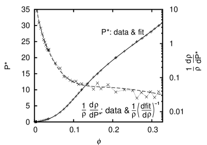
Figure 3: The equation of state for bowl-shape particles with $D=0.1\sigma$, reduced pressure $P^{*}=\beta P\sigma^{3}$ (left axis), and the reduced compressibility $\frac{1}{\rho}\,\frac{\partial\rho}{\partial P^{*}}$ on a log scale (right axis) as a function of packing fraction $\phi$. The points are data obtained from $NPT$ simulations. The solid line is a fit to the pressure; the dashed line is the corresponding reduced compressibility, $\frac{1}{\rho}\big{(}\frac{\partial\mathsf{fit}(\rho)}{\partial\rho}\big{)}^{-1}$.

The equation of state (EOS) of the fluid is somewhat peculiar: the pressure as a function of density is not always convex for all densities, although the compressibility does decrease monotonically with packing fraction $\phi$ for $D=0.1\sigma$, see Fig. 3, where the packing fraction is defined as $\phi=\frac{\pi D}{4}(\sigma^{2}-D\sigma+\frac{2}{3}D^{2})N/V$. This behavior persist for all $D\leq 0.2\sigma$, but for $D\geq 0.25\sigma$ the pressure is always convex. We investigate the origin of these peculiarities using $g_{c}(z)$, the positional correlation function along the director of a particle, which includes only the particles in a column around a particle, as defined in Eq. (3).

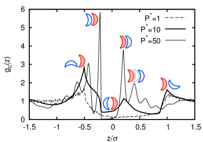
Figure 4: The pair correlation function, $g_{c}(z)$, of a fluid of bowl-shaped particles with $D=0.2\sigma$ as a function of the dimensionless inter-particle distance $z/\sigma$ along the axis of a reference bowl for various reduced pressures $P^{*}\equiv\beta P\sigma^{3}$. Only particles within a cylinder of diameter $\sigma$ around the bowl are considered, as indicated by the subscript ‘c’. We show typical two-particle configurations that contribute to $g_{c}(z)$ for $z/\sigma=-0.5,-0.2,0.2,0.4$ and $1$, where the filled bowls denote the reference particle, and the open bowls with thick outlines denote the other particle.

As can be seen from $g_{c}(z)$ in Fig. 4, the structure of the fluid changes dramatically as the pressure is increased. At $P^{*}\equiv\beta P\sigma^{3}=1$, the correlation function is typical for a low density isotropic fluid of hemispherical particles; no effect of the dent of the particles is found at low densities. The only peculiar feature of $g_{c}(z)$ for $P^{*}=1$ is that it is not symmetric around zero, but this is caused by our choice of reference point on the particle (see Fig. 1b), which is located below the particle if the particle points upwards. In contrast, at $P^{*}=10$ $g_{c}(z)$ already shows strong structural correlations. Most noteworthy is the peak at $z=D$, that shows that the fluid is forming short stacks of aligned particles. Also, note that the value of $g_{c}(z)$ is nonzero around $z=0$. This is caused by pairs of bowls that align anti-parallel and form a sphere-like object, as depicted in Fig. 4. Finally, at $P^{*}=50$ and higher, long worm-like stacks are fully formed and $g_{c}(z)$ shows multiple peaks at $z=Dn$ for both positive and negative integer values of $n$. Furthermore, at these pressures, there are no sphere-like pairs, as can be observed from the value of $g_{c}(0)$. The formation of stacks explains the peculiar behavior of the pressure: At low densities, the bowls rotate freely, which means that the pressure will be dominated by the rotationally averaged excluded volume. The excluded volume of two particles that are not aligned is nonzero, even for $D=0$, and gives rise to the convex pressure which is typical for repulsive particles. As the density increases and the bowls start to form stacks, the available volume increases, and the pressure increases less than expected, which can even cause the EOS to be concave. At even higher densities the worm-like stacks are fully formed, and the pressure is again a convex function of density for $D>0$, dominated by the excluded volume of locally aligned bowls. The excluded volume of completely aligned infinitely thin bowls is zero, and, therefore, the pressure increases almost linearly with density for $D=0$ when the stacks are fully formed.

Figure 5: The probability, $\mathcal{P}_{\text{stack}}(n)$, to find a particle in a stack of size $n$ for $D/\sigma=0.2,0.3$ and $0.4$ and $P\sigma^{3}/k_{B}T=50$

To quantify the length of the stacks we calculated the stack distribution as shown in Fig. 5. As can be seen from the figure, the length of the stacks is strongly dependent on $D/\sigma$. However, we have found that above a certain threshold pressure the distribution of stacks is nearly independent of pressure.

We investigated whether the worm-like stacks could spontaneously reorient to form a columnar phase. We increased the pressure in small steps of 1 $k_{B}T/\sigma^{3}$ from well below the fluid–columnar transition to very high pressures, where the system was essentially jammed. At each pressure, we ran the simulation for $4\cdot 10^{6}$ Monte Carlo cycles, where a cycle consists of $N$ particle and volume moves. These simulations show that the bowls with a thickness $D\geq 0.25\sigma$ always remained arrested in the worm-like phase, which is similar to the experimental observations Marechal et al. (2010). However, for $D/\sigma=0.1$ and $0.2$, we find that the system eventually transforms into a columnar phase in the simulations (see Fig. 6). This might be explained by the fact that the isotropic-to-columnar transition occurs at lower packing fractions for deeper bowls (smaller $D$), which facilitates the rearrangements of the particles into stacks and the alignment of the stacks into the columnar phase.

Figure 6: The final configuration of a simulation of bowls with $L=0.1D$ at $P\sigma^{3}/k_{B}T=38$. The gray values denote different columns.

III.2 Packing

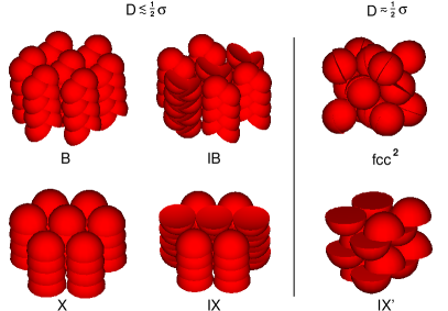
Figure 7: The various crystal phases that were considered as possible stable structures. Five of these were found using the pressure annealing method: X, IX, B, IB and IX’. X, IX, B and IB are densely packed structures for $D\lesssim 0.5\,\sigma$ and fcc² and IX’ are densely packed crystal structures for (nearly) hemispherical bowls ($D\simeq 0.5\,\sigma$).

We found six candidate crystal structures, denoted X,IX,IX’,B,IB and fcc², using the pressure annealing method. Snapshots of a few unit cells of these crystal phases are shown in Fig. 7. We will describe these crystal structures using the order parameters $S_{1}$, that measures alignment of the particles, and the nematic order parameter ($S_{2}$), that is nonzero for both parallel and anti-parallel configurations. Crystal structure X has $S_{1}\simeq 1$ and $S_{2}\simeq 1$, and the particles are stacked head to toe in columns. The lattice vectors are

$$\begin{array}[]{c}\displaystyle\mathbf{a_{1}}=\sigma\hat{x}\qquad\mathbf{a_{2}}=D\hat{z}\\[10.00002pt] \displaystyle\mathbf{a_{3}}=\frac{\sigma}{2}\hat{x}+\frac{1}{2}\sqrt{\sigma^{2}-D^{2}+2\sigma\sqrt{\sigma^{2}-D^{2}}}\;\hat{y}+\frac{D}{2}\hat{z},\end{array}$$ (15)

and the density is

$$\rho\sigma^{3}=\left[\frac{D\sigma}{2}\sqrt{\sigma^{2}-D^{2}+2\sigma\sqrt{\sigma^{2}-D^{2}}}\right]^{-1}.$$ (16)

The order parameters of the second crystal structure, are $S_{1}\simeq 0$ and $S_{2}\simeq 1$, which is caused by the fact that half of the particles point upwards, and the other half downwards. Further investigation shows that there are two phases with $S_{2}\simeq 1$ and $S_{1}\simeq 0$: one at low $D$ (IX) and one at $D\simeq\sigma/2$ (IX’). The structure within the columns of the first (IX) of these two structures is the same as for the X structure, but one half of these columns are upside down, like in the inverted columnar phase (in fact, the IX crystal melts into the inverted columnar phase). The lattice vectors of crystal structure IX are

$$\begin{array}[]{c}\displaystyle\mathbf{a_{1}}=\sigma\hat{x}\qquad\mathbf{a_{2}}=D\hat{z}\\[10.00002pt] \displaystyle\mathbf{a_{3}}=\frac{\sigma}{2}\hat{x}+\frac{1}{2}\sqrt{3\sigma^{2}-4D^{2}}\;\hat{y},\end{array}$$ (17)

and the density is

$$\rho\sigma^{3}=\left[\frac{D\sigma}{2}\sqrt{3\sigma^{2}-4D^{2}}\right]^{-1}.$$ (18)

The columns in the IX crystal are arranged in such a way that the rims of the bowls can interdigitate. The IX’ crystal can be obtained from the IX phase at $D=\sigma/2$ by shifting every other layer by some distance perpendicular to the columns, such that the particles in these layers fit into the gaps in the layers below or above. In this way a higher density than Eq. (18) is achieved. The columns of the third crystal phase (B) resemble braids with alternating tilt direction of the particles within each column. Because of this tilt $S_{1}$ and $S_{2}$ have values between 0 and 1, that depend on $D$. Furthermore, the inverted braids structure (IB), that has $0<S_{2}<1$ and $S_{1}=0$, can be obtained by flipping one half of the columns of the braid-like phase (B) upside down. These braid-like columns piece together in such a way that the particles are interdigitated. In other words, this phase is related to the B phase in exactly the same way as the IX phase is related to the X phase.

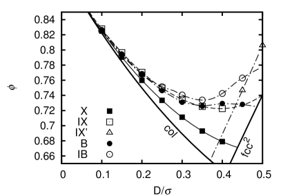
Figure 8: Packing diagram: maximum packing fraction ($\phi$) of various crystal phases as a function of the thickness ($D$) of the bowls. The points are the results of the pressure annealing simulations. The thin dot-dashed lines are obtained from the pressure annealing results by slowly increasing or decreasing $D$ as described in Sec. II.4, except for the IX phase (thin dashed line with open squares) and the X phase (thin solid line with filled squares), for which the packing fraction can be expressed analytically. The thick lines denote the packing fractions of the perfect hexagonal columnar phase (col) and the paired fcc phase (fcc²). Any points that lie below these lines are expected to be thermodynamically unstable (see text).

Finally, in the paired face-centered-cubic (fcc²) phase, pairs of hemispheres form sphere-like objects that can rotate freely and that are located at the lattice positions of an fcc crystal. The density at close packing is $2\sqrt{2}/\sigma^{3}$, i.e. twice the density of fcc.

In Fig. 8 the results of the pressure annealing method are shown, along with the known packing fraction of the perfect hexagonal columnar phase (col). Since the columnar phase has positional degrees of freedom and the fcc² phase has rotational degrees of freedom, we expect these phases to have a higher entropy (lower free energy) than any crystal phase with the same or lower maximum packing fraction whose degrees of freedom have all been frozen out. Therefore, any crystal structure with a packing fraction below the thick lines in Fig. 8 is most likely thermodynamically unstable. At first, we were unable to find the fcc² using the pressure annealing method as described in Sec. II.4. However, if we increase the pressure slowly to 100$k_{B}T/\sigma^{3}$ in simulations of 12 particles, we did observe the fcc² phase for hemispherical particles ($D=\sigma/2$). In these simulations at finite pressure, it is important to constrain the length of all box vectors such that they remain larger than say $1.5\sigma$. Otherwise the box will become extremely elongated, such that the particles can interact primarily with their own images. When a particle interacts with it is neighbors, the Gibbs free energy $G=F+PV$ decreases, because the volume decreases without any decrease in entropy due to restricted translational motion (if a particle moves, its image moves as well, so a particle translation will never cause overlap of the particle with its image). The decrease in Gibbs free energy is of course an extreme finite size effect, which should be avoided if we wish to predict the equilibrium phase behavior. For the pressure annealing simulations at very high pressures, these effects are not important, because the entropy term in the Gibbs free energy is small compared to $PV$.

phase	$D/\sigma$	$\rho_{\text{fluid}}\sigma^{3}$	$\rho_{\text{col}}\sigma^{3}$	$f_{\text{diff}}$
fluid–col	0	1.461	4.679	7.33272
phases	$D/\sigma$	$\phi_{\text{fluid}}$	$\phi_{\text{col}}$	$f_{\text{diff}}$
fluid–col	0.1	0.1780	0.2848	3.2630(7)
fluid–col	0.2	0.3116	0.4674	3.268(2)
fluid–col	0.3	0.3760	0.5193	3.802(1)
fluid–inv col	0.3	0.3760	0.5193	3.8155(8)
fluid–col	0.4	0.4440	0.5772	5.843

Table 1: Free energy differences, $f_{\mathrm{diff}}\equiv(F_{\text{col}}(\rho_{\text{col}})-F_{\mathrm{fluid}}(\rho_{\text{fluid}})/(Nk_{B}T)$, between the (inverted) columnar phase at density $\rho_{\text{col}}$ or packing fraction $\phi_{\text{col}}$ and the fluid phase at $\rho_{\text{fluid}}$ or $\phi_{\text{fluid}}$. In the column “phases”, “col” denotes the columnar phase and inverted columnar phase is abbreviated to “inv col”.

We did not attempt to find the columnar phase using the modified pressure annealing method, as we were only interested in finding candidate crystal structures. Furthermore, the columnar phase was already found in more standard simulations with a larger number of particles.

III.3 Free energies

In order to determine the regions of the stability of the fluid, the columnar phase and the six crystal phases, we calculated the free energies of all phases as explained in the Methods section. The results of the reference free energy calculations are shown in Tbls. 1 and 2.

phase	$D/\sigma$	$\phi$	$f_{\mathrm{exc}}$
IX	0.3	0.6669	15.505(4)
IB	0.3	0.6971	18.407(3)
IX	0.4	0.6177	12.52(1)
IB	0.4	0.6170	13.195(2)
IX	0.45	0.6768	17.918(2)
IB	0.45	0.6662	14.9873(4)
fcc2	0.45	0.6192	12.8591(5)
IX’	0.45	0.6950	18.170(5)
fcc2	0.5	0.5455	8.7673(7)
IX’	0.5	0.5597	10.854(3)

Table 2: Excess free energies, $f_{\mathrm{exc}}\equiv(F-F_{\mathrm{id}})/(Nk_{B}T)$, of the various crystal phases, where $F_{\mathrm{id}}$ is the ideal gas free energy. The various crystal phases are labeled as in Fig. 7.

We find that the columnar phase with all the particles pointing in the same direction is more stable than the inverted columnar phase, where half of the columns are upside down. However, the free energy difference between the two phases is only $0.013\pm 0.002k_{B}T$ per particle at $\phi=0.5193$ and $D=0.3\sigma$. Based on this small free energy difference we do not expect polar ordering to occur spontaneously. Similar conclusions, based on direct simulations, were already drawn in Ref. Ricci et al. (2008).

Figure 9: Dimensionless free energies $\beta F\,\sigma^{3}/V$ for hard bowls with $L=0.3\sigma$ and the fluid-columnar, columnar-IX and IX-IB coexistences, which were calculated using common tangent constructions. The columnar phases is denoted “col”. The irrelevant free energy offset is defined in such a way that the free energy of the ideal gas reads $\beta F/V=\rho(\log(\rho\sigma^{3})-1)$. The free energies of the various phases are so close, that they are almost indistinguishable.

The densely-packed crystal structures in Fig. 7 at $D\lesssim 0.3$, the worm-like fluid phase (Fig. 2) and the columnar phase (Fig. 6) show striking similarity in the local structure: in all these phases the bowls are stacked on top of each other, such that (part of) one bowl fits into the dent of another bowl. As a result, the free energies and pressures of the various phases, are often almost indistinguishable near coexistence. For this reason it was sometimes difficult to determine the coexistence densities for $D<0.3\sigma$. Exemplary free energy curves for the various stable phases consisting of bowls with $D=0.3\sigma$ are shown in Fig. 9.

III.4 Phase diagram

In Fig. 10, we show the phase diagram in the packing fraction $\phi$ - thickness $D/\sigma$ representation. The packing fraction is defined as $\phi=\frac{\pi D}{4}(\sigma^{2}-D\sigma+\frac{2}{3}D^{2})N/V$. For $D/\sigma\leq 0.3$, we find an isotropic-to-columnar phase transition at intermediate densities, which resembles the phase diagram of thin hard discs Veerman and Frenkel (1992). However, the fluid-columnar-crystal triple point for discs is at a thickness-to-diameter ratio of about $L/\sigma\sim 0.2-0.3$, while in our case the triple point is at about $D/\sigma\sim 0.3-0.4$. The shape of the bowls stabilizes the columnar phase compared to the fluid and the crystal phase. We find four stable crystal phases IX, IB, IX’ and fcc², while we had six candidate crystals. The two phases that were not stable are the X and B crystals, which are very similar to the stable IX and IB crystals respectively, except that X and B have considerable lower close packing densities. Therefore, one could have expected these phases to be unstable. On the other hand, we observe from the phase diagram, that IX is stable at intermediate densities for $0.25\sigma<D<0.45\sigma$, while IB packs better than IX. In other words, stability can not be inferred from small differences in packing densities.

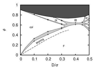
Figure 10: Phase diagram in the packing fraction ($\phi$) versus thickness ($D$) representation. The light gray areas are coexistence areas, while the state points in the dark gray area are inaccessible since they lie above the close packing line. IX, IB, IX’ and fcc² denote the crystals as shown in Fig. 7, “F” is the fluid and “col” is the columnar phase. The lines are a guide to the eye. Worm-like stacks were found in the area marked “worms” bounded from below by the dashed line. This line denotes the probability to find a particle in a cluster that consists of more than two particles, $\mathcal{P}_{\text{stack}}(n>2)=1/2$.

$D/\sigma$	phase 1	phase 2	$\rho_{1}\sigma^{3}$	$\rho_{2}\sigma^{3}$	$\beta P\sigma^{3}$	$\mu^{*}$
0	fluid	col	4.083	4.824	26.11	15.22

$D/\sigma$	phase 1	phase 2	$\phi_{1}$	$\phi_{2}$	$\beta Pd^{3}$	$\mu^{*}$
0.1	fluid	col	0.2778	0.3297	26.35	15.59
0.1	col	IX	0.8095	0.8104	$2.7\!\cdot\!10^{3}$	-
0.2	fluid	col	0.4096	0.4688	27.23	16.68
0.2	col	IX	0.7021	0.7108	325	-
0.3	fluid	col	0.5286	0.5472	49.52	26.13
0.3	col	IX	0.6864	0.6944	281.4	91.03
0.3	IX	IB	0.6117	0.6226	110.9	44.92
0.4	fluid	IB	0.6098	0.6455	105.9	51.06
0.45	fluid	IB	0.6026	0.6545	87.92	46.90
0.5	fluid	fcc2	0.4878	0.5383	28.34	22.10
0.5	fcc2	IX’	0.6870	0.7278	139.2	67.36

Table 3: Reduced densities, pressures and chemical potentials $\mu^{*}=\beta\mu-\ln(\Lambda_{t}^{3}\Lambda_{r}/\sigma^{3})$ of the coexisting phases for hard bowl-shaped particles with thickness $D$.

Almost all coexistence densities were calculated by employing the common tangent construction to the free energy curves, except for the col–IX coexistence at $D=0.1\sigma$ and $0.2\sigma$. At these values of $D$ the transition occurs at very high pressures, while the free energy of the columnar phase is calculated at the fluid–col transition, which occurs at a low pressure. To get a value for the free energy of the columnar phase we would have to integrate the equation of state up to these high pressures, accumulating integration errors. Furthermore, we expect the coexistence to be rather thin, which would further complicate the calculation. So, instead we just ran long variable box shape $NPT$ simulations to see at which pressure the IX phase melts into the inverted columnar phase. As the free energy difference between the inverted columnar phase and the columnar phase is small, we assume that this is the coexistence pressure for the col–IX transition, although technically it is only a lower bound. The density of the columnar phase at this pressure is determined using a local fit of the equation of state. All coexistences are tabulated in Tbl. 3. We draw a tentative line in the phase diagram to mark the transition from a structureless fluid to a worm-like fluid i.e. a fluid with many stacks. In a dense but structureless fluid, stacks of size 2 are quite probable, but larger stacks occur far less frequently. We calculate the probability to find a particle in a stack that contains more than 2 particles $\mathcal{P}_{\text{stack}}(n>2)=1-\mathcal{P}_{\text{stack}}(1)-\mathcal{P}_{\text{stack}}(2)$ and define the worm-like phase by the criterion $\mathcal{P}_{\text{stack}}(n>2)\geq 1/2$ in Fig. 10. We do not imply that the transition to the worm-like phase is a true thermodynamic phase transition; the transition is rather continuous. The type of stacks in the fluid changes from worm-like for $D=0.3\sigma$ to something resembling the columns in the braid-like crystals B and IB (see Fig. 7) for $D=0.4\sigma$. Therefore, the region of stability worm-like phase was ended at $D=0.35\sigma$, where there are similar amounts of braid-like and worm-like stacks.

IV Summary and discussion

We have studied the phase behavior of hard bowls in Monte Carlo simulations. We find that the bowls have a strong tendency to form stacks, but the stacks are bent and not aligned. We measured the equation of state and the compressibility in Monte Carlo $NPT$ simulations. The pressure we obtained from these simulations is concave for some range of densities for deep bowls. This is due to the increase in free volume when large stacks form. Using $g_{c}(z)$, the pair correlation function along the direction vector, we showed that the concavity of the pressure coincides with a dramatic change in structure from a homogeneous fluid to the worm-like fluid. We measured the three-dimensional stack length distribution in the simulations. When the pressure is increased slowly, the deep bowls spontaneously order into a columnar phase in our simulations. This poses severe restrictions on the thickness of future bowl-like mesogens (molecular or colloidal), which are designed to easily order into a globally aligned lyotropic columnar phase. We determined the phase diagram using free energy calculations for a particle shape ranging from an infinitely thin bowl to a solid hemisphere. We find that the columnar phase is stable for $D\leq 0.3\sigma$ at intermediate packing fractions. In addition, we show using free energy calculations that the stable columnar phase possesses polar order. However, the free energy penalty for flipping columns upside down is very small, which makes it hard to achieve complete polar ordering in a spontaneously formed columnar phase of bowls.

Appendix A Overlap algorithm

The overlap algorithm for our bowls checks whether the surfaces of two bowls intersect. Fig. 1 shows that the surface of the bowl consists of two parts. Part $p$ of the surface contains the part of the surface of the sphere of radius $R_{p}$, within an angle $\theta_{p}$ from the $z$-axis, where $p=1$ denotes the smaller sphere and the larger sphere is labeled $p=2$. We set $\theta_{1}=\pi/2$, to get a hemispherical outer surface. The edges of both surfaces have to coincide, such that our particles have a closed surface. Using this restriction $L$, $\theta_{2}$ and $R_{2}$ can all be expressed in terms of the radius of the smaller sphere, $R_{1}$, and the thickness of the bowl $D$, in the following way:

$$R_{2} = R_{1}+\frac{D^{2}}{2(R_{1}-D)}$$ (19)

$$\theta_{2} = \arcsin(R_{1}/R_{2})$$ (20)

$$L = R_{2}\cos(\theta_{2}).$$ (21)

Overlap occurs if either of the two parts of the surface of a bowl overlaps with either of the two parts of another bowl. So we have to check four pairs of infinitely thin (and not necessarily hemispherical) bowls, labeled $i$ and $j$, for overlap. The algorithm for two such surfaces that are equal in shape was already implemented by He and Siders He and Siders (1990) as part of their overlap algorithm for their “UFO” particles, which are defined as the intersection between two spheres. An equivalent overlap algorithm was used by Cinacchi and Duijneveldt Cinacchi and van Duijneveldt (2010) to simulate infinitely thin contact lense-like particles, but the overlap algorithm was not described explicitly. We can not use one of these algorithms, since the two parts of the surface of our particle are unequal in shape. Therefore, we implemented a slightly different version of the overlap algorithm, which we describe in the remainder of this section. In our overlap algorithm, the existence of a overlap or intersection between two infinitely thin bowls is checked in three steps.

• First, we check whether the full surfaces of the spheres intersect, i.e. $|R_{i}-R_{j}|<r_{ij}\equiv|\mathbf{r}_{j}-\mathbf{r}_{i}|<R_{i}+R_{j}$. If this intersection does not exist, there is no overlap, otherwise we proceed to the next step.

• Secondly, we determine the intersection of the surface of each sphere with the other bowl. The intersection of bowl $i$ with the sphere of bowl $j$ exists if

  $$|\omega_{ij}+\zeta\phi_{ij}|<\theta_{i}\\$$ (22)

  for $\zeta=1$ or $-1$, where

  $$\cos(\phi_{ij}) = \frac{R_{i}^{2}-R^{2}_{j}+r_{ij}^{2}}{2r_{ij}R_{i}}\ \mathrm{and}$$ (23)

  $$\cos(\omega_{ij}) = \frac{\mathbf{u}_{i}\cdot\mathbf{r}_{ij}}{r_{ij}}.$$ (24)

  see Fig. 11a.

  

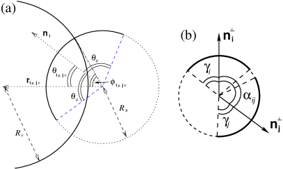
  Figure 11: The relevant lengths and angles which are used in the first and second steps (a) and in the third step (b) of the overlap algorithm. Shown are bowl $i$ and (part of) the sphere of bowl $j$ (a), the arcs of $i$ and $j$ and the circular intersection of the spheres of $i$ and $j$ (b). In (a) $\mathbf{r}_{ij}$ lies in the plane, while the plane of view in (b) is perpendicular to $\mathbf{r}_{ij}$. In this case, the sphere of particle $j$ overlaps with bowl $i$, but the arcs do not overlap, so particle $i$ and particle $j$ do not overlap.

  This intersection is an arc, which is part of the circle that is the intersection between the two spheres. If in fact this arc is a full circle and the other particle has a nonzero intersection, the particles overlap. This is the case when Eq. (22) holds for $\zeta=1$ and $\zeta=-1$. If, on the contrary, either of the two arcs does not exist, there is no overlap. Otherwise, if both arcs exist, but neither of them is a full circle, proceed to the next step.

• Finally, if the two arcs overlap there is overlap, otherwise the particles do not overlap. The arcs overlap if

  $$|\alpha_{ij}|<|\gamma_{i}|+|\gamma_{j}|,$$ (25)

  where

  $$\cos(\alpha_{ij}) = \frac{\mathbf{n}_{i}^{\perp}\cdot\mathbf{n}_{j}^{\perp}}{|\mathbf{n}_{i}^{\perp}||\mathbf{n}_{j}^{\perp}|}$$ (26)

  $$\cos(\gamma_{i}) = \frac{\cos(\theta_{i})-\cos(\phi_{ij})\cos(\omega_{ij})}{\sin(\phi_{ij})\sin(\omega_{ij})},$$ (27)

  where $\mathbf{n}_{i}^{\perp}=\mathbf{n}_{i}-(\mathbf{r}_{ij}\cdot\mathbf{n}_{i})\mathbf{r}_{ij}/r^{2}_{ij}$ and the expressions for $\gamma_{j}$ and $\mathbf{n}_{j}^{\perp}$ are equal to the expressions for $\gamma_{i}$ and $\mathbf{n}_{i}^{\perp}$ with $i$ and $j$ interchanged. The arcs together with the relevant angles are drawn in Fig. 11b.

The inequalities (22) and (25) are expressed in cosines and sines using some simple trigonometry. In this way no inverse cosines need to be calculated during the overlap algorithm.

For $D=0.5\sigma$ the bottom surface is a disk rather than an infinitely thin bowl. So the overlap check consists of bowl–bowl, bowl–disc and disc–disc overlap checks. For brevity, we will not write down the bowl–disk overlap algorithm, but it can be implemented in a similar way as the algorithm for bowl–bowl overlap described above. The disk–disk overlap algorithm was already implemented by Eppenga and Frenkel Eppenga and Frenkel (1984).

References

- Rabe et al. (2007) K. M. Rabe, M. Dawber, C. Lichtensteiger, C. H. Ahn, and J.-M. Triscone, in Physics of Ferroelectrics (Springer Berlin / Heidelberg, 2007) pp. 1–30.
- Ricci et al. (2008) M. Ricci, R. Berardi, and C. Zannoni, Soft Matter, 4, 2030 (2008).
- Sawamura et al. (2002) M. Sawamura, K. Kawai, Y. Matsuo, K. Kanie, T. Kato, and E. Nakamura, Nature, 419, 702 (2002).
- Simpson et al. (2004) C. D. Simpson, J. Wu, M. D. Watson, and K. Müllen, J. Mater. Chem., 14, 494 (2004).
- Xu and Swager (1993) B. Xu and T. M. Swager, J. Am. Chem. Soc., 115, 1159 (1993).
- Malthete and Collet (1987) J. Malthete and A. Collet, J. Am. Chem. Soc., 109, 7544 (1987).
- Rabideau and Sygula (1996) P. W. Rabideau and A. Sygula, Accounts of Chemical Research, 29, 235 (1996).
- Forkey et al. (1997) D. M. Forkey, S. Attar, B. C. Noll, R. Koerner, M. M. Olmstead, and A. L. Balch, J. Am. Chem. Soc., 119, 5766 (1997).
- Matsuo et al. (2004) Y. Matsuo, K. Tahara, M. Sawamura, and E. Nakamura, J. Am. Chem. Soc., 126, 8725 (2004).
- Sakurai et al. (2005) H. Sakurai, T. Daiko, H. Sakane, T. Amaya, and T. Hirao, J. Am. Chem. Soc., 127, 11580 (2005).
- Kawase and Kurata (2006) T. Kawase and H. Kurata, Chemical Reviews, 106, 5250 (2006).
- Cinacchi and van Duijneveldt (2010) G. Cinacchi and J. S. van Duijneveldt, J. Phys. Chem. Lett., 787 (2010).
- Zoldesi et al. (2006) C. I. Zoldesi, C. A. van Walree, and A. Imhof, Langmuir, 22, 4343 (2006).
- Charnay et al. (2003) C. Charnay, A. Lee, S.-Q. Man, C. E. Moran, C. Radloff, R. K. Bradley, and N. J. Halas, J. Chem. Phys. B, 107, 7327 (2003).
- Wang et al. (2004) X. D. Wang, E. Graugnard, J. S. King, Z. L. Wang, and C. J. Summers, nano lett., 4, 2223 (2004).
- Liu et al. (2005) J. Liu, A. I. Maaroof, L. Wieczorek, and M. B. Cortie, Adv. Mater., 17, 1276 (2005).
- Jagadeesan et al. (2008) D. Jagadeesan, U. Mansoori, P. Mandal, A. Sundaresan, and M. Eswaramoorthy, Angew. Chem. Int. Ed., 47, 7685 (2008).
- Love et al. (2002) J. C. Love, B. D. Gates, D. B. Wolfe, K. E. Paul, and G. M. Whitesides, nano lett., 2, 891 (2002).
- Hosein and Liddell (2007) I. D. Hosein and C. M. Liddell, Langmuir, 23, 8810 (2007).
- Higuchi et al. (2006) T. Higuchi, H. Yabu, and M. Shimomura, Colloids Surf. A, 284, 250 (2006).
- Lu et al. (2001) Y. Lu, Y. Yin, and Y. Xia, Adv. Mater., 13, 34 (2001).
- Marechal et al. (2010) M. Marechal, R. J. Kortschot, A. F. Demiroörs, A. Imhof, and M. Dijkstra, nano lett., 10, 1907 (2010).
- Widom (1963) B. Widom, J. Chem. Phys., 39, 2808 (1963).
- Veerman and Frenkel (1992) J. A. C. Veerman and D. Frenkel, Phys. Rev. A, 45, 5632 (1992).
- Bates and Frenkel (1998) M. A. Bates and D. Frenkel, Phys. Rev. E, 57, 4824 (1998).
- Filion et al. (2009) L. Filion, M. Marechal, B. van Oorschot, D. Pelt, F. Smallenburg, and M. Dijkstra, Phys. Rev. Lett., 103, 188302 (2009).
- Frenkel and Smit (2002) D. Frenkel and B. Smit, Understanding molecular simulation (Academic Press, 2002).
- Marechal and Dijkstra (2008) M. Marechal and M. Dijkstra, Phys. Rev. E, 77, 061405 (2008).
- Fortini et al. (2005) A. Fortini, M. Dijkstra, M. Schmidt, and P. P. F. Wessels, Phys. Rev. E, 71, 051403 (2005).
- Parrinello and Rahman (1980) M. Parrinello and A. Rahman, Phys. Rev. Lett., 45, 1196 (1980).
- He and Siders (1990) M. He and P. Siders, J. Chem. Phys., 94, 7280 (1990).
- Eppenga and Frenkel (1984) R. Eppenga and D. Frenkel, Mol. Phys., 52, 1303 (1984).