Exact and explicit probability densities for one-sided Lévy stable distributions

Abstract

We study functions $g_{\alpha}(x)$ which are one-sided, heavy-tailed Lévy stable probability distributions of index $\alpha$, $0<\alpha<1$, of fundamental importance in random systems, for anomalous diffusion and fractional kinetics. We furnish exact and explicit expressions for $g_{\alpha}(x)$, $0\leq x<\infty$, for all $\alpha\,=\,l/k<1$, with $k$ and $l$ positive integers. We reproduce all the known results given by $k\leq 4$ and present many new exact solutions for $k>4$, all expressed in terms of known functions. This will allow a ’fine-tuning’ of $\alpha$ in order to adapt $g_{\alpha}(x)$ to a given experimental situation.

Theoretical description of many collective physical systems which include special sort of disorder or randomness often requires a radical departure from classical diffusive behaviour. On the probabilistic level this signifies the appearance of distributions with non-conventional characteristics, like diverging mean and variance along with all integer moments different from zeroth one. In this context the prominent rôle plays the discovery of particular distributions with these properties, called now Lévy stable laws JPKahane95 , whose generic example is $g_{1/2}(x)~{}=~{}(2\sqrt{\pi}\,x^{3/2})^{-1}\,\exp(-1/4x)$, $x\geq 0$; the word ”stable” means here that the product of characteristic functions (cf) of two such laws is a cf of another law of the same type JPKahane95 . The general distribution of that type $g_{\alpha}(x)$ can be shown to possess the cf or the Laplace transform of the form JMikusinski59 ; HPollard46 ; WRSchneider86 :

$$\int_{0}^{\infty}e^{-p\,x}\,g_{\alpha}(x)\,dx\,=\,e^{-p^{\alpha}},\quad p>0\,,\,0<\alpha<1,$$ (1)

which is the well-known Kohlrausch-Williams-Watts function RSAnderssen04 or stretched exponential. Several independent proofs can be given that $g_{\alpha}(x)$ obeying Eq. (1) is positive JMikusinski59 ; HPollard46 ; IMSokolov00 .

The functions $g_{\alpha}(x)$ are ubiquitous in many fields of condensed and soft matter physics RMetzler04 ; PGDeGennes02 ; RHilfer02 , geophysics OSottolongo00 , meteorology MLagha07 , economics RNMantegna95 , fractional kinetics IMSokolov02 ; AVChechkin08 , etc. For instance, the value $\alpha=1/4$ is thought to describe mechanical and dielectric properties of glassy polymers JTBendler84 . It is also confirmed that the same value of $\alpha$ is relevant for a statistical description of subrecoil laser cooling FBardon02 ; FBardou94 . In general, numerous phenomena falling in the class of subdiffusion TKoren07 call for $g_{\alpha}(x)$, $\alpha<1$, in their theoretical description. On theoretical side, the Lévy stable distributions are essential tools in the study of random maps and resulting combinatorial structures PFlajolet . The actual use of Lévy stable type distributions has been hampered for subjective and objective reasons VVUchaikin99 ; VVUchaikin03 . The subjective ones include a certain reticence to use distributions with both mean and variance diverging. The main objective reason is a lack of knowledge of $g_{\alpha}(x)$ for most values of $\alpha$. The existing interpolation formulae JTBendler84 appear to be cumbersome to use.

It seems that obtaining explicit $g_{\alpha}(x)$ for arbitrary $0~{}<~{}\alpha~{}<~{}1$ constitutes a true challenge: only for a limited number of values of $\alpha$, i.e. $\alpha=1/2$ (s. $g_{1/2}(x)$ above), $1/4$ EBarkai01 , $1/3$ HScher75 , $2/3$ EWMontroll84 , and $3/4$ HScher75 the explicit forms of $g_{\alpha}(x)$ are known. The formal solution for arbitrary $\alpha$ WRSchneider86 ; RHilfer02 is only of a limited use as it requires series or asymptotic expansions, which may become problematic, especially for small $\alpha$.

The objective of this work is to present an universal formula for $g_{\alpha}(x)$, $\alpha=l/k$, with $k>l$ positive integers, which is exact and explicit. It reproduces all the known cases enumerated above, and yields an infinity of new solutions for $k>4$, of which we quote, for the first time, several instances.

Eq. (1) for $\alpha=l/k$ can be inverted giving

$$g_{l/k}(x)\,=\,\frac{\sqrt{kl}}{(2\pi)^{(k-l)/2}}\,\frac{1}{x}\,G^{k,0}_{l,k}\left(\frac{l^{l}}{k^{k}\,x^{l}}\,\Big{|}\,^{\Delta(l,0)}_{\Delta(k,0)}\right),$$ (2)

valid for all $x\geq 0$, where $G^{m,n}_{p,q}\left(z|^{(a_{p})}_{(b_{q})}\right)$ is the Meijer $G$ function OIMarichev83 ; APPrudnikov92 and $\Delta(k,a)=\frac{a}{k},\frac{a+1}{k},\ldots,\frac{a+k-1}{k}$ is a special list of $k$ elements. Eq. (2) is listed without proof as a special case for $\nu=0$ and $a=1$ of formula 2.2.1.19, in vol. 5 of APPrudnikov92 . The detailed demonstration of Eq. (2) with a combined use of Laplace and Mellin transforms will be given elsewhere. It turns out that the r. h. s. of Eq. (2) is a finite sum of $k-1$ generalized hypergeometric functions of type ${}_{p}F_{q}\left({}^{(a_{p})}_{(b_{q})}\big{|}z\right)$ APPrudnikov92 :

$$g_{l/k}(x)=\sum_{j=1}^{k-1}\frac{b_{j}(k,l)}{x^{1+j\,\frac{l}{k}}}\,\,_{l+1}F_{k}\left({}^{1,\Delta(l,\,1+j\,l/k)}_{\quad\Delta(k,j+1)}\Big{|}(-1)^{k-l}\frac{l^{l}}{k^{k}\,x^{l}}\right),$$ (3)

where $b_{j}(k,l)$ are numerical coefficients given by

$$b_{j}(k,l)=\frac{l^{jl/k}\,\sqrt{kl}}{k^{j}\,(2\pi)^{(k-l)/2}}\,\frac{\left[\prod_{i=1}^{j-1}\Gamma\left(\frac{i-j}{k}\right)\right]\,\left[\prod_{i=j+1}^{k-1}\Gamma\left(\frac{i-j}{k}\right)\right]}{\prod_{i=1}^{l-1}\Gamma\left(\frac{i}{l}-\frac{j}{k}\right)},$$ (4)

where $\Gamma(y)$ is Euler’s gamma function. Eq. (3) is the exact implementation of the program outlined in the fundamental work of Scher and Montroll HScher75 , in which it was conjectured that $g_{l/k}(x)$ can be expressed in terms of ${}_{p}F_{q}$’s. However in HScher75 actually only one new instance $g_{3/4}(x)$ was written down. Our formula Eq. (3), after appropriate reductions in ${}_{p}F_{q}$’s, see below, gives all exactly known cases mentioned above VVUchaikin99 ; VVUchaikin03 ; EBarkai01 ; HScher75 , with $g_{1/4}(x)$ EBarkai01

$$g_{1/4}(x) = \frac{b_{1}(4,1)}{x^{5/4}}\,_{0}F_{2}\left({}^{\,\,\,-}_{1/2,3/4}\Big{|}\frac{-1}{4^{4}x}\right)+\frac{b_{2}(4,1)}{x^{3/2}}$$

$$\times \,{}_{0}F_{2}\left({}^{\,\,\,-}_{3/4,5/4}\Big{|}\frac{-1}{4^{4}x}\right)+\frac{b_{3}(4,1)}{x^{7/4}}\,_{0}F_{2}\left({}^{\,\,\,-}_{5/4,3/2}\Big{|}\frac{-1}{4^{4}x}\right)$$

and offers an unlimited number of new solutions for $g_{l/k}(x)$, $k>4$, e.g.:

$$g_{p/5}(x)=\sum_{j=1}^{4}\,\frac{b_{j}(5,p)}{x^{1+jp/5}}\,_{p+1}F_{5}\left({}^{1,\Delta(p,1+j\,p/5)}_{\Delta(5,j+1)}\Big{|}\frac{p^{p}}{5^{5}x^{p}}\right),\quad$$ (6)

$p=1,\ldots,4$, see Table 1 for coefficients in Eqs. (Exact and explicit probability densities for one-sided Lévy stable distributions) and (6), etc.

j	1	2	3	4
$b_{j}(4,1)$	$\frac{1}{4\,\Gamma\left(\frac{3}{4}\right)}$	$\frac{-1}{4\sqrt{\pi}}$	$\frac{\sqrt{2}\,\Gamma\left(\frac{3}{4}\right)}{16\pi}$	—
$b_{j}(5,1)$	$\frac{\sqrt{5}\Gamma\left(\frac{1}{5}\right)}{20\pi\,B}$	$\frac{-\sqrt{5}\Gamma\left(\frac{2}{5}\right)}{20\pi\,A}$	$\frac{\sqrt{5}\Gamma\left(\frac{3}{5}\right)}{40\pi\,A}$	$\frac{-\sqrt{5}\Gamma\left(\frac{4}{5}\right)}{120\pi\,B}$
$b_{j}(5,2)$	$\frac{\sqrt{5}\cdot 2^{2/5}\Gamma\left(\frac{1}{5}\right)}{10\sqrt{\pi}\Gamma\left(\frac{3}{10}\right)\,B}$	$\frac{-\sqrt{5}\cdot 2^{4/5}\Gamma\left(\frac{2}{5}\right)}{10\sqrt{\pi}\Gamma\left(\frac{1}{10}\right)\,A}$	$\frac{-\sqrt{5}\cdot 2^{1/5}\Gamma\left(\frac{3}{5}\right)}{100\sqrt{\pi}\Gamma\left(\frac{9}{10}\right)\,A}$	$\frac{\sqrt{5}\cdot 2^{3/5}\Gamma\left(\frac{4}{5}\right)}{100\sqrt{\pi}\Gamma\left(\frac{7}{10}\right)\,B}$
$b_{j}(5,3)$	$\frac{3\sqrt{5}\cdot 3^{1/10}\Gamma\left(\frac{1}{5}\right)}{10\Gamma\left(\frac{2}{15}\right)\Gamma\left(\frac{7}{15}\right)\,B}$	$\frac{\sqrt{5}\cdot 3^{7/10}\Gamma\left(\frac{2}{5}\right)}{50\Gamma\left(\frac{4}{15}\right)\Gamma\left(\frac{14}{15}\right)\,A}$	$\frac{-3\sqrt{5}\cdot 3^{3/10}\Gamma\left(\frac{3}{5}\right)}{25\Gamma\left(\frac{1}{15}\right)\Gamma\left(\frac{11}{15}\right)\,A}$	$\frac{-7\sqrt{5}\cdot 3^{9/10}\Gamma\left(\frac{4}{5}\right)}{750\Gamma\left(\frac{8}{15}\right)\Gamma\left(\frac{13}{15}\right)\,B}$
$b_{j}(5,4)$	$\frac{4\cdot 2^{1/10}5^{-1/2}\sqrt{\pi}\Gamma\left(\frac{1}{5}\right)}{\Gamma\left(\frac{3}{10}\right)\Gamma\left(\frac{1}{20}\right)\Gamma\left(\frac{11}{20}\right)\,B}$	$\frac{6\cdot 2^{7/10}5^{-3/2}\sqrt{\pi}\Gamma\left(\frac{2}{5}\right)}{\Gamma\left(\frac{1}{10}\right)\Gamma\left(\frac{7}{20}\right)\Gamma\left(\frac{17}{20}\right)\,A}$	$\frac{14\cdot 2^{3/10}5^{-5/2}\sqrt{\pi}\Gamma\left(\frac{3}{5}\right)}{\Gamma\left(\frac{9}{10}\right)\Gamma\left(\frac{3}{20}\right)\Gamma\left(\frac{13}{20}\right)\,A}$	$\frac{11\cdot 2^{9/10}5^{-7/2}\sqrt{\pi}\Gamma\left(\frac{4}{5}\right)}{\Gamma\left(\frac{7}{10}\right)\Gamma\left(\frac{9}{20}\right)\Gamma\left(\frac{19}{20}\right)\,B}$

Table 1: Coefficients of Eqs. (Exact and explicit probability densities for one-sided Lévy stable distributions) and (6); $A=\sin(\pi/5)$ and $B=\sin(2\pi/5)$.

The symbol $\Delta(k,a)$ in Eq. (3) permits one to encode all the possible cases of $k$ and $l$ in a single formula. However we draw attention to the fact that cancellations will appear there due to the obvious identity ${}_{p+r}F_{q+r}\left({}^{(a_{p}),(\alpha_{r})}_{(b_{q}),(\alpha_{r})}\Big{|}\,x\right)=\,_{p}F_{q}\left({}^{(a_{p})}_{(b_{q})}\Big{|}\,x\right)$, where $(\alpha_{r})$ is an arbitrary sequence of $r$ parameters not equal to zero or to negative integers. Thus Eq. (Exact and explicit probability densities for one-sided Lévy stable distributions) is a sum of three ${}_{0}F_{2}$ functions, and likewise $g_{3/4}(x)$, which is not specified here, will be a sum of three ${}_{2}F_{2}$ functions, neatly confirming Eq. (C10) of HScher75 , etc. In this manner for any $l/k$, a closed form of $g_{l/k}(x)$ can be obtained from Eq. (3). However, only for $k\leq 3$ it can be written down in terms of standard special functions RSAnderssen04 ; HScher75 ; VVUchaikin99 ; VVUchaikin03 ; EWMontroll84 .

A heuristic indication of how Eq. (3) comes about can be obtained from the series representation for $g_{\alpha}(x)$ derived by Humbert PHumbert45 , discussed for example by Hughes BDHughes95 and used in PFlajolet . The series

$$g_{\alpha}(x)=\frac{1}{\pi}\,\sum_{j=1}^{\infty}\frac{(-1)^{j+1}}{j!\,x^{1+\alpha\,j}}\,\Gamma(1+\alpha\,j)\,\sin(\pi\,\alpha\,j)$$ (7)

is a convergent expansion valid for all $0<\alpha<1$ and $x>0$. For $\alpha=l/k$ the decomposition of the summation index $j$ modulo $k$ yields an equivalent representation of $g_{l/k}(x)$ as a sum of $k-1$ infinite series. The structure of the coefficients in each of these series involve gamma functions ratios of type $\Gamma(l\,i+\theta)/\Gamma(k\,i+\phi)$, where $i$ is the new summation index and $\theta$ and $\phi$ are simple functions of $k$ and $l$. The application of Gauss-Legendre multiplication formula to both of these gamma functions allows the identification of $\,{}_{p}F_{q}$’s in Eq. (3) and the extraction of coefficients $b_{j}(k,l)$ of Eq. (4).

The advantage of our solution, Eqs. (3) and (4) over Eq. (7) is clearly seen in practice, in conjunction with the use of computer algebra systems maple1 . Since in recent versions of these systems the hypergeometric functions $\,{}_{p}F_{q}$ as well as the Meijer G function are fully implemented, their use permits high-precision calculations. For reader’s convenience we give in syntax1 the Maple^® syntax for $g_{l/k}(x)$, see Eq. (2) above. Our experience indicates that for small $\alpha$ our results for small $x$ are more practical to use than the $x\to 0$ asymptotics given in JMikusinski59 . The reason is that there the region of applicability of Mikusiński’s asymptotic expansion JMikusinski59 shrinks to exceedingly small values of $x$. For example for $\alpha=1/20$, $g_{1/20}(0)=0$, but a huge peak in $g_{1/20}(x)$ appears already at $x\sim 10^{-14}$. In contrast, our formulae work fine for any $x$ in this region. In the opposite limit for $\alpha\apprle 1$ the Humbert expansion Eq. (7) is slowly convergent for $x<\alpha$ but approximation JMikusinski59 works well as then $g_{\alpha}(x)$ is very close to zero in a considerable region near $x=0$ (e.g. already for $\alpha=5/6$ the function $g_{5/6}(x)$ is practically equal to zero up to $x\approx 0.35$). Such a practically flat region for small $x$ can also be seen for $\alpha=4/5$, compare the curve III on Fig. 3.

In Fig. 1 we compare three distributions for $l/k=1/2$, $1/3$ and $1/4$. The salient feature for $l/k=1/4$ is the appearance of a sharp maximum for very small $x$ so that these three curves can be barely shown on the same scale. Analogously, for $l/k=1/5$ the maximum of $g_{1/5}(x)$ appears at $x_{0}(1/5)\approx 0.0002$ and the value $g_{1/5}(x_{0})\approx 25$. For $x<x_{0}(1/5)$ the values of $g_{1/5}(x)$ are very close to zero. As already mentioned above, for smaller values of $l/k$ this type of behaviour is even more pronounced and it explains a posteriori the difficulties encountered in devising approximations valid for small $l/k$ and small $x$ EWMontroll84 ; JTBendler84 . In Fig. 2 we present the comparison of several distributions for values $l/k\approx 1/2$. Here the ’sharpening’ of the distributions, as $l/k$ goes from $1/2$ to smaller values, is very clearly visible but is less dramatic than in Fig. 1. We present in Fig. 3 the new distributions $g_{p/5}(x)$ given by Eq. (6) for $p=2,3$ and $4$.

All these probability distributions share the following features: (a) $g_{\alpha}(x)\to 0$, for $x~{}\to~{}0$, where they present an essential singularity $\sim x^{\frac{-2+\alpha}{2(1-\alpha)}}\exp[-A(\alpha)x^{\frac{-\alpha}{1-\alpha}}]$, $A(\alpha)>0$ JMikusinski59 ; (b) $g_{\alpha}(x)\to B(\alpha)x^{-(1+\alpha)}$, for $x\to\infty$, $B(\alpha)>0$, indicating heavy-tailed asymptotics for large $x$; (c) all their fractional moments $M_{\alpha}(\mu)~{}=~{}\int_{0}^{\infty}x^{\mu}g_{\alpha}(x)dx=\Gamma(-\mu/\alpha)/[\alpha\,\Gamma(-\mu)]$, for real $\mu$, $-\infty<\mu<\alpha$, including $M_{\alpha}(0)=1$, are finite, and are infinite otherwise; (d) $g_{\alpha}(x)$ are unimodal with the maximum at $x_{0}(\alpha)$, and $x_{0}(\alpha)\to 0$ as $\alpha\to 0$.

The distributions $g_{\alpha}(x)$ constitute basic ingredients of all theories of anomalous diffusion where they are employed to produce solutions $P_{\alpha}(x,t)$ in space-time domain of various forms of the Fokker-Planck equations along with their fractional generalizations IMSokolov00 ; EBarkai01 . For instance in EBarkai01 $P_{\alpha}(x,t)$ is given as a convolution (called there inverse Lévy transform) of $\frac{d}{ds}\left[-g_{\alpha}(t/s^{1/\alpha})\right]$ with $P_{1}(x,t)$ being a normalized solution of the ordinary Fokker-Planck equation, see Eq. (1) in EBarkai01 . The explicit forms of $g_{\alpha}(x)$ presented here will permit further development of this ambitious approach.

The availability of $g_{l/k}(x)$ makes it possible to fully describe the long tail distributions of carrier transit times in amorphous materials such as As₂Se₃ and TNF-PVK. In fact in classic work HScher75 the measured values of $\alpha$ for these two materials were $\alpha=0.45$ and $\alpha=0.8$ respectively, compare Fig. 6 of HScher75 . These values were for a long time intractable theoretically. From now on, setting $\alpha=9/20$ and $\alpha=4/5$ in our Eqs. (2) and (3) directly provides the sought for framework for interpretation of these data. The appropriate distributions are presented as the curve II in Fig. (2), ($\alpha=9/20$) and the curve III in Fig. (3), ($\alpha=4/5$).

We believe that the exact forms of $g_{\alpha}(x)$ obtained in this work, along with their asymptotics for $x\to\infty$ and exact values of fractional moments, constitute a solid basis to extract a value of $\alpha$ best suited for an experimental situation at hand. Once it has been done, such description can be further ’fine-tuned’ by choosing values of $k$ and $l$ which would optimise the choice of $\alpha$. We hope that this approach will prove useful in practical applications.  

We thank Professor E. Barkai for kindly informing us about his results obtained in EBarkai01 .

The authors acknowledge support from Agence Nationale de la Recherche (Paris, France) under Program No. ANR-08-BLAN-0243-2.

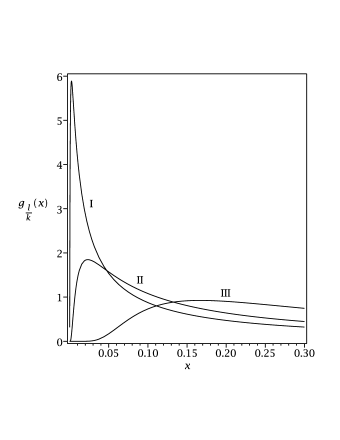
Figure 1: Comparison of $g_{l/k}(x)$: the curves I, II and III correspond to $l/k=1/4$ (s. Eq. (Exact and explicit probability densities for one-sided Lévy stable distributions)), $1/3$ and $1/2$, respectively.

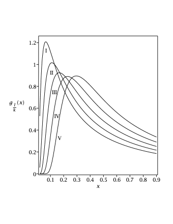
Figure 2: Comparison of $g_{l/k}(x)$: the curves I, II, III, IV and V correspond to $l/k=2/5,9/20,1/2,11/20$ and $3/5$, respectively. Calculations were performed using Eqs. (3) and (4).

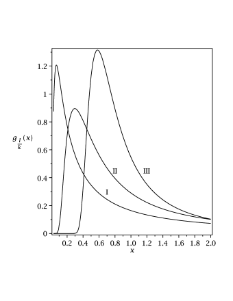
Figure 3: Comparison of $g_{l/k}(x)$: the curves I, II and III correspond to $l/k=2/5,3/5$ and $4/5$, respectively. Calculations were performed using Eq. (6).

References

- (1) J.-P. Kahane, in Lévy Flights and Related Topics in Physics, (Lecture Notes in Physics, vol. 450), edited by M.F. Shlesinger, G.M. Zaslavsky, and U. Frisch, (Springer, Berlin, 1995).
- (2) H. Pollard, Bull. Amer. Math. Soc. 52, 908 (1946).
- (3) J. Mikusiński, Studia Math. 18, 191 (1959).
- (4) W. R. Schneider, in Stochastic Processes in Classical and Quantum Systems (Lecture Notes in Physics, vol. 262), edited by S. Albeverio, G. Casati, and D. Merlini (Springer, Berlin, 1986).
- (5) R. S. Anderssen, S. A. Husain, and R. J. Loy, ANZIAM J. 45, C800 (2004).
- (6) I. M. Sokolov, Phys. Rev. E 63, 011104 (2000).
- (7) R. Metzler and J. Klafter, J. Phys. A 37, R161 (2004).
- (8) P.-G. de Gennes, Macromol. 35, 3785 (2002).
- (9) R. Hilfer, Phys. Rev. E 65, 061510 (2002).
- (10) O. Sottolongo-Costa, J. C. Antoranz, A. Posadas, F. Vidal, and A. Vazquez, Geophys. Res. Lett. 27, 1965 (2000).
- (11) M. Lagha and M. Bensebti, hal-00194153 (2007).
- (12) R. N. Mantegna and H. E. Stanley, Nature 376, 46 (1995).
- (13) I. M. Sokolov, J. Klafter, and A. Blumen, Phys. Today 55, 48 (2002).
- (14) A. V. Chechkin, V. Yu. Gonchar, R. Gorenflo, N. Korabel, and I. M. Sokolov, Phys. Rev. E 78, 021111 (2008).
- (15) J. T. Bendler, J. Stat. Phys. 36, 625 (1984).
- (16) F. Bardou, J.-P. Bouchaud, O. Emile, A. Aspect, and C. Cohen-Tannoudji, Phys. Rev. Lett. 72, 203 (1994).
- (17) F. Bardou, J.-P. Bouchaud, A. Aspect, and C. Cohen-Tannoudji, Lévy Statistics and Laser Cooling (Cambridge University Press, 2002).
- (18) T. Koren, J. Klafter, and M. Magdziarz, Phys. Rev. E 76, 031129 (2007).
- (19) P. Flajolet and R. Sedgewick, Analytic Combinatorics (Cambridge University Press, 2009).
- (20) V. V. Uchaĭkin, Zh. Éksp. Teor. Fiz. 115, 2113 (1999) [Sov. Phys. JETP 88, 1155 (1999)].
- (21) V. V. Uchaĭkin, Usp. Fiz. Nauk 173, 847 (2003) [Sov. Phys. Usp. 46, 821 (2003)].
- (22) E. Barkai, Phys. Rev. E 63, 046118 (2001).
- (23) H. Scher and E. W. Montroll, Phys. Rev. B 12, 2455 (1975).
- (24) E. W. Montroll and J. T. Bendler, J. Stat. Phys. 34, 129 (1984).
- (25) P. Humbert, Bull. Soc. Math. Fr. 69, 121 (1945).
- (26) B. D. Hughes, Random Walks and Random Environments, vol. 1 (Clarendon Press, Oxford, 1995).
- (27) We have made extensive use of Maple® in this work.
-
(28)
Here is the Maple® procedure LevyDist(k, l, x) used to calculate Eq. (2):
LevyDist := proc(k, l, x) simplify(convert( sqrt(k * l) * MeijerG([[],[seq(j1/l, j1 = 0..l-1)]] , [[seq(j2/k, j2 = 0..k-1)],[]], l^l /(k^k * x^l)) /(x*(2*Pi)^((k-l)/2)), StandardFunctions)); end; .
Analogous syntax can be given for Mathematica®. - (29) O. I. Marichev, Handbook of Integral Transforms of Higher Transcendental Functions. Theory and Algorithmic Tables (Ellis Horwood Ltd, Chichester, 1983).
- (30) A. P. Prudnikov, Yu. A. Brychkov, and O. I. Marichev, Integrals and Series, vols. 1-5 (Gordon and Breach, Amsterdam, 1992-1998).