Dynamical Fermion Masses Under the Influence of Kaluza-Klein Fermions and a Bulk Abelian Gauge Field

Abstract

The dynamical fermion mass generation on a 3-brane in the 5D space-time is discussed in a model with bulk fermions in interaction with fermions on the brane assuming the presence of a constant abelian gauge field component $A_{5}$ in the bulk. We calculate the effective potential as a function of the fermion masses and the gauge field component $A_{5}$. The masses can be found from the stationarity condition for the effective potential (the gap equation). We formulate the equation for the mass spectrum of the 4D–fermions. The phases with finite and vanishing fermion masses are studied and the dependence of the masses on the radius of the 5th dimension is analyzed. The influence of the $A_{5}$-component of the gauge field on the symmetry breaking is considered both when this field is a background parameter and a dynamical variable. The critical values of the $A_{5}$ field, the coupling constant and the radius are examined.

I Introduction

As originally proposed by Kaluza and Klein KK , an extra-dimensional space-time may be compactified to leave the 4-dimensional space-time as our real world. It was later demonstrated that the fundamental mass scale of the compactified space may be much smaller than the Planck mass Ant ; Ark1 . This stimulated intense studies of phenomenological evidences of extra-dimensional effects Han .Thus in the analysis of abe , bulk fermions were introduced in the 5D space-time interacting with fermions living on a 3-brane. The interaction between fermions generated as a result of the exchange of the Kaluza-Klein excited modes of the graviton may be expressed as effective four-fermion interaction Han that may lead to the dynamical generation of fermion masses Dob ; Chen .

On the other hand, there exists also the idea that the Higgs particle may originate from extra-dimensional components of gauge fields gaugehiggs . In this way, a Yukawa coupling to the 4D scalar, $A_{5}$, of the same strength as the gauge coupling, the so-called gauge-Yukawa unification, may also lead to a mass generation. A non-zero expectation value of $A_{5}$ then necessarily breaks the gauge and chiral symmetries of the underlying theory and $A_{5}$ thus plays the role of the Higgs field. This is a sort of radiative symmetry breaking Su , or Hosotani mechanism hosotani . Thus, it is the dynamical symmetry breaking by the four-fermion interaction which together with this Higgs-type mechanism generate the physical fermion mass spectrum.

In this paper, we will consider an extension of the fermion model abe describing the interaction of bulk fermions with fermions on a 3-brane in 5D space-time with one extra dimension compactified on a circle of radius $R$, by assuming the additional presence of a constant abelian gauge field component $A_{5}$ in the bulk. In particular, we will study chiral symmetry breaking and mass generation for light fermions under the combined influence of the effective four-fermion interactions and the bulk field component $A_{5}$ (in the following denoted as gauge field). For this aim, we first derive the effective potential $V_{\rm eff}(\sigma,A_{5})$ as function of the scalar (fermion condensate) field $\sigma$ and the constant field $A_{5}$ for the case of both periodic and antiperiodic boundary conditions of the bulk fermion field. The mean field values of these fields are then determined from the corresponding gap equations. On this basis the critical coupling constants $g_{c}$ for the chiral phase transition and the fermion condensate are numerically calculated and presented as functions of the compactification radius $R$ and $A_{5}$. Finally, we discuss the resulting fermion mass spectrum obtained from solving the corresponding eigenvalue equation for ground state and excited Kaluza-Klein states of fermions.

II The model

Two mechanisms of fermion mass generation are known: the dynamically generation of fermion masses and the Kaluza-Klein mechanism for generating masses of excited modes of the bulk fermions due to compactification. The mass of eventually existing Kaluza-Klein excited modes is expected to be of the order of TeV Cha . In the following we shall consider a 5D fermion model containing two types of fermion fields and a bulk gauge field $A_{M}$. One of the fermions, $\psi$, lives in the 5-dimensional bulk space, while the other one, $L$, exists only on a 3-brane which resides at a fixed point of the extra dimension. The interaction between these fermions is assumed to be given by a four-fermion term. Let us further suppose that the bulk fermion $\psi$ is charged and thus may interact with the bulk abelian gauge field $A_{M}$, whereas the fermion $L$ is neutral. Let us consider the vacuum averages $\langle A_{\mu}\rangle=0$, while $\langle A_{5}\rangle=A_{5}={\rm const}$. The presence of the constant potential $A_{5}$ then influences the dynamical mass generation arising from the four-fermion interaction. Moreover, for applying the $1/N_{f}$ expansion technique, fermions are assumed to be multiplets of a flavour $O(N_{f})$ group and thus to have $N_{f}$ flavour components.

The model is described by a straightforward extension of the Lagrangian studied in abe :

$$\mathcal{L}^{(5)}=\bar{\psi}i\Gamma^{M}D_{M}\psi+[\bar{L}i\gamma^{\mu}\partial_{\mu}L-\frac{g^{2}}{N_{f}}(\bar{\psi}\Gamma^{M}L)(\bar{L}\Gamma_{M}\psi)]\delta(y),$$ (1)

where $M=\mu,\,5;\,\,\mu=0,1,2,3$, $\Gamma^{M}=\{\gamma^{\mu},i\gamma^{5}\}$ and $D_{M}=\partial_{M}-ieA_{M}$ is the covariant derivative with $A_{M}$ being a bulk abelian gauge field . The fifth coordinate $y$ varies in the interval $[0,2\pi R]$.

Clearly, in the absence of the gauge field $A_{M}$ the Lagrangian is invariant under the $Z_{2}$ discrete “chiral” symmetry: $y\to-y$, $\psi(y)\to\gamma^{5}\psi(-y)$, $L(y)\to\gamma^{5}L(-y)$. The discrete symmetry thus prevents a mass term of the form $\bar{\psi}L$. To preserve this symmetry, the field $A_{M}$ should transform as $A_{\mu}(y)\to A_{\mu}(-y)$ and $A_{5}(y)\to-A_{5}(-y)$. Therefore the presence of the constant potential $A_{5}$ spontaneously breaks the chiral symmetry. In particular it is interesting to consider the influence of a constant $A_{5}$ on the dynamical mass generation of fermions.

As usually done in the case of NJL-type models (cf. e.g. EbR ), we next introduce an auxiliary (flavour-singlet) boson field $\sigma_{M}$ to obtain a linearized version of the above model Lagrangian

$$\mathcal{L}_{1}^{(5)}=\bar{\psi}i\gamma^{\mu}\partial_{\mu}\psi-\bar{\psi}\gamma^{5}\partial_{5}\psi+ie\bar{\psi}A_{5}\gamma^{5}\psi+[\bar{L}i\gamma^{\mu}\partial_{\mu}L+N_{f}\sigma^{M}\sigma_{M}^{*}+(g\sigma_{M}\bar{\psi}\Gamma^{M}L+h.c.)]\delta(y),$$ (2)

where summation over Dirac and flavour indices is implicitly included. In the following we shall consider the dynamical mass generation in the mean field approximation supposing that only the flavor-singlet field $\sigma_{5}$ acquires a non-vanishing vacuum expectation value $\langle\sigma_{5}\rangle=-\sigma$, whereas all the other irrelevant components of $\sigma_{M}$ vanish, $\langle\sigma_{\mu}\rangle=0$, $\mu=0,\ldots,3$. After performing the chiral rotation $\psi\to e^{i\frac{\pi}{4}\gamma^{5}}\psi$ and $L\to e^{i\frac{\pi}{4}\gamma^{5}}L$ one obtains

$$\mathcal{L}_{1}^{(5)}=i\bar{\psi}\not\!\partial\psi-i\bar{\psi}\partial_{5}\psi-eA_{5}\bar{\psi}\psi+[i\bar{L}\not\!\partial L-N_{f}|\sigma|^{2}+(g\sigma\bar{\psi}L+h.c.)]\delta(y).$$ (3)

Since the coordinate $y$ varies on the circle, the end points $y=0$ and $y=2\pi R$ must be identified. We adopt the general boundary condition for the fifth coordinate

$$\psi(x,y+2\pi R)=e^{i\pi\delta}\psi(x,y),$$ (4)

where the phase $\delta$ may have an arbitrary value in the range $0\leq\delta<2$. (Note that a change of the phase of the $\psi$-field does not affect the phase of the condensate $\sigma$ which exists only at $y=0$.) In particular, $\delta=0$ corresponds to a periodic boundary condition and $\delta=1$ to an antiperiodic one. Then we obtain the decomposition of the bulk fermion field into the Kaluza-Klein modes

$$\psi(x,y)=N\sum_{n=-\infty}^{\infty}\psi_{n}(x)e^{i\frac{y}{R}(n+\frac{\delta}{2})},$$ (5)

where $N$ is a normalization constant.

The Lagrangian (1) is invariant under the usual “small” gauge transformations

$$A_{M}(x,y) \to A_{M}(x,y)+\frac{1}{e}\partial_{M}\alpha(x,y),$$ (6)

$$\psi(x,y) \to e^{i\alpha(x,y)}\psi(x,y),$$ (7)

with periodic function $\alpha$: $\alpha(x,y+2\pi R)=\alpha(x,y)$.

In addition there are also “large” gauge transformations which satisfy the condition

$$\alpha(x,y+2\pi R)=\alpha(x,y)+2\pi l,\quad l=\pm 1,\pm 2,\ldots,$$ (8)

so that the boundary condition (4) for the transformed field $\psi$ is not violated. In particular, if we take $\alpha(x,y)=yl/R$, then the transformation of gauge fields yields:

$$A_{5}\to A_{5}+\frac{l}{eR},\quad l=\pm 1,\pm 2,\ldots.$$ (9)

Thus, an arbitrary constant potential $A_{5}$ cannot be gauged away when the fifth coordinate is compactified.

Integration over the coordinate $y$ yields the effective four-dimensional Lagrangian

$$\mathcal{L}^{(4)}\equiv\int_{0}^{2\pi R}dy\mathcal{L}_{1}^{(5)}=\sum_{n=-\infty}^{\infty}\left(i\bar{\psi}_{n}\not\!\partial\psi_{n}+(\frac{n+\delta/2}{R}-a)\bar{\psi}_{n}\psi_{n}\right)+i\bar{L}\not\!\partial L-N_{f}|\sigma|^{2}+\left(m\sum_{n=-\infty}^{\infty}\bar{\psi}_{n}L+h.c.\right),$$ (10)

where $a\equiv eA_{5}$ and $m\equiv Ng\sigma$. To obtain the properly normalized kinetic term, we chose $N=1/\sqrt{2\pi R}$.

III The mass spectrum

Let us next introduce matrix notations for the fermion fields $\Psi^{i}$ ($i=1,\ldots,N_{f}$) abe

$$(\Psi^{i})^{T}=\{L,\psi_{0},\psi_{1},\psi_{-1},\psi_{2},\psi_{-2},\ldots\}^{i},$$ (11)

and for the mass matrix $\mathcal{M}\equiv M\times I_{f}$, where $I_{f}$ is the unit operator in flavor space and

$$M\equiv\left(\begin{array}[]{ccccccc}0&m^{*}&m^{*}&m^{*}&m^{*}&m^{*}&\ldots\\ m&\frac{\delta}{2R}-a&0&0&0&0&\ldots\\ m&0&\frac{1}{R}+\frac{\delta}{2R}-a&0&0&0&\ldots\\ m&0&0&-\frac{1}{R}+\frac{\delta}{2R}-a&0&0&\ldots\\ m&0&0&0&\frac{2}{R}+\frac{\delta}{2R}-a&0&\ldots\\ m&0&0&0&0&-\frac{2}{R}+\frac{\delta}{2R}-a&\ldots\\ \vdots&\vdots&\vdots&\vdots&\vdots&\vdots&\ddots\\ \end{array}\right).$$ (12)

Then the effective Lagrangian can be written in the compact matrix form as follows

$$\mathcal{L}^{(4)}=\bar{\Psi}i\not\!\partial\Psi+\bar{\Psi}\mathcal{M}\Psi-N_{f}|\sigma|^{2}.$$ (13)

It should be noted that the fermions represented by $\Psi$ cannot be observed by themselves. Only the eigenstates of the mass matrix $M$ are observable fermions. Supposing that $\sigma_{5}$ acquires a non-vanishing vacuum expectation value $\langle\sigma_{5}\rangle=-\sigma$, we expect that the eigenvalues of the matrix $M$ with $m=Ng\sigma$ determine the masses of 4-dimensional fermions. They can be found in the following way. Consider the matrix

$$M-\lambda I\equiv\left(\matrix{-\lambda&m^{*}&m^{*}&m^{*}&m^{*}&m^{*}&\cdots\cr m&-\lambda-a+\frac{\delta}{2R}&0&0&0&0&\cdots\cr m&0&-\lambda-a+\frac{1}{R}+\frac{\delta}{2R}&0&0&0&\cdots\cr m&0&0&-\lambda-a-\frac{1}{R}+\frac{\delta}{2R}&0&0&\cdots\cr m&0&0&0&-\lambda-a+\frac{2}{R}+\frac{\delta}{2R}&0&\cdots\cr m&0&0&0&0&-\lambda-a-\frac{2}{R}+\frac{\delta}{2R}&\cdots\cr\vdots&\vdots&\vdots&\vdots&\vdots&\vdots&\ddots}\right).$$ (14)

Now we make use of the following identity Madelung

$$\left|\matrix{a_{11}&a_{12}&\cdots&a_{1n}&u_{1}&\cr a_{21}&a_{22}&\cdots&a_{2n}&u_{2}&\cr\vdots&\vdots&\vdots&\vdots&\vdots&\cr a_{n1}&a_{n2}&\cdots&a_{nn}&u_{n}&\cr v_{1}&v_{2}&\cdots&v_{n}&w&\cr}\right|\qquad=\qquad w|a_{ik}|\,-\,\sum_{i=1}^{n}\sum_{k=1}^{n}A_{ik}u_{i}v_{k},$$ (15)

where $A_{ik}$ is the algebraic supplement of $a_{ik}$. As a result, we have

$$\det(M-\lambda I)=\prod_{j=1}^{\infty}\left[(\lambda+a-\frac{\delta}{2R})^{2}-\left(\frac{j}{R}\right)^{2}\right]\left\{\lambda(\lambda+a-\frac{\delta}{2R})-|m|^{2}-2|m|^{2}(\lambda+a-\frac{\delta}{2R})^{2}\sum_{l=1}^{\infty}\frac{1}{(\lambda+a-\frac{\delta}{2R})^{2}-\left(\frac{l}{R}\right)^{2}}\right\}.$$ (16)

The eigenvalues of the matrix $M$ can then be obtained from the equation

$$\det(M-\lambda I)\,=\,0.$$ (17)

Finally, by using the summation formula

$$\sum_{n=1}^{\infty}\frac{1}{n^{2}-c^{2}}=\frac{1}{2c^{2}}-\frac{\pi}{2c}\cot{\pi c},$$ (18)

one can rewrite the eigenvalue equation as

$$\prod_{j=1}^{\infty}\left[(\lambda+a-\frac{\delta}{2R})^{2}-\left(\frac{j}{R}\right)^{2}\right]\left\{\lambda(\lambda+a-\frac{\delta}{2R})-|m|^{2}[\pi R(\lambda+a)-\frac{\pi\delta}{2}]\cot[\pi R(\lambda+a)-\frac{\pi\delta}{2}]\right\}=0.$$ (19)

It is easy to verify that $\lambda$-values satisfying $\lambda+a-\frac{\delta}{2R}=\frac{j}{R}$ ($j=0,1,2\ldots$) are not eigenvalues, since they are canceled by simple poles of the cotangent function in the curly brackets. Therefore the eigenvalues are determined from the transcendental equation

$$\lambda R=\pi|mR|^{2}\cot[\pi R(\lambda+a)-\frac{\pi\delta}{2}].$$ (20)

They define the finite masses of the 4-dimensional fermion eigenstates as functions of $m=Ng\sigma$ and $A_{5}$, if $\sigma_{5}$ and/or $A_{5}$ acquire non-vanishing vacuum expectation values.

IV The effective potential and gap equation

The generating functional of the system is given by

$$Z=\int[\mathcal{D}\bar{\Psi}][\mathcal{D}\Psi][\mathcal{D}\sigma][\mathcal{D}\sigma^{*}]\;e^{i\int d^{4}x\mathcal{L}^{(4)}}.$$ (21)

Next we perform the path-integration over the fermion fields $\Psi$,

$$Z=\int[\mathcal{D}\sigma][\mathcal{D}\sigma^{*}]\;e^{-iN_{f}\int d^{4}xV_{\mathrm{eff}}(\sigma)}.$$ (22)

As a result, we obtain in the mean field approximation (saddle point approximation in the leading order of the $1/N_{f}$ expansion) the effective potential

$$V_{\mathrm{eff}}(\sigma)=|\sigma|^{2}-\int\frac{d^{4}k}{i(2\pi)^{4}}\ln\det(M+I\!\not\!k).$$ (23)

Performing the Wick rotation we can rewrite the effective potential as an integral over the Euclidean momentum

$$V_{\mathrm{eff}}(\sigma)=|\sigma|^{2}-\frac{1}{8\pi^{2}}\int_{0}^{\Lambda^{2}}d(k_{E}^{2})\,k_{E}^{2}\ln\det(M^{2}+Ik_{E}^{2}),$$ (24)

where $\Lambda$ is the cutoff parameter.

To calculate the effective potential we used the following formula

$$\det(M^{2}+Ik_{E}^{2})=\det(M+iIk_{E})\det(M-iIk_{E})$$ (25)

and the explicit expressions for the determinants from formula (19). After some algebra we obtain:

$$V_{\mathrm{eff}}(\sigma,a) = |\sigma|^{2}-\frac{1}{4\pi^{2}}\int_{0}^{\Lambda}dx\,x^{3}\Biggl{\{}\ln\Bigl{(}x^{2}\left[\cosh 2\pi Rx-\cos(2\pi Ra-\pi\delta)\right]+2\pi Rx|m|^{2}\sinh 2\pi Rx$$ (26)

$$+ (\pi R|m|^{2})^{2}[\cosh 2\pi Rx+\cos(2\pi Ra-\pi\delta)]\Bigr{)}\Biggr{\}}.$$

The condensate $|\sigma|$ or the dynamical mass quantity $|m|=Ng|\sigma|$ is determined from the gap equation

$${\partial V_{\mathrm{eff}}(\sigma,a)\over\partial\sigma}\,\,=\,\,0,$$ (27)

or

$$\displaystyle 1-\frac{g^{2}}{4\pi^{2}}\int_{0}^{\Lambda}dx\,x^{3}\times$$ (28)

$$\displaystyle\frac{x\sinh 2\pi Rx+\pi R|m|^{2}[\cosh 2\pi Rx+\cos(2\pi Ra-\pi\delta)]}{x^{2}[\cosh 2\pi Rx-\cos(2\pi Ra-\pi\delta)]+2\pi Rx|m|^{2}\sinh 2\pi Rx+(\pi R|m|^{2})^{2}[\cosh 2\pi Rx+\cos(2\pi Ra-\pi\delta)]}=0.$$ (29)

A non-trivial solution exists only if the coupling constant exceeds its critical value $g_{c}$, which is obtained from the gap equation by setting $|\sigma|=0$:

$$1=\frac{g_{c}^{2}}{4\pi^{2}}\int_{0}^{\Lambda}dx\,x^{2}\frac{\sinh 2\pi Rx}{\cosh 2\pi Rx-\cos(2\pi Ra-\pi\delta)}.$$ (30)

It is easy to obtain from this equation the asymptotic value $g_{c}^{\ast}$ of the critical coupling at $R\to\infty$:

$$1=\frac{g_{c}^{\ast 2}\Lambda^{3}}{12\pi^{2}},$$ (31)

which evidently does not depend on the gauge potential $A_{5}$ nor on the phase factor $\delta$.

Fig. 1 shows the critical coupling constant as a function of the dimensionless radius $R\Lambda$ at different fixed values $a\Lambda^{-1}$ and as a function of the dimensionless potential $a\Lambda^{-1}$ at different fixed values $R\Lambda$ for the periodic boundary condition, i.e. $\delta=0$.

$\begin{array}[]{cc}\begin{@subfigure}\includegraphics[width=227.62204pt]{GR.eps}\end{@subfigure}&\begin{@subfigure}\includegraphics[width=227.62204pt]{Ga.eps}\end{@subfigure}\end{array}$

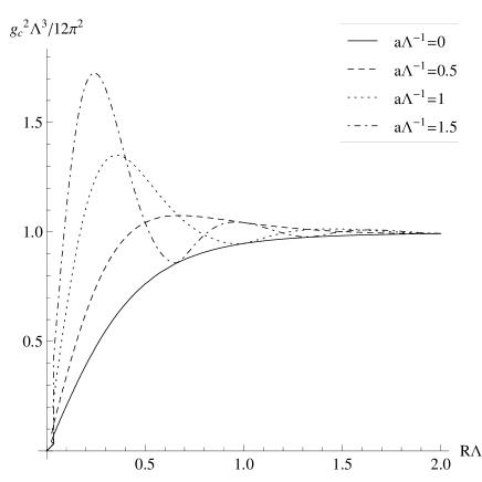
Figure 1: The critical coupling constant as function of $R\Lambda$ at different fixed values $a\Lambda^{-1}$ (a) and as function of $a\Lambda^{-1}$ at different fixed values $R\Lambda$ (b) for the periodic boundary condition $\delta=0$.

It is seen from the Fig. 1a that at small radius ($R\Lambda<1$) the critical coupling oscillates, whereas at large radius it tends to the asymptotic value (31) independent of the parameter $a$. In addition, the critical coupling oscillates as a function of the potential $A_{5}$ (see the Fig. 1b), however the amplitude of these oscillations becomes small for large radius.

It is also clear that if the coupling constant only slightly exceeds its critical value, the dynamical mass quantity $m$ is small and thus we can obtain light fermions in the considered model.

The solution of the gap equation for the mass quantity $m$ as function of the dimensionless compactification radius $R\Lambda$ for different fixed values of $a\Lambda^{-1}$ and as function of the dimensionless gauge field $a\Lambda^{-1}$ for different fixed values of $R\Lambda$ is depicted in Fig. 2 for $g^{2}\Lambda^{3}/12\pi^{2}=1.25$ and $\delta=0$.

$\begin{array}[]{cc}\begin{@subfigure}\includegraphics[width=227.62204pt]{mR.eps}\end{@subfigure}&\begin{@subfigure}\includegraphics[width=227.62204pt]{ma.eps}\end{@subfigure}\end{array}$

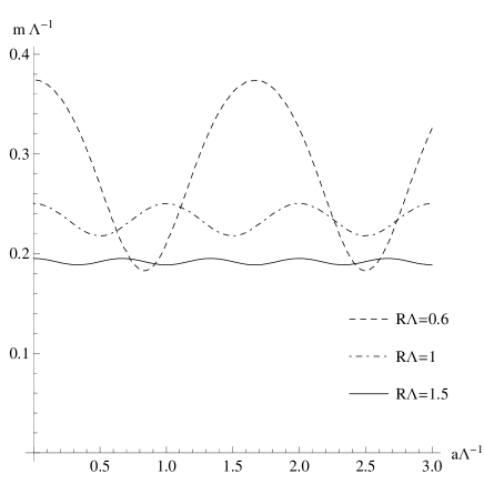
Figure 2: The fermion mass quantity $m$ as function of $R\Lambda$ at different fixed values $a\Lambda^{-1}$ (a) and as function of $a\Lambda^{-1}$ at different fixed values $R\Lambda$ (b) for $g^{2}\Lambda^{3}/12\pi^{2}=1.25$ and $\delta=0$.

It is seen that at large radius $R$ ($R\Lambda>1$) the dynamical quantity $m$ approaches its value corresponding to a vanishing gauge potential, $a=0$. Moreover, $m$ is an oscillating function of the gauge potential $a$.

There seem to exist two solutions for the mass quantity $m$ for $a\Lambda^{-1}=1$ or 1.5 as shown in Fig. 2. The physical reason of this is the oscillation of the critical coupling on Fig. 1a for $R\Lambda<1$. The curves for $a\Lambda^{-1}=1$ or 1.5 consist of two pieces, because at some values of $R\Lambda$ the critical coupling exceeds the fixed value $g^{2}\Lambda^{3}/12\pi^{2}=1.25$ (see Fig.1a) and therefore there is no solution of the gap equation for these values of $R\Lambda$.

V Dynamical A-field

Let us consider the gauge field component $a$ as a dynamical variable hosotani . Then the extremum of the effective potential is determined by the stationarity condition

$$\displaystyle\frac{\partial V_{\mathrm{eff}}}{\partial a}=-\frac{R}{2\pi}\int_{0}^{\Lambda}dx\,x^{3}\times$$

$$\times\displaystyle\frac{(x^{2}-(\pi R|m|^{2})^{2}\sin(2\pi Ra-\pi\delta)}{x^{2}[\cosh 2\pi Rx-\cos(2\pi Ra-\pi\delta)]+2\pi Rx|m|^{2}\sinh 2\pi Rx+(\pi R|m|^{2})^{2}[\cosh 2\pi Rx+\cos(2\pi Ra-\pi\delta)]}=0,$$ (32)

The extremum is evidently achieved at $2Ra-\delta=n$, where $n\in\mathbb{Z}$. The cases of even $n$ ($n=2k$) and odd $n$ ($n=2k+1$) should be considered separately, because they lead to different expressions for the effective potential. Therefore we have two types of solutions: $a=\frac{k}{R}+\frac{\delta}{2R}$ and $a=\frac{k}{R}+\frac{1+\delta}{2R}$, ($k=0,1,2,\ldots$). Recalling the large gauge transformation (9) it is clear that these two sets of solutions are equivalent to $a=\frac{\delta}{2R}$ and $a=\frac{1+\delta}{2R}$. Let us consider in the following only the cases of periodic and antiperiodic boundary conditions, i.e. $\delta=0$ and $\delta=1$. In the case $\delta=0$ we simply have two phases with trivial and nontrivial field $a$: $a=0$ and $a=\frac{1}{2R}$. It is easy to see that in the case of antiperiodic boundary condition these two phases just interchange. Therefore, in what follows we consider only the case of periodic boundary conditions, $\delta=0$.

To obtain the true vacuum of the model one needs to compare the minimum values of the potentials $V_{1}(\sigma)$ and $V_{2}(\sigma)$ which follow from the effective potential (26) by letting $a=\frac{\delta}{2R}$ and $a=\frac{1+\delta}{2R}$. The global minimum is realized at non-trivial values of $a$ depending on the coupling $g$ and radius $R$. The result of this comparison is presented in Fig. 3 where the critical curve which separates the phases with $a=0$ and $a=\frac{1}{2R}$ is depicted. The region above (below) the curve corresponds to the phases with $a=0$ ($a=\frac{1}{2R}$) for the periodic boundary condition and vice versa for the antiperiodic one.

Figure 3: The critical curve separates the phases with trivial and non-trivial $a$. The region above (below) the curve corresponds to $a=0$ ($a=\frac{1}{2R}$) for the periodic boundary condition and vice versa for the antiperiodic one.

Let us compare the dynamical mass generation for trivial and non-trivial $a$. The critical couplings for both phases are shown in Fig. 4a.

$\begin{array}[]{cc}\begin{@subfigure}\includegraphics[width=227.62204pt]{cc1}\end{@subfigure}&\begin{@subfigure}\includegraphics[width=227.62204pt]{m1}\end{@subfigure}\end{array}$

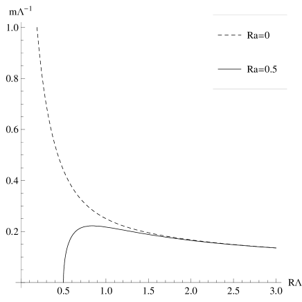
Figure 4: The critical coupling constant (a) and dynamical mass quantity $m$ as functions of the radius at $g^{2}\Lambda^{3}/12\pi^{2}=1.25$ (b).

In both cases the nontrivial solution for the dynamical mass quantity may exist only for those values of the coupling constants that lie above the appropriate critical curve. It is seen that at $a=0$ the critical curve starts from zero at $R\to 0$ and therefore even if the coupling is fixed in such a way that it is less than the asymptotic value (31) the dynamical mass can still be nonzero for small radius ($R\Lambda\lesssim 1$) (if $g>g_{c}^{\ast}$ the fermion mass exists at all radii of extra dimension). For $a=1/(2R)$ the critical coupling goes to infinity at $R\to 0$ and thus the gap equation has a nonzero solution only if $g>g_{c}^{\ast}$ and only for a sufficiently large radius. This situation is illustrated in Fig. 4b where the typical behavior of the dynamical mass quantity is represented as a function of the radius inside both phases at fixed coupling $g^{2}\Lambda^{3}/12\pi^{2}=1.25$.

Let us recall that the mass spectrum of 4-dimensional fermions is determined from (20). For $a=0$ we simply obtain

$$\lambda R=\pi|mR|^{2}\cot\pi R\lambda.$$ (33)

We are interested here in a light fermion with mass $\lambda\ll 1/R$. It can be easily shown that the lowest Kaluza-Klein mode in this case has the mass $\lambda=\pm m$. The dynamical mass $|m|$ is small ($|m|\ll 1/R$), if the coupling is close to its critical value.

When $a=(2R)^{-1}$ we have for the spectrum

$$\lambda R=\pi|mR|^{2}\cot\pi(R\lambda+{1\over 2}).$$ (34)

For $|\pi(R\lambda+{1\over 2})|\ll 1$ we have

$$\lambda R=-{1\over 4}\,-\,\sqrt{{1\over 16}+|mR|^{2}}\approx-{1\over 2}+O(|mR|^{2})\,\,\,{\rm for}\,\,\,|mR|^{2}\ll 1.$$

Therefore in this case we have $\lambda\approx-{1\over 2R}=-a$. Since the cotangent is periodical with the period $\pi$, we may rewrite (34) in the form

$$\lambda R=\pi|mR|^{2}\cot\pi(R\lambda-{1\over 2}),$$ (35)

with the corresponding approximate solution $\lambda\approx+{1\over 2R}=a$. It is seen that independently of any nonzero value of $|m|>0$ the lowest fermion mode is now massless: $\lambda=0$. The higher modes have the masses $\lambda\approx\pm{1\over 2R}=\pm a$, and other Kaluza-Klein modes have even higher masses $\lambda_{n}\approx\frac{n}{R}$.

VI Summary

In this paper we have studied the dynamical mass generation of fermions in a 5D model with one compact extra dimension and with bulk fermions in interaction with fermions living on a 3-brane under the influence of a constant gauge field component $A_{5}$. If $A_{5}$ is considered as a background parameter, then for sufficiently large radii the dynamical mass becomes independent of the gauge field and approaches its value corresponding to a vanishing gauge potential. Moreover, the dynamical mass is an oscillating function of the field component $A_{5}$ with an amplitude of oscillations that decreases with growing radius $R$.

On the other hand, if we consider the gauge potential as a dynamical variable, then it may acquire trivial or nontrivial values depending on the choice of the coupling constant $g$. In particular, it was demonstrated that for a vanishing gauge field and a coupling constant close to its critical value, it is possible to obtain a light fermion mode whose mass is lower than the inverse radius, which is in correspondence with the results of abe . However, if $A_{5}$ acquires a nonvanishing value, then the lowest fermion mode is massless independently of the dynamical mass $m$. Other possible modes have masses $\lambda\approx\pm{1\over 2R}=\pm a$, and higher Kaluza-Klein modes have even higher masses $\lambda_{n}\approx\frac{n}{R}$. The investigated interplay of the influence of Kaluza-Klein fermions and bulk gauge fields on the generation of dynamical masses of fermions living on a brane seems to us conceptually interesting and worth to be generalized to other, phenomenologically more realistic models.

References

- (1) Th. Kaluza, Sitzungsber. d. Preuss. Akad. d. Wiss. p.966 (1921); O. Klein, Zeitsch. f. Phys. 37, 895 (1926).
- (2) I. Antoniadis, Phys. Lett. B 246, 377 (1990); I. Antoniadis and K. Benakli, Phys. Lett. B 326, 69 (1994).
- (3) N. Arkani-Hamed, S. Dimopoulos and G. Dvali, Phys. Lett. B429, 263 (1998); Phys. Rev. D59, 086004 (1999); I. Antoniadis, N. Arkani-Hamed, S. Dimopoulos and G. Dvali, Phys. Lett. B 436, 257 (1998).
- (4) T. Han, J. D. Lykken and R-J. Zhang, Phys. Rev. D59, 105006 (1999).
- (5) H. Abe, H. Miguchi, and T. Muta, Mod.Phys.Lett., A15, 445 (2000).
- (6) B. A. Dobrescu, Phys. Lett. B461, 99 (1999).
- (7) H-C. Cheng, B. A. Dobrescu and C. T. Hill, Nucl. Phys. B 589, 249 (2000); A. B. Kobakhidze, hep-ph/9904203.
- (8) N. S. Manton, Nucl. Phys. B 158, 141 (1979); D. B. Fairlie, Phys. Lett. B 82, 97 (1979); J. Phys. G 5, L55 (1979); P. Forgacs and N. S. Manton, Commun. Math. Phys. 72, 15 (1980); S. Randjbar-Daemi, A. Salam and J. A. Strathdee, Nucl. Phys. B 214, 491 (1983).
- (9) R. Sundrum, arXiv:hep-th/0508134v2.
- (10) Y. Hosotani, Phys. Lett. B 126, 309 (1983); Annals Phys. 190, 233 (1989).
- (11) S. Chang, J. Hisano, H. Nakano, N. Okada and M. Yamaguchi, Phys. Rev. D62, 084025 (2000).
- (12) D.Ebert and H.Reinhardt, Nucl.Phys. B 271, 188 (1986); D.Ebert, H.Reinhardt and M.K. Volkov, Prog. Part. Nucl. Phys.33, 1 (1994).
- (13) E. Madelung, Die Mathematischen Hilfsmittel des Physikers, Springer-Verlag, 1957.