Statistical mechanics of Fofonoff flows in an oceanic basin
Abstract
We study the minimization of potential enstrophy at fixed circulation and energy in an oceanic basin with arbitrary topography. For illustration, we consider a rectangular basin and a linear topography which represents either a real bottom topography or the -effect appropriate to oceanic situations. Our minimum enstrophy principle is motivated by different arguments of statistical mechanics reviewed in the article. It leads to steady states of the quasigeostrophic (QG) equations characterized by a linear relationship between potential vorticity and stream function . For low values of the energy, we recover Fofonoff flows [J. Mar. Res. 13, 254 (1954)] that display a strong westward jet. For large values of the energy, we obtain geometry induced phase transitions between monopoles and dipoles similar to those found by Chavanis & Sommeria [J. Fluid Mech. 314, 267 (1996)] in the absence of topography. In the presence of topography, we recover and confirm the results obtained by Venaille & Bouchet [Phys. Rev. Lett. 102, 104501 (2009)] using a different formalism. In addition, we introduce relaxation equations towards minimum potential enstrophy states and perform numerical simulations to illustrate the phase transitions in a rectangular oceanic basin with linear topography (or -effect).
pacs:
05.20.-y Classical statistical mechanics - 05.45.-a Nonlinear dynamics and chaos - 05.90.+m Other topics in statistical physics, thermodynamics, and nonlinear dynamical systems - 47.10.-g General theory in fluid dynamics - 47.15.ki Inviscid flows with vorticity - 47.20.-k Flow instabilities - 47.32.-y Vortex dynamics; rotating fluidsI Introduction
The dynamics of the oceans is extremely complex due to nonlinear coupling across many scales of motion and the interplay between mean and fluctuating fields holloway . Although the oceans can be considered as “turbulent” in a classical sense, their dynamics also involves wavelike phenomena and coherent structures (vortices) like monopoles, dipoles or modons, tripoles… Furthermore, despite the permanent action of forcing (e.g. induced by the wind) and dissipation, the oceans present a form of global organization. This is revealed in the existence of strong jets like the Gulf Stream or the Kuroshio Current and in the observation of a large-scale oceanic circulation. In order to understand the dynamics of the oceans, one possibility is to develop numerical codes with increasing complexity. However, the results can be affected by the method used to parameterize the small scales. Furthermore, numerical simulations alone do not explain the phenomena observed. Therefore, in order to understand the physical output of such numerical simulations it can be useful to consider in parallel simple mathematical models that can be studied in great detail. These academic models can serve as a basis to develop general methods (e.g. statistical mechanics, kinetic theories) that can be relevant in more complicated situations.
Early models of wind-induced oceanic circulation have been developed by Stommel stommel and Munk munk but they are based on linearized equations and on an artificial concept of eddy viscosity. Alternatively, in a seminal paper, Fofonoff fofonoff neglects forcing and dissipation and studies the case of a steady free circulation in a closed ocean. He considers quasi geostrophic (QG) flows on the -plane, a common starting point for many dynamical studies in meteorology and oceanography. He furthermore assumes that the ocean has reached a steady state characterized by a linear relationship between potential vorticity and stream function (here, denotes the topography and the ordinary -effect corresponds to ). Finally, he considers an asymptotic regime of low energy and provides a simple analytical solution representing a westward jet with a recirculation at the boundary. This solution is now called Fofonoff flow pedlosky . Numerical simulations starting from a random initial condition, in forced and unforced situations, show that the system can spontaneously generate a Fofonoff flow characterized by a linear relationship veronis ; griffa ; cummins ; wang ; kazantsev . However, such a linear relationship is not expected to be general and more complex flows with nonlinear relationships can also be observed. We must keep in mind that Fofonoff flows provide just an academic model of oceanic circulation with limited applications.
On the theoretical side, several researchers have tried to justify the relevance of Fofonoff flows. In real oceans, the flows are forced by the wind and dissipated at small scales. Niiler niiler and Marshall & Nurser marshall have argued that forcing and dissipation could equilibrate each other in average and determine a quasi stationary state (QSS) that is a steady state of the ideal QG equations (with forcing and dissipation switched off). In these approaches, the relationship is selected by the properties of forcing and dissipation and the conditions to have a linear relationship are sought. In the case of unforced oceans, the justification of a linear relationship has been first sought in a phenomenological minimum enstrophy principle. Bretherton & Haidvogel bretherton argue that potential enstrophy decays due to viscous effects (see, however, Appendix A) while the energy and the circulation remain approximately conserved (in the limit of small viscosity). They propose therefore that the system should reach a state that minimizes potential enstrophy at fixed energy and circulation. This leads to a linear relationship like for Fofonoff flows.
A linear relationship can also be justified from statistical mechanics. A statistical theory of 2D turbulence was first developed by Kraichnan k2 in spectral space. It is based on the truncated 2D Euler equations which conserve only energy and enstrophy (quadratic constraints). In the presence of a topography, Salmon, Holloway & Hendershott salmon show that this approach predicts a mean flow characterized by a linear relationship between the averaged potential vorticity and the averaged stream function . Another statistical approach has been developed by Miller miller and Robert & Sommeria rs in real space. This theory takes into account all the conservation laws (energy and Casimirs) of the 2D Euler equation and predicts various relationships depending on the initial conditions. However, in real situations where the system undergoes forcing and dissipation, the conservation of all the Casimirs is abusive and has been criticized by Ellis, Haven & Turkington eht and by Chavanis physicaD ; aussois . In a recent paper ncd1 , we have proposed to conserve only a few microscopic moments of the vorticity among the infinite class of Casimirs. These relevant constraints could be selected by the properties of forcing and dissipation. For example, if we maximize the Miller-Robert-Sommeria (MRS) entropy at fixed energy , circulation and microscopic potential enstrophy , we get a mean flow characterized by a linear relationship leading to Fofonoff flows. This statistical approach also predicts Gaussian fluctuations around this mean flow. Furthermore, we have shown that the maximization of MRS entropy at fixed energy, circulation and microscopic potential enstrophy is equivalent to the minimization of macroscopic potential enstrophy at fixed energy and circulation. This justifies an inviscid minimum potential enstrophy principle, and Fofonoff flows, when only the microscopic enstrophy (quadratic) is conserved among the infinite class of Casimirs.
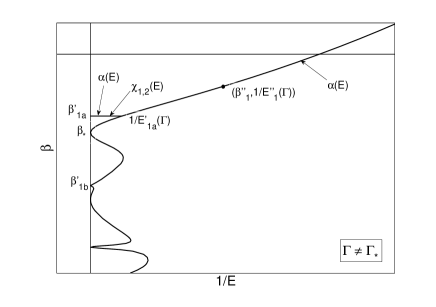
The asymptotic limit treated by Fofonoff fofonoff corresponds to small energies , a limit relevant to oceanic situations. In the statistical theory, this corresponds to a regime of large positive inverse temperatures . In that case, the Fofonoff solution is the unique (global) entropy maximum at fixed circulation and energy. On the other hand, Chavanis & Sommeria jfm studied the case of a linear relationship in a rectangular domain without topography. For large energies , corresponding to sufficiently negative , they report the existence of multiple solutions. This leads to interesting phase transitions between monopoles and dipoles depending on the value of a single control parameter and on the geometry of the domain (for example, the aspect ratio of a rectangular domain). For , the maximum entropy state is a monopole if and a dipole if . For , when the maximum entropy state is always a monopole and when , the maximum entropy state is a dipole for small values of and a monopole for large values of . The approach of Chavanis & Sommeria jfm has been completed recently by Venaille & Bouchet vb ; vbf who used a different theoretical formalism and provided a detailed discussion of phase transitions and ensemble inequivalence in QG flows with and without topography. For low values of the energy, they recover Fofonoff flows fofonoff and for large values of the energy, they obtain geometry induced phase transitions between monopoles and dipoles similar to those found by Chavanis & Sommeria jfm . They also emphasize the notions of bicritical point and azeotropy. Their approach is well-suited for statistical mechanics but it may appear a bit abstract to fluid mechanicians. By contrast, the approach of Chavanis & Sommeria jfm is simpler. In the present paper, we shall extend the formalism of jfm to the case of flows with a topography and study how the series of equilibria is modified in this more general context. We first consider an antisymmetric linear topography in a rectangular domain (like in Fofonoff’s classical study) and then generalize the results to the case of an arbitrary topography in an arbitrary domain. We recover and confirm the main results of Venaille & Bouchet vb ; vbf and illustrate them with explicit calculations and with synthetic phase diagrams. We compute the full series of equilibria (containing all the critical points of entropy at fixed energy and circulations) while Venaille & Bouchet vb ; vbf focus on global entropy maxima. The full series of equilibria is useful to show the relative position of the stable and unstable branches. Furthermore, for systems with long-range interactions, metastable states (local entropy maxima), and even saddle points of entropy, can be long-lived and therefore relevant in the dynamics ncd1 . It is therefore important to take them into account. We also give a special attention to the existence of a second order phase transition that exists only for a particular value of the circulation (with for an antisymmetric topography) and study how this phase transition takes birth as through the formation of a “spike”. Finally, we introduce simple relaxation equations that converge towards the minimum potential enstrophy state at fixed circulation and energy and solve these equations numerically to illustrate the phase transitions in a rectangular oceanic basin with linear topography (or -effect). Numerical integration of these equations with a nonlinear topography have been previously performed in cnd and the present paper develops the theory required to interpret the results.
II The quasigeostrophic equations
II.1 A maximization problem
We consider a 2D incompressible flow over a topography described by the quasigeostrophic (QG) equations
| (1) |
where is the potential vorticity, the topography, the Rossby radius, the vorticity, the stream function and the velocity field ( is a unit vector normal to the flow). For illustration and explicit calculations, we shall consider a linear topography of the form . This term can equivalently be interpreted as a “-effect” in the oceans due to the Earth’s sphericity.
The QG equations admit an infinite number of steady states of the form
| (2) |
where is an arbitrary function. They are obtained by solving the differential equation
| (3) |
with on the domain boundary. The QG equations conserve the energy
| (4) |
and an infinite number of integral constraints that are the Casimirs
| (5) |
where is an arbitrary function. In particular, all the moments of the potential vorticity are conserved. The first moment is the potential circulation and the second moment is the potential enstrophy.
Let us consider the maximization problem
| (6) |
where and are the energy and the circulation and is a functional of the form
| (7) |
where is an arbitrary convex function (i.e. ). The critical points of at fixed and are given by the variational principle where and are Lagrange multipliers. This gives . Since is convex, we can inverse this relation to obtain where . We note that . Therefore, a critical point of at fixed and determines a steady state of the QG equations with a monotonic relationship that is increasing for and decreasing for . On the other hand, this state is a (local) maximum of at fixed and iff
| (8) |
for all perturbations that conserve energy and circulation at first order.
II.2 Its different interpretations
The maximization problem (6) can be given several interpretations (see proc for a more detailed discussion):
(i) It determines a steady state of the QG equations that is nonlinearly dynamically stable according to the stability criterion of Ellis et al. eht . In that case, will be refered to as a “pseudo entropy” proc . This criterion is more refined than the well-known Arnol’d theorems arnold that provide only sufficient conditions of nonlinear dynamical stability. We note, however, that the criterion (6) provides itself just a sufficient condition of nonlinear dynamical stability. An even more refined criterion of nonlinear dynamical stability is given by the Kelvin-Arnol’d principle kelvin ; arnold2 . The connections between these different criteria of dynamical stability are reviewed in proc . For the particular choice (neg-enstrophy), the maximization problem (6) determines steady states of the QG equations with a linear relationship that are nonlinearly dynamically stable.
(ii) The maximization problem (6) can be viewed as a phenomenological selective decay principle (for ) due to viscosity mm ; proc . In the presence of a small viscosity , the fragile integrals decay (see, however, Appendix A) while the robust integrals and remain approximately conserved. This suggests that the system will reach a steady state that is a maximum of a certain functional at fixed and . If we assume that this functional is , we recover the ordinary minimum enstrophy principle introduced by Bretherton & Haidvogel bretherton (however, these authors mention in their Appendix that other functionals of the form (7), that they call generalized enstrophies, could be minimized as well). We can also justify an inviscid selective decay principle due to coarse-graining jfm ; proc . For an ideal evolution (no viscosity), the integrals of the fine-grained PV are conserved by the QG equations (they are particular Casimirs) while the integrals of the coarse-grained PV increase (see Appendix A of super ). These functionals are called generalized -functions super ; tremaine . This suggests that the system will reach a steady state that is a maximum of a certain H-function at fixed and . If we assume that this functional is , we justify an inviscid minimum enstrophy principle due to coarse-graining jfm . However, other generalized functions could be maximized as well proc . It is important to emphasize that these principles are purely phenomenological and that they are not based on rigorous arguments. As such, they are not always true brands ; proc .
(iii) The maximization problem (6) provides a necessary and sufficient condition of thermodynamical stability in the Ellis-Haven-Turkington (EHT) approach eht where the Casimir constraints (fragile) are treated canonically so that they are replaced by the specification of a prior vorticity distribution encoding small-scale turbulence. Indeed, a vorticity distribution is a maximum of relative entropy at fixed circulation and energy (EHT thermodynamical stability) iff the corresponding coarse-grained PV field is a maximum of a “generalized entropy” at fixed and eht ; aussois ; cnd . In that case, the generalized entropy is determined by the prior . For a Gaussian prior, we find that the generalized entropy is proportional to minus the macroscopic coarse-grained enstrophy, justifying a minimum potential enstrophy principle in that context.
(iv) Since the solution of a variational problem is always solution of a more constrained dual variational problem (but not the converse) ellis , the maximization problem (6) provides a sufficient condition of thermodynamical stability in the Miller-Robert-Sommeria (MRS) approach miller ; rs where all the Casimirs are conserved. Indeed, a vorticity distribution is a maximum of MRS entropy at fixed energy, circulation and Casimirs (MRS thermodynamical stability) if it is a maximum of at fixed energy and circulation. However, the converse is wrong since the Casimir constraints have been treated canonically. According to (iii), we conclude that a vorticity distribution is a maximum of MRS entropy at fixed energy, circulation and Casimirs if the corresponding coarse-grained PV field is a maximum of at fixed and (but not the converse) bouchet . In that case, the generalized entropy is determined by the initial condition proc . For initial conditions that lead to a Gaussian PV distribution at statistical equilibrium, we find that . Therefore a minimum of coarse-grained potential enstrophy at fixed circulation and energy is a MRS thermodynamical equilibrium but the converse is wrong in case of ensemble inequivalence. In the MRS approach, a minimum enstrophy principle can be justified only if the microcanonical and grand microcanonical ensembles are equivalent proc .
(v) The maximization problem (6) provides a sufficient condition of thermodynamical stability in the Naso-Chavanis-Dubrulle (NCD) approach ncd1 where only a few Casimirs are conserved (the reason is the same as in (iv)). In that case, the generalized entropy is determined by the set of conserved Casimirs. For example, if we only conserve the microscopic potential enstrophy , we find that . In that case, the generalized entropy is proportional to minus the coarse-grained enstrophy . Furthermore, in this specific case where the constraints are linear or quadratic (energy-enstrophy-circulation statistical mechanics), it can be proven that the maximization of MRS entropy at fixed energy, circulation and microscopic potential enstrophy (NCD thermodynamical stability) is equivalent to the minimization of macroscopic potential enstrophy at fixed energy and circulation ncd1 . This justifies an inviscid minimum potential enstrophy principle, and Fofonoff flows, when only the microscopic enstrophy is conserved among the infinite class of Casimirs.
II.3 Relaxation equations
Some relaxation equations associated with the maximization problem (6) have been introduced in proc . They can serve as numerical algorithms to solve this maximization problem. They also provide non trivial dynamical systems whose study is interesting in its own right.
(i) The first type of equations is of the form
| (9) |
| (10) |
where is the diffusion coefficient. The boundary conditions are where is the current and is a unit vector normal to the boundary. With these boundary conditions, the circulation is clearly conserved. On the other hand, the inverse “temperature” evolves in time according to Eq. (10) so as to conserve energy (). Easy calculations lead to the -theorem:
| (11) |
Therefore, the relaxation equations (9)-(10) relax towards a (local) maximum of at fixed and (see proc for a more precise statement).
Example: If we take to be the opposite of the potential enstrophy , we get
| (12) |
| (13) |
This equation monotonically dissipates the potential enstrophy () at fixed energy and circulation () until the minimum potential enstrophy state is reached. If we take constant and (for simplicity), the foregoing equations reduce to
| (14) |
| (15) |
where we have used an integration by parts in Eq. (13) to obtain Eq. (15). In particular, for , we have . As shown in Appendix B, these relaxation equations are compatible with the “Neptune effect” discovered by Holloway hollowaynept and playing an important role in oceanic modeling.
(ii) The second type of relaxation equations is of the form
| (16) |
where and evolve in time according to
| (17) |
| (18) |
in order to satisfy the conservation of energy and circulation ( is the domain area, and we have assumed constant for simplicity). We shall consider boundary conditions of the form on the boundary so as to be consistent with the steady state for which in the whole domain (recall that on the boundary). Easy calculations lead to the theorem:
| (19) |
Therefore, the relaxation equations (16)-(18) relax towards a (local) maximum of at fixed and (see proc for a more precise statement).
Example: If we take to be the opposite of the potential enstrophy , the relaxation equations reduce to
| (20) |
with
| (21) |
| (22) |
These equations monotonically dissipate the potential enstrophy () at fixed energy and circulation () until the minimum potential enstrophy state is reached.
III Thermodynamics of Fofonoff flows
III.1 The maximization problem
We shall study the maximization problem
| (23) |
with
| (24) |
| (25) |
| (26) |
| (27) |
For simplicity, we assume but the case of finite Rossby radius can be treated similarly and the main results are unchanged. As discussed in Sec. II.2, the maximization problem (23) can be interpreted as a refined condition of nonlinear dynamical stability (in that case is a Casimir or a pseudo entropy), as a sufficient condition of thermodynamical stability in the MRS approach, or as a necessary and sufficient condition of thermodynamical stability in the EHT and NCD approaches (in these cases is a generalized entropy). Noting that is proportional to the opposite of the potential enstrophy , the maximization problem (23) is also equivalent to the phenomenological minimum potential enstrophy principle. In the following, to simplify the terminology, will be called the “entropy”.
The critical points of entropy at fixed circulation and energy are given by the variational principle
| (28) |
where and are Lagrange multipliers that will be called “inverse temperature” and “chemical potential”. This yields
| (29) |
We consider a domain of unit area and we define . Then, we have and we can rewrite the previous relation as
| (30) |
Substituting this relation in Eq. (27), we obtain
| (31) |
with on the domain boundary. This is the fundamental differential equation of the problem. It has the form of an inhomogeneous Helmholtz equation.
III.2 The solution of the differential equation and the equation of state
To study the maximization problem (23), we shall follow the general methodology developed by Chavanis & Sommeria jfm . The main novelty with respect to their study is the presence of the topography . We shall write the topography in the form where is dimensionless.
To study the differential equation
| (35) |
we first assume that (i.e. ) and we define
| (36) |
and
| (37) |
We note that so that plays the role of the inverse of the chemical potential (see Sec. III.3). Therefore, the condition is equivalent to finite. With these notations, the differential equation (35) becomes
| (38) |
with on the domain boundary. The solution of this equation can be written
| (39) |
where and are the solutions of
| (40) |
| (41) |
with and on the domain boundary. For given , the functions and can be obtained by solving the differential equation numerically or by decomposing the solutions on the modes of the Laplacian operator (cf Appendix C). For the moment, we assume that is not equal to an eigenvalue of the Laplacian so that the solutions of Eqs. (40) and (41) are unique and finite. The cases must be studied specifically (see following sections).
Taking the average of Eq. (36) and solving for , we obtain
| (42) |
Using Eqs. (36) and (42), the solution of Eq. (35) is
| (43) |
Using Eqs. (37) and (42), the constant is given by
| (44) |
where itself depends on . Substituting Eq. (39) in Eq. (44), we finally obtain
| (45) |
For a given normalized circulation , this relation completely determines as a function of . Therefore, the solution of Eq. (35) is given by Eq. (43) where is determined by Eqs. (39) and (45). We have thus completely solved the differential equation (35) for . We must now relate to the energy. Substituting Eq. (43) in the energy constraint (32), we get
| (46) |
Similarly, the entropy (33) can be written
| (47) |
In the absence of topography (), we recover the equations of Chavanis & Sommeria jfm . In that case, there is a single control parameter . In the present case, there are two control parameters: and . In order to have a well-defined limit , it is more convenient to take and as independent control parameters. Using Eq. (44), we find that the equations of the problem are given in a very compact form by
| (48) |
| (49) |
Note that the r.h.s. of Eqs. (48) and (49) are functions of which can be easily computed numerically. There are two control parameters: the energy and the circulation (normalized by the -effect parameter or by the amplitude of the topography). For the sake of simplicity we will denote, in the figures and in the discussion, and the energy and the circulation thus normalized (while will be explicitly written in the formulae). For given , Eq. (48) determines as a function of , i.e. the caloric curve . Of course, it is easier to proceed the other way round. We first fix . Then, for each we can determine by Eq. (45) and by Eq. (48) to obtain . Inverting this relation we get for fixed .
We now consider the case (i.e. ). Equation (35) then becomes
| (50) |
and the solution is
| (51) |
Substituting this relation in Eqs. (32) and (33) and using , we find that the energy and the entropy are given by
| (52) |
| (53) |
We can check that these equations are limit cases of the general equations (48), (49) and (39) when . Indeed, the condition is equivalent to .
Particular limits: It is interesting to mention the connection with previous works. For , we recover the results of Chavanis & Sommeria jfm . This corresponds to a limit of large energies . We expect geometry induced phase transitions between monopoles and dipoles. On the other hand, for , we recover the results of Fofonoff fofonoff . This corresponds to a limit of small energies . In that case, the equilibrium state is unique and corresponds to a westward jet (in an antisymmetric domain with -effect ).
III.3 The chemical potential
The chemical potential is defined by
| (54) |
If , then
| (55) |
If , according to Eq. (37), we have
| (56) |
Therefore, up to a normalization constant, the chemical potential is equal to . This gives to the parameter a clear physical meaning.
For a given value of the energy , we can obtain the chemical potential curve in parametric form in the following manner. Fixing , we find from Eqs. (48) and (39) that is related to by a second degree equation
| (57) |
This determines . On the other hand, according to Eq. (45), the circulation is related to by
| (58) |
This determines . Therefore, for given , these equations allow us to obtain as a function of in parametric form with running parameter . This yields the chemical potential curve . Then, we have to account for the particular cases where is an eigenvalue of the Laplacian (see below).
III.4 A critical circulation
According to Eq. (45), we note that the expression of (related to the chemical potential ), involves the important function:
| (59) |
We shall call the solutions of and we shall denote simply the largest solution. The function and the inverse temperature were introduced by Chavanis & Sommeria jfm . We will see that the temperature plays an important role in the problem. For , we find that except if where is a critical circulation given by 111In fact, there exists several critical circulations , associated to each value of , but we will see that only the one corresponding to the highest inverse temperature matters when we consider stable states.:
| (60) |
We will have to distinguish the cases and .
III.5 The program
We shall successively consider the case of an antisymmetric and a non-symmetric topography. It will be shown that the mathematical expressions simplify greatly for an antisymmetric topography so that it is natural to treat this case first. To be specific, we will consider a rectangular domain and a topography of the form . This corresponds to the situation studied by Fofonoff fofonoff in his seminal paper. It should therefore be given particular attention. Then, we will consider a non-symmetric topography of the form in a rectangular domain. Finally, it will be shown in Secs. V and VI how the results can be generalized to an arbitrary domain and an arbitrary topography.
The inverse temperature is the Lagrange multiplier associated with the conservation of the energy and the chemical potential is the Lagrange multiplier associated with the conservation of the circulation . Thus, and . We shall first study the caloric curve for a given value of the circulation , then the chemical potential for a given value of the energy .
IV The case of an antisymmetric linear topography (Fofonoff case)
We consider a complete oceanic basin as in the study of Fofonoff fofonoff . The domain is rectangular with and where is the aspect ratio. The topography (i.e. ) is linear and antisymmetric with respect to . This linear topography can also represent the -effect. The eigenvalues of the Laplacian in a rectangular domain will be called (see Appendix C). Assuming , it is easy to show from considerations of symmetry that is odd and is even with respect to . Therefore,
| (61) |
When (, finite), the equations of the problem become
| (62) |
| (63) |
| (64) |
| (65) |
When (, ), the equations of the problem become
| (66) |
| (67) |
| (68) |
Finally, since , we find that . We thus need to distinguish two cases depending on whether or .
IV.1 The caloric curve for
We shall first discuss the caloric curve for . Details on the construction of this curve can be found in Appendix F.1. Since the multiple solutions occur for large values of , it appears more convenient to plot as a function of like in the study of Chavanis & Sommeria jfm . The corresponding curve can be deduced easily.
For small energies, there exists only one solution of Eq. (35) and it is a global entropy maximum at fixed circulation and energy. On the other hand, for large energies, there exists an infinite number of solutions of Eq. (35), i.e. there exists an infinite number of critical points of entropy at fixed circulation and energy. In order to select the most probable structure, we need to compare their entropies. For we have so we just need to compare their inverse temperature . More generally, it can be shown that the entropy is a monotonic function of (for given and ) so, in the following, we shall select the solution with the largest . For large energies, there is a competition between the solution with inverse temperature , the solution with inverse temperature (where is the largest eigenvalue with zero average value and ) and the solution with inverse temperature (where is the largest eigenvalue with zero average value and ). In the region where the solutions are in competition, the solution with the highest entropy is the one with . The selection depends on the aspect ratio of the domain. In a rectangular domain elongated in the horizontal direction (), . In a rectangular domain elongated in the vertical direction (), . On the other hand, as shown by Chavanis & Sommeria jfm , there exists a critical aspect ratio such that: for , for and for . To describe the phase transitions, we must therefore consider these three cases successively.

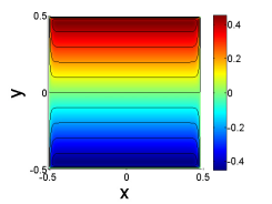
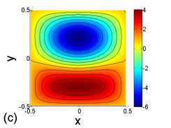
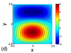
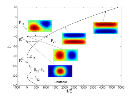
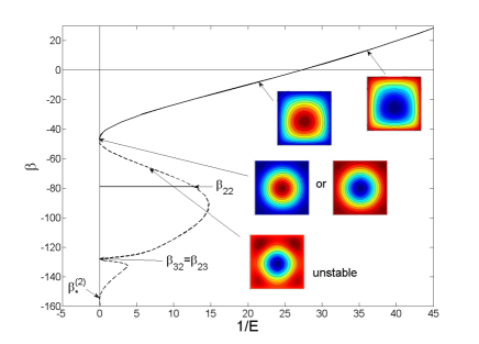
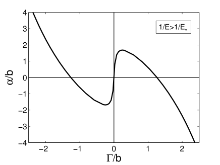
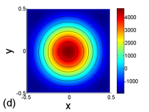
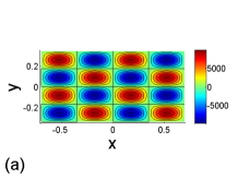
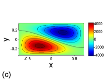
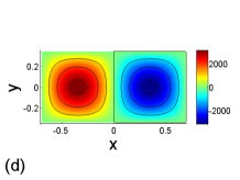
, as in Figs. 1 and 2. For small energies there exists only one solution of Eq. (35) and it is a global entropy maximum. For , leading to , we recover the classical Fofonoff solution (see Fig. 3). Far from the boundaries, the Laplacian term in Eq. (35) can be neglected, which leads to and , representing a westward jet of velocity . The eastward recirculation can be obtained from a boundary layer approximation fofonoff . For intermediate energies with , the flow involves two symmetric gyres: the gyre at has positive PV and the gyre at has negative PV. For intermediate energies and , the situation is reversed: the gyre at has negative PV and the gyre at has positive PV. All these solutions, forming the upper branch of the main curve, will be called Fofonoff flows 222For the sake of simplicity, we will call Fofonoff flows all the states with low energy. However, it is worth mentioning that the strict Fofonoff limit, corresponding to the case where is negligible with respect to , arises only for very low energies (). For a linear topography (or -effect) in an antisymmetric domain, this leads to westward jets. For intermediate energies, and the same topography, the flow consists of two gyres of opposite sign and one should rather speak of “rolls”. For other topographies, the situation is still different but, at decreasing values of the energy, the flow always tends to align with the topography.. They will be labeled (FP) and (FN) respectively. On the other hand, for large energies, there is a competition between several solutions of Eq. (35). When , the maximum entropy state is the solution with . The solution with and is a pure monopole as in the study of Chavanis & Sommeria jfm . It can rotate in either direction since the monopole (MP) with positive PV at the center and the monopole (MN) with negative PV at the center have the same entropy. For and the monopole is mixed with a Fofonoff flow. It will be called mixed monopole/Fofonoff flow. For a fixed value of , there exists two different solutions depending on the sign of (see Fig. 4). The caloric curve displays a second order phase transition marked by the discontinuity of at . In conclusion, for we have Fofonoff flows (with ), for we have mixed monopole/Fofonoff flows (with ) and for we have a pure monopole (with ).
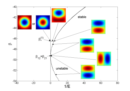
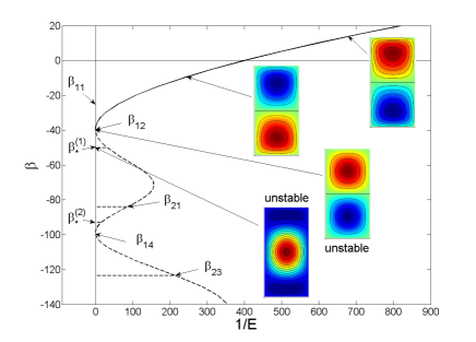
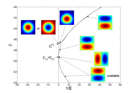
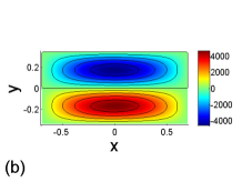
(horizontally elongated domains), as in Fig 5. For small and moderate energies, the situation is similar to that described previously (Fofonoff flows). On the other hand, for large energies, the situation is different. When , the maximum entropy state is the solution with . The solution with and is a pure horizontal dipole as in the study of Chavanis & Sommeria jfm . It can rotate in either direction since the dipole (DP) with positive PV on the left and the dipole (DN) with negative PV on the left have the same entropy. For and the dipole is mixed with a Fofonoff flow. It will be called mixed horizontal dipole/Fofonoff flow. The caloric curve displays a second order phase transition marked by the discontinuity of at . In conclusion, for we have Fofonoff flows (with ), for we have mixed horizontal dipole/Fofonoff flows (with and ) and for we have a pure horizontal dipole (with and ).
(vertically elongated domains), as in Fig. 6. For we recover Fofonoff flows as discussed previously. On the other hand, for , when , the maximum entropy state is the pure vertical dipole with . In that case, there is no phase transition: the Fofonoff flows continuously form a vertical dipole for . This can be explained by the fact that the vertical dipole does not break the symmetry of Fofonoff flows contrary to the monopoles and the horizontal dipoles in the previous cases. In conclusion, for we have Fofonoff flows (with ) and for we have a pure vertical dipole (with ).
In Fig. 7, we plot the phase diagram in the plane for . Concerning the curve at , there is a second order phase transition between Fofonoff flows and horizontal dipoles for , a second order phase transition between Fofonoff flows and monopoles for and no phase transitions for (the passage from Fofonoff flows to vertical dipoles is regular).

IV.2 The caloric curve for
We describe here the caloric curve for . Details on the construction of this curve can be found in Appendix F.2. Three cases must be considered.
, as in Figs. 8, 9 and 10. For , the maximum entropy state is an asymmetric Fofonoff flow and for , the maximum entropy state is the monopole . Since there is no plateau, the caloric curve does not display any phase transition: for , and are continuous. This is different from the case . In conclusion, for we have asymmetric Fofonoff flows (with ) and for we have a pure monopole (with ) rotating in either direction. Interestingly, when (see Fig. 10), the main curve is more and more “pinched” near the point (, . This is consistent with the formation of a plateau (second order phase transition) when .

(horizontally elongated domains), as in Figs. 11 and 12. For small energies, the maximum entropy state is an asymmetric Fofonoff flow. For , the maximum entropy state is the horizontal dipole . For intermediate energies, the maximum entropy state is a mixed horizontal dipole/asymmetric Fofonoff solution. These solutions form a plateau . In that case, the caloric curve displays a second order phase transition marked by the discontinuity of at . In conclusion, for we have asymmetric Fofonoff flows (with ), for we have mixed horizontal dipoles/asymmetric Fofonoff flows (with and ) and for we have a pure horizontal dipole (with and ) rotating in either direction.


(vertically elongated domains), as in Figs. 13 and 14. For , the maximum entropy state is an asymmetric Fofonoff flow and for , the maximum entropy state is the vertical dipole . Since there is no plateau, there is no phase transition in that case. In conclusion, for we have asymmetric Fofonoff flows (with ) and for we have a vertical dipole (with ).


In Fig. 15, we plot the phase diagram in the plane for different values of . Concerning the curve at fixed , there is a second order phase transition between Fofonoff flows and horizontal dipoles for and no phase transitions for (the passage from Fofonoff flows to monopoles and vertical dipoles is regular).
IV.3 The chemical potential curve for fixed
In the previous sections, we have studied the caloric curve for a fixed circulation . We shall now study the chemical potential curve for a fixed energy . The general equations determining the chemical potential are given by Eqs. (III.3) and (58). For an antisymmetric topography, using Eq. (61), the term in factor of in Eq. (III.3) vanishes and the foregoing equations reduce to
| (69) |
| (70) |
In that case, it is very easy to obtain the chemical potential curve for fixed , parameterized by . This curve is antisymmetric with respect to . As in Secs. IV.1 and IV.2, three cases must be considered.
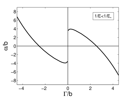
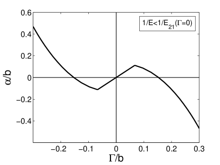
, as in Figs. 16 and 17. For and , we are on the plateau of mixed monopoles/Fofonoff flows. There exists two solutions for each energy that have two symmetric values of the chemical potential (see Fig. 4). Their values are given by Eqs. (56) and (III.3) replacing by . At the end of the plateau, for , we get . For and , we are on the main branch and the chemical potential is equal to for each energy. For there is a unique solution for each energy. In conclusion, for , the chemical potential curve displays a first order phase transition at marked by the discontinuity of . This corresponds to the transition from the monopole (MP) for to the monopole (MN) for . For , the curve is continuous and differentiable so there is no phase transition.
, as in Figs. 18 and 19. For any and , we are on the plateau of mixed horizontal dipole/Fofonoff flows. There exists two solutions for each energy (with ), but they have the same value of chemical potential . For , we are on the main branch and the chemical potential takes a unique value , corresponding to a unique solution, for each energy. For , we always have . Since is a parabola of the form with , its minimum value is obtained for . Let us now assume . Then, as long as (so that ), we are on the plateau and the chemical potential is a linear function of the circulation given by Eqs. (56) and (58) where is replaced by . For , we are on the main branch and is given by Eqs. (56), (III.3) and (58). In conclusion, if , the chemical potential curve displays two second order phase transitions between horizontal dipoles and Fofonoff flows at marked by the discontinuity of . If there is no phase transition.

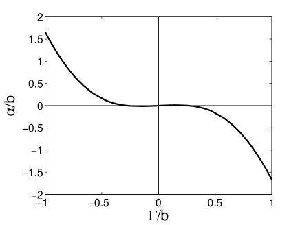
, as in Fig. 20. For any , we are on the main branch and the chemical potential takes a unique value for each energy. For , we always have . Furthermore the curve is continuous and differentiable. In conclusion, there is no phase transition.
It is interesting to mention the existence of particular points in the phase diagram. (i) For , is a critical point at which a first order phase transition appears (see Figs. 16 and 17). (ii) For energies such that , is a bicritical point: for fixed energy, the system exhibits a bifurcation from a first order phase transition (see Fig. 16) to two second order phase transitions (see Fig. 18) when increasing the aspect ratio of the domain. (iii) For , a second order azeotropy arises at , where two second order phase transitions appear simultaneously from nothing (see Fig. 18 and 19). The possible existence of these behaviors in systems with long range interactions was predicted by Bouchet & Barré bouchet_barre . It was evidenced by Venaille & Bouchet vb ; vbf for Euler and geophysical flows by extending the work of Chavanis & Sommeria jfm . We refer to these works for a more detailed description of these phase transitions. We note that the critical point and the second order azeotropy are specific to flows with topography while the bicritical point also exists when .
V The case of a non-symmetric linear topography
In the previous section, we have considered the case of a linear topography that is antisymmetric with respect to the middle axis of a rectangular domain (these results remain valid for more general antisymmetric topographies of the form ). We now consider the case of a linear topography , i.e. , with that is non-symmetric (the following results remain valid for more general non-symmetric topographies of the form ). We shall see that the details of calculations are a bit different while the structure of the main curves remains finally unchanged.
For a non-symmetric topography, there is no particular simplification of the equations of the problem. Therefore, we must use the general equations of Sec. III.2. It has been shown in Sec. III.2 that there exists a critical circulation . This critical circulation depends on the aspect ratio of the domain 333For example, for a linear topography in a semi-basin , we get . Indeed, this is equivalent to a complete basin with a topography . This is in turn equivalent to a complete basin with topography and a vorticity . The new circulation is . Since according to Sec. IV, we get . For a topography , we get . and on the form of the topography. We shall consider successively the cases and .
V.1 The caloric curve for
The series of equilibria for a non-symmetric topography when are similar to the ones obtained in Sec. IV.2 for an antisymmetric topography when (recall that in an antisymmetric domain). Details on their construction are given in Appendix F.3.
1st case: . For we have asymmetric Fofonoff flows (with ) and for we have a pure monopole (with ). The caloric curve does not display any phase transition.
2nd case: . For we have asymmetric Fofonoff flows (with ), for we have mixed horizontal dipoles/Fofonoff flows (with and ) and for we have a pure horizontal dipole (with and ). The caloric curve displays a second order phase transition at the energy .
3rd case: . For , we have asymmetric Fofonoff flows (with ) and for we have a vertical dipole (with ). There is no phase transition.
V.2 The caloric curve for
The series of equilibria in a non-symmetric domain when are similar to the ones obtained in Sec. IV.1 for an antisymmetric domain when (recall that in an antisymmetric domain). Details on their construction are given in Appendix F.4. They can also be understood from the curves of Sec. V.1 by considering the limit . When , the main curve is more and more “pinched” near the point (, and for a plateau appears at temperature between and .
If : for we have Fofonoff flows (with ), for we have mixed monopoles/Fofonoff flows (with ) and for we have a pure monopole (with ). The caloric curve displays a second order phase transition at the energy .
If : for we have Fofonoff flows (with ), for we have mixed horizontal dipoles/Fofonoff flows (with and ) and for we have a pure horizontal dipole (with and ). The caloric curve displays a second order phase transition at the energy .
If : for we have Fofonoff flows (with ) and for we have a vertical dipole (with ). There is no phase transition.
V.3 The chemical potential curve for fixed
In a non-symmetric domain, the results are similar to those obtained in Sec. IV.3 even if the general equations are a little more complicated and the curve is non-symmetric.
If : for , there is a first order phase transition at marked by the discontinuity of . For , the curve is continuous and differentiable so there is no phase transition.
If : for , there are two second order phase transitions at and marked by the discontinuity of . If , there is no phase transition.
If : there is no phase transition.
In conclusion: (i) for , is a critical point; (ii) is a bicritical point; (iii) a second order azeotropy arises for at .
VI Summary and generalizations
We shall now generalize the previous results to the case of an arbitrary domain and an arbitrary topography . Some illustrations of phase transitions in geophysical flows with different topographies are given in cnd . We here develop the theory needed to interpret them.
In the series of equilibria containing all the critical points of entropy at fixed circulation and energy, we must distinguish:
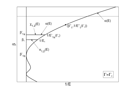
The main curve : each point of this curve corresponds to a unique solution with a unique value of the chemical potential . For (small energies), leading to , we obtain Fofonoff flows with an arbitrary topography. Far from the boundaries, we can neglect the Laplacian term in Eq. (35) leading to a stream function and a velocity field . The recirculation at the boundary can be obtained from a boundary layer approximation.
The inverse temperature : for , there is only one solution with that exists at . This is a limit point of the main curve. For , the solutions with form at plateau going from to . On this plateau, each value of the energy determines two solutions with the same temperature but with different chemical potentials and .
The inverse temperature (largest eigenvalue with ): this is a particular point of the main curve that corresponds to where is a parabola. This point marks the domain of inequivalence between the grand canonical ensemble on the one hand and the canonical and microcanonical ensembles on the other hand (see vb ; vbf and Sec. VI.3).
The inverse temperature (largest eigenvalue with and ; eigenmode with zero mean orthogonal to the topography): these solutions form a plateau going from to where is a parabola. On this plateau, each value of the energy determines two solutions with the same temperature , the same chemical potential but with different mixing coefficients and .
The inverse temperature (largest eigenvalue with and ; eigenmode with zero mean non orthogonal to the topography): it exists only at . This is a limit point of the main curve.
The series of equilibria showing these different solutions is represented schematically in Fig. 21 for and in Fig. 22 for . In the domain of competition, where there exists several solutions for the same energy, we must select the solution with the largest , which is the maximum entropy state. Thus, in this range, . Note that the value of only depends on the geometry of the domain and on the form of the topography.
VI.1 The caloric curve
Let us first describe the caloric curve for a given value of . We need to distinguish three cases:
1. If : (i) If , we have a second order phase transition since is discontinuous at . (ii) If , there is no phase transition.
2. If : we have a second order phase transition since is discontinuous at . This is because is orthogonal to the topography leading to a symmetry breaking. However, this situation is not generic (see the remark at the end of VI.2).
3. If : there is no phase transition. This is because is not orthogonal to the topography, so that there is no symmetry breaking.
VI.2 The chemical potential curve
Let us now describe the chemical potential curve for a given value of . We need to distinguish three cases:
1. If : if , there is a first order phase transition at since is discontinuous at . For , there is no phase transition.
2. If : if , there are two second order phase transitions at and . For , there is no phase transition.
3. If : there is no phase transition.
All these results are fully consistent with those obtained by Venaille & Bouchet vb ; vbf using a different theoretical treatment.
Remark: in general, the topography (e.g. in the oceans) is very complex and is generically not orthogonal to an eigenmode of the Laplacian, so that does not exist (note also that zero mean eigenmodes exist only if the domain has specific symmetries which is generally not the case in the oceans). In addition, in generic situations, . Therefore, in typical caloric curves , there are no plateaus at and (see, e.g., cnd ). Consequently, the interesting phase transitions (second order, bicritical points, azeotropy,…) described in vb ; vbf and in this paper do not generically exist in geophysical flows (with complex topographies). One notorious exception of physical interest is the case of a rectangular basin with a linear topography (treated explicitly in Secs. IV and V) corresponding to the -effect, or the case of topographies of the form or . However, for more complex topographies there is no phase transition in the strict sense. Nevertheless, there always exists at least a “smooth” transition from a monopole to a dipole when we stretch the domain (at fixed high energy), and a “smooth” transition from a monopole or a dipole to a Fofonoff flow when we lower the energy (at fixed domain shape). On the other hand, is always at least a critical point at which a first order phase transition appears (for sufficiently high energies).
VI.3 Thermodynamical stability
In the previous sections, when several solutions were in competition for the same values of and , we have compared their entropies to select the maximum entropy state. It turns out that the maximum entropy state is the solution with the highest inverse temperature jfm . Therefore, if we consider fully stable states (global entropy maxima at fixed energy and circulation), the strict caloric curve corresponds to . We can also study the thermodynamical stability of the solutions by determining whether they are (local) entropy maxima or saddle points of entropy. Complementary stability results have been obtained by Chavanis & Sommeria jfm , Venaille & Bouchet vb ; vbf and Naso et al. ncd1 . We shall briefly recall their results and refer to the corresponding papers for more details.
Chavanis & Sommeria jfm and Naso et al. ncd1 have obtained sufficient conditions of microcanonical instability by considering the effect of “dangerous” perturbations on the equilibrium states. Using their methods, it can be shown that the solutions with are unstable in the microcanonical ensemble. On the other hand, when , it can be shown that the solution corresponding to and is unstable in the microcanonical ensemble. By continuity, all the plateau should be unstable (since the two extremities of this plateau are unstable).
Venaille & Bouchet vb ; vbf have shown that the solutions with are stable in the canonical ensemble (hence in the microcanonical ensemble) while the other solutions are unstable in the canonical ensemble. However, as discussed by Chavanis & Sommeria jfm and Naso et al. ncd1 , some of these solutions can be metastable (local entropy maxima) in the microcanonical ensemble.
For , the solutions are stable in the grand canonical ensemble (hence in the canonical and microcanonical ensembles) vb ; vbf . This is related to the Arnold theorem (see, e.g., proc ). For , the solutions are stable in the canonical (hence microcanonical) ensemble but not in the grand microcanonical ensemble. This corresponds to a situation of ensemble inequivalence vb ; vbf .
VII Numerical simulations
We shall now perform numerical simulations to illustrate the phase transitions described in the previous sections. To that purpose, we use the relaxation equations of Sec. II.3 that can serve as numerical algorithms to compute maximum entropy states with relevant constraints. We shall first integrate numerically Eq. (20), with the constraints (21,22), in an antisymmetric square domain with a linear topography and two different initial conditions such that . We use as boundary conditions:
| (71) | |||
| (72) |
where is the domain boundary. The first condition enforces free-slip on the boundary, while the second one is necessary for consistency of the steady state, characterized by Eq. (29).
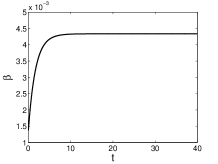
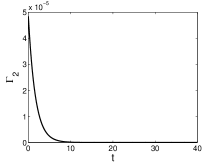
We first integrate the relaxation equations with an initial condition, , written as the sum of sine functions with random amplitudes and wave numbers ranging from 1 to 9 (see Fig. 23(a)). With such a field, and the energy is rather low: . The coefficient is set to . The resulting density of potential vorticity at different times is plotted in Fig. 23. As expected with such a low value of the energy (see Fig. 1), the relaxation equation converges to a Fofonoff state. The inverse temperature and the enstrophy are plotted as a function of time in Fig. 24. As expected, monotonically decreases in time (equivalently, the entropy increases). On the other hand, the inverse temperature monotonically increases during the simulation. Both quantities remain constant once the steady state (Fofonoff flow, maximum of entropy) has been reached.

These results can be compared with those of Wang & Vallis wang . In this study, the authors integrate the quasigeostrophic equation with linear topography in an antisymmetric square domain, with initial conditions (random eddies) and boundary conditions (free-slip) similar to ours. After about 10 eddy turnover times, the time averaged flow converges to a state close to the Fofonoff solution. Comparing our Fig. 23 with Fig. 4 of wang , it is clear that the dynamical behavior of the coarse-grained potential vorticity solution of the relaxation equation is reminiscent of that of the time averaged solution of the quasigeostrophic equation. In both cases, the eddies are first pushed to the western boundary, then two gyres form. These structures grow and fill out the northern and southern parts of the domain. Therefore, even if the relaxation equations are not supposed to provide a realistic parametrization of 2D turbulence, they may however give an idea of the true evolution of the flow towards statistical equilibrium. It is worth noticing that, with the relaxation equations, the steady state has been reached after about time steps, while it took more than several ten thousands time steps for the quasigeostrophic equation to reach the statistically steady state. Indeed, by construction, the relaxation equations “push” the system in the direction of the statistical equilibrium state.
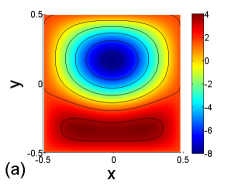
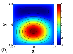
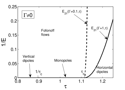
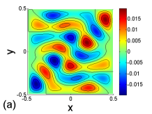
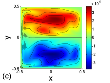
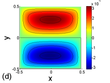
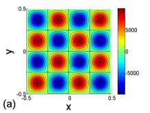
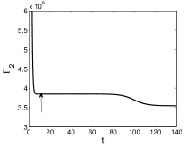
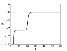
We then impose an initial condition of high energy, (see Fig. 25(a)) and integrate numerically Eq. (20), with the constraints (21,22). Since we are only interested in the final state, and not in the way the system converges towards it, we do not implement the advection term. The coefficient is set to . The density is plotted at different times in Fig. 25, and the time evolutions of the inverse temperature and of the enstrophy are shown in Fig. 26. We find that the system first relaxes spontaneously towards a horizontal dipole (see Fig. 25(b) and first plateaus of Fig. 26). In the absence of external perturbation, the system remains in this state for a long time, even if it is predicted to be unstable (see Fig. 2). It can be noticed that the value of the inverse temperature is slightly smaller than , confirming that the system is on the lower branch of Fig. 2. As already shown in the case of the 2D Euler equations ncd1 , we illustrate here that saddle points can be very long-lived. Inspired by the stability analysis performed in ncd1 , we add to the system, at , a perturbation of the form , where is the solution of Eq. (40) for (see ncd1 ). As expected (see Fig. 2), the system is then immediately destabilized, and relaxes towards the monopole which is the maximum entropy state (Fig. 25(c-d) and second plateau of Fig. 26). Depending on the sign of the perturbation, the system can relax towards the direct or towards the inverse monopole.

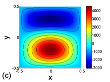

To summarize, we have illustrated the fact that in an antisymmetric square domain with linear topography, if , the stable state is strongly correlated to the topography at low energy (Figs. 23 and 24), but is not influenced by it at high energy (Figs. 25 and 26). At high energy, it is influenced by the domain geometry: in a square domain, we get a monopole whereas in a rectangle sufficiently elongated in the direction (), we get a dipole. To illustrate this remark, we integrate numerically Eq. (20), with the constraints (21,22), in an antisymmetric rectangular domain of aspect ratio , starting from an initial condition of zero circulation and of high energy (). The resulting potential vorticity density is plotted at different times in Fig. 27. The system first converges towards the vertical dipole (saddle point), with (see Fig. 27(b) and first plateaus of Fig. 28). It then destabilizes spontaneously, and converges towards the horizontal dipole (stable state) (see Fig. 27(d) and second plateaus of Fig. 28), with . These results can be compared to Fig. 5.

Other numerical simulations of the relaxation equations illustrating phase transitions in geophysical flows with nonlinear topography are reported in cnd . Interestingly, the initial conditions of high energy that we have considered in the present paper are similar to those used in Fig. 7(c) (square domain) and 8 (rectangular domain of aspect ratio ) of cnd : is proportional to and the energies are identical. We find that the final states are the same with both topographies. This is to be expected since the topography should not influence the maximum entropy state in the limit of high energy. However, we observe that the relaxation equations with the nonlinear topography of cnd directly converge towards the equilibrium state whereas, with the linear topography, the system first converges towards the vertical dipole (saddle point). Therefore, at very high energy, while the topography does not influence the stable states, it seems to play a role in the dynamics of the relaxation. Of course, this conclusion is reached on the basis of our relaxation equations. It would be interesting to know whether it remains valid for more realistic parameterizations.
VIII Conclusion
In this paper, we have studied the nature of phase transitions in simple models of oceanic circulation described by the QG equations with an arbitrary topography . We have assumed a linear relationship between potential vorticity and stream function corresponding to minimum potential enstrophy states. We have given several interpretations of this minimum potential enstrophy principle in connection with statistical mechanics, phenomenological selective decay principles, and nonlinear dynamical stability. We have explicitly treated the case of a rectangular basin and an antisymmetric linear topography like in Fofonoff’s classical paper. For small energies, we recover Fofonoff’s westward jet solution. In that case, the flow is strongly influenced by the topography and only weakly by the domain geometry. For large energies, we obtain geometry induced phase transitions between monopoles and dipoles like in the study of Chavanis & Sommeria jfm . In that case, the flow is strongly influenced by the domain geometry and only weakly by the topography. In rectangular domains elongated in the direction (), as we decrease the energy of the flow, we describe symmetry breaking phase transitions between horizontal dipoles and Fofonoff flows. Alternatively, in rectangular domains elongated in the direction (), the smooth transitions between vertical dipoles and Fofonoff flows occur without symmetry breaking. This phenomenology, illustrated in a rectangular domain with a linear topography, has been generalized to arbitrary domains and arbitrary topography.
Our study returns and confirms the results previously obtained by Venaille & Bouchet vb ; vbf by a different method. These authors provide a very detailed statistical analysis of the problem, emphasizing the notions of bicritical points, azeotropy and ensemble inequivalence. Our approach, that is less abstract and illustrated by several explicit calculations, provides a useful complement to their study. It gives another way of describing the complicated and rich bifurcations that occur in geophysical flows. Our theoretical results extend the work of Chavanis & Sommeria jfm to the case of geophysical flows (with a topography) and allow to interpret the phase transitions studied numerically by Chavanis et al. cnd in the case of complex topographies.
Appendix A Minimum potential enstrophy principle
We shall here discuss the difficulty to justify a minimum potential enstrophy principle based on the viscosity. In the presence of viscosity, the QG equations become
| (73) |
where . We emphasize that the quantity dissipated by viscosity is the vorticity , not the potential vorticity . Therefore, the rate of change of potential enstrophy is
| (74) |
For the 2D Navier-Stokes equation (), we obtain after an integration by parts
| (75) |
so that the enstrophy decreases monotonically under the effect of viscosity. However, for the viscous QG equations, we do not have a monotonic decay of potential enstrophy. Following Bretherton & Haidvogel bretherton , we must assume in Eq. (74) in order to have a monotonic decay of potential enstrophy. In more general cases, the phenomenological minimum potential enstrophy principle is not clearly justified. These remarks also apply to the functionals (7). Indeed, while these functionals increase monotonically under the effect of viscosity for the 2D Navier-Stokes equations since , their monotonic increase is not guaranted for the QG equations unless .
Therefore it is difficult to justify a principle of the form (6) for the viscous QG equations. By contrast, the interpretations of this principle that we have given in the framework of the inviscid QG equations are valid.
Appendix B Link with the Neptune effect
In this Appendix, we show that the relaxation equations of Sec. II.3 are consistent with the Neptune effect of Holloway hollowaynept . This discussion is related to the one given by Kazantsev et al. kazantsev but the justification of the relaxation equations that we consider is different.
Let us first consider the case and and derive the relaxation equation for the velocity field. We start from the equation for the vorticity field (9) that becomes
| (76) |
where we recall that can depend on position and time. For a 2D field, we have the identity . Therefore, we can rewrite the foregoing equation as
The corresponding equation for the velocity field is
where is the pressure and the density. To pass from Eq. (B) to Eq. (B), we have used the identity and the identity that is valid for a 2D incompressible flow, so that finally . Now, using and the identity
| (79) |
valid for a 2D incompressible flow, we finally obtain
We see that the drift term in the equation for the vorticity takes the form of a friction in the equation for the velocity. Furthermore, the friction coefficient is given by an Einstein-type formula involving the diffusion coefficient and the inverse temperature. At equilibrium,
| (81) |
This equation can be directly derived from the relation determining the steady states of Eq. (76). Combining , and , we recover Eq. (81). In particular, if is the opposite of the enstrophy , the relaxation equation (B) becomes
| (82) |
At equilibrium, .
Let us now consider the relaxation equation (9) including a topography . It can be rewritten
| (83) |
Proceeding as before, the corresponding equation for the velocity field is
| (84) | |||||
where we have used for a 2D incompressible velocity field. In particular, if is the opposite of the potential enstrophy , the relaxation equations (83) and (84) become
| (85) |
and
| (86) | |||||
Inspired by the original idea of Holloway hollowaynept , we introduce a velocity field based on the topography
| (87) |
With these notations, the equation for the velocity field can be rewritten
| (88) | |||||
It involves a turbulent viscosity and a friction force proportional to the difference between the velocity field and the velocity field based on the topography. The friction coefficient is given by an Einstein relation . This term “pushes” the flow towards the topographic flow . This corresponds to the so-called “Neptune effect” of Holloway hollowaynept . On the other hand, the diffusion term allows some deviation with respect to the topographic flow. At equilibrium
| (89) |
If is constant, the equation (85) for the vorticity can be written
| (90) |
At equilibrium,
| (91) |
If we neglect the Laplacian, we get . This is valid in the limit . This is equivalent to neglecting the Laplacian in the fundamental differential equation . This leads to , equivalent to and . As we have seen, this corresponds to the standard Fofonoff fofonoff flows that are completely determined by the topography (far from the boundaries). More generally, Eq. (91) takes into account finite temperature effects that can induce deviations to the standard Fofonoff flows. These finite temperature effects (corresponding to sufficiently high energies) are precisely those that have been described in this paper.
In conclusion, the relaxation equation (9) derived from the Maximum Entropy Production Principle (MEPP) proc is relatively consistent with the oceanographic parametrization of Holloway hollowaynept , especially when the (generalized) entropy is the neg-enstrophy. This is interesting because the parametrization of Holloway hollowaynept has been used in realistic oceanic modeling where the Neptune effect was shown to play a significant role. This suggests that our parametrization can be of relevance also in the physics of the oceans.
Appendix C Modal decomposition
We define the eigenfunctions and eigenvalues of the Laplacian by
| (92) |
with on the domain boundary. These eigenfunctions are orthogonal and normalized such that . Since , we note that . Following Chavanis & Sommeria jfm , we distinguish two types of eigenmodes: the odd eigenmodes such that and the even eigenmodes such that . We note and the corresponding eigenvalues.
In a rectangular domain of unit area whose sides are denoted and (where is the aspect ratio), the eigenmodes and eigenvalues are
| (93) |
| (94) |
where the origin of the Cartesian frame is taken at the center of the domain. The integer gives the number of vortices along the -axis and the number of vortices along the -axis. We have if or is even and if and are odd. The largest eigenvalue with non zero mean is . The largest eigenvalue with zero mean is for and for .
We want to solve the differential equations
| (95) |
and
| (96) |
with and on the domain boundary. This can be done by decomposing the solutions on the eigenmodes of the Laplacian using .
For , the solution of Eq. (95) is unique and given by
| (97) |
From this relation, we obtain
| (98) |
| (99) |
| (100) |
For , the solution of Eq. (96) is unique and given by
| (101) |
From this relation, we obtain
| (102) |
| (103) |
| (104) |
We also have
| (105) |
Finally, we remark that
| (106) |
On the other hand, if the topography is antisymmetric with respect to (as in the case of a linear topography ), we have implying
| (107) |
In that case, is even and is odd with respect to the variable . This can be directly seen at the level of the differential equations (95) and (96).
Appendix D The case
It can be interesting to consider the case specifically. This regime of infinite temperatures corresponds to uniform potential vorticity . The differential equation (35) reduces to
| (108) |
The solution is where and are the solutions of Eqs. (40) and (41) with . The equation for the energy (48) can be written
| (109) |
where we have used according to Eq. (45). For given , Eq. (109) determines the energy for which (i.e. is uniform). It is given by a parabola. If the topography is antisymmetric with respect to , using Eq. (107), the foregoing equation reduces to
| (110) |
Appendix E The low energy limit
In the limit , a boundary layer approximation can be made. As a first approximation, the Laplacian can be neglected in the differential equations (40) and (41), everywhere in the domain except close to the boundary. To leading order, the function is given by . The correction, close to the boundary, behaves like , where is a coordinate perpendicular to the boundary pointing towards the inside of the domain. The constant is determined by the condition on the boundary. Similarly, to leading order, the function is given by with a correction scaling like close to the boundary.
In this limit, we obtain
| (111) |
| (112) |
Similarly,
| (113) |
| (114) |
Finally, substituting these results in the energy equation (64), we obtain for :
Appendix F Technical construction of the caloric curves
F.1 Antisymmetric linear topography and
Several cases must be considered in order to construct the caloric curve. In the first one, and (i.e. , ). Since with , these solutions exist for any value of . The curve relating their temperature to the energy is given by Eq. (67). This forms the main curve (see Figs. 1, 2, 5 and 6). The entropy of these solutions is given by Eq. (68).
Another possible situation is and (i.e. , finite). According to Eq. (63), we see that is finite iff , i.e. . Therefore, the temperatures of these solutions take only discrete values. The value of is determined by the energy according to Eq. (64) with replaced by . This determines two solutions (i.e ) for each value of the energy (see for instance Fig. 4). The ensemble of these solutions form a plateau (see Figs. 1, 2, 5 and 6) starting at (, ) and connecting the main curve at (, ). When , we find . On the other hand, is given by Eq. (67) with replaced by . The evolution of with is shown in Fig. 7.
Finally, it will be assumed that is equal to an eigenvalue of the Laplacian. In that case, is necessarily equal to (i.e. , ), which corresponds to . Four cases must be distinguished:
Case 1: with and . This is not possible for an antisymmetric topography.
Case 2: with and ( odd and even) like . In that case, Eq. (41) has no solution for and diverges like
| (116) |
for . Then, we find from Eqs. (67) and (68) that and . This is a limit case of the main curve. Note that the sign of (hence ) changes as we pass from to .
Case 3: with and ( even and arbitrary) like . In that case, the solution of Eq. (41) with is not unique. To the solution (102) of Eq. (41) with we can always superpose the eigenmode with an amplitude . This corresponds to a “mixed solution”
| (117) |
which has zero average as required. The amplitude is determined by the energy constraint (67) with replaced by . This determines two solutions for each value of the energy (note that these two distinct solutions have the same value of the chemical potential ). The ensemble of these mixed solutions form a plateau (see Figs. 1, 2, 5 and 6) starting from () and connecting the main curve at (). For , we find . On the other hand, is given by Eq. (67) with replaced by . The evolution of with is shown in Fig. 7. Note that in a square domain (), since by symmetry, we find that for even and odd according to Case 2 (see Figs. 1 and 2). In that case, the plateau reduces to a point.
Case 4: with and ( odd and odd) like . In that case, the solution of Eq. (41) with is not unique and we expect a mixed solution of the form . However, has a zero average value (as required) only for . Hence, we are just left with a limit case of the main curve. It corresponds to the energy given by Eq. (67) with replaced by .
F.2 Antisymmetric linear topography and
Once more, several cases must be considered. It can be first assumed that and (i.e. , ), which corresponds to . Since , there are no such solutions for and .
Another possibility is and (i.e. , finite). These solutions exist for any value of . The curve relating their temperature to their energy is given by Eqs. (63) and (64). This forms the main curve (see Figs. 8-14). Their entropy is given by Eq. (65). For , we have leading to . In that case, . The caloric curve is unchanged when since only appears in the equation for the energy. However, the sign of (hence of ) changes when so that the flow structure is different. In the figures, we consider .
Finally, if is equal to an eigenvalue of the Laplacian, four cases must be distinguished.
Case 1: with and . This is not possible for an antisymmetric topography.
Case 2: with and ( odd and even) like . We are necessarily in the case (i.e. , finite). We see that Eq. (41) has no solution for and that diverges like
| (118) |
when . In that case and . This is just a limit case of the main curve. Note that the sign of (hence ) changes as we pass from to .
Case 3: with and ( even and arbitrary) like . We are necessarily in the case (i.e. , finite). The solutions of Eqs. (40) and (41) are not unique since we can always superpose to Eqs. (97) and (101) an eigenfunction of the Laplacian. Thus
| (119) |
| (120) |
The amplitude is determined by the energy constraint (64) with replacing . This determines two solutions for each value of (note that these two distinct solutions have the same value of , hence of , given by Eq. (63)). The ensemble of these mixed solutions form a plateau (see Figs. 8-14) starting from () and reaching the main curve at (). For , we find . On the other hand, is given by Eqs. (63) and (64) replacing by . It corresponds to a parabola of the form with (since jfm ). The evolution of with is shown in Fig. 15 for different values of . Note that in a square domain (), since by symmetry, we find that for even and odd according to Case 2 (see Figs. 8-10). In that case, the plateau is reduced to a point.
Case 4: with and ( odd and odd) like . If we consider (i.e. , finite), we see that Eq. (40) has no solution for and that diverges like
| (121) |
for . Then we find that and that tends to a finite value
| (122) |
with . It corresponds to a parabola of the form . This is just a limit case of the main curve. If we consider (i.e. , infinite) so that , we see that the solution of Eq. (41) is not unique for since we can always superpose to Eq. (101) an eigenfunction of the Laplacian. Thus
| (123) |
The condition , reducing to , determines the value of . Then, using Eq. (67), we find that this solution exists for a unique value of the energy given by Eq. (122). This is to be expected since when . In conclusion, the case or with and odd is just a limit case of the main curve.
F.3 Non-symmetric linear topography and
The first case that will be treated is the one for which and (i.e. , finite). These solutions exist for any value of . The curve relating their temperature to their energy is given by Eqs. (48), (39) and (45). This forms the main curve. Their entropy is given by Eq. (49). For we have leading to . In that case, .
Another possibility is and (i.e. , ). In that case which implies . Therefore, this solution exists for a very particular value of the inverse temperature that will be denoted . The corresponding energy is given by Eq. (52) where is replaced by . It turns out that this is just a particular point of the main branch corresponding to so that it does not bring any new solution.
In the case where is equal to an eigenvalue of the Laplacian, four cases must be distinguished.
Case 1: with and ( odd and odd) like . In that case, Eqs. (40) and (41) do not have any solution for and the functions and behave like
| (124) |
| (125) |
when . We are in the case (i.e. , finite). Substituting the asymptotic expansions (124) and (125) in Eqs. (39) and (45), we find that
| (126) | |||||
and
| (127) |
Therefore and are finite as . Substituting these results in Eq. (48), we obtain a finite energy
| (128) |
This solution is a particular case of the main curve. We note that the energy (128) is of the form with so that it forms a parabola. The minimum value of this parabola is reached for with
| (129) |
Case 2: with and ( odd and even) like . In that case, Eq. (41) does not have any solution for and diverges like
| (130) |
when . We note that . Therefore, if , we are in the case (i.e. ). Then, is finite and so that according to Eq. (48). If , we are in the case (i.e. ). Then, according to Eq. (52). This is a limit case of the main curve.
Case 3: with and ( even and arbitrary) like . The solutions of Eqs. (40) and (41) are not unique since we can always superpose to Eqs. (97) and (101) an eigenfunction of the Laplacian. Thus
| (131) |
| (132) |
The amplitude is determined by the energy constraint (48), replacing by and introducing Eqs. (131) and (132). This determines two types of solutions and for each value of the energy (note that these two distinct solutions have the same value of , hence the same value of , given by Eq. (45)). The ensemble of these mixed solutions form a plateau starting from () and reaching the main curve at (). For , we find . On the other hand, is given by Eqs. (48), (39) and (45) replacing by and taking . It corresponds to a parabola of the form with . We shall denote by the minimum value of this parabola reached for . The expressions of these quantities can easily be obtained from Eqs. (48), (39) and (45) but they are not particularly simple so we shall not give them explicitly. Note that in a square domain (), since by symmetry, we find that for even and odd according to Case 2. In that case, the plateau reduces to a point.
Case 4: with and . This is not possible for a topography of the form with .
F.4 Non-symmetric linear topography and
It will be first assumed that and (i.e. , finite). These solutions exist for any value of . For , the curve relating their temperature to their energy is given by Eqs. (48), (39) and (45). This forms the main curve. Their entropy is given by Eq. (49). For , the situation is different because Eq. (45) takes in indeterminate form. In that case, is determined by the energy constraint (48) with replaced by . This yields two solutions and (and, correspondingly, two values of the chemical potential and ) for each value of the energy. The ensemble of these solutions form a plateau starting from (, ) and reaching the main curve at (, ). When , we find . On the other hand, is given by Eq. (52) with replaced by .
A second possibility is and (i.e. , ). In that case , which implies . These solutions exist for such that . Except in an antisymmetric domain where they exist for any (see Sec. IV.1), in a non-symmetric domain they exist only for and for the corresponding value of the energy . This is just a particular point of the main curve corresponding to so this case does not bring any new solution.
The study of the eigenvalues leads to the
same results as in the previous section.
Appendix G Interest of the relaxation equations
Relaxation equations for two-dimensional flows have been introduced by Robert & Sommeria rsmepp in the context of the MRS statistical theory and extended by Chavanis proc to more general situations. These relaxation equations are relatively ad hoc since they are solely based on general “principles” similar to the first and second principles of thermodynamics: conservation of energy (and possibly other constraints) and increase of an “entropic” functional. Contrary to the Boltzmann equation, the relaxation equations are not derived from first principles but just assumed444An attempt to derive these relaxation equations from a quasilinear theory of the 2D Euler equation is made in quasi .. This is the reason why they exist in different forms. There is no general consensus about the importance and interest of these relaxation equations. Some researchers argue that they are useless and that they have no physical relevance. Other workers, on the other hand, consider that they are interesting for the following reasons:
(i) They can be used as numerical algorithms to solve maximization problems of the form (6) with a general “entropic functional” of the form (7). This maximization problem can have various interpretations (as explained in Section II.2 and in proc ) related to thermodynamical and/or nonlinear dynamical stability of 2D Euler flows. Although the case of a quadratic functional (24) can be treated analytically (as done in our paper), the general maximization problem (6)-(7) is more complex and the relaxation equations can be a way (among others) to solve it. Indeed, it is generally difficult to directly solve the Euler-Lagrange equations associated with (6)-(7) and be sure that the critical points are entropy maxima. By contrast, the relaxation equations guarantee (by construction) that the relaxed state is an entropy maximum with appropriate constraints. Furthermore, when several entropy maxima (metastable states) exist for the same values of the constraints, the relaxation equations can tell which (local) maximum will be reached by a given initial condition, thus unveiling its basin of attraction. Finally, by introducing in the relaxation equations a variable diffusion coefficient (related to the local fluctuations of vorticity), we can take into account the important effects of incomplete relaxation and lack of ergodicity rr ; csr . This is not possible if we consider just equilibrium statistical mechanics.
(ii) They provide non trivial dynamical systems, consistent with the equilibrium states, whose mathematical study is interesting in its own right. For example, we have observed that the system can remain blocked for a long time in an unstable state before finally reaching the maximum entropy state. Although this effect might be an artefact of the relaxation equations, the same phenomenon could also occur in more realistic parametrizations. Therefore, the study of the relaxation equations can suggest interesting ideas and developments.
(iii) The discussion of Appendix B shows that the relaxation equations are remarkably consistent with the parametrization of Holloway hollowaynept based on relatively different arguments. This is a hint that our parametrization may contain ingredients that capture some features of real oceanic circulation. For example, Holloway has shown that the Neptune effect plays some role in the dynamics of the oceans. Therefore, making contact between the two approaches is of interest. Furthermore, it is possible to include other geophysical effects in the relaxation equations such as wind forcing like in Kazantsev et al. kazantsev .
References
- (1) G. Holloway, Annu. Rev. Fluid Mech. 18, 91 (1986)
- (2) H. Stommel, Trans. Amer. geophys. Un. 29, 202 (1948)
- (3) W.H. Munk, J. Meteorol. 7, 79 (1950)
- (4) N.P. Fofonoff, J. Mar. Res. 13, 254 (1954)
- (5) J. Pedlosky, Geophysical Fluid Dynamics (Springer, Berlin, 1897)
- (6) G. Veronis, Deep-Sea Res. 13, 31 (1966)
- (7) A. Griffa, R. Salmon, J. Mar. Res. 49, 53 (1989)
- (8) P.F. Cummins, J. Mar. Res. 50, 545 (1992)
- (9) J. Wang, G.K. Vallis, J. Mar. Res. 52, 83 (1994)
- (10) E. Kazantsev, J. Sommeria, J. Verron, J. Phys. Oceano. 28, 1017 (1998)
- (11) P.P. Niiler, Deep-Sea Res. 13, 597 (1966)
- (12) J. Marshall, G. Nurser, J. Phys. Oceano. 16, 1799 (1986)
- (13) F.P. Bretherton, D.B. Haidvogel, J. Fluid. Mech. 78, 129 (1976)
- (14) R. Kraichnan, J. Fluid. Mech. 67, 155 (1975)
- (15) R. Salmon, G. Holloway, M.C. Hendershott, J. Fluid. Mech. 75, 691 (1976)
- (16) J. Miller, Phys. Rev. Lett. 65, 2137 (1990)
- (17) R. Robert, J. Sommeria, J. Fluid. Mech. 229, 291 (1991)
- (18) R. Ellis, K. Haven, B. Turkington, Nonlin. 15, 239 (2002)
- (19) P.H. Chavanis, Physica D 200, 257 (2005)
- (20) P.H. Chavanis, Physica D 237, 1998 (2008)
- (21) A. Naso, P.H. Chavanis, B. Dubrulle, Eur. Phys. J. B 77, 187 (2010)
- (22) P.H. Chavanis, J. Sommeria, J. Fluid. Mech. 314, 267 (1996)
- (23) A. Venaille, F. Bouchet, Phys. Rev. Lett. 102, 104501 (2009)
- (24) A. Venaille, F. Bouchet, submitted to J. Stat. Phys.
- (25) P.H. Chavanis, A. Naso, B. Dubrulle, Eur. Phys. J. B 77, 167 (2010)
- (26) P.H. Chavanis, Eur. Phys. J. B 70, 73 (2009).
- (27) V.I. Arnol’d, J. Méc. 5, 29 (1966)
- (28) L. Kelvin, Phil. Mag. 23, 529 (1887)
- (29) V.I. Arnol’d, Izv. Vyssh. Ucheb. Zaved. Matem 54, 3 (1966)
- (30) W. Matthaeus, D. Montgomery, Ann. N.Y. Acad. Sci. 357, 203 (1980)
- (31) P.H. Chavanis, Physica A, 359, 177 (2006)
- (32) S. Tremaine, M. Hénon, D. Lynden-Bell, MNRAS 219, 285 (1986)
- (33) H. Brands, P.H. Chavanis, R. Pasmanter, J. Sommeria, Phys. Fluids 11, 3465 (1999)
- (34) R. Ellis, K. Haven, B. Turkington, J. Stat. Phys. 101, 999 (2000)
- (35) F. Bouchet, Physica D 237, 1978 (2008)
- (36) G. Holloway, J. Phys. Oceano. 22, 1033 (1992)
- (37) F. Bouchet, J.Barré, J. Stat. Phys. 118, 1073 (2005)
- (38) R. Robert, J. Sommeria, Phys. Rev. Lett. 69, 2776 (1992)
- (39) P.H. Chavanis, Phys. Rev. Lett. 84, 5512 (2000)
- (40) R. Robert, C. Rosier, J. Stat. Phys. 86, 481 (1997)
- (41) P.H. Chavanis, J. Sommeria, R. Robert, Astrophys. J. 471, 385 (1996)