Soliton Trap in Strained Graphene Nanoribbons

Abstract

The wavefunction of a massless fermion consists of two chiralities, left-handed and right-handed, which are eigenstates of the chiral operator. The theory of weak interactions of elementally particle physics is not symmetric about the two chiralities, and such a symmetry breaking theory is referred to as a chiral gauge theory. The chiral gauge theory can be applied to the massless Dirac particles of graphene. In this paper we show within the framework of the chiral gauge theory for graphene that a topological soliton exists near the boundary of a graphene nanoribbon in the presence of a strain. This soliton is a zero-energy state connecting two chiralities and is an elementally excitation transporting a pseudospin. The soliton should be observable by means of a scanning tunneling microscopy experiment.

For a massless fermion, the left-handed and right-handed chiralities are a good quantum number and the two chirality eigenstates evolve independently according to the Weyl equations. One chirality state goes into the other chirality state under a change in parity. The weak interactions in elementary particle physics act differently on the left-handed and right-handed states, which results in well-known phenomena, such as the parity violation for nuclear $\beta$ decay. Sakurai (1967) The weak force is described by a gauge field. In general, a gauge field which has a different (the same) sign of the coupling for the left-handed and right-handed chiralities is called an axial (a vector) gauge field. Bertlmann (2000) In the presence of an axial component, the interaction between a gauge field and a fermion can be asymmetric for the two chiralities. For example, in the case of the weak interactions for neutrinos, only the left-handed chirality couples with a gauge field and the theory is generally known as a chiral gauge theory.

A chiral gauge theory framework can be applied to graphene. The energy band structure for the electrons in graphene Novoselov et al. (2005); Zhang et al. (2005) has a structure similar to the massless fermion, in which the dynamics of the electrons near the two Fermi points called the K and K^′ points in the two dimensional Brillouin zone is governed by the Weyl equations. Wallace (1947) Because the K and K^′ points are related to each other under parity, two energy states near the K and K^′ points correspond to right-handed and left-handed chiralities, respectively. The spin for a fermion corresponds to a pseudospin for graphene which is expressed by a two-component wavefunction for the A and B sublattices of a hexagonal lattice. Sasaki and Saito (2008) The corresponding pseudo-magnetic field for the pseudospin is given by an axial gauge field that is induced by a deformation of the lattice in graphene. Kane and Mele (1997); Sasaki and Saito (2008); Katsnelson and Geim (2008) The electronic properties of a graphene are thus described as a chiral gauge theory. Jackiw and Pi (2007) An important point here is that the axial gauge field in graphene has different signs for the coupling constants about the two chiralities while the conventional electromagnetic (vector) gauge field does not.

In a chiral gauge theory, the chiral symmetry breaking and the resultant mixing of chiralities are of prime importance. In elementally particle physics, this symmetry breaking relates to the origin of the mass of a fermion and the experimental investigations into the mass of neutrinos are in progress. Since graphene is described by a chiral gauge theory, a chirality mixing phenomenon in graphene is a matter of interest. In this paper, we show that a graphene nanoribbon which is a graphene with a finite width having two edges at the both sides, Jia et al. (2009); Jiao et al. (2009); Kosynkin et al. (2009); Chen et al. (2007); Stampfer et al. (2009); Gallagher et al. (2010); Han et al. (2010) has a chirality mixed soliton solution when applying strain to a graphene nanoribbon. Two symmetric edge structures, that is, armchair and zigzag edges are shown in Fig. 1. It is known that the spatially localized electronic states, the edge states, appear near the zigzag edge. Tanaka et al. (1987); Fujita et al. (1996); Nakada et al. (1996); Son et al. (2006); Pereira et al. (2006) A chirality mixed soliton consists of two edge states belonging to different chiralities, and it is a natural extension of the concept of the topological soliton in trans-polyacetylene. Rice (1979); Su et al. (1979); Takayama et al. (1980); Heeger et al. (1988)

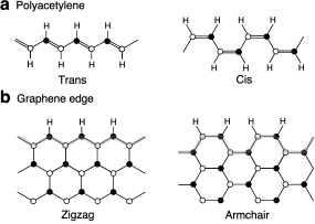
Figure 1: Structures of a polyacetylene and a graphene edge. a, Two possible isomers trans- and cis-polyacetylene. b, Two principal edge structures: zigzag and armchair edges. H denotes a hydrogen atom, and carbon atoms are divided into A ($\bullet$) and B ($\circ$) atoms.

(Definition of gauge fields)

First we review the chiral gauge theory of graphene. Sasaki and Saito (2008) A lattice deformation in graphene gives rise to a change of the nearest-neighbor hopping integral from the average value, $-\gamma$, as $-\gamma+\delta\gamma_{a}({\bf r})$, where $a$ $(=1,2,3)$ denotes the direction of a bond as shown in Fig. 2a. We define the axial gauge ${\bf A}({\bf r})=(A_{x}({\bf r}),A_{y}({\bf r}))$ by $\delta\gamma_{a}(\bf{r})$ as Kane and Mele (1997); Sasaki and Saito (2008); Katsnelson and Geim (2008)

$$\begin{split}&v_{\rm F}A_{x}({\bf r})=\delta\gamma_{1}({\bf r})-\frac{1}{2}\left\{\delta\gamma_{2}({\bf r})+\delta\gamma_{3}({\bf r})\right\},\\ &v_{\rm F}A_{y}({\bf r})=\frac{\sqrt{3}}{2}\left\{\delta\gamma_{2}({\bf r})-\delta\gamma_{3}({\bf r})\right\},\end{split}$$ (1)

where $v_{\rm F}$ is the Fermi velocity. The direction of the vector ${\bf A}({\bf r})$ is perpendicular to that of the C-C bond with a modified hopping integral, as shown in Fig. 2b. The effective Hamiltonian for a deformed graphene is written by a 4$\times$4 matrix as Sasaki and Saito (2008)

$${\hat{H}}\Psi({\bf r})=v_{\rm F}\begin{pmatrix}\mbox{\boldmath$\sigma$}\cdot\left({\bf{\hat{p}}}+{\bf A}({\bf r})-e{\bf A}^{\rm em}({\bf r})\right)&\sigma_{x}\phi({\bf r})\cr\sigma_{x}\phi^{*}({\bf r})&\mbox{\boldmath$\sigma$}^{\prime}\cdot\left({\bf{\hat{p}}}-{\bf A}({\bf r})-e{\bf A}^{\rm em}({\bf r})\right)\end{pmatrix}\begin{pmatrix}\Psi_{\rm K}({\bf r})\cr\Psi_{\rm K^{\prime}}({\bf r})\end{pmatrix},$$ (2)

where the field $\phi({\bf r})$ relates to ${\bf A}({\bf r})$ as $v_{\rm F}\phi({\bf r})=(A_{x}({\bf r})+iA_{y}({\bf r}))e^{-2ik_{\rm F}x}$ in which $k_{\rm F}$ is the Fermi wave vector of the K point, and ${\bf A}^{\rm em}({\bf r})$ is an electromagnetic gauge field. Here, $\mbox{\boldmath$\sigma$}=(\sigma_{x},\sigma_{y})$ [$\mbox{\boldmath$\sigma$}^{\prime}=(-\sigma_{x},\sigma_{y})$] are the Pauli matrices which operate on the two-component spinors $\Psi_{\rm K}({\bf r})$ and $\Psi_{\rm K^{\prime}}({\bf r})$ for the pseudospin. We use the units $v_{\rm F}=1$ and $\hbar=1$, and thus the momentum operator becomes ${\bf{\hat{p}}}=-i\nabla$. A lattice deformation does not break time-reversal symmetry, which appears as the different signs in front of the field ${\bf A}({\bf r})$ for the two chiralities, while the electromagnetic gauge field ${\bf A}^{\rm em}({\bf r})$ breaks time-reversal symmetry and has the same sign for the K and K^′ points. ${\bf A}$ (${\bf A}^{\rm em}$) is an axial (a vector) gauge field. Bertlmann (2000) Like the case of ${\bf A}^{\rm em}({\bf r})$, the field strength of ${\bf A}({\bf r})$ defined as $B_{z}({\bf r})=\partial_{x}A_{y}({\bf r})-\partial_{y}A_{x}({\bf r})$, plays a fundamental role in discussing topological solitons and edge states, as we will show below.

It is straightforward to show using equation (1) that the field $\phi$ behaves as a position-independent interaction for the Kekulé distortion, Sasaki and Saito (2008) and then equation (2) is equivalent to the Dirac equation with a mass $\phi$ in four-dimensional space-time without the $z$-component [$p_{z}=0$] (see Appendix A). Though the main concern of this paper is a chirality mixing due to a local mass $\phi({\bf r})$, let us begin by considering the massless limit $\phi({\bf r})=0$ and examining the chirality eigenstate $\Psi_{\rm K}$ (right-handed chirality) using the $2\times 2$ Hamiltonian, $H({\bf r})=\mbox{\boldmath$\sigma$}\cdot({\bf{\hat{p}}}+{\bf A}({\bf r}))$.

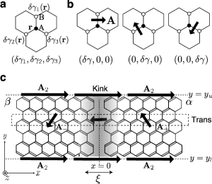
Figure 2: Representing a lattice deformation in terms of the axial (deformation-induced) gauge field. a, A lattice deformation is defined by $(\delta\gamma_{1},\delta\gamma_{2},\delta\gamma_{3})$. b, The direction of vector ${\bf A}$ is perpendicular to the lattice deformation. The directions of the arrows are for the case of a positive $\delta\gamma$. c, The configuration of the axial gauge field ${\bf A}$ for a trans zigzag nanoribbon. The two distinct bonding structures, $\alpha$ phase (${\bf A}_{+}$) and $\beta$ phase (${\bf A}_{-}$), are combined together to form a a domain wall (a kink). The $y$-component of the field ${\bf A}_{1}(x)$ changes its sign at $x=0$, which represents a kink structure. The zigzag edges are represented by the field ${\bf A}_{2}(y)$.

(Topology of the gauge field)

In Fig. 2c the double bond represents a shrinking of the C-C bond and the single bond denotes the absence of deformation. The $\alpha$ phase is defined as the bonding structure for the case of $(\delta\gamma_{1},\delta\gamma_{2},\delta\gamma_{3})=(0,\delta\gamma,0)$, while the $\beta$ phase is the case of $(\delta\gamma_{1},\delta\gamma_{2},\delta\gamma_{3})=(0,0,\delta\gamma)$. From equation (1), the corresponding ${\bf A}$ fields for the $\alpha$ and $\beta$ phases, ${\bf A}_{+}$ and ${\bf A}_{-}$, are given, respectively, by ${\bf A}_{\pm}=\left(-\delta\gamma/2,\pm\sqrt{3}\delta\gamma/2\right)$. For the skeleton of a trans-polyacetylene shown between the closed dashed lines of Fig. 2c, it is well-known that a topological soliton appears when the configuration has a domain wall (a kink), that is, when the $\beta$ phase changes into the $\alpha$ phase at some position along the $x$-axis. Su et al. (1979); Takayama et al. (1980); Heeger et al. (1988) The gauge field for such a domain wall configuration for a zigzag nanoribbon is written as

$${\bf A}_{1}(x)=(c_{x},A_{y}(x)),$$ (3)

where $c_{x}\equiv-\delta\gamma/2$, $A_{y}(x)=-a_{y}$ ($a_{y}\equiv\sqrt{3}\delta\gamma/2$) when $x\ll-\xi$, and $A_{y}(x)=a_{y}$ when $x\gg\xi$. Here, $\xi$ ($>0$) denotes the width of a kink (see Fig. 2c). In addition, the gauge field which describes the edge structure is given by ${\bf A}_{2}$. This ${\bf A}_{2}$ comes from the fact that the C-C bonds at the zigzag edge are cut. Sasaki et al. (2006) This cutting is represented by $(\delta\gamma_{1},\delta\gamma_{2},\delta\gamma_{3})=(\gamma,0,0)$ at the edge, and ${\bf A}_{2}=\left(\gamma,0\right)$. Since there are two zigzag edges at $y=y_{u}$ and $y=y_{l}$ in the zigzag nanoribbon (without a domain wall), ${\bf A}_{2}(y)=(A_{x}(y),0)$ has a value only for $y=y_{u}$ and $y=y_{l}$ (the edge location), and otherwise $A_{x}(y)=0$. The total gauge field for a trans zigzag nanoribbon is given by the sum of ${\bf A}_{1}(x)$ in equation (3) and ${\bf A}_{2}(y)$ as ${\bf A}_{1}(x)+{\bf A}_{2}(y)=(c_{x}+A_{x}(y),A_{y}(x))$. As a result, the (K point) Hamiltonian is given by

$$H({\bf r})=\sigma_{x}({\hat{p}}_{x}+c_{x}+A_{x}(y))+\sigma_{y}({\hat{p}}_{y}+A_{y}(x)).$$ (4)

(Zero-energy solution of $H({\bf r})$)

Here we assume that the energy eigenstates of $H({\bf r})$ in equation (4) has the form of $e^{ip_{x}x}\Psi_{p_{x}}(x,y)|\sigma\rangle$, where $p_{x}$ is the quantum number and $|\sigma\rangle$ denotes the spinor eigenstate. The energy eigenequation is rewritten as

$$\left\{\sigma_{x}({\hat{p}}_{x}+D_{x}+A_{x}(y))+\sigma_{y}({\hat{p}}_{y}+A_{y}(x))\right\}\Psi_{p_{x}}(x,y)|\sigma\rangle$$

$$=E\Psi_{p_{x}}(x,y)|\sigma\rangle,$$ (5)

where $D_{x}\equiv p_{x}+c_{x}$. We decompose this eigenequation into two parts by putting $\Psi_{p_{x}}(x,y)=\psi(x)\varphi(y)$ and $E=E_{1}+E_{2}$ as

$$\left\{\sigma_{x}{\hat{p}}_{x}+\sigma_{y}A_{y}(x)\right\}\psi(x)|\sigma\rangle=E_{1}\psi(x)|\sigma\rangle,$$ (6)

$$\left\{\sigma_{x}(D_{x}+A_{x}(y))+\sigma_{y}{\hat{p}}_{y}\right\}\varphi(y)|\sigma\rangle=E_{2}\varphi(y)|\sigma\rangle,$$ (7)

In general, the spinor eigenstate of the first equation can not be identical to that of the second one. However, in the special case that $E_{1}=E_{2}=0$, the spinor eigenstates of these equations can be the same. It is because that $H({\bf r})$ commutes with $\sigma_{z}$ for the zero-energy state, $\left[H({\bf r}),\sigma_{z}\right]_{-}e^{ip_{x}x}\Psi^{E=0}_{p_{x}}({\bf r})|\sigma\rangle=0$, and that the spinor eigenstate can be taken as the eigen spinor of $\sigma_{z}$ defined as $\sigma_{z}|\sigma_{\pm}\rangle=\pm|\sigma_{\pm}\rangle$, where

$$|\sigma_{+}\rangle=\begin{pmatrix}1\cr 0\end{pmatrix},\ \ |\sigma_{-}\rangle=\begin{pmatrix}0\cr 1\end{pmatrix}.$$

Thus, the corresponding zero-energy states are pseudospin polarized states, namely, the amplitude appears only one of the two sublattices. In the following, we show that equations (6) and (7) give, respectively, the topological soliton Su et al. (1979); Takayama et al. (1980); Heeger et al. (1988); Jackiw and Rebbi (1976) and the edge states. Sasaki et al. (2006); Sasaki and Saito (2008) From these zero-energy states for equations (6) and (7), a general zero-energy solution for equation (5) can be constructed.

(Topological soliton)

Let us obtain the zero-energy soliton for equation (6). When $E_{1}=0$, the eigenequation is represented as $\left\{\sigma_{x}{\hat{p}}_{x}+\sigma_{y}A_{y}(x)\right\}\psi_{\pm}(x)|\sigma_{\pm}\rangle=0$. We have two solutions,

$$\psi_{\pm}(x)=N\exp\left(\pm\int^{x}A_{y}(x)dx\right),$$ (8)

where $N$ is a normalization constant. When we use a trial function $A_{y}(x)=a_{y}\tanh(x/\xi)$, we get $\psi_{\pm}(x)=N\cosh^{\pm a_{y}\xi}(x/\xi)$. Rajaraman (1982) Hence, when $a_{y}>0$ (kink), only $\psi_{-}$ is selected, while when $a_{y}<0$ (anti-kink), only $\psi_{+}$ is selected. The significance of a single zero-energy state is that the particle-hole symmetric partner is given by itself, which leads to the result that a soliton has no charge but has spin $1/2$. Jackiw and Rebbi (1976); Heeger et al. (1988) The sign of $a_{y}$ corresponds to the sign of the field strength as $B_{z}(x)=a_{y}/(\xi\cosh^{2}(x/\xi))$. The sign of the $B_{z}$ field is essential to a rule for obtaining the normalizable solution. This is easy to understand by noting that the square of $H({\bf r})$ is given by $H({\bf r})^{2}=({\bf{\hat{p}}}+{\bf A}({\bf r}))^{2}+B_{z}({\bf r})\sigma_{z}$, which gives a positive coupling for $+B_{z}({\bf r})\sigma_{z}$. Because $H({\bf r})^{2}=0$ for a zero-energy state and $({\bf{\hat{p}}}+{\bf A}({\bf r}))^{2}$ is always a positive value, the zero-energy state needs to satisfy $+B_{z}({\bf r})\sigma_{z}<0$, so that a positive $B_{z}$ ($>0$) selects $|\sigma_{-}\rangle$ (or $\psi_{-}$) and a negative $B_{z}$ ($<0$) selects $|\sigma_{+}\rangle$ (or $\psi_{+}$).

(Edge states)

The derivation of the zero-energy edge states from equation (7) is given in Ref. Sasaki et al., 2006. For the case of $D_{x}<0$, there are degenerate zero-energy states given by

$$\begin{split}&\varphi_{+}(y)|\sigma_{+}\rangle=e^{D_{x}|y-y_{u}|}|\sigma_{+}\rangle,\\ &\varphi_{-}(y)|\sigma_{-}\rangle=e^{D_{x}|y-y_{l}|}|\sigma_{-}\rangle,\end{split}$$ (9)

where $|D_{x}|^{-1}$ is the localization length. As shown in Fig. 2c, at the upper edge located at $y=y_{u}$, the $A_{x}(y)$ field increases abruptly when $y$ approaches $y_{u}$ ($y\leq y_{u}$). Therefore, the corresponding $B_{z}$ field [$B_{z}(y)=-\partial_{y}A_{x}(y)$] is pointing toward the negative $z$-axis there. Hence, only the $|\sigma_{+}\rangle$ state can appear near the upper edge. In contrast, at the lower edge ($y=y_{l}$), the $A_{x}(y)$ field decreases abruptly as $y$ moves away from $y_{l}$ ($y\geq y_{l}$). Therefore, the corresponding field strength is positive there, and only the $|\sigma_{-}\rangle$ state is selected near the lower edge.

(Soliton-edge state)

A zero-energy solution of equation (5) is constructed by the product of the topological soliton $\psi_{-}(x)$ of equation (8) and the edge state $\varphi_{-}(y)|\sigma_{-}\rangle$ of equation (9) as

$$\Psi^{-}_{p_{x}}(x,y)|\sigma_{-}\rangle=e^{-\int^{x}A_{y}(x)dx}e^{D_{x}|y-y_{l}|}|\sigma_{-}\rangle.$$ (10)

This new state is localized not only near the lower zigzag edge but also near the kink. Since a kink satisfies $B_{z}(x)>0$, this state $\Psi^{-}_{p_{x}}(x,y)|\sigma_{-}\rangle$ is the solution to equation (5). If there is an anti-kink with $B_{z}(x)<0$ at $x=0$, another zero-energy state given by

$$\Psi^{+}_{p_{x}}(x,y)|\sigma_{+}\rangle=e^{+\int^{x}A_{y}(x)dx}e^{D_{x}|y-y_{u}|}|\sigma_{+}\rangle,$$ (11)

is the solution. This state is localized near another zigzag edge and is also localized near the anti-kink. In addition to these zero-energy solutions of the K point Hamiltonian, there are zero-energy solutions of the K^′ point Hamiltonian. Let the solutions for the K^′ point be of the form of $\Psi_{-p_{x}}(x,y)|\sigma\rangle=\psi^{\prime}(x)\varphi^{\prime}(y)|\sigma\rangle$. The energy eigenequation for the K^′ point Hamiltonian, $\mbox{\boldmath$\sigma$}^{\prime}\cdot({\bf{\hat{p}}}-{\bf A}({\bf r}))$, leads to a pair of energy eigenequations:

$$\begin{split}&\left\{\sigma_{x}{\hat{p}}_{x}+\sigma_{y}A_{y}(x)\right\}\psi^{\prime}(x)|\sigma\rangle=-E_{1}\psi^{\prime}(x)|\sigma\rangle,\\ &\left\{\sigma_{x}(D_{x}+A_{x}(y))+\sigma_{y}{\hat{p}}_{y}\right\}\varphi^{\prime}(y)|\sigma\rangle=E_{2}\varphi^{\prime}(y)|\sigma\rangle.\end{split}$$

These eigenequations are the same as those given in equations (6) and (7) (except for the unimportant sign change of $E_{1}$). As a result, the solutions to these equations are the same as equations (10) and (11). We thus have two zero-energy solutions originating from the K and K^′ points for a given $p_{x}$. This number of zero-energy states for a ribbon is different from a single zero-energy state for a polyacetylene chain. This difference is attributed to the fact that the soliton for a polyacetylene chain results from a chirality (or an intervalley) mixing.

(Chirality mixing)

The zero-energy solutions given by equations (10) and (11) have been obtained on the assumption that a chirality mixing between the K and K^′ points can be neglected. However, translational symmetry along the $x$-axis is broken due to the presence of a kink (or anti-kink) and a kink itself causes a mixing of chiralities. In this case, the eigenfunction may be written as a linear combination of $\Psi^{\pm}_{p_{x}}$ for the K point and $\Psi^{\pm}_{-p_{x}}$ for the K^′ point. Their mixing is determined by the mass term which is expressed by means of valleyspin $\tau_{a}$ ($a=0,1,2,3$) as $\sigma_{x}\left\{\tau_{1}{\rm Re}[\phi({\bf r})]-\tau_{2}{\rm Im}[\phi({\bf r})]\right\}$. By putting $\Psi_{\rm K}=e^{-ikx}\tilde{\Psi}_{\rm K}$ and $\Psi_{\rm K^{\prime}}=e^{+ikx}\tilde{\Psi}_{\rm K^{\prime}}$ into equation (2) for a zigzag ribbon, we obtain the equations for a general case:

$$\begin{split}&\left\{\tau_{3}\left(\sigma_{x}\hat{p}_{x}+\sigma_{y}A_{y}(x)\right)-\tau_{2}e^{i\tau_{3}2\delta kx}\sigma_{x}A_{y}(x)\right\}\tilde{\Psi}=E_{1}\tilde{\Psi},\\ &\tau_{0}\left\{\sigma_{x}(c_{x}-k+A_{x}(y))+\sigma_{y}\hat{p}_{y}\right\}\tilde{\Psi}=E_{2}\tilde{\Psi},\end{split}$$ (12)

where $\delta k\equiv k_{\rm F}-k$.  The last term on the left-hand side of the first equation of equation (12) shows that the effective domain wall profile for the mixing term is an oscillating function of $x$, in contrast to a smooth function of the intravalley mixing term for the second term. It is straightforward to find a zero-energy solution of equation (12) as $\tilde{\Psi}^{\pm}=U(x)\psi_{\pm}(x)\varphi_{\pm}(y)|\sigma_{\pm}\rangle$, where $U(x)$ is a matrix for valleyspin which satisfies the equation $\partial_{x}U(x)-\tau_{1}e^{i\tau_{3}2\delta kx}A_{y}(x)U(x)=0$. Due to the chirality mixing, the actual wave function of a zero-energy state in a zigzag nanoribbon can be complicated. One example of the wave function is shown in Fig. 3a.

(Soliton in polyacetylene)

Equation (12) can be solved analytically for the special case of $\delta k=0$ ($k=k_{\rm F}$). In this case, we obtain simultaneous differential equations:

$$\begin{split}&\sigma_{x}\left\{\frac{\tau_{3}}{2}\hat{p}_{x}-\tau_{2}A_{y}(x)\right\}\tilde{\Psi}=E_{1}\tilde{\Psi},\\ &\tau_{3}\left\{\frac{\sigma_{x}}{2}\hat{p}_{x}+\sigma_{y}A_{y}(x)\right\}\tilde{\Psi}=E_{2}\tilde{\Psi},\\ &\tau_{0}\left\{\sigma_{x}(c_{x}-k_{\rm F}+A_{x}(y))+\sigma_{y}\hat{p}_{y}\right\}\tilde{\Psi}=E_{3}\tilde{\Psi}.\end{split}$$ (13)

The first term gives rise to a chirality mixing. For a zero-energy solution of the first term, the spinor eigenstate should be the eigen spinor of $\tau_{1}$ defined as $\tau_{1}|\tau_{\pm}\rangle=\pm|\tau_{\pm}\rangle$, which shows a strong chirality mixing. The zero-energy solutions for the first two terms are given by $\tilde{\psi}_{\pm}(x)|\sigma_{\pm}\rangle\otimes|\tau_{\mp}\rangle$, where $\tilde{\psi}_{\pm}(x)=N\exp\left(\pm\int^{x}2A_{y}(x)dx\right)$. This state is a valleyspin unpolarized state and also a pseudospin polarized state, and these properties are consistent with those of the topological soliton in polyacetylene. Heeger and Schrieffer (1983) The third equation in equation (13) describes the edge state having the shortest localization length since the localization length is given by $|c_{x}-k_{\rm F}|^{-1}$ which vanishes in the continuum limit. The resulting zero-energy solution of equation (13) given by $\tilde{\Psi}({\bf r})=\tilde{\psi}_{\pm}(x)\varphi_{\pm}(y)|\sigma_{\pm}\rangle\otimes|\tau_{\mp}\rangle$ corresponds to Fig. 3b which reproduces a topological soliton in polyacetylene at the zigzag edge sites (see Fig. 3c for comparison). Note that the soliton can move along the zigzag edge and the soliton has a mass. In the case of polyacetylene, the soliton mass is estimated to be around $6m_{e}$, where $m_{e}$ is the mass of the free electron. Heeger and Schrieffer (1983) In the case of the ribbon, we obtain $65(W/\xi)m_{e}$, where $W$ denotes the ribbon width. This result reproduces the soliton mass in polyacetylene when $W=a$ and $\xi=10a$, where $a$ is the lattice constant.

Figure 3: Wave function patterns for zero-energy soliton. a, An example of the wave function pattern. The solid and empty circles represent the phases ($+$ or $-$) of the wave function, and the diameter of each circle is proportional to the amplitude. We use $\delta\gamma=0.2\gamma$ and the kink profile of $\tanh(x/\xi)$ with $\xi=2$Å. b, An example of the zero-energy soliton in a zigzag ribbon. Because the wave function of this example appears only at the edge sites, this state is identical to the topological soliton in a trans-polyacetylene shown in c.

To further elucidate the effect of the edge on the soliton, we consider the solitons of an armchair tube, a metallic zigzag tube, and a metallic armchair ribbon in Appendices B and C. We show that the chirality mixing is negligible for the zero-energy states in these tubes. A metallic armchair ribbon produces chirality mixed solitons when there is a domain wall. The solitons are not localized near the edge since there is no edge states near the armchair edge. This feature is in contrast to that of the soliton in a zigzag nanoribbon. See Appendices B and C for more details.

(Discussion)

We can use equation (1) for a lattice deformation induced by a strain. Let ${\bf u}({\bf r})=(u_{x}({\bf r}),y_{y}({\bf r}))$ be the displacement vector of a carbon atom at ${\bf r}$, the axial gauge field is written as Suzuura and Ando (2002); Guinea et al. (2010); Sasaki et al. (2010a)

$$\begin{split}&A_{x}({\bf r})=g\left[-\frac{\partial u_{x}({\bf r})}{\partial x}+\frac{\partial u_{y}({\bf r})}{\partial y}\right],\\ &A_{y}({\bf r})=g\left[\frac{\partial u_{x}({\bf r})}{\partial y}+\frac{\partial u_{y}({\bf r})}{\partial x}\right],\end{split}$$

where $g$ is the electron-phonon coupling. An interesting consequence of this is that the field configurations which are equivalent to ${\bf A}_{\pm}$ may be realized when an appropriate strain is applied to a sample. For example, a “${\rm V}$” shape graphene nanoribbon caused by an acoustic shear deformation given by $u_{x}=0$ and $u_{y}(x)=u\ln[\cosh(x/\xi)]$ with $u=\xi(a_{y}/g)$, can reproduce the gauge field representing a bond alternation (a domain wall) in zigzag ribbons. Because $g\simeq\gamma$, Sasaki et al. (2010a) $u$ is smaller than $\xi$ by a factor of $\delta\gamma/\gamma$. This shows that a domain wall can be realized by a strain of $\sim$ 10%. Guinea et al. (2010) Similarly, a strain produces a localized soliton in a metallic armchair nanoribbon (see Appendix C). On the other hand, the ribbon does not support the edge states without the strain. A pseudospin polarized wavefunction pattern that is spatially localized near the bottom of a “${\rm V}$” shape graphene nanoribbon is the indication of a chirality mixed soliton. Note that a strain makes it possible to observe the soliton by means of a scanning tunneling microscopy (STM) experiment, in contrast to that the STM is unable to detect a soliton in polyacetylene since the soliton is moving. Moreover, it was suggested recently by Guinea et al. Guinea et al. (2010) that a uniform $B_{z}$ field may be realized in graphene by a strain-induced lattice deformation, which is an interesting consequence. If this is the case, it is expected that the Landau level appears only for one chirality and the other chirality decouples from the gauge fields in the presence of a magnetic field which eliminates $B_{z}$ for one chirality. Then the chiral symmetry in graphene is maximally broken, and this situation is similar to the case of weak interactions in elementally particle physics.

Appendix A Original Dirac Hamiltonian

The original Dirac Hamiltonian is written as

$${\hat{H}}\Psi({\bf r})=\begin{pmatrix}\mbox{\boldmath$\sigma$}\cdot\left({\bf{\hat{p}}}+{\bf{\cal A}}({\bf r})+{\bf{\cal V}}({\bf r})\right)&m\cr m&-\mbox{\boldmath$\sigma$}\cdot\left({\bf{\hat{p}}}-{\bf{\cal A}}({\bf r})+{\bf{\cal V}}({\bf r})\right)\end{pmatrix}\begin{pmatrix}\Psi_{\rm R}({\bf r})\cr\Psi_{\rm L}({\bf r})\end{pmatrix},$$

where $m$ is the mass of fermion. The electronic Hamiltonian for graphene corresponds to the case in which $\Psi_{\rm R}\to\Psi_{\rm K}$, $\Psi_{\rm L}\to\sigma_{x}\Psi_{\rm K^{\prime}}$, and $m\to\phi({\bf r})$. The vector gauge field ${\bf{\cal V}}({\bf r})$ and axial gauge field ${\bf{\cal A}}({\bf r})$ correspond to $e{\bf A}^{\rm em}({\bf r})$ and ${\bf A}({\bf r})$, respectively. The third component such as ${\hat{p}}_{z}$ is assumed to be zero when we identify the original Dirac equation (in $3+1$ dimensional space-time) with the effective Hamiltonian for graphene (in $2+1$ dimensional space-time).

Appendix B Solitons in armchair nanotubes

Here we consider the solitons in armchair nanotubes. The K point Hamiltonian is given by removing $A_{x}(y)$ from equation (5). By putting $\Psi_{p_{x}}(x,y)=e^{-iD_{x}x}\psi(x)e^{ip_{y}y}$ into the energy eigenequation (5), we obtain $\left\{\partial_{x}\mp(p_{y}+A_{y}(x))\right\}\psi_{\pm}(x)=0$ for the zero-energy state. It follows that the function $\psi_{\pm}(x)$ contains the exponential function $\exp(\pm p_{y}x)$, so that either $\psi_{+}(x)$ with $p_{y}=0$ or $\psi_{-}(x)$ with $p_{y}=0$ can be a normalizable solution. The momentum $p_{y}$ is quantized by a periodic boundary condition around the tube’s axis, and a zero-momentum state $p_{y}=0$ satisfies the boundary condition for any armchair nanotube. Saito et al. (1992) The solution with $p_{y}=0$ is a topological soliton. From equation (2), we obtain the chirality mixing term as $\sigma_{x}\left\{\tau_{1}{\rm Re}[\phi(x)]-\tau_{2}{\rm Im}[\phi(x)]\right\}$, where $\phi(x)=iA_{y}(x)e^{-2ik_{\rm F}x}$. This mixing term is small because a smooth function $A_{y}(x)$ of $x$ is multiplied by a rapid oscillating function $e^{-2ik_{\rm F}x}$. Moreover, the chirality mixing term does not cause a first order energy shift since the unperturbed states $\psi_{\pm}(x)|\sigma_{\pm}\rangle$ are pseudospin polarized states satisfying $\langle\sigma_{\pm}|\sigma_{x}|\sigma_{\pm}\rangle=0$. For these reasons the chirality mixing is negligible in the case of an armchair nanotube.

Note that the zero-energy solitons in an armchair nanotube obtained above are distinct from the topological soliton in polyacetylene. The chirality mixing term is irrelevant to the solitons in armchair nanotubes, while it is relevant to the topological soliton in polyacetylene.

Appendix C Solitons in zigzag nanotubes and armchair ribbons

Let us examine solitons in a zigzag nanotube and an armchair ribbon. The existence of a zero-energy topological soliton in a zigzag tube requires two factors: the ${\bf A}$ field topology and the presence of the Dirac singularity. The ${\bf A}$ field topology can be understood by noting that the basic unit of structure is a cis-polyacetylene for which the two phases shown in Fig. 4a can be considered. Heeger et al. (1988) The $\alpha$ phase is defined by $(\delta\gamma_{1},\delta\gamma_{2},\delta\gamma_{3})=(0,\delta\gamma,\delta\gamma)$, and the $\beta$ phase is $(\delta\gamma_{1},\delta\gamma_{2},\delta\gamma_{3})=(\delta\gamma,0,0)$. From equation (1), the corresponding gauge fields for the $\alpha$ and $\beta$ phases, ${\bf A}_{+}$ and ${\bf A}_{-}$, are given, respectively, by ${\bf A}_{\pm}=\left(\mp\delta\gamma,0\right)$ [see Fig. 4b]. A domain wall kink is represented by ${\bf A}_{1}(y)=(A_{x}(y),0)$ with $A_{x}(y)=-\delta\gamma\tanh(y/\xi)$. By assuming that the wave function is of the form of $e^{ip_{y}y}\psi(x)\varphi(y)|\sigma\rangle$, we have a pair of the eigenequations from the K point Hamiltonian as

$$\begin{split}&\left\{\sigma_{x}A_{x}(y)+\sigma_{y}{\hat{p}}_{y}\right\}\varphi(y)|\sigma\rangle=E_{1}\varphi(y)|\sigma\rangle,\\ &\left\{\sigma_{x}{\hat{p}}_{x}+\sigma_{y}p_{y}\right\}\psi(x)|\sigma\rangle=E_{2}\psi(x)|\sigma\rangle.\end{split}$$

The first equation possesses a zero-energy topological soliton. Therefore, when there is a zero-energy state for the second equation, the K point Hamiltonian may possess a mixed zero-energy solution. The state with $p_{x}=0$ and $p_{y}=0$, i.e., the state at the Dirac singularity, can satisfy the second equation with $E_{2}=0$. Since $p_{x}$ is quantized by a periodic boundary condition around the tube’s axis, this state with vanishing wave vector exists only for “metallic” zigzag tubes. Saito et al. (1992) For “semiconducting” zigzag tubes, the quantized $p_{x}$ misses the Dirac singularity, and therefore such a zero-energy topological soliton does not exist. Thus, only the presence of a non-vanishing $B_{z}$ field strength does not necessarily result in the presence of a zero-energy state. In addition to a domain wall, the Dirac singularity is rather essential for the presence of a zero-energy state. Note that a non-topological excitation, a polaron, may exist even in “semiconducting” zigzag tubes near a bound kink-antikink pair. Heeger et al. (1988)

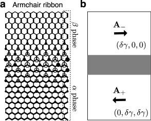
Figure 4: Soliton in an armchair nanoribbon. a, The wave function of a topological soliton in a metallic armchair nanoribbon obtained from a tight-binding model. b, The two phases ${\bf A}_{+}$ and ${\bf A}_{-}$ are separated by a domain wall kink distortion represented by the shaded region.

The localization pattern of a topological soliton is sensitive to the lattice structure of the edge of a nanoribbon. To illustrate this, we show the wave function of a topological soliton in a “metallic” armchair nanoribbon in Fig. 4a. The soliton is extended along the kink, which is contrasted with the localized feature of the wave function of a zero-energy state in a zigzag nanoribbon shown in Fig. 3a (in the text). This difference is a consequence of the fact that unrolling a zigzag tube can be represented by a strong intervalley mixing term $\phi({\bf r})$ at the armchair edge, and that this field $\phi({\bf r})$ does not destroy the Dirac singularity. Sasaki and Wakabayashi (2010) As a result, a topological soliton appears in a “metallic” armchair ribbon, as illustrated in Fig. 4a. It is interesting to note that unrolling a “metallic” zigzag tube does result in a “semiconducting” armchair ribbon. This implies that a topological soliton in a “metallic” zigzag tube disappears when the tube is unrolled since the Dirac singularity also disappears then.

References

- Sakurai (1967) J. Sakurai, Advanced Quantum Mechanics (Addison-Wesley, Canada, 1967).
- Bertlmann (2000) R. A. Bertlmann, Anomalies in Quantum Field Theory (Oxford Univ. Press, Oxford, 2000).
- Novoselov et al. (2005) K. S. Novoselov, A. K. Geim, S. V. Morozov, D. Jiang, M. I. Katsnelson, I. V. Grigorieva, S. V. Dubonos, and A. A. Firsov, Nature 438, 197 (2005).
- Zhang et al. (2005) Y. Zhang, Y.-W. Tan, H. Stormer, and P. Kim, Nature 438, 201 (2005).
- Wallace (1947) P. R. Wallace, Phys. Rev. 71, 622 (1947).
- Sasaki and Saito (2008) K. Sasaki and R. Saito, Prog. Theor. Phys. Suppl. 176, 253 (2008).
- Kane and Mele (1997) C. L. Kane and E. J. Mele, Phys. Rev. Lett. 78, 1932 (1997).
- Katsnelson and Geim (2008) M. Katsnelson and A. Geim, Phil. Trans. R. Soc. A 366, 195 (2008).
- Jackiw and Pi (2007) R. Jackiw and S.-Y. Pi, Phys. Rev. Lett. 98, 266402 (2007).
- Jia et al. (2009) X. Jia, M. Hofmann, V. Meunier, B. G. Sumpter, J. Campos-Delgado, J. M. Romo-Herrera, H. Son, Y.-P. Hsieh, A. Reina, J. Kong, et al., Science 323, 1701 (2009).
- Jiao et al. (2009) L. Jiao, L. Zhang, X. Wang, G. Diankov, and H. Dai, Nature 458, 877 (2009).
- Kosynkin et al. (2009) D. V. Kosynkin, A. L. Higginbotham, A. Sinitskii, J. R. Lomeda, A. Dimiev, B. K. Price, and J. M. Tour, Nature 458, 872 (2009).
- Chen et al. (2007) Z. Chen, Y.-M. Lin, M. J. Rooks, and P. Avouris, Physica E 40, 228 (2007).
- Stampfer et al. (2009) C. Stampfer, J. Güttinger, S. Hellmüller, F. Molitor, K. Ensslin, and T. Ihn, Phys. Rev. Lett. 102, 056403 (2009).
- Gallagher et al. (2010) P. Gallagher, K. Todd, and D. Goldhaber-Gordon, Phys. Rev. B 81, 115409 (2010).
- Han et al. (2010) M. Y. Han, J. C. Brant, and P. Kim, Phys. Rev. Lett. 104, 056801 (2010).
- Tanaka et al. (1987) K. Tanaka, S. Yamashita, H. Yamabe, and T. Yamabe, Synthetic Metals 17, 143 (1987).
- Fujita et al. (1996) M. Fujita, K. Wakabayashi, K. Nakada, and K. Kusakabe, J. Phys. Soc. Jpn. 65, 1920 (1996).
- Nakada et al. (1996) K. Nakada, M. Fujita, G. Dresselhaus, and M. S. Dresselhaus, Phys. Rev. B 54, 17954 (1996).
- Son et al. (2006) Y.-W. Son, M. L. Cohen, and S. G. Louie, Nature 444, 347 (2006).
- Pereira et al. (2006) V. M. Pereira, F. Guinea, J. M. B. L. dos Santos, N. M. R. Peres, and A. H. C. Neto, Phys. Rev. Lett. 96, 36801 (2006).
- Rice (1979) M. J. Rice, Phys. Lett. A 71, 152 (1979).
- Su et al. (1979) W. P. Su, J. R. Schrieffer, and A. J. Heeger, Phys. Rev. Lett. 42, 1698 (1979).
- Takayama et al. (1980) H. Takayama, Y. R. Lin-Liu, and K. Maki, Phys. Rev. B 21, 2388 (1980).
- Heeger et al. (1988) A. J. Heeger, S. Kivelson, J. R. Schrieffer, and W. P. Su, Rev. Mod. Phys. 60, 781 (1988).
- Sasaki et al. (2006) K. Sasaki, S. Murakami, and R. Saito, J. Phys. Soc. Jpn. 75, 074713 (2006).
- Jackiw and Rebbi (1976) R. Jackiw and C. Rebbi, Phys. Rev. D 13, 3398 (1976).
- Rajaraman (1982) R. Rajaraman, Solitons and instantons (Elsevier, North-Holland, 1982).
- Heeger and Schrieffer (1983) A. J. Heeger and J. R. Schrieffer, Solid State Communications 48, 207 (1983).
- Suzuura and Ando (2002) H. Suzuura and T. Ando, Phys. Rev. B 65, 235412 (2002).
- Guinea et al. (2010) F. Guinea, M. I. Katsnelson, and A. K. Geim, Nature Physics 6, 30 (2010).
- Sasaki et al. (2010a) K. Sasaki, H. Farhat, R. Saito, and M. S. Dresselhaus, Physica E 42, 2005 (2010a).
- Saito et al. (1992) R. Saito, M. Fujita, G. Dresselhaus, and M. S. Dresselhaus, Appl. Phys. Lett. 60, 2204 (1992).
- Sasaki and Wakabayashi (2010) K. Sasaki and K. Wakabayashi, arXiv:1003.5036 (2010).
- Sasaki et al. (2010b) K. Sasaki, K. Wakabayashi, and T. Enoki, arXiv:1002.4443 (2010b).