Bound-state effects on kinematical distributions
of top quarks at hadron colliders

Abstract:

First we present a theoretical framework to compute the fully differential cross sections for the top-quark productions and their subsequent decays at hadron colliders, incorporating the bound-state effects which are important in the $t\bar{t}$ threshold region. We include the bound-state effects such that the cross sections are correct in the LO approximation both in the threshold and high-energy regions. Then, based on this framework we compute various kinematical distributions of top quarks as well as of their decay products at the LHC, by means of Monte-Carlo event-generation. These are compared with the corresponding predictions based on conventional perturbative QCD. In particular, we find a characteristic bound-state effect on the $(bW^{+})$-$(\bar{b}W^{-})$ double-invariant-mass distribution, which is deformed to the lower invariant-mass side in a correlated manner.

1 Introduction

At the CERN Large Hadron Collider (LHC), the top quark will be produced copiously. The cross section for the top-quark pair-production amounts to several hundred pb [1, 2, 3], and order $10^{6}$ top-quark events will be observed each year if the LHC runs with 14 TeV collision energy and achieves the designed luminosity. Collecting these top-quark events, detailed analysis on the properties of the top quark will be possible, such as precise determinations of its mass and width, structure of electroweak and strong interactions, and its spin properties [4]. The current world average of the top-quark mass measurements from the combined analysis of CDF and D0 collaborations at the Fermilab Tevatron reads $m_{t}=173.1\pm 1.3$ GeV [5] (see also [6]). Furthermore, the top-quark production process is considered as a standard candle process. Namely, it serves understanding detector performances, e.g. jet energy calibrations, from comparisons of experimental measurements with theoretically reliable or well-controllable predictions, for observables including jet topologies, backgrounds and underlying events.

There have been many studies on top-quark production processes at the LHC. Update analyses on the total pair-production cross-section are presented in [1, 2, 3], including the next-to-leading-order (NLO) correction [7, 8] and resummation of threshold logarithms [9, 10, 11] in QCD. Differential distributions including decays of the top-quark have also been known up to NLO [12, 13, 14], and various distributions are investigated in [15, 16, 17, 18, 19].

Recently, $t\bar{t}$ invariant-mass ($m_{t\bar{t}}$) distribution near threshold has been investigated incorporating the bound-state effects [20, 21]. The effects are found to be significant at the LHC, since (in contrast to the Tevatron) the gluon-fusion channel dominates the cross section and there are significant contributions from (the remnant of) the color-singlet $t\bar{t}$ resonances.

In this paper we compute the fully differential cross sections for the top-quark pair productions and their subsequent decays at the LHC. In particular, we incorporate the bound-state effects, which are important in the $t\bar{t}$ threshold region, into the cross sections. We extend the studies of [20, 21] and present a theoretical frame to incorporate the bound-state effects to the differential cross sections. Using this result, we compute various kinematical distributions of the top quarks and their decay products at hadron colliders, by developing a Monte-Carlo (MC) event-generator incorporating the bound-state effects. (There exist similar MC event-generators for computing the top-quark cross-sections in the $t\bar{t}$ threshold region at future $e^{+}e^{-}$ colliders [22, 23, 24].) Through the analysis, we elucidate the nature of the bound-state effects at various stages: at the partonic matrix-element level, both with and without including the decay of the top quark, and in the kinematical distributions after incorporating the initial-state radiation (ISR) effects. Theoretically the fully differential cross sections contain more information on the bound-state effects than just the $t\bar{t}$ invariant-mass distribution; for instance, it is known that the top momentum distribution is sensitive to the resonance wave functions in momentum space [25, 26]. From a practical point of view, the differential cross sections are useful for studying effects of various kinematical cuts, detector acceptance corrections, detector calibrations, etc.

The method for incorporating $t\bar{t}$ bound-state effects has been developed mainly in the studies of $t\bar{t}$ productions in $e^{+}e^{-}$ collisions [27, 28, 29]. Formally, in the limit where we neglect the top-quark width, $\Gamma_{t}\to 0$, bound-state effects can be incorporated by resummation of the Coulomb singularities $(\alpha_{s}/\beta)^{n}$, where $\beta$ is the velocity of the top quark in the $t\bar{t}$ c.m. frame. In contrast to the $e^{+}e^{-}$ collision, at hadron colliders, $t\bar{t}$ pairs are produced in both color-singlet and octet states, and the (partonic) collision energy is not fixed. Due to the latter reason, we have to set up a theoretical framework which is valid both in the threshold region ($m_{t\bar{t}}\simeq 2m_{t}$) and in the high-energy region ($m_{t\bar{t}}\gg 2m_{t}$). The former region is where the bound-state effects (Coulomb corrections) become significant and where the non-relativistic approximation is valid. On the other hand, in the latter region, the bound-state effects are not significant and the top quarks are relativistic. We present a framework which takes into account all the leading-order (LO) corrections in both regions. Namely, we incorporate all the $(\alpha_{s}/\beta)^{n}$ terms in the threshold region, while we include all the $\beta^{n}$ terms in the relativistic region. (Some of the important subleading corrections are also incorporated.) Furthermore, we interpolate the two regions smoothly in a natural way.

Another important aspect in computing the differential cross sections for the top-quark productions and decays is to construct full amplitudes corresponding to the $bW^{+}\bar{b}W^{-}$ final state and to incorporate off-shellness of the top quarks appropriately [30]. The former is important to incorporate the polarizations of $t$ and $\bar{t}$ and angular correlations in their decay products. (In Appendix D, we will further discuss the polarizations of the $W$’s from the top quarks.) The latter is intimately related to the former and is known to be particularly important in the threshold region. In the $bW^{+}\bar{b}W^{-}$ production, there are non-resonant diagrams where $bW^{+}$ and $\bar{b}W^{-}$ are not produced from the decay of $t$ and $\bar{t}$. Often the non-resonant diagrams are omitted in the studies of $t\bar{t}$ productions, since they are suppressed in the events where both $t$ and $\bar{t}$ are nearly on-shell. In the threshold region, however, either of $t$ and $\bar{t}$ tends to be off-shell due to restricted phase-space and the binding effects [25], and the non-resonant diagrams can give non-negligible contributions compared to the resonant ($t\bar{t}$) diagrams [31]. Since these contributions interfere with each other, all the diagrams have to be taken into account at the amplitude level. Moreover, because of the requirement by unitarity, we also have to ensure a consistent treatment of the finite decay width of the top quark in our framework. We will discuss these points within our framework, which includes the bound-state effects as well as the non-resonant diagrams, in connection with a known problem regarding a gauge cancellation.

In order to compute numerically various kinematical distributions at hadron colliders, we develop a MC event-generator, which is adapted to the MadEvent [32, 33] environment. We include the bound-state effects in the hard-scattering part of the LO event-generator, on the basis of our theoretical framework. The ISR and/or final-state radiation (FSR), which are of importance at hadron colliders, are incorporated via the parton-shower approach. Since the parton shower does not alter the normalizations of the cross sections at the partonic level, we will complement the overall normalizations, known up to NLO [20, 21], by multiplying the cross sections in the individual channels with the so-called “$K$-factors.” We note, however, that our aim here is to construct a generator valid only up to LO with respect to the differential distributions, in this first attempt to include the bound-state effects. Compare with the existing NLO event-generators, such as MC@NLO [34, 35] and POWHEG [36], which realize a consistent treatment of perturbative corrections for any process and any phase-space point.

Using the generated events, we study the bound-state effects on the top quark differential distributions at the LHC, focusing on the events in a relatively low $m_{t\bar{t}}$ region. A $t\bar{t}$ pair gains a binding energy due to exchange of Coulomb gluons between them. This effect tends either of $t$ and $\bar{t}$ to be off-shell below the threshold, and the effect remains even a few tens GeV above the threshold, due to the large width of the top quark. We will quantify this picture through detailed examinations of the top quark differential distributions.

The paper is organized as follows. In Sec. 2, we give a theoretical framework for computing the amplitudes for top-quark pair-production at hadron colliders, incorporating the bound-state effects (Sec. 2.1), the finite width effects (Sec. 2.2), and the ISR effects and $K$-factors (Sec. 2.3). In Sec. 3, we present numerical studies for various kinematical distributions in $t\bar{t}$ production, using the MC simulation which implements the ingredients explained in the previous section. In Sec. 4, we summarize our results. To avoid complexity in the main body of the paper, several detailed discussions are presented in the Appendices. In App. A, we identify the $t\bar{t}$ Green function in a Feynman amplitude. In App. B, we derive the off-shell suppression factor. In App. C, the color decomposition of the amplitude is explained. In App. D, we examine the leptonic decays of $W$’s from top quarks with and without spin correlations.

2 Inclusion of Bound-state Effects

In this section we present a theoretical investigation of how to include the $t\bar{t}$ bound-state effects in the matrix elements for $gg\to bW^{+}\bar{b}W^{-}$ and $q\bar{q}\to bW^{+}\bar{b}W^{-}$. In particular we include the effects such that the amplitude is correct in the leading-order approximation both in the $t\bar{t}$ threshold region and in the high energy region. Inclusion of several different effects is explained in steps: In Sec. 2.1 we explain how to incorporate the bound-state effects; in Sec. 2.2 important higher-order effects of the large top-quark decay-width are incorporated; in these subsections, we consider only the partonic $S$-matrix elements. In Sec. 2.3 we incorporate the ISR effects and the $K$-factors in the corresponding partonic differential cross sections.

For later convenience, we divide each amplitude into two parts, the $t\bar{t}$ (double-resonant) part and the non-resonant part, as

$${\cal M}^{(c)}(I\to bW^{+}\bar{b}W^{-})={\cal M}^{(c)}_{t\bar{t}}(I\to t\bar{t}\to bW^{+}\bar{b}W^{-})+{\cal M}^{(c)}_{\rm nr}(I\to bW^{+}\bar{b}W^{-})\,,$$ (1)

where $I=gg$ or $q\bar{q}$ represents initial-state partons, and $c$ represents the color ($c=1$ and 8 for the singlet and octet, respectively) of $I$, or equivalently, of $b\bar{b}$ in the final-state. The first term on the right-hand side represents the sum of the diagrams which contain both $t$ and $\bar{t}$ as an intermediate state. This part of the amplitude consists of $I\to t\bar{t}$ processes followed by subsequent decays of $t$ and $\bar{t}$. The second term represents the sum of the rest of the diagrams, which consists of single(-top)-resonant diagrams and non-resonant diagrams. Fig. 1 shows the tree-level Feynman diagrams for the processes $gg\to t\bar{t}$ and $q\bar{q}\to t\bar{t}$.

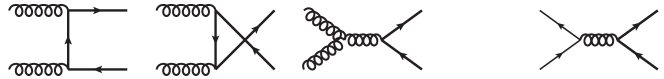
Figure 1: Feynman diagrams for $gg\to t\bar{t}$ and $q\bar{q}\to t\bar{t}$ at the tree-level.

Some examples of the tree-level diagrams included in each part for $I=gg$ are shown in Fig. 2.

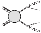
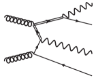
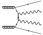
Figure 2: Typical Feynman diagrams for the double-resonant (left), single-resonant (middle) and non-resonant (right) contributions in the $gg\to bW^{+}\bar{b}W^{-}$ process. They belong to ${\cal M}^{(c)}_{t\bar{t}}$, ${\cal M}_{\rm nr}^{(c)}$ and ${\cal M}_{\rm nr}^{(c)}$, respectively. The term “resonant” is used to refer to the $t$ or $\bar{t}$ quark propagator (shown with double line) which can become close to on-shell. The blob in the left diagram represents the first three diagrams in Fig. 1.

In general each part is gauge-dependent. In this paper, we work in Feynman gauge for $SU(3)_{\rm c}$ and in unitary gauge for the broken electroweak symmetry.

In computing the tree-level Feynman diagrams which contain the top-quark propagators, we include the (on-shell) top-quark decay-width $\Gamma_{t}$ in the propagator denominator as

$${\cal S}_{F}(p_{t})=\frac{i(p/_{t}+m_{t})}{p_{t}^{2}-m_{t}^{2}+im_{t}\Gamma_{t}}\,.$$ (2)

2.1 LO cross section valid from threshold to high energies

In this subsection we include the bound-state effects in the $t\bar{t}$ amplitude ${\cal M}_{t\bar{t}}^{(c)}$. We consider the narrow-width limit of top-quark width in this subsection. Namely, we take into account only the leading contributions as $\Gamma_{t}\to 0$. Important subleading effects by the finite top-quark width will be investigated separately in the next subsection.

We start by reviewing the conventional method for including the bound-state effects in the matrix element (or in the fully differential cross section) of $e^{+}e^{-}\to t\bar{t}\to bW^{+}\bar{b}W^{-}$ close to the threshold of $t\bar{t}$ pair productions. At the leading-order, this is achieved by multiplying the tree-level amplitude corresponding to the diagrams $e^{+}e^{-}\to t\bar{t}\to bW^{+}\bar{b}W^{-}$ by an enhancement factor as [25, 26]

$${\cal M}(e^{+}e^{-}\to t\bar{t}\to bW^{+}\bar{b}W^{-})={\cal M}(e^{+}e^{-}\to t\bar{t}\to bW^{+}\bar{b}W^{-})_{\rm tree}$$

$$\times\frac{G^{(1)}(E+i\Gamma_{t},\vec{p})}{G_{0}(E+i\Gamma_{t},\vec{p})}.$$ (3)

Here, the non-relativistic Green functions are defined by

$$\left[(E+i\Gamma_{t})-\left\{-\frac{\nabla^{2}}{m_{t}}+V_{\rm QCD}^{(c)}(r)\right\}\right]\tilde{G}^{(c)}(E+i\Gamma_{t},\vec{r})=\delta^{3}(\vec{r}),$$ (4)

$$G^{(c)}(E+i\Gamma_{t},\vec{p})=\int d^{3}\vec{r}\,e^{-i\vec{p}\cdot\vec{r}}\,\tilde{G}^{(c)}(E+i\Gamma_{t},\vec{r})\,.$$ (5)

$E=\sqrt{s}-2m_{t}$ is the c.m. energy measured from the threshold; $m_{t}$ is the pole mass of the top quark; $\vec{r}$ denotes the relative coordinate of $t$ and $\bar{t}$, while $\vec{p}$ denotes the three-momentum of $t$ (or minus the three-momentum of $\bar{t}$), both defined in the c.m. frame; $V_{\rm QCD}^{(c)}(r)$ is the QCD potential between the $t\bar{t}$ pair in the color-singlet ($c=1$) or color-octet ($c=8$) channel. In $e^{+}e^{-}$ collisions, $t\bar{t}$ pairs are produced in the color-singlet channel, hence $c=1$ in Eq. (3). The free non-relativistic Green function $G_{0}(E+i\Gamma_{t},\vec{p})$ is obtained from $G^{(c)}(E+i\Gamma_{t},\vec{p})$ by setting $V_{\rm QCD}^{(c)}(r)\to 0$. Formally the above Green function can be expressed as

$$G^{(c)}(E+i\Gamma_{t},\vec{p})=\left<{\vec{p}\rule[-5.69054pt]{0.0pt}{17.07164pt}}\,\right|\frac{1}{E+i\Gamma_{t}-\vec{p}^{\,2}/m_{t}-V_{\rm QCD}^{(c)}(r)}\left|\,{\vec{r}=\vec{0}}\,\right>,$$ (6)

using an operator notation in quantum mechanics. By definition, the above Green function contains only the $S$-wave contributions.

There are two methods to compute the total cross section for $e^{+}e^{-}\to t\bar{t}\to bW^{+}\bar{b}W^{-}$ incorporating the bound-state effects. One way is to integrate the absolute square of the matrix element given in Eq. (3) over the phase-space of the final $bW^{+}\bar{b}W^{-}$ state. The other method is to use the optical theorem (unitarity relation) and take the imaginary part of a current-current correlator (two-point function). At the leading-order, the latter method leads to the formula [27, 28]:

$$\sigma_{\rm tot}(e^{+}e^{-}\to t\bar{t}\to bW^{+}\bar{b}W^{-})=\sigma_{\rm tot}(e^{+}e^{-}\to t\bar{t})_{\rm tree}~{}~{}~{}~{}~{}~{}~{}~{}~{}~{}~{}~{}~{}~{}~{}~{}$$

$$\times\frac{\mathop{\rm Im}\Bigl{[}\tilde{G}^{(1)}(E+i\Gamma_{t},\vec{r}=\vec{0})\Bigr{]}}{\mathop{\rm Im}\Bigl{[}\tilde{G}_{0}(E,\vec{r}=\vec{0})\Bigr{]}},$$ (7)

where the Green function in coordinate space is defined in Eq. (4). $\sigma_{\rm tot}(e^{+}e^{-}\to t\bar{t})_{\rm tree}$ denotes the Born cross-section for the production of on-shell top quarks. Note that in the denominator we set $\Gamma_{t}$ to zero in $\tilde{G}_{0}$, whereas $\Gamma_{t}$ is retained in the denominator in Eq. (3). The different treatment of $\Gamma_{t}$ is because in Eq. (3) we use the tree-level amplitude with unstable top quarks (in the intermediate state), whereas in Eq. (7) we use the tree-level cross section of the on-shell top quarks (in the final state).

Both formulas (3) and (7) incorporate all the leading-order corrections $\sim(\alpha_{s}/\beta)^{n}$ in the threshold region $E\ll m_{t}$. On the other hand, the formulas are not valid at higher c.m. energies $E\hbox{ \raise 3.0pt\hbox to0.0pt{$>$}\raise-3.0pt\hbox{$\sim$} }m_{t}$, since relativistic corrections $\sim\beta^{n}$, which grow with energy, are neglected in these formulas.

Now we turn to the partonic cross sections for the top-quark productions in hadron collisions, $I\to t\bar{t}\to bW^{+}\bar{b}W^{-}$ with $I=gg$ and $q\bar{q}$. Unlike $e^{+}e^{-}$ collisions, the collision energy of the initial state cannot be fixed. Thus, we need to consider both threshold and high-energy regions. The formulas which we propose, valid in both regions within the leading-order approximation, can be summarized as follows:

• The $t\bar{t}$ amplitude for $I\to t\bar{t}\to bW^{+}\bar{b}W^{-}$ is given by

  $${\cal M}^{(c)}_{t\bar{t}}(I\to t\bar{t}\to bW^{+}\bar{b}W^{-}) = {\cal M}^{(c)}_{t\bar{t}}(I\to t\bar{t}\to bW^{+}\bar{b}W^{-})_{\rm tree}$$ (8)

  $$~{}~{}~{}~{}~{}~{}~{}~{}~{}~{}~{}~{}~{}~{}~{}~{}~{}\times\frac{G^{(c)}(E^{\prime}+i\Gamma_{t},\vec{p})}{G_{0}(E^{\prime}+i\Gamma_{t},\vec{p})},$$

  with

  $$E^{\prime}=E+\frac{E^{2}}{4m_{t}}\,.$$ (9)

  The Feynman diagrams which contribute to the tree-level amplitude ${\cal M}^{(c)}_{t\bar{t}}(I\to t\bar{t}\to bW^{+}\bar{b}W^{-})_{\rm tree}$ are those shown in Fig. 1, after attaching the decay vertices $t\to bW^{+}$ and $\bar{t}\to\bar{b}W^{-}$ to each diagram. There are both color-singlet ($c=1$) and color-octet ($c=8$) channels in the case $I=gg$, while there is only the color-octet channel in the case $I=q\bar{q}$. Here, $E$ is defined from the $t\bar{t}$ invariant-mass $m_{t\bar{t}}$ as $E=m_{t\bar{t}}-2m_{t}$. The only essential difference from the corresponding formula for the $e^{+}e^{-}$ collision, Eq. (3), is the use of the modified energy $E^{\prime}$ [Eq. (9)] instead of $E$.
  

• We may compute the $t\bar{t}$ invariant-mass distribution by integrating the absolute square of the above amplitude $|{\cal M}^{(c)}_{t\bar{t}}(I\to t\bar{t}\to bW^{+}\bar{b}W^{-})|^{2}$ over the $bW^{+}\bar{b}W^{-}$ phase-space for each fixed $m_{t\bar{t}}$. Alternatively we may obtain the formula for the $t\bar{t}$ invariant-mass distribution using the optical theorem, similarly to the $e^{+}e^{-}\to t\bar{t}$ case. In the leading-order approximation, this reads

  $$\hat{\sigma}_{\rm tot}^{(c)}(I\to t\bar{t}\to bW^{+}\bar{b}W^{-})=\hat{\sigma}_{\rm tot}^{(c)}(I\to t\bar{t})_{\rm tree}\times\frac{\mathop{\rm Im}\Bigl{[}\tilde{G}^{(c)}(E^{\prime}+i\Gamma_{t},\vec{r}=\vec{0})\Bigr{]}}{\mathop{\rm Im}\Bigl{[}\tilde{G}_{0}(E^{\prime},\vec{r}=\vec{0})\Bigr{]}}\,.$$

  (10)

  As in the $e^{+}e^{-}\to t\bar{t}$ case, $\hat{\sigma}_{\rm tot}^{(c)}(I\to t\bar{t})_{\rm tree}$ is the Born cross-section for the on-shell top quarks; accordingly $\Gamma_{t}$ is set to zero in $\tilde{G}_{0}(E^{\prime},\vec{r}=\vec{0}\bigr{)}$. We note that the $t\bar{t}$ invariant-mass distribution obtained from Eq. (10) does not exactly coincide with that obtained by integrating $|{\cal M}^{(c)}_{t\bar{t}}(I\to t\bar{t}\to bW^{+}\bar{b}W^{-})|^{2}$ over the $bW^{+}\bar{b}W^{-}$ phase-space; the difference is ${\cal O}(\Gamma_{t}/m_{t})$ and will be discussed in the next subsection.

In the following we sketch our theoretical consideration which led to the above formulas (8) and (10), where some details are relegated to App. A. As explained in that appendix, part of the Feynman amplitude for $I\to t\bar{t}\to bW^{+}\bar{b}W^{-}$ can be identified with a Green function that dictates the time evolution of the $t\bar{t}$ system. (Such an identification is possible in all kinematical regions.) In the c.m. frame of $t\bar{t}$, for the initial-state $\left|\,{i}\,\right>$ and final-state $\left|\,{f}\,\right>$ of the $t\bar{t}$ system, this Green function can be written formally as

$$\left<{f}\,\right|\frac{1}{m_{t\bar{t}}-H+i\Gamma_{t}}\left|\,{i}\,\right>,$$ (11)

where $m_{t\bar{t}}$ is the c.m. energy of $t\bar{t}$ ($t\bar{t}$ invariant-mass). The full QCD Hamiltonian is denoted by $H$. Because of this property, the amplitude for $I\to t\bar{t}\to bW^{+}\bar{b}W^{-}$, which incorporates the $t\bar{t}$ bound-state effects, can be obtained from the tree-level amplitude by multiplying an enhancement factor:

$${\cal M}^{(c)}_{t\bar{t}}(I\to t\bar{t}\to bW^{+}\bar{b}W^{-})\approx{\cal M}^{(c)}_{t\bar{t}}(I\to t\bar{t}\to bW^{+}\bar{b}W^{-})_{\rm tree}~{}~{}~{}~{}~{}~{}~{}~{}$$

$$\times\frac{\displaystyle\left<{\vec{p}\rule[-5.69054pt]{0.0pt}{17.07164pt}}\,\right|\frac{1}{m_{t\bar{t}}-H+i\Gamma_{t}}\left|\,{\vec{r}=\vec{0}}\,\right>}{\displaystyle\left<{\vec{p}\rule[-5.69054pt]{0.0pt}{17.07164pt}}\,\right|\frac{1}{m_{t\bar{t}}-H_{0}+i\Gamma_{t}}\left|\,{\vec{r}=\vec{0}}\,\right>}.$$ (12)

$H_{0}$ denotes the Hamiltonian $H$ after setting $\alpha_{s}\to 0$, i.e. the free Hamiltonian. As before, $\vec{r}$ denotes the relative coordinate of $t$ and $\bar{t}$, while $\vec{p}$ denotes the three-momentum of $t$, both defined in the c.m. frame of the $t\bar{t}$ system. Corrections to Eq. (12), which come from the non-resonant part of the amplitude (i.e. that vanish as $\Gamma_{t}\to 0$), are neglected; see Appendix A.

In the above equation, we have taken advantage of the fact that we work in the leading-order approximation and set the initial-state of the Green functions as $|\vec{r}=\vec{0}\rangle$. This follows from the following consideration. Naively, the $t\bar{t}$ system cannot be regarded as being created by contact interaction (i.e. at the same point $\vec{r}=\vec{0}$) in the $t$- and $u$-channel diagrams of $gg\to t\bar{t}$, in which the top-quark is exchanged between the initial $gg$ (see Fig. 1). In the non-relativistic region, however, we may set $\vec{p}\to 0$ in the $t$- or $u$-channel top-quark propagator in the leading-order approximation. The denominator of the propagator effectively reduces to a constant close to the threshold, so that $t\bar{t}$ can be regarded as being created at the same point. On the other hand, in the relativistic region the enhancement factor in Eq. (12) reduces to $1+{\cal O}(\alpha_{s})$. Hence, it is justified to evaluate the Green functions with the initial-state $|\vec{r}=\vec{0}\rangle$ within our present approximation.

Since our aim is to include the leading-order contributions both in the relativistic and non-relativistic regions, the full form of the Hamiltonian is not necessary. In the region where $t$ and $\bar{t}$ are relativistic, $m_{t\bar{t}}-2m_{t}\hbox{ \raise 3.0pt\hbox to0.0pt{$>$}\raise-3.0pt\hbox{$\sim$} }m_{t}$, the leading-order contribution in the Hamiltonian reads

$$H=2\sqrt{\vec{p}^{\,2}+m_{t}^{2}}+{\cal O}(\alpha_{s})\,,$$ (13)

as shown in Appendix A. It is nothing but the sum of the energies of free on-shell $t$ and $\bar{t}$. The above equation also indicates how the next-to-leading order effects enter the Hamiltonian. On the other hand, in the non-relativistic region, $E=m_{t\bar{t}}-2m_{t}\ll m_{t}$, the leading-order contributions in the Hamiltonian can be written explicitly as

$$H=2m_{t}+\Biggl{[}\frac{\vec{p}^{\,2}}{m_{t}}+V_{\rm QCD}^{(c)}(r)\Biggr{]}\times\Bigl{[}1+{\cal O}(\alpha_{s},\beta)\Bigr{]}.$$ (14)

It is indicated that the next-to-leading order corrections enter as ${\cal O}(\beta)$ relativistic corrections or ${\cal O}(\alpha_{s})$ corrections.

A natural choice of the Hamiltonian, which incorporates the leading-order contributions in both regions and smoothly interpolates these regions, is given by

$$H_{\rm LO}=2\sqrt{\vec{p}^{\,2}+m_{t}^{2}}+V^{(c)}_{\rm QCD}(r).$$ (15)

In fact, it is well known that, when computing higher-order corrections in Coulombic bound-state problems, part of them (relativistic corrections) contribute exactly in the above form [37]. Thus, in principle, one may determine the enhancement factor in Eq. (12) using the above Hamiltonian.

Due to technical reasons, however, we use an alternative form of the enhancement factor, which is equivalent within the present approximation. By substituting $E=m_{t\bar{t}}-2m_{t}$ to the on-shell relation

$$m_{t\bar{t}}=2\sqrt{\vec{p}^{\,2}+m_{t}^{2}},$$ (16)

one finds that

$$E+\frac{E^{2}}{4m_{t}}=\frac{\vec{p}^{\,2}}{m_{t}}.$$ (17)

Therefore, if we define

$$G^{(c)}\bigl{(}E^{\prime}+i\Gamma_{t},\vec{p}\bigr{)}=\left<{\vec{p}\rule[-5.69054pt]{0.0pt}{17.07164pt}}\,\right|\frac{1}{E^{\prime}+i\Gamma_{t}-(\vec{p}^{\,2}/m_{t}+V^{(c)}_{\rm QCD}(r))}\left|\,{\vec{r}=\vec{0}}\,\right>$$ (18)

with $E^{\prime}$ defined by Eq. (9), the position of the pole of $G^{(c)}(E^{\prime}+i\Gamma_{t},\vec{p})$ is the same as that of $\langle\vec{p}|(m_{t\bar{t}}-H_{\rm LO}+i\Gamma_{t})^{-1}|\vec{r}=\vec{0}\rangle$ in the limit $\alpha_{s}\to 0$. Furthermore, in the non-relativistic region, evidently $G^{(c)}(E^{\prime},\vec{p})$ is the same as $\langle\vec{p}|(m_{t\bar{t}}-H_{\rm LO}+i\Gamma_{t})^{-1}|\vec{r}=\vec{0}\rangle$ in the leading-order approximation. Hence, we may compute the matrix element by the formula Eq. (8). One may be worried that, although the replacement $E\to E^{\prime}$ correctly accounts for the pole position, the residue of the pole may be altered significantly from that of Eq. (12) in the relativistic region. This is not the case, since the change of the residue will be canceled in the ratios of the Green functions in Eqs. (8) and (10).

The advantage of using $G^{(c)}(E^{\prime}+i\Gamma_{t},\vec{p})$ is that one can obtain it from the conventional non-relativistic Green function with a minimal modification $E\to E^{\prime}=E+{E^{2}}/({4m_{t}})$. In particular, properties of $G^{(c)}$ are fairly well known.

Let us comment on the dependence of the Green function on the top-quark width $\Gamma_{t}$ in Eq. (18). In Eq. (2) the shift of the pole position of the top-quark propagator due to the finite top-quark width can be incorporated simply by a replacement $m_{t}^{2}\to m_{t}^{2}-im_{t}\Gamma_{t}$. If we apply it to Eq. (16), one finds that $i\Gamma_{t}$ will be added to the left-hand side of Eq. (17). Hence, inclusion of $\Gamma_{t}$ as in Eq. (18) is correct in the leading-order approximation.

Throughout our analysis, we include an important subleading correction to the bound-state effects, in order to make our analysis more realistic. This is the NLO (1-loop) correction to the static potentials $V^{(c)}_{\rm QCD}(r)$ between the $t\bar{t}$ pair. The NLO potential reads [38]

$$V_{\rm QCD}^{(c)}(r;\mu_{\rm B})=C^{(c)}\frac{\alpha_{s}(\mu_{\rm B})}{r}\left[1+\frac{\alpha_{s}(\mu_{\rm B})}{4\pi}\left\{2\beta_{0}\left[\ln(\mu_{\rm B}r)+\gamma_{E}\right]+a_{1}^{(c)}\right\}\right]$$ (19)

with

$$C^{(1)}=-C_{F},~{}~{}~{}~{}C^{(8)}=\frac{C_{A}}{2}-C_{F},$$ (20)

$$\beta_{0}=\frac{11}{3}C_{A}-\frac{2}{3}n_{q},~{}~{}~{}~{}~{}a_{1}^{(1)}=a_{1}^{(8)}=\frac{31}{9}C_{A}-\frac{10}{9}n_{q},$$ (21)

for the $\overline{\rm MS}$ coupling. Here, $\gamma_{E}=0.5772...$ denotes the Euler constant; $C_{F}=4/3$ and $C_{A}=3$ are color factors. The QCD potential is renormalization-group invariant, and we evaluate the above expression at the Bohr scale of $\mu_{\rm B}=20$ GeV and with $n_{q}=5$ ($\alpha_{s}(\mu_{B})=0.153$).

Now we perform a few tests of our formulas, Eqs. (8) and (10). First we examine the impact of the replacement $E\to E^{\prime}$. The $t\bar{t}$ invariant-mass distributions $d\hat{\sigma}/dm_{t\bar{t}}$ computed with these formulas are compared with $d\hat{\sigma}/dm_{t\bar{t}}$ computed by the formulas valid only in the threshold region, namely Eqs. (8) and (10) after we replace $E^{\prime}$ by $E$.

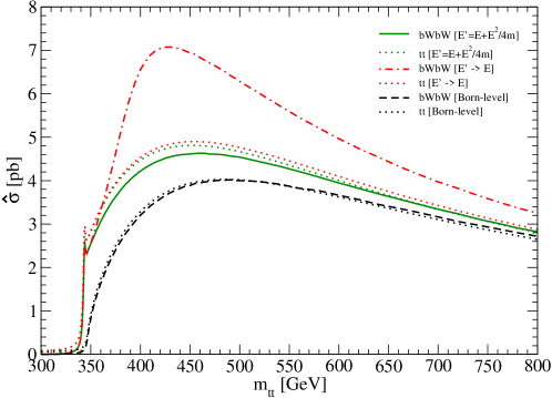
Figure 3: Partonic $t\bar{t}$ invariant-mass distributions for $gg\to t\bar{t}\to bW^{+}\bar{b}W^{-}$ in the color-singlet channel. The green solid line is calculated with $E^{\prime}=E+E^{2}/(4m_{t})$ [Eq. (9)], while the red dot-dashed line is calculated with $E$ instead of $E^{\prime}$. The black dashed line represents the Born cross-section. The dotted lines are those for the $gg\to t\bar{t}$ process (production of on-shell top quarks).

In Fig. 3 we plot $\hat{\sigma}$ for $gg\to t\bar{t}$ in the color-singlet channel. The green solid and dotted lines are those computed using Eqs. (8) and (10), respectively, while the red dot-dashed and dotted lines are those computed with the same formulas but after the replacement $E^{\prime}\to E$. For comparison, the Born cross-sections [using Eqs. (8) and (10) but without the enhancement factors] are also plotted with the dashed and dotted black lines. All the cross sections are computed with $m_{t}=173$ GeV and $\Gamma_{t}=1.49$ GeV (the tree-level top-quark decay-width).

The difference between the $t\bar{t}$ invariant-mass distributions using Eqs. (8) and (10) (solid and dotted green lines) is due to ${\cal O}(\Gamma_{t}/m_{t})$ corrections. The replacement $E^{\prime}\to E$ in Eq. (10) changes the $t\bar{t}$ invariant-mass distribution slightly above the $t\bar{t}$ threshold; compare the green dotted and red dotted lines. The difference between the two cross sections is about 2.5% in the large $m_{t\bar{t}}$ region.

On the other hand, the effect of the replacement $E^{\prime}\to E$ in Eq. (8) is much more pronounced above the $t\bar{t}$ threshold. There exist a large enhancement which amounts to nearly a factor of two around $m_{t\bar{t}}=400$ GeV; compare the green solid and red dot-dashed lines. The origin of this large enhancement can be identified with a mismatch of the on-shell conditions satisfied by the pole positions of the $t$ and $\bar{t}$ propagators contained in ${\cal M}^{(c)}_{t\bar{t},{\rm tree}}$ and by the pole position contained in $G_{0}(E+i\Gamma_{t},\vec{p})$. [Note that $\hat{\sigma}^{(c)}_{\rm tot,tree}$ in Eq. (10) does not contain the $t$ or $\bar{t}$ propagator, so that this mismatch problem does not occur when we replace $E^{\prime}$ by $E$ in Eq. (10); compare the green and red dotted lines.] In fact, the mechanism of this abnormally large deviation is closely tied to a characteristic bound-state effect on the invariant-mass distributions of the $bW^{+}$ and $\bar{b}W^{-}$ systems. We will investigate this issue in detail in Sec. 3, in which we examine closely the differential distributions. Nevertheless, even without going into these details, the present comparison clearly shows the necessity of a proper treatment of the relativistic kinematics, when we include the bound-state effects to the fully differential cross section of the process $I\to t\bar{t}\to bW^{+}\bar{b}W^{-}$.

Since our formulas are correct in the narrow width limit $\Gamma_{t}\to 0$, the unitarity relation should be restored in this limit. In order to check this, in Fig. 4 we plot the ratios of $d\hat{\sigma}/dm_{t\bar{t}}$ computed using Eqs. (8) and (10) as we vary the value of $\Gamma_{t}$ at a fixed $m_{t\bar{t}}$ of $360$ GeV.

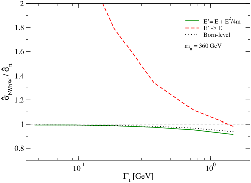
Figure 4: Ratios of the partonic cross sections for $gg\to bW^{+}\bar{b}W^{-}$ and $gg\to t\bar{t}$, in the color-singlet channel at ${{m}_{t\bar{t}}}=360$ GeV. These are plotted as functions of $\Gamma_{t}$. Green solid, red dashed and black dotted lines are those with the modified energy $E^{\prime}$, with $E$ instead of $E^{\prime}$, and for the Born cross-sections, respectively.

We confirm that the ratio approaches to unity as $\Gamma_{t}$ is reduced, in the case that we use our relativistic formulas (green solid line) or in the case that we use the tree-level cross sections (black dotted line). In sharp contrast, the ratio does not approach to unity in the case that we replace $E^{\prime}$ by $E$ (red dashed line) due to the mismatch problem. It shows invalidity of the non-relativistic approximation far above the threshold, especially for the fully differential cross section.

As is well known, the leading-order bound-state effects in the $t\bar{t}$ threshold region are contained in the $S$-wave part of the amplitude. In the case of $gg\to t\bar{t}$, the $S$-wave contributions reside in the $J=0$ amplitude both for the color-singlet and color-octet channels. Hence, it may be more appropriate to include the bound-state effects only in the $J=0$ amplitude, rather than multiplying the whole $t\bar{t}$ amplitude by the enhancement factor as in Eq. (8). Theoretically, the difference between the two prescriptions is subleading. We examine this feature by comparing the $t\bar{t}$ invariant-mass distributions computed in both ways.

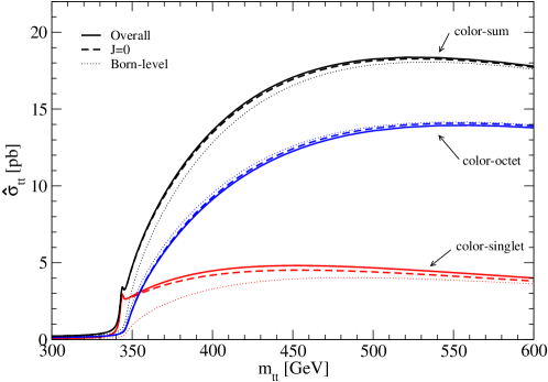
Figure 5: Partonic $t\bar{t}$ invariant-mass distributions for $gg\to t\bar{t}$ in the color-singlet (red), color-octet (blue) channels, and the sum of them (black). The solid lines are calculated by multiplying the bound-state enhancement factor to the whole $t\bar{t}$ amplitude. The dashed lines are calculated as the sum of contributions from all $J$’s, where only the $J=0$ amplitude is multiplied by the enhancement factor. The dotted lines represent the Born cross-sections corresponding to the above lines.

In Fig. 5, we plot the $t\bar{t}$ invariant-mass distributions for $gg\to t\bar{t}$ process. Each solid line represents the cross section computed using Eq. (10), namely, the whole Born cross-section (the sum of the Born cross-sections for all $J$’s) is multiplied by the enhancement factor. Each dashed line represents the sum of the cross sections for all $J$’s, where only the $J=0$ cross section is multiplied by the enhancement factor. The red (solid and dashed) lines represent the cross sections for $gg\to t\bar{t}$ in the color-singlet channel, while the blue (solid and dashed) line represent those in the color-octet channel.

The cross section in the singlet channel is more enhanced if we use the overall prescription, Eq. (10), since the force between the color-singlet $t\bar{t}$ pair is attractive and hence the enhancement factor is larger than one. The difference of the two prescriptions is sizable only above the $t\bar{t}$ threshold and becomes maximal around $m_{t\bar{t}}\simeq 400$ GeV, where the difference is about 7%. On the other hand, the cross section in the octet channel is more reduced if we use the overall prescription, since the force between the color-octet $t\bar{t}$ pair is repulsive and the enhancement factor is (slightly) less than one. The difference of the two prescriptions is at most 2%. The black lines (solid and dashed) represent the sum of the cross sections for $gg\to t\bar{t}$ in the above two channels. The difference of the two prescriptions in this case is at most about 1%, since the differences have opposite signs in the two channels and are largely canceled. Thus, the difference of the two prescriptions is rather small and much smaller than other subleading corrections which we neglect in our analysis. Furthermore, we have checked that the above tendencies are not changed significantly by the ISR effects. Therefore, for simplicity of our analysis, we will adopt the overall prescription in the following analysis, namely, we will not decompose the amplitude into different $J$’s.

In the case of $q\bar{q}\to t\bar{t}$, there is only the $J=1$ color-octet channel at tree level. Hence, the enhancement factor multiplies the whole amplitude also in this case.

2.2 Effects of large $\Gamma_{t}$

In this subsection we describe how we incorporate part of the subleading corrections that are induced by the large top-quark width. As an inevitable consequence of numerically integrating the fully differential cross sections for $I\to t\bar{t}\to bW^{+}\bar{b}W^{-}$, there is a significant phase-space-suppression effect. We partly compensate this effect, which is related to a gauge cancellation inherent in the inclusive cross section.

First, we briefly review existing theoretical studies on the treatment of the top-quark width, in the cases with and without bound-state effects. In the latter case, many schemes have been proposed for incorporating the top-quark width. The use of the top-quark propagator in Eq. (2) is called the fixed-width scheme (FWS). It is widely used in simple analysis of the cross sections which include the top quark as an unstable intermediate particle. It is known, however, that subleading electroweak effects are not properly treated in this scheme. At present, the complex-mass scheme (CMS) [39] seems to be most advanced from a practical point of view, due to the simplicity of its implementation. In fact, for the process $e^{+}e^{-}\to W^{+}W^{-}$, which is kinematically similar to $t\bar{t}$ productions, the fully differential cross section has been computed incorporating the effects of $W$-boson width with NLO accuracy in this scheme, basically in all kinematical regions [40]. For $t\bar{t}$ productions in hadron collisions, the fully differential cross sections is computed incorporating top-quark width with LO accuracy in CMS, and various differential cross sections in different schemes were compared [30]. In particular, the study has shown an agreement within errors between all the calculated cross sections in CMS and in FWS. (FWS is simpler but less sophisticated than CMS.)

Regarding $t\bar{t}$ productions in the threshold region including the bound-state effects, studies on the finite-width effects are most advanced in the total cross section for $e^{+}e^{-}\to t\bar{t}$. The finite-width effects have been incorporated with NNLO accuracy [41, 42], using the velocity-Non-Relativistic QCD (vNRQCD) effective field theory framework [43, 44]. Recently an NLO correction to the total cross section arising from the single-top resonance region has been pointed out and computed in [31], using unstable-particle effective field theory [45, 46]. On the other hand, in the corresponding fully differential cross section the width effects are incorporated only up to NLO accuracy [47] (apart from the contributions from the single-top resonance region). MC generators, developed specifically for simulation studies in the threshold region of the $e^{+}e^{-}\to t\bar{t}$ process, have incorporated both bound-state effects and finite-width effects in the LO approximation [22, 24]. For $t\bar{t}$ productions in hadron collisions, only the $t\bar{t}$ invariant-mass distributions have been computed with NLO accuracy, incorporating the bound-state effects, finite-width effects and ISR effects in the threshold region [20, 21].

One effect is known to be particularly important in computing the fully differential cross sections in the threshold region of $t\bar{t}$ productions. It is the phase-space-suppression effect [25, 26, 48], which is formally an NNLO effect of the top-quark width, but it seriously modifies the shape of the sharply rising $S$-wave cross section as a function of $m_{t\bar{t}}$, after integrating the differential cross section over the final-state phase-space [25]. Let us briefly explain this effect. The $t\bar{t}$ cross section starts to rise below the $t\bar{t}$ threshold $m_{t\bar{t}}=2m_{t}$ as a result of formation of $t\bar{t}$ resonances. This means that the dominant kinematical configuration is such that one of $t$ and $\bar{t}$ is on-shell and the other is off-shell. Therefore, the phase-space of $bW$ which decayed from the off-shell $t$ or $\bar{t}$ is reduced as compared to the on-shell case. This suppresses the production cross section, and this effect is automatically incorporated if we integrate the LO differential cross section numerically over the phase-space of the final $bW^{+}\bar{b}W^{-}$. A remarkable feature is that there is another effect at NNLO which exactly cancels the phase-space-suppression effect, for the integrated cross section at each $t\bar{t}$ invariant-mass [49, 50]. This is the Coulomb-enhancement effect due to gluon exchanges between $t$ and $\bar{b}$ (decayed from $\bar{t}$) and between $\bar{t}$ and $b$. The cancellation is guaranteed by gauge invariance (Ward identity). It protects the $t\bar{t}$ resonance widths from being determined by gauge-dependent off-shell width of the top quark. Consequently the only surviving NNLO effect to the $t\bar{t}$ resonance widths turns out to be the time-dilatation effect due to the relative motion of $t$ and $\bar{t}$ inside the resonances, which is gauge independent.

Thus, we face a problem when we compute differential cross sections in the $t\bar{t}$ threshold region by a MC generator: The phase-space-suppression effect is automatically incorporated, while the Coulomb-enhancement effect due to gluon exchanges between $t$ and $\bar{b}$ (or $\bar{t}$ and $b$) is difficult to incorporate in a MC generator. (This is not yet achieved even in theoretical computations of the $e^{+}e^{-}\to t\bar{t}$ differential cross sections.) Our prescription in this study is only effective. Since we know that the phase-space-suppression effect is canceled in the inclusive $t\bar{t}$ cross section, we multiply the $t\bar{t}$ amplitude ${\cal M}^{(c)}_{t\bar{t}}(I\to t\bar{t}\to bW^{+}\bar{b}W^{-})$ by an enhancement factor such that the phase-space-suppression factor is canceled. In addition, we include the non-resonant diagrams, which are formally ${\cal O}(\Gamma_{t}/m_{t})$ compared to the LO amplitude.

Hence, our full amplitude at the parton level is given by

$${\cal M}_{bW^{+}\bar{b}W^{-}}^{(c)}(I\to bW^{+}\bar{b}W^{-})=\widetilde{{\cal M}}_{t\bar{t}}^{(c)}+\widetilde{{\cal M}}^{(c)}_{\rm nr}$$ (22)

with

$$\widetilde{{\cal M}}^{(c)}_{t\bar{t}}={\cal M}^{(c)}_{t\bar{t}}\times\left[\frac{m_{t}\Gamma_{t}}{\sqrt{s_{t}}\Gamma_{t}(s_{t})}\cdot\frac{m_{t}\Gamma_{t}}{\sqrt{s_{\bar{t}}}\Gamma_{t}(s_{\bar{t}})}\right]^{\frac{1}{2}},$$ (23)

$$\widetilde{{\cal M}}^{(c)}_{\rm nr}={\cal M}^{(c)}_{t\bar{t},{\rm tree}}\times\left(1-\left[\frac{m_{t}\Gamma_{t}}{\sqrt{s_{t}}\Gamma_{t}(s_{t})}\cdot\frac{m_{t}\Gamma_{t}}{\sqrt{s_{\bar{t}}}\Gamma_{t}(s_{\bar{t}})}\right]^{\frac{1}{2}}\right)+{\cal M}_{\rm nr}^{(c)}\,,$$ (24)

where ${\cal M}^{(c)}_{t\bar{t}}$ is defined by Eqs. (8) and (9), and ${\cal M}^{(c)}_{\rm nr}$ denotes the sum of the tree-level non-resonant diagrams. The factor in the square bracket represents the inverse of the phase-space-suppression factor (see App. B for the derivation), where $\Gamma_{t}(s_{t})$ denotes the running top-quark width in unitary gauge evaluated at the top-quark invariant-mass $s_{t}$; its explicit form is given in App. B, Eq. (43). At large $t\bar{t}$ invariant-masses, the bound-state effects diminish, namely ${{\cal M}}^{(c)}_{t\bar{t}}\to{\cal M}^{(c)}_{t\bar{t},{\rm tree}}$, hence the above $bW^{+}\bar{b}W^{-}$ amplitude is defined such that it reduces to the tree-level amplitude, ${\cal M}_{bW^{+}\bar{b}W^{-}}^{(c)}\to{\cal M}^{(c)}_{t\bar{t},{\rm tree}}+{\cal M}_{\rm nr}^{(c)}$.

At the differential level, the above treatment of the cancellation of the phase-space-suppression effect is only effective, since the Coulomb-enhancement effect does not cancel the phase-space-suppression effect at each kinematical point. Nevertheless, we consider that a higher priority should be given to the gauge cancellation mechanism that is inherent in the inclusive cross section. We also note that the replacement $E\to E^{\prime}$ in the Green function, Eqs. (8) and (9), automatically incorporates the time-dilatation effects to the resonance widths.

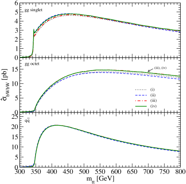
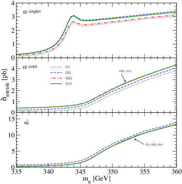
Figure 6: Partonic $t\bar{t}$ invariant-mass distributions for $gg\to t\bar{t}$ and $q\bar{q}\to t\bar{t}$ in the individual channels. Four lines in each figure are computed from (i) $|{\cal M}^{(c)}_{t\bar{t}}|^{2}$ (black dotted), (ii) $|\widetilde{{\cal M}}^{(c)}_{t\bar{t}}|^{2}$ (blue dashed), (iii) $|{\cal M}^{(c)}_{t\bar{t}}+{\cal M}^{(c)}_{\rm nr}|^{2}$ (red dot-dashed), and (iv) $|\widetilde{{\cal M}}^{(c)}_{t\bar{t}}+\widetilde{{\cal M}}^{(c)}_{\rm nr}|^{2}$ (green solid). The figures in the right show the magnification of the threshold region.

In Fig. 6, we compare the $t\bar{t}$ invariant-mass distributions for $gg\to t\bar{t}$ and $q\bar{q}\to t\bar{t}$ in all the channels, which are computed by integrating the following four cross sections over the $bW^{+}\bar{b}W^{-}$ phase-space, where the $t\bar{t}$ invariant-mass $m_{t\bar{t}}$ is defined as the invariant-mass of the final $bW^{+}\bar{b}W^{-}$ system: (i) $|{\cal M}^{(c)}_{t\bar{t}}|^{2}$ (black dotted), (ii) $|\widetilde{{\cal M}}^{(c)}_{t\bar{t}}|^{2}$ (blue dashed), (iii) $|{\cal M}^{(c)}_{t\bar{t}}+{\cal M}^{(c)}_{\rm nr}|^{2}$ (red dot-dashed), and (iv) the absolute square of our formula Eq. (22) (green solid). Comparing the distributions for (i) and (ii), or, (iii) and (iv), we see that the phase-space-suppression effects are sizable especially close to the threshold of $gg\to t\bar{t}$ in the color-singlet channel. This is consistent with the explanation given above. In particular, in each figure the difference between (iii) and (iv) is hardly visible at large $m_{t\bar{t}}$. We may also compare the distributions for (i) and (iii), or, (ii) and (iv), to see the contributions of the non-resonant amplitude. The contributions become comparatively larger at high energies for gluon-fusion channels, since the contribution of the $s$-channel diagram in ${\cal M}^{(c)}_{t\bar{t}}$ decreases, while contributions of the single-resonant diagrams in ${\cal M}^{(c)}_{\rm nr}$ increase. On the other hand, for $q\bar{q}$ channel, contributions from the non-resonant diagrams are small everywhere.

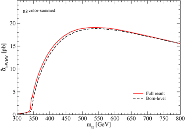
(a)	(b)

Figure 7: $t\bar{t}$ invariant-mass distributions for the processes $gg\to bW^{+}\bar{b}W^{-}$ (color-summed) and $q\bar{q}\to bW^{+}\bar{b}W^{-}$. The red solid line is plotted using Eq. (22) for the partonic amplitude, while the black dashed line represents the Born-level cross section.

In Fig. 7(a) we plot the $t\bar{t}$ invariant-mass distributions for $gg\to bW^{+}\bar{b}W^{-}$ (sum of the color-singlet and octet channels), using Eq. (22) after integrating over the $bW^{+}\bar{b}W^{-}$ phase-space (red solid line). The $t\bar{t}$ invariant-mass distribution at the Born level for $gg\to bW^{+}\bar{b}W^{-}$ in FWS is also plotted (black dashed line). The difference of the two lines signifies the bound-state effects, after including the non-resonant diagrams and compensating the phase-space-suppression effect. The enhancement of the distribution by the bound-state effect is visible not only in the threshold region but also up to about $m_{t\bar{t}}=500$ GeV. The enhancement factors are about 1.05 and 1.02 at $m_{t\bar{t}}=400$ GeV and 500 GeV, respectively. The $t\bar{t}$ invariant-mass distributions for $q\bar{q}\to bW^{+}\bar{b}W^{-}$ are also plotted in Fig. 7(b). The enhancement factor is smaller than unity because of the repulsive force, whose values are about 0.96 and 0.98 at $m_{t\bar{t}}=400$ GeV and 500 GeV, respectively.

2.3 Inclusion of ISR effects and $K$-factors

In this subsection we explain how we incorporate the ISR effects in the cross sections in our framework. In addition, we determine the $K$-factors to match our predictions for the $t\bar{t}$ invariant-mass distributions to the available NLO predictions.

In hadron collisions, it is important to include the ISR effects. In our framework, they are incorporated by connecting the differential cross sections computed from the matrix elements Eq. (8) to a parton-shower simulator such as PYTHIA [51] or HERWIG [52]. In addition, we include “$K$-factors” as the normalization constants of the cross sections for $I\to bW^{+}\bar{b}W^{-}$ in the individual channels. The $K$-factors are determined such that the $t\bar{t}$ invariant-mass distribution for each channel in the threshold region matches the corresponding NLO prediction in the threshold region. We also extrapolate these $K$-factors to the large $m_{t\bar{t}}$ region. The main reason to do so is a lack of the NLO predictions in the large $m_{t\bar{t}}$ region for the individual channels: The present theoretical prediction for the NLO $t\bar{t}$ invariant-mass distribution in the large $m_{t\bar{t}}$ region is provided numerically only for the color-summed cross section for on-shell top-quark productions [12]. Theoretically, by naive extrapolation of the $K$-factors, we reproduce the double-logarithmic terms of the cross sections correctly in the large $m_{t\bar{t}}$ region, due to the universal structure of soft-gluon emissions; on the other hand, we do not reproduce the single-logarithmic and non-logarithmic terms.

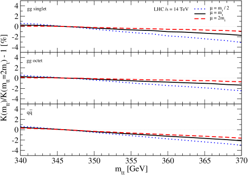
Figure 8: $m_{t\bar{t}}$ dependence of the $K$-factors for $t\bar{t}$ production in $gg$ color-singlet (top), color-octet (middle) and $q\bar{q}$ (bottom) channels at the LHC $\sqrt{s}=14$ TeV. The dashed, solid and dotted lines are obtained with $\mu_{R}=\mu_{F}=\kappa m_{t}$ with $\kappa=0.5$, 1 and 2, respectively.

The NLO corrections to the $t\bar{t}$ invariant-mass distributions in the threshold region are known for the individual channels [20, 21]. The corrections are given in terms of the hard-correction factors and the gluon radiation functions. The major difference of the predictions of [20] and [21] is that in the latter predictions contributions from high $\sqrt{\hat{s}}$ (the c.m. collision energy of the initial partons) are included more accurately. Hence, we use the latter predictions to compute the $K$-factors. We can determine the $K$-factors by taking the ratios of these NLO partonic cross sections and our (LO) partonic cross sections given in Sec. 2.2. Since the NLO cross sections [20, 21] do not include contributions from non-resonant diagrams ${\cal M}_{\rm nr}^{(c)}$, accordingly we incorporate only the contributions from the resonant diagrams $\widetilde{\cal M}_{t\bar{t}}^{(c)}$ in the LO cross sections when we compute the $K$-factors. (In most of the threshold region, the effect of $\widetilde{\cal M}_{\rm nr}^{(c)}$ is irrelevant in any case, since resonant diagrams dominate.) Furthermore, in calculating the $K$-factors, we use the CTEQ6M PDFs [56] and the 2-loop running of the strong coupling constant $\alpha_{s}$ for the NLO $m_{t\bar{t}}$ distribution, while the CTEQ6L1 PDFs and the 1-loop running of $\alpha_{s}$ are used for the LO distribution. (We find that the $K$-factors obtained by using the MSTW2008 PDFs [57] are quite similar.)

In general, the $K$-factors depend on $m_{t\bar{t}}$. We first examine $m_{t\bar{t}}$-dependences of the $K$-factors as we choose different renormalization and factorization scales, $\mu_{R}$ and $\mu_{F}$. The renormalization scale $\mu_{R}$ enters the NLO formula as the scale of the strong coupling constant and also through the logarithmic term in the hard-vertex function; see Eq. (3.2) of [21]. On the other hand, the factorization scale $\mu_{F}$ enters the NLO formula as the scale of the parton distribution functions (PDFs) and through the terms with $\ln\left(m_{t\bar{t}}^{2}/\mu_{F}^{2}\right)$ in the gluon radiation functions; see Eqs. (3.4-3.7) of [21]. We find that, the $m_{t\bar{t}}$-dependences of the $K$-factors can be relatively flat in the threshold region, with appropriate choices of $\mu_{R}$ and $\mu_{F}$. In this case, extrapolation of the $K$-factors from the threshold region to the high $m_{t\bar{t}}$ region can be performed trivially. Indeed, for simplicity of our analysis, we take the $K$-factors to be independent of $m_{t\bar{t}}$. In Fig. 8, we plot the $K$-factors of the $t\bar{t}$ invariant-mass distributions in the individual channels at the LHC with $\sqrt{s}=14$ TeV, in the cases that we choose the scales as $\mu_{R}=\mu_{F}=\kappa m_{t}$ with $\kappa=0.5,1,2$. As can be seen, the $m_{t\bar{t}}$-dependence of the $K$-factors are mild. We have also examined the $K$-factors corresponding to the LHC with $\sqrt{s}=7$ TeV and Tevatron with $\sqrt{s}=1.96$ TeV; we find that the $K$-factors are only mildly dependent on $m_{t\bar{t}}$ also in these cases. In Table 1, we list the numerical values of the $K$-factors for all the channels corresponding to the LHC $\sqrt{s}=14$ TeV, 7 TeV and Tevatron $\sqrt{s}=1.96$ TeV, obtained at $m_{t\bar{t}}=2m_{t}$ for $\mu_{R}=\mu_{F}=\kappa m_{t}$ with $\kappa=0.5$, 1, 2. The values of the $K$-factors for $\kappa=1$ will be used in the following.

	LHC 14 TeV			LHC 7 TeV			Tevatron
$\kappa$	$gg^{[c=1]}$	$gg^{[c=8]}$	$q\bar{q}$	$gg^{[c=1]}$	$gg^{[c=8]}$	$q\bar{q}$	$gg^{[c=1]}$	$gg^{[c=8]}$	$q\bar{q}$
0.5	0.79	1.02	0.88	0.87	1.13	0.89	1.30	1.72	0.87
1	1.14	1.39	1.16	1.31	1.60	1.18	2.11	2.60	1.18
2	1.48	1.75	1.42	1.75	2.07	1.45	2.95	3.48	1.45

Table 1: $K$-factor normalization constant for each channel ($gg$ color-singlet, octet and $q\bar{q}$) for the LHC $\sqrt{s}=14$ TeV, 7 TeV and the Tevatron, with setting the factorization and renormalization scales to $\mu_{R}=\mu_{F}=\kappa m_{t}$ with $\kappa=0.5$, 1, 2.

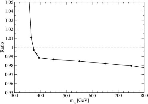
Figure 9: Ratio of the two color-summed $t\bar{t}$ invariant-mass distributions: The former is our prediction including the $K$-factors but omitting the non-resonant diagrams, and the latter is the NLO prediction by MC@NLO for on-shell top quarks.

We check consistency of our $K$-factor normalization in the large $m_{t\bar{t}}$ region, by comparing our prediction for the color-summed $t\bar{t}$ invariant-mass distribution with the NLO prediction. In Fig. 9 we plot the ratio of these two cross sections. In the former distribution, we include the $K$-factors, while we do not include the non-resonant diagrams $\widetilde{\cal M}_{\rm nr}^{(c)}$ [c.f. (ii) of Fig. 6]. The latter distribution is computed for the on-shell $t\bar{t}$ productions, by MC@NLO [34, 35] with CTEQ6M PDFs with a scale choice $\mu_{F}=\mu_{R}=\sqrt{m_{t}^{2}+p_{T,t}^{2}}$. As can be seen, both cross sections are mutually consistent within 2% accuracy up to $m_{t\bar{t}}=800$ GeV.

Including non-resonant diagrams in a way that the gauge cancellation holds effectively, our final formula for the matrix element at parton level reads

$${\cal M}_{bW^{+}\bar{b}W^{-}}^{(c)}(I\to bW^{+}\bar{b}W^{-})=\sqrt{K}\,\left[\widetilde{{\cal M}}_{t\bar{t}}^{(c)}+\widetilde{{\cal M}}^{(c)}_{\rm nr}\right].$$ (25)

$\widetilde{{\cal M}}_{t\bar{t}}^{(c)}$ and $\widetilde{{\cal M}}^{(c)}_{\rm nr}$ are given in Eqs. (23) and (24).

3 Event Generation and Top-Quark Distributions

In this section, we present numerical evaluations of various kinematical distributions of the top-quark computed from the $pp\to bW^{+}\bar{b}W^{-}$ cross section, using the theoretical framework explained in the previous section. In particular we study the bound-state effects on these distributions.

Our numerical calculations are carried out based on the MadGraph output [58] which makes use of the HELAS subroutines [59] for helicity-amplitude calculations. The original MadGraph output code has been modified to implement the color-decomposition and to include the bound-state effects via the Green functions. For the convenience of the readers, we collect the formulas necessary for decomposing amplitudes into the color-singlet and octet components of the $t\bar{t}$ (or $b\bar{b}$) system in Appendix C. In particular, we discuss how to implement the color decomposition into the MadGraph notation. The bound-state correction factor

$${\cal G}^{(c)}(E,\vec{p})=\frac{G^{(c)}(E,\vec{p})}{G_{0}(E,\vec{p})},$$ (26)

c.f. Eq. (8), is pre-tabulated to save time for computing the momentum-space Green functions.

We perform phase-space integrations using BASES/SPRING [60], or alternatively by adapting our code to MadEvent [32, 33] utilities (ver. 4.4.42), where both tools are able to generate unweighted events at the partonic final-state level. For each event, we assign the specific color-flow according to an ordinary manner, except the color-singlet channel, as explained in Appendix C. The generated events can be subsequently provided e.g. to PYTHIA for simulations of parton-showering and hadronizations.

In the main body of this paper, we do not consider the decay of $W$’s but consider only the observables constructed from the $bW^{+}\bar{b}W^{-}$ final state. The $W$-boson decays can be incorporated at the PYTHIA stage, where however the polarization of $W$-bosons cannot be taken into account. Alternatively, one can calculate the helicity amplitudes including the decay of $W$-bosons by specifying a decay mode for each $W$-boson. In Appendix D, as a sample case, we examine the distributions of dileptons in the dilepton mode, where both $W$’s decay leptonically, and study the effects of $W$-boson polarization and bound-state corrections.

Below we show the results at the partonic $bW^{+}\bar{b}W^{-}$ final-state level. We do not discuss the parton-showering and hadronization effects, in order to concentrate on the examination of bound-state effects. For the parton distribution functions, we use the CTEQ6L1 parameterization with the LO evolution (1-loop running) of the QCD coupling constant. We set the renormalization and factorization scales to $\mu_{R}=\mu_{F}=m_{t}$ and incorporate the $K$-factors obtained in Sec. 2.3 to the cross sections in the individual channels. [The final formula for the matrix element is given by Eq. (25).] We set the top-quark pole-mass, the (tree-level) on-shell top-quark width and the strong coupling constant as $m_{t}=173$ GeV, $\Gamma_{t}=1.49$ GeV and $\alpha_{s}(M_{z})=0.1298$, respectively.

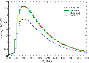
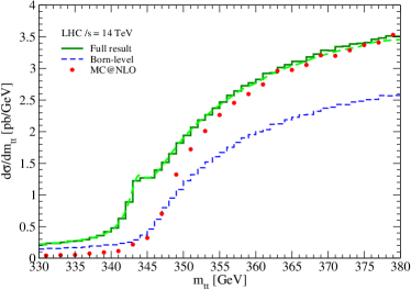
(a)                                                            (b)

Figure 10: $t\bar{t}$ invariant-mass distribution in $pp\to bW^{+}\bar{b}W^{-}$ at $\sqrt{s}=14$ TeV. Green solid line is our full prediction and blue dashed line is the Born-level prediction. The NLO $t\bar{t}$ production computed by MC@NLO is also plotted in red dots. Right figure is the magnification of the threshold region.

In Fig. 10(a), we plot the $t\bar{t}$ invariant-mass distribution in $pp\to bW^{+}\bar{b}W^{-}$ production at $\sqrt{s}=14$ TeV. The $t\bar{t}$ invariant-mass $m_{t\bar{t}}$ is defined as the invariant-mass of the final $bW^{+}\bar{b}W^{-}$ system. The green solid line represents the full result which includes the bound-state effects as well as the $K$-factors, and the blue dashed line represents the Born-level result (the LO prediction in the conventional perturbative QCD approach). Fig. 10(b) shows a magnification of the same cross sections in the threshold region. As shown in [20, 21], theoretically the bound-state effects can be seen most clearly in the shape of the $m_{t\bar{t}}$ distribution in the threshold region. One can see that the cross section is enhanced over the Born cross-section significantly by the bound-state effects, and there appears a broad peak below the threshold corresponding to the ${}^{1}S_{0}$ resonance state in the color-singlet $t\bar{t}$ channel. Far above the threshold, the bound-state effects disappear and the cross section approaches the Born-level distributions, up to the $K$-factor normalization.

In the same figures, we also compare our prediction with the NLO $m_{t\bar{t}}$ distribution computed by MC@NLO [34, 35] with CTEQ6M PDFs and the scale choice of $\mu_{F}=\mu_{R}=\sqrt{m_{t}^{2}+p_{T,t}^{2}}$. The latter prediction includes the full NLO QCD corrections (but not the Coulomb resummation) for the on-shell $t\bar{t}$ productions; we switched on an option of MC@NLO to incorporate off-shellness of the top-quarks effectively by re-weighting the cross section by skewed Breit-Wigner functions [61], so that the cross section is non-zero below the threshold. (However, non-resonant diagrams are not incorporated.) Below and near the threshold, our prediction is much larger than the MC@NLO prediction, due to the bound-state formation. The two cross sections become approximately equal from around $m_{t\bar{t}}\sim 370$–380 GeV up to larger $m_{t\bar{t}}$. Note that, in Fig. 9, the contributions from non-resonant diagrams are not included in our full prediction, whereas in Figs. 10 they are included. Integrating the distributions over $m_{t\bar{t}}$, the total cross section by our full (Born-level) calculation is estimated as $\sigma_{bW^{+}\bar{b}W^{-}}=855$ pb (633 pb), while we obtain $\sigma_{t\bar{t}}=816$ pb as the MC@NLO prediction.

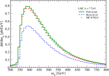
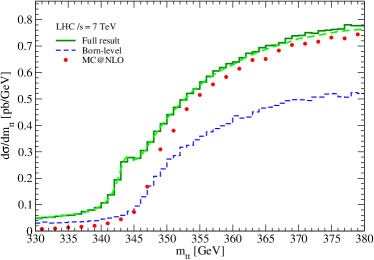
Figure 11: The same as Fig. 10, but for the LHC $\sqrt{s}=7$ TeV.

The shape of the $m_{t\bar{t}}$ distribution at the LHC 7 TeV, shown in Fig. 11, is similar to that for the LHC 14 TeV. The total cross sections are estimated to be 158 pb, 106 pb and 146 pb by our full, Born-level calculations and MC@NLO, respectively.

Let us examine other distributions of the top quark. From Figs. 10 and 11, it is obvious that the phase-space region, where the bound-state effects are important, corresponds to a rather limited portion of the full top-quark events produced at the LHC. Thus, in various distributions formed by the full events, the bound-state effects may well be negligible in practice. In order to examine the bound-state effects closely, in the following we consider the events restricted by $m_{t\bar{t}}\leq 370$ GeV (except where otherwise stated), instead of considering the full events. They amount to about 9% (8%) of the full events according to our calculation with (without) the bound-state corrections at the LHC $14$ TeV. Due to the large $t\bar{t}$ cross sections at the LHC, still a large number of such near-threshold events would be accumulated. In this paper, we do not discuss the important subject of how to measure $m_{t\bar{t}}$ in real experiments, which requires detailed studies of errors and fake solutions; one may find them in earlier studies [15, 17].

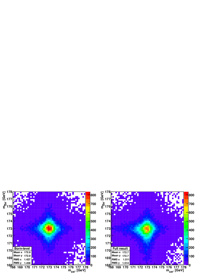
(a)                                                            (b)

Figure 12: Two-dimensional density plots of the $bW^{+}$ and $\bar{b}W^{-}$ invariant-masses, for the events with $m_{t\bar{t}}\leq 370$ GeV at the LHC $\sqrt{s}=14$ TeV. Left figure (a) is the Born-level prediction and right figure (b) is our full result (including the bound-state corrections and $K$-factors). The mean value and the root-mean-square value displayed in each figure are calculated for the events within the frame of the figure.

One observes a characteristic bound-state effect in the $(bW^{+})$-$(\bar{b}W^{-})$ double-invariant-mass distribution. In Figs. 12, we show the density plots of the invariant-masses of the $bW^{+}$ and $\bar{b}W^{-}$ systems, given by (a) the Born-level prediction and (b) our full prediction. In each figure, the number of events is normalized to 100,000 in total, and the number of events per bin (0.2 GeV$\times$0.2 GeV) is plotted with graded colors. The Born-level prediction (a) is essentially determined by the product of the Breit-Wigner functions, hence the distribution is almost reflection symmetric with respect to the on-shell lines $(p_{b}+p_{W^{+}})^{2}=m_{t}^{2}$ and $(p_{\bar{b}}+p_{W^{-}})^{2}=m_{t}^{2}$. By contrast, the distribution by our full prediction (b) is not symmetric and biased towards the configuration, where one of $t$ or $\bar{t}$ is on-shell and the other has an invariant-mass smaller than $m_{t}$. In fact, such a configuration is known to be the dominant configuration just below the threshold in $e^{+}e^{-}\to t\bar{t}$ [25, 24], although in that case deviation from the double Breit-Wigner distribution [Fig. 12(a)] is more prominent. (Note that, below the threshold, $t$ and $\bar{t}$ cannot become simultaneously on-shell.)

In order to quantify the correlated deformation of the double-invariant-mass distribution, we count the fraction of the events for which both or either of the $bW^{+}$ and $\bar{b}W^{-}$ invariant-masses satisfy

$$|m_{bW}-m_{t}|\leq k\Gamma_{t},$$ (27)

where $k=1,2,\dots,5$. These fractions are tabulated in Table 2 for our full prediction and for the Born-level prediction. The bound-state effect reduces the fraction for which both invariant-masses are close to on-shell more than the fraction for which either of the invariant-masses is close to on-shell. In the former case, the change of the fraction by the bound-state effect amounts up to about 4%. For comparison, we also tabulate the same fractions for the full events; in this case, the variation of the fractions are small and at most 1%. In any case, a proper understanding of this effect would be important, since it potentially biases the mass cut and may affect, for instance, the top-quark mass measurement with high accuracy.

	$m_{t\bar{t}}\leq 370$ GeV		Full events
$k$	both [%]	either [%]	both [%]	either [%]
1	37.0 (41.1)	87.0 (87.6)	46.8 (47.7)	90.3 (90.4)
2	55.5 (59.0)	95.2 (95.2)	67.6 (68.3)	97.0 (97.0)
3	64.2 (66.3)	97.3 (97.1)	76.3 (76.8)	98.5 (98.5)
4	69.2 (70.3)	98.1 (98.0)	81.0 (81.4)	99.1 (99.1)
5	72.3 (72.9)	98.6 (98.4)	83.9 (84.2)	99.4 (99.4)

Table 2: A fraction of events which satisfy $|m_{bW}-m_{t}|\leq k\Gamma_{t}$ for both or either of the $bW$ invariant-masses. The events with $m_{t\bar{t}}\leq 370$ GeV as well as the full events at the LHC 14 TeV are considered. In the bracket is shown the result in Born-level.

Let us explain the mechanism how the bound-state effects alter the double-invariant-mass distribution. As shown in Appendix A, the leading part of the $t\bar{t}$ amplitude ${\cal M}^{(c)}_{t\bar{t}}$ has a form

$${\cal M}^{(c)}_{t\bar{t}}\propto\left\langle\frac{1}{m_{t\bar{t}}-[2\sqrt{\hat{p}^{2}+m_{t}^{2}}+V_{\rm QCD}^{(c)}(r)]}\right\rangle\,$$

$$~{}~{}~{}~{}~{}~{}~{}~{}~{}~{}~{}~{}~{}~{}~{}~{}~{}\times\left(\frac{1}{\hat{p}_{t}^{0}-\sqrt{\hat{p}^{2}+m_{t}^{2}}}+\frac{1}{\hat{p}_{\bar{t}}^{0}-\sqrt{\hat{p}^{2}+m_{t}^{2}}}\right)\,$$ (28)

where $\hat{p}_{t}^{\mu}\equiv\hat{p}_{b}^{\mu}+\hat{p}_{W^{+}}^{\mu}$ and $\hat{p}_{\bar{t}}^{\mu}\equiv\hat{p}_{\bar{b}}^{\mu}+\hat{p}_{W^{-}}^{\mu}$ are defined in the $t\bar{t}$ c.m. frame, and $\hat{p}\equiv|\vec{\hat{p}}_{t}|$ denotes the magnitude of the top-quark three-momentum in this frame. The first factor on the right-hand side $\langle(m_{t\bar{t}}-H)^{-1}\rangle$, with $H=2\sqrt{\hat{p}^{2}+m_{t}^{2}}+V_{\rm QCD}^{(c)}(r)$ [c.f. Eq. (15)], denotes the Green function of the $t\bar{t}$ system. We suppress the top-quark width for simplicity. In the case that $t\bar{t}$ is in the singlet channel ($c=1$), the potential energy between $t$ and $\bar{t}$ is negative, $V_{\rm QCD}^{(1)}(r)<0$. Therefore, the denominator of the Green function become close to zero (hence, the Green function is most enhanced) if $\hat{p}$ is somewhat larger than the on-shell momentum $p_{\rm OS}\equiv\sqrt{{m_{t\bar{t}}^{2}}/{4}-m_{t}^{2}}$, i.e., $\hat{p}>p_{\rm OS}$. On the other hand, the second factor $({p_{t}^{0}-\sqrt{\hat{p}^{2}+m_{t}^{2}}})^{-1}+({p_{\bar{t}}^{0}-\sqrt{\hat{p}^{2}+m_{t}^{2}}})^{-1}$ is most enhanced when $\hat{p}=p_{\rm OS}$, since $p_{t}^{0}+p_{\bar{t}}^{0}=m_{t\bar{t}}$. Thus, there is a competition between the two factors on the right-hand side of Eq. (28). As a consequence, the dominant configuration is the one in which neither of the two factors are maximal. In fact, in the dominant configuration one of $t$ and $\bar{t}$ is on-shell and the other is off-shell: $\hat{p}_{t}^{2}=m_{t}^{2}$, $\hat{p}_{\bar{t}}^{2}<m_{t}^{2}$, or, $\hat{p}_{t}^{2}<m_{t}^{2}$, $\hat{p}_{\bar{t}}^{2}=m_{t}^{2}$. The effect is opposite in the case that $t\bar{t}$ is in the octet channel ($c=8$). Since the magnitude of the octet potential is much smaller than the singlet potential, $V_{\rm QCD}^{(8)}/V_{\rm QCD}^{(1)}=-1/8$, the bound-state effect turns out to be much larger in the singlet channel than in the octet channel.

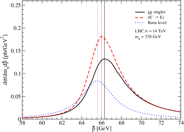
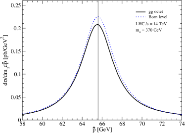
(a)                                                           (b)

Figure 13: Top-quark momentum ($\hat{p}\equiv|\vec{\hat{p}}_{t}|$) distributions in the partonic center-of-mass frame for a fixed $m_{t\bar{t}}=370$ GeV, (a) for the color-singlet channel, and (b) for the octet channel. The solid lines represent our full prediction, after omitting the non-resonant diagrams. The dotted lines represent corresponding distributions at the Born-level. In Fig. (a), the distribution by the non-relativistic formula (replacing $E^{\prime}\to E$ in the Green function) is also plotted (the red dashed line).

Displayed in Figs. 13(a) and (b) are the top-quark momentum ($\hat{p}$) distributions of the events with $m_{t\bar{t}}=370$ GeV (not with $m_{t\bar{t}}\leq 370$ GeV), for the color-singlet and octet channels, respectively. To see essential features, only the $t\bar{t}$ diagrams are taken into account and the $K$-factors are not included. In each figure, the black solid (blue dotted) line shows our full prediction (Born-level prediction). The peak momentum for each distribution is shown with a vertical line. The peak momenta of the Born-level distributions are (to a good approximation) the on-shell momentum, $\hat{p}_{\rm peak}\approx p_{\rm OS}=65.5$ GeV. We see that the bound-state effects shift the peak momentum by about 0.7 GeV to a larger value for the color-singlet distribution, while the peak momentum of the color-octet channel is shifted only by 50 MeV to a smaller value. In the color-summed cross section, the peak momentum is shifted to a larger value. Consequently, one of the invariant-masses of the $bW^{+}$ and $\bar{b}W^{-}$ systems is reduced below $m_{t}$. The integral of this effect over the region $m_{t\bar{t}}\leq 370$ GeV can be seen in Fig. 12(b).

One may suspect that the above shifts of the invariant-masses (or the shift of the peak momentum) may be an artifact of our specific method to interpolate the $t\bar{t}$ cross sections in the threshold region and in the higher $m_{t\bar{t}}$ region. To check this, let us estimate the size of the shift of the peak momentum at $m_{t\bar{t}}=370$ GeV and compare it with the above prediction. The distance a top-quark propagates before it decays is estimated as $\gamma c\tau=m_{t\bar{t}}/(2m_{t}\Gamma_{t})=0.72~{}\mbox{GeV}^{-1}=1/(1.4~{}\mbox{GeV})$. This distance is considered to be within the range where the potential $V_{\rm QCD}^{(1)}(r)$ can be estimated perturbatively, although the 1-loop potential tends to underestimate the bound-state effect. The shift of the average momentum may be estimated by $\bigl{[}\{m_{t\bar{t}}-V_{\rm QCD}^{(1)}(\gamma c\tau)\}^{2}/4-m_{t}^{2}\bigr{]}^{1/2}-p_{\rm OS}=0.66$ GeV. Hence, the effect seen in Fig. 13(a) seems to be physical.

We note that the effect elucidated here is a kind of effect that can never be seen in perturbative QCD computations for the on-shell $t\bar{t}$ productions, such as those given in [34, 35, 36]. This is because, the effect originates from the exchange of Coulomb gluons between off-shell $t$ and on-shell $\bar{t}$ (or vice versa). Our full prediction correctly incorporates the (gauge-independent) LO off-shellness of the top quark as dictated by the exchange of Coulomb gluons, which is crucial for predicting the deformations of the top-quark momentum distribution and the double-invariant-mass distribution of the $bW^{+}$ and $\bar{b}W^{-}$ systems.

Now we are in a position to understand the origin of the abnormally large enhancement of the cross section, which we observed in Sec. 2.1, in the case that we use the non-relativistic formula for the differential cross section at large $m_{t\bar{t}}$; see the red dot-dashed line in Fig. 3. The non-relativistic formula corresponds to replacing the Hamiltonian $H=2\sqrt{\hat{p}^{2}+m_{t}^{2}}+V_{\rm QCD}^{(c)}(r)$ by $H=2m_{t}+{\hat{p}^{2}}/{m_{t}}+V_{\rm QCD}^{(c)}(r)$ in the Green function in Eq. (28). Thus, the non-relativistic formula overestimates the kinetic energy of the $t\bar{t}$ system in the large $m_{t\bar{t}}$ region, $2m_{t}+{\hat{p}^{2}}/{m_{t}}>2\sqrt{\hat{p}^{2}+m_{t}^{2}}$. For this reason, the two factors on the right-hand side of Eq. (28) can be brought close to maximal simultaneously with a nearly on-shell momentum, $\hat{p}\simeq p_{\rm OS}$, since all the denominators in this expression nearly vanish. Since the individual factors are made of pole-type functions, applying an inaccurate kinematical relation only in one of the denominators can lead to a substantial overestimate of the cross section. In Fig. 13(a) we also plot the top-quark-momentum distribution computed with the non-relativistic formula, Eq. (8) after the replacement $E^{\prime}\to E$ for the singlet channel (red dashed line). As can be seen, the peak momentum approaches the on-shell momentum and the distribution is more enhanced around the peak, compared to our full prediction.

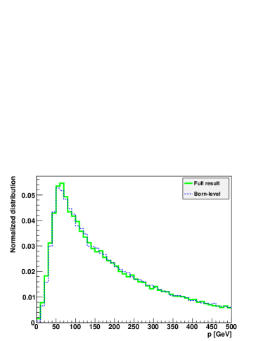
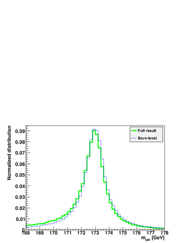
(a)                                                            (b)

Figure 14: Normalized distributions of (a) the top-quark momentum, $p=|\vec{p}_{t}|=|\vec{p}_{b}+\vec{p}_{W^{+}}|$, and (b) the $bW$ invariant-mass, both defined in the lab. frame and for the events with $m_{t\bar{t}}\leq 370$ GeV. Green solid lines represent our full predictions, while the blue dashed lines represent the Born-level predictions.

Other top-quark distributions are less affected by the bound-state effects. In Fig. 14(a), we show the normalized distribution of the top-quark momentum $p=|\vec{p}_{t}|=|\vec{p}_{b}+\vec{p}_{W^{+}}|$ in the laboratory frame. In Fig. 14(b), we show the normalized distribution of the invariant-mass of $bW$ (${bW^{+}}$ or $\bar{b}W^{-}$). The Born-level and full predictions are shown by the green solid and blue dashed lines, respectively. These lines in Fig. 14(b) correspond to the projections of Figs. 12(a,b) to the $m_{bW^{+}}$ (or $m_{\bar{b}W^{-}}$) axis. All the histograms in Figs. 14(a,b) are normalized, such that their integrals take the same value.

In $e^{+}e^{-}$ collisions, the top-quark momentum distribution in the threshold region is known to be proportional to the absolute square of the momentum-space Green function [25, 26], whose shape is strongly influenced by the bound-state effects. At hadron colliders, the top-quark momentum is boosted along the beam direction, and also the partonic collision energy is not fixed. As a result, even if we limit the events to those with $m_{t\bar{t}}\leq 370$ GeV, the distribution of the top-quark momentum ($p$, defined in the lab. frame) is not much affected by the bound-state effects at hadron colliders.

The $m_{bW}$ distribution is important for the determination of the top-quark mass, hence it should be understood well. The bound-state effects deform the Born-level $m_{bW}$ distribution towards the lower side. The mean values of $m_{bW}$ over the range $|m_{bW}-m_{t}|<5$ GeV are estimated to be 172.7 GeV and 172.9 GeV, for the full and Born-level predictions, respectively. The change of the mean value is about $-200$ MeV, for the restricted events with $m_{t\bar{t}}\leq 370$ GeV. At the LHC 7 TeV, we obtain almost the same result as in the 14 TeV case. At the Tevatron 1.96 TeV, where the $q\bar{q}$ color-octet channel dominates, the mean values of $m_{bW}$ are estimated as 172.96 GeV and 172.98 GeV, respectively. Thus, the variation of the mean value is rather small. Note that MC@NLO predicts a $m_{bW}$ distribution similar to the Born-level distribution, since it simply re-weights the on-shell $t\bar{t}$ cross-section by skewed Breit-Wigner functions.

4 Summary

In the first part of this paper (Sec. 2), we explain our theoretical framework for including the bound-state effects in the fully differential cross sections for the top-quark production and their subsequent decay processes at hadron colliders.

We formulate a theoretical basis to compute the fully differential top-quark cross-sections, which are valid at leading-order both in the threshold and high-energy regions, and which smoothly interpolate between the two regions. The tree-level $t\bar{t}$ double-resonant amplitude for each process is multiplied by a correction factor, which is written in terms of the (well-known) non-relativistic Green function, but using a modified energy. This prescription preserves the required unitarity relation between the total and differential cross sections, which would be seriously violated had we used the naive non-relativistic formula for the differential cross sections at higher energies.

We also include into the cross sections two important subleading corrections induced by the large top-quark width. (i) In addition to the $t\bar{t}$ double-resonant diagrams, which receives the above bound-state corrections, we include the contributions of non-resonant diagrams, whose effects are comparatively larger at higher energies. (This is more or less trivial.) (ii) As long as we perform numerical integrations of the differential cross sections, a sizable phase-space-suppression effect in the threshold region is inevitable, due to the sizable off-shellness of top quarks. In order to effectively account for the gauge cancellation by the Coulomb enhancement, we compensate the phase-space-suppression effect (by hand).

Finally we incorporate ISR and the $K$-factors. ISR effects are incorporated by connecting our differential cross sections to a parton-shower simulator such as PYTHIA or HERWIG. We determine the $K$-factors for the cross sections in the individual channels by matching them to the corresponding NLO $t\bar{t}$ invariant-mass distributions in the threshold region. With an appropriate choice of scales and using $m_{t\bar{t}}$-independent $K$-factors, we have checked that the color-summed $t\bar{t}$ invariant-mass distribution agrees with the conventional NLO prediction by MC@NLO reasonably well at high energies.

In the latter part of the paper (Sec. 3), using the above fully differential cross sections, we compute numerically various kinematical distributions of the top quark, constructed from the momenta of the $bW^{+}\bar{b}W^{-}$ final state (at the parton level). Our computations are carried out by MC event-generation using MadGraph, after implementing the color decomposition and the bound-state corrections to the output codes.

We confirmed that our prediction reproduces the known NLO predictions for the $t\bar{t}$ invariant-mass distribution in the threshold region (which include bound-state effects) at the LHC 7 TeV or 14 TeV; in particular it exhibits the $1S$ resonance peak below threshold. Furthermore, our prediction approaches smoothly to the conventional NLO prediction (without bound-state effects) at higher invariant-masses, from around 30 GeV above the threshold.

We restrict the events to those with $m_{t\bar{t}}\leq 370$ GeV (in the case $2m_{t}=346$ GeV), corresponding to about 10% of the full events, and examine kinematical distributions other than the $m_{t\bar{t}}$ distribution. In particular, a characteristic bound-state effect on the $(bW^{+})$-$(\bar{b}W^{-})$ double-invariant-mass distribution is observed. The distribution is deformed from the double Breit-Wigner shape, towards the configuration in which one of the $t\bar{t}$ pair is close to on-shell and the other has a smaller invariant-mass than $m_{t}$.

The effect can be understood as a consequence of a competition between the contributions from the (dominant) color-singlet Green function and from the $t$ and $\bar{t}$ propagators. If the top-quark width were tiny, the Breit-Wigner distribution would tend to a delta-function, and the top quarks would be forced to on-shell. Due to the large decay width, however, the binding effect (towards off-shell mass) and the Breit-Wigner constraint (towards on-shell mass) remain to be competitive up to a few tens GeV above the threshold. This effect lowers the mean value of each $bW$ invariant-mass by a few hundred MeV for the above restricted set of events. The correlated deformation of the double-invariant-mass distribution may affect the mass cut and eventually the top quark mass measurement at the LHC. This requires further careful investigations. It would be worth emphasizing that the bound-state effect elucidated here can never be seen in the conventional perturbative QCD corrections to the on-shell $t\bar{t}$ productions, since the off-shellness of the top quark by the LO Coulomb binding effects plays a crucial role, and therefore it signifies a unique aspect of the present study.

We examine other distributions, namely the (single) $bW$ invariant-mass distribution and top-quark-momentum distribution. The bound-state effects on these distributions as a whole are not very significant, although there are certain systematic tendencies in the small deformations of the distributions, such as the aforementioned shift of the mean value of the invariant-mass. Furthermore, the dilepton distributions are examined including the leptonic decays of $W$’s at the matrix-element level (Appendix D). We have confirmed the previous observations that the effects of $W$-boson polarization are quite significant, whereas we find that the bound-state effects are much smaller.

Appendix A Green function of the $t\bar{t}$ system

In this Appendix we explain how part of the Feynman amplitude corresponding to $I\to t\bar{t}\to bW^{+}\bar{b}W^{-}$ ($I=gg$ and $q\bar{q}$) can be identified with a Green function that dictates the time evolution of the $t\bar{t}$ system. The argument is not restricted to the non-relativistic region. In order to define the bound-state as an eigenstate of the full Hamiltonian, we consider the limit $\Gamma_{t}\to 0$.

Before providing a general argument, it would be pedagogical to demonstrate a decomposition of the three-point function $\left<{0}\,\right|T\!:\!\bar{\psi}(x)\gamma^{\mu}\psi(x)\!:\!\,\bar{\psi}(y)\,\psi(z)\left|\,{0}\,\right>$ in the free top-quark case, i.e., in the limit $\alpha_{s}\to 0$. Here, $\psi(x)$ represents the top-quark field operator. The three-point function is included, for example, in the amplitude for $\gamma^{*}\to t\bar{t}\to bW^{+}\bar{b}W^{-}$. One can express the three-point function as

$$\left<{0}\,\right|T\!:\!\bar{\psi}(x)\gamma^{\mu}\psi(x)\!:\!\,\bar{\psi}(y)\,\psi(z)\left|\,{0}\,\right>_{\rm tree}\stackrel{{\scriptstyle\rm F.T.}}{{=\!=}}\frac{{p}_{t}^{\alpha}\gamma_{\alpha}+m_{t}}{{p}_{t}^{2}-m_{t}^{2}+i\epsilon}\,\gamma^{\mu}\,\frac{-p_{\bar{t}}^{\beta}\gamma_{\beta}+m_{t}}{p_{\bar{t}}^{2}-m_{t}^{2}+i\epsilon}\rule[-19.91692pt]{0.0pt}{17.07164pt}$$ (29)

$$~{}~{}~{}~{}~{}=\Biggl{[}\frac{\Lambda_{+}(\vec{p})}{p_{t}^{0}-\omega(\vec{p})+i\epsilon}-\frac{\Lambda_{-}(\vec{p})}{{p}_{t}^{0}+\omega(\vec{p})-i\epsilon}\Biggr{]}\,\gamma^{\mu}\,\Biggl{[}\frac{\Lambda_{-}(\vec{p})}{p_{\bar{t}}^{0}-\omega(\vec{p})+i\epsilon}-\frac{\Lambda_{+}(\vec{p})}{p_{\bar{t}}^{0}+\omega(\vec{p})-i\epsilon}\Biggr{]}\,,$$

where F.T. stands for the Fourier transform, and $\omega(\vec{p})=\sqrt{\vec{p}^{\,2}+m_{t}^{2}}$. In the second equality, we have separated the contributions of particle propagating forward in time and antiparticle propagating backward in time. Here,

$$\Lambda_{\pm}(\vec{p})=\frac{\pm\omega(\vec{p})\gamma^{0}-\vec{p}\cdot\vec{\gamma}+m_{t}}{2\omega(\vec{p})}$$ (30)

represent the projection operators of a four-component spinor to the $t$ and $\bar{t}$ components. Let us drop the contributions of non-resonant parts (far off-shell contributions) in the last line of Eq. (29), which are ${\cal O}(\Gamma_{t}/m_{t})$ had we retained the top-quark width in the top quark propagator. This corresponds to taking the contribution of the time ordering $x^{0}<y^{0},z^{0}$ of the left-hand-side of the equation. Noting that $p_{t}^{0}+p_{\bar{t}}^{0}=m_{t\bar{t}}$, the resonant part can be expressed as

$$\frac{\Lambda_{-}(\vec{p})}{p_{\bar{t}}^{0}-\omega(\vec{p})+i\epsilon}\,\gamma^{\mu}\,\frac{\Lambda_{+}(\vec{p})}{p_{t}^{0}-\omega(\vec{p})+i\epsilon}\rule[-19.91692pt]{0.0pt}{17.07164pt}$$

$$~{}~{}~{}~{}~{}=\frac{\Lambda_{-}(\vec{p})\,\gamma^{\mu}\,\Lambda_{+}(\vec{p})}{m_{t\bar{t}}-2\omega(\vec{p})+i\epsilon}\times\Biggl{[}\frac{1}{p_{t}^{0}-\omega(\vec{p})+i\epsilon}+\frac{1}{p_{\bar{t}}^{0}-\omega(\vec{p})+i\epsilon}\Biggr{]}.$$ (31)

In coordinate space, this equation corresponds to the splitting of the time ordering $x^{0}<y^{0},z^{0}$ into two orderings $x^{0}<y^{0}<z^{0}$ and $x^{0}<z^{0}<y^{0}$. On the right-hand side, the factor outside the square bracket represents the time evolution of the $t\bar{t}$ system. We may identify the denominator of this factor with $m_{t\bar{t}}-H_{0}+i\epsilon$ and observe that the Hamiltonian $H_{0}$ of the free $t\bar{t}$ system is given by $2\omega(\vec{p})=2\sqrt{\vec{p}^{\,2}+m_{t}^{2}}$. The first term in the square bracket represents the propagation of $t$ after $\bar{t}$ decayed first, whereas the second term represents the propagation of $\bar{t}$ after ${t}$ decayed first.

Now we develop a general argument. The four-point function of $t$ and $\bar{t}$

$$\left<{0}\,\right|T\,\psi(x_{1})\bar{\psi}(x_{2})\bar{\psi}(x_{3})\psi(x_{4})\left|\,{0}\,\right>$$ (32)

is a building block of the Feynman amplitude for $I\to t\bar{t}\to bW^{+}\bar{b}W^{-}$. The above four-point function can be decomposed to the sum of the different time orderings of $x_{1},x_{2},x_{3},x_{4}$. As shown in [63], the bound-state contributions are included in the orderings in which ${\rm Min}(x_{1}^{0},x_{2}^{0})>{\rm Max}(x_{3}^{0},x_{4}^{0})$. In fact, one may use the relation

$$\theta(x^{0})\stackrel{{\scriptstyle\rm F.T.}}{{=\!=}}\frac{i}{k^{0}+i\epsilon},$$ (33)

to show that

$$\left<{0}\,\right|T\,\psi(x_{1})\bar{\psi}(x_{2})\bar{\psi}(x_{3})\psi(x_{4})\left|\,{0}\,\right>\biggr{|}_{{\rm Min}(x_{1}^{0},x_{2}^{0})>{\rm Max}(x_{3}^{0},x_{4}^{0})}$$ (34)

$$~{}~{}~{}~{}~{}~{}~{}~{}\stackrel{{\scriptstyle\rm F.T.}}{{=\!=}}\Biggl{[}\sum_{n}\frac{1}{2M_{n}}\,\frac{\varphi_{n}(\vec{p}_{f})\bar{\varphi}_{n}(\vec{p}_{i})}{m_{t\bar{t}}-M_{n}+i\epsilon}\Biggr{]}$$

$$~{}~{}~{}~{}~{}~{}~{}~{}~{}~{}~{}\times\Biggl{[}\frac{1}{p_{t,f}^{0}-\omega(\vec{p}_{f})+i\epsilon}+\frac{1}{p_{\bar{t},f}^{0}-\omega(\vec{p}_{f})+i\epsilon}\Biggr{]}$$

$$~{}~{}~{}~{}~{}~{}~{}~{}~{}~{}~{}\times\Biggl{[}\frac{1}{p_{t,i}^{0}-\omega(\vec{p}_{i})+i\epsilon}+\frac{1}{p_{\bar{t},i}^{0}-\omega(\vec{p}_{i})+i\epsilon}\Biggr{]}+(\mbox{non-resonant part}),$$

in the c.m. frame of the $t\bar{t}$ pair. $p_{t,i}^{\mu}$ and $p_{t,f}^{\mu}$ ($p_{\bar{t},i}^{\mu}$ and $p_{\bar{t},f}^{\mu}$) denote the four momenta of the initial and final $t$ ($\bar{t}$), respectively, in the $t\bar{t}$ c.m. frame; $\vec{p}_{i}=\vec{p}_{t,i}=-\vec{p}_{\bar{t},i}$ and $\vec{p}_{f}=\vec{p}_{t,f}=-\vec{p}_{\bar{t},f}$. The first line on the right-hand side of Eq. (34) is identified with the Green function of the $t\bar{t}$ system, which includes the bound-state poles, $\left<{\vec{p}_{f}}\,\right|[m_{t\bar{t}}-H+i\epsilon]^{-1}\left|\,{\vec{p}_{i}}\,\right>$. The bound-state wave functions are defined as

$$\varphi_{n}(\vec{p})=\frac{\left<{0}\,\right|\psi(0)\left|\,{t;\vec{p}}\,\right>\left<{t;\vec{p}}\,\right|\bar{\psi}(0)\left|\,{n}\,\right>}{2\omega(\vec{p})}=\pm\frac{\left<{0}\,\right|\bar{\psi}(0)\left|\,{\bar{t};-\vec{p}}\,\right>\left<{\bar{t};-\vec{p}}\,\right|{\psi}(0)\left|\,{n}\,\right>}{2\omega(\vec{p})},$$

$$\bar{\varphi}_{n}(\vec{p})=\frac{\left<{n}\,\right|\psi(0)\left|\,{{t};\vec{p}}\,\right>\left<{{t};\vec{p}}\,\right|\bar{\psi}(0)\left|\,{0}\,\right>}{2\omega(\vec{p})}=\pm\frac{\left<{n}\,\right|\bar{\psi}(0)\left|\,{\bar{t};-\vec{p}}\,\right>\left<{\bar{t};-\vec{p}}\,\right|{\psi}(0)\left|\,{0}\,\right>}{2\omega(\vec{p})}.$$ (36)

$|\!\!\stackrel{{\scriptstyle(-)}}{{t}};\vec{p}\rangle$ denotes the (anti)top-quark one-particle state with momentum $\vec{p}$. The bound-state $\left|\,{n}\,\right>$ is defined as an eigenstate of the full Hamiltonian, $H\left|\,{n}\,\right>=M_{n}\left|\,{n}\,\right>$, and it is assumed to be a $CP$ eigenstate.

In Eq. (34), the bound-state poles stem from the time evolution between ${\rm Min}(x_{1}^{0},x_{2}^{0})$ and ${\rm Max}(x_{3}^{0},x_{4}^{0})$, whereas the single particle poles stem from the time evolution between $x_{1}^{0}$ and $x_{2}^{0}$ and between $x_{3}^{0}$ and $x_{4}^{0}$. For instance, in the case that $x_{1}^{0}>x_{2}^{0}>x_{3}^{0}>x_{4}^{0}$, one may insert the projection operators to the subspaces spanned by single particle states, $\int\frac{d^{3}\vec{p}}{(2\pi)^{3}2\omega(\vec{p})}\left|\,{t;\vec{p}}\,\right>\left<{t;\vec{p}}\,\right|$ and $\int\frac{d^{3}\vec{p}}{(2\pi)^{3}2\omega(\vec{p})}\left|\,{\bar{t};-\vec{p}}\,\right>\left<{\bar{t};-\vec{p}}\,\right|$, to extract the contributions from single-particle poles. Then the bound-state poles and single-particle poles appear from the Fourier transform

$$\theta(x_{2}^{0}-x_{3}^{0})\,\left<{t;\vec{p}}\,\right|\bar{\psi}(0,\vec{x}_{2})\,e^{-iH(x_{2}^{0}-x_{3}^{0})}\,\bar{\psi}(0,\vec{x}_{3})\left|\,{\bar{t};-\vec{p}}\,\right>\rule[-8.53581pt]{0.0pt}{17.07164pt}$$ (37)

$$\stackrel{{\scriptstyle\rm F.T.}}{{=\!=}}\left<{t;\vec{p}}\,\right|\bar{\psi}(0)\,\frac{1}{m_{t\bar{t}}-H+i\epsilon}\,\bar{\psi}(0)\left|\,{\bar{t};-\vec{p}}\,\right>\rule[-8.53581pt]{0.0pt}{17.07164pt}$$

$$=\sum_{n}\frac{1}{2M_{n}}\,\frac{\left<{t;\vec{p}}\,\right|\bar{\psi}(0)\left|\,{n}\,\right>\left<{n}\,\right|\bar{\psi}(0)\left|\,{\bar{t};-\vec{p}}\,\right>}{m_{t\bar{t}}-M_{n}+i\epsilon}+(\mbox{non-resonant part}),$$

and

$$\theta(x_{1}^{0}-x_{2}^{0})\,\left<{0}\,\right|\psi(0)\,e^{-iH(x_{1}^{0}-x_{2}^{0})}\left|\,{t;\vec{p}}\,\right>$$ (38)

$$~{}~{}~{}~{}~{}~{}~{}~{}~{}~{}~{}~{}~{}~{}~{}~{}~{}~{}~{}\stackrel{{\scriptstyle\rm F.T.}}{{=\!=}}\frac{i}{p_{t}^{0}-\omega(\vec{p})+i\epsilon}\left<{0}\,\right|\psi(0)\left|\,{t;\vec{p}}\,\right>$$

$$~{}~{}~{}~{}~{}~{}~{}~{}~{}~{}~{}~{}~{}~{}~{}~{}~{}~{}~{}~{}~{}~{}~{}~{}+(\mbox{terms without a single particle pole}).$$

We may also express $\theta(x_{3}^{0}-x_{4}^{0})\,\left<{\bar{t};-\vec{p}}\,\right|e^{-iH(x_{3}^{0}-x_{4}^{0})}\,\psi(0)\left|\,{t;\vec{p}}\,\right>$ in a similar manner. The second line of Eq. (37) can be identified with the Green function of the $t\bar{t}$ system.

Appendix B Derivation of the off-shell suppression effect

In this appendix we derive the off-shell suppression effect for the process $I\to t\bar{t}$ with $I=gg$ or $I=q\bar{q}$ in the threshold region. A similar formula for the process $e^{+}e^{-}\to t\bar{t}$ was derived in [25].

The tree-level double-resonant amplitude has a form

$${\cal M}_{t\bar{t}}^{(c)}(p_{1},p_{2};p_{b},p_{W^{+}},p_{\bar{b}},p_{W^{-}})_{\rm tree}$$ (39)

$$~{}~{}~{}~{}~{}={\cal D}(p_{t};p_{b},p_{W^{+}})\cdot{\cal S}_{F}(p_{t})\cdot{\cal P}^{(c)}_{I}(p_{1},p_{2};p_{t},p_{\bar{t}})\cdot\bar{\cal S}_{F}(p_{\bar{t}})\cdot\bar{\cal D}(p_{\bar{t}};p_{\bar{b}},p_{W^{-}}),$$

where ${\cal D}$ and $\bar{{\cal D}}$ represent the decay part of $t$ and $\bar{t}$, respectively, ${\cal S}_{F}$ and $\bar{\cal S}_{F}$ denote the propagators for $t$ and $\bar{t}$, respectively, in FWS:

$${\cal S}_{F}(p_{t})=\frac{i(p/_{t}+m_{t})}{p_{t}^{2}-m_{t}^{2}+im_{t}\Gamma_{t}},$$ (40a)

$$\bar{\cal S}_{F}(p_{\bar{t}})=\frac{i(-p/_{\bar{t}}+m_{t})}{p_{\bar{t}}^{2}-m_{t}^{2}+im_{t}\Gamma_{t}}\,.$$ (40b)

${\cal P}^{(c)}_{I}$ represents the $t\bar{t}$ production part which depends on the initial-state partons $I$.

Integrating $|{\cal M}^{(c)}_{t\bar{t},{\rm tree}}|^{2}$ over the $bW^{+}\bar{b}W^{-}$ phase-space for a fixed $t\bar{t}$ invariant-mass $\sqrt{s}$, we obtain the $t\bar{t}$ invariant-mass distribution in the following form:

$$\hat{\sigma}^{(c)}_{I\to bW^{+}\bar{b}W^{-}}(s)=\int\frac{ds_{t}}{2\pi}\frac{ds_{\bar{t}}}{2\pi}\rho(s_{t})\rho(s_{\bar{t}})\,\hat{\sigma}^{(c)}_{I,{\rm off}}(s;s_{t},s_{\bar{t}}),$$ (41)

where

$$\rho(s)=2\sqrt{s}\Gamma_{t}(s)|\Delta_{F}(s)|^{2}\,,~{}~{}~{}~{}~{}~{}~{}~{}\Delta_{F}(s)=\frac{1}{s-m_{t}^{2}+im_{t}\Gamma_{t}}\,,$$ (42)

and $\Gamma_{t}(s)$ denotes the running width of the top quark with $p_{t}^{2}=s$ in the unitary gauge. Explicitly it is given by replacing $m_{t}^{2}$ by $s$ in the on-shell decay width:

$$\Gamma_{t}(s)=\theta\left(s-(m_{W}+m_{b})^{2}\right)\frac{G_{F}s^{\frac{3}{2}}}{8\sqrt{2}\pi}\lambda(1,\frac{m_{W}^{2}}{s},\frac{m_{b}^{2}}{s})f(\frac{m_{W}^{2}}{s},\frac{m_{b}^{2}}{s})\,,$$ (43)

where $f(x,y)=1+x-2y-2x^{2}+xy+y^{2}$ and $\lambda(a,b,c)=\sqrt{a^{2}+b^{2}+c^{2}-2(ab+bc+ca)}$. In Eq. (41), $\hat{\sigma}_{i,{\rm off}}^{(c)}(s;s_{t},s_{\bar{t}})$ represents the off-shell $t\bar{t}$ cross-section, corresponding to the $t$ and $\bar{t}$ invariant-masses of $s_{t}$ and $s_{\bar{t}}$, respectively.

The formula (41) is obtained in the following manner. First we define the $t$ and $\bar{t}$ decay parts of the matrix-element squared, integrated over the $bW$ phase-space, as

$$\sigma_{t}(p/_{t})\equiv\int d\Phi_{2}(p_{t}^{2};p_{b},p_{W^{+}})\sum\left({\cal D}{\cal D}^{\mathfrak{d}}\right)=\frac{\Gamma_{t}(p_{t}^{2})}{\sqrt{p_{t}^{2}}}p/_{t}(1-\gamma_{5}),$$ (44a)

$$\bar{\sigma}_{\bar{t}}(p/_{\bar{t}})\equiv\int d\Phi_{2}(p_{\bar{t}}^{2};p_{\bar{b}},p_{W^{-}})\sum\left(\bar{{\cal D}}^{\mathfrak{d}}\bar{{\cal D}}\right)=\frac{\Gamma_{t}(p_{\bar{t}}^{2})}{\sqrt{p_{\bar{t}}^{2}}}p/_{\bar{t}}(1-\gamma_{5}),$$ (44b)

where the summation is over the spins of the final $b$-quark and $W$-boson. Here and hereafter, $A^{\mathfrak{d}}=\gamma^{0}A^{\dagger}\gamma^{0}$ denotes the Dirac conjugate. Decomposing the four-body phase-space and utilizing Eqs. (44), the $bW^{+}\bar{b}W^{-}$ cross-section is given by

$$\hat{\sigma}^{(c)}_{I\to bW^{+}\bar{b}W^{-}}(s)=\frac{1}{2s}\int\frac{dp_{t}^{2}}{2\pi}\frac{dp_{\bar{t}}^{2}}{2\pi}d\Phi_{2}(s;p_{t},p_{\bar{t}})\,{\rm\overline{Tr}}\left[\left\{{\cal S}_{F}^{\mathfrak{d}}\sigma_{t}{\cal S}_{F}\right\}\cdot{\cal P}_{I}^{(c)}\cdot\left\{\bar{\cal S}_{F}\bar{\sigma}_{\bar{t}}\bar{\cal S}_{F}^{\mathfrak{d}}\right\}\cdot{\cal P}^{(c){\mathfrak{d}}}_{I}\right],$$ (45)

where ${\rm\overline{Tr}}$ includes averaging over the spins and colors of the initial-state partons. The spinor matrices in the curly brackets $\{\cdots\}$ are calculated to be

$${\cal S}_{F}^{\mathfrak{d}}\sigma_{t}{\cal S}_{F} =2\sqrt{p_{t}^{2}}\,\Gamma_{t}(p_{t}^{2})|\Delta_{F}(p_{t}^{2})|^{2}\Sigma_{t}(p/_{t}),$$ (46a)

$$\bar{\cal S}_{F}\bar{\sigma}_{\bar{t}}\bar{\cal S}_{F}^{\mathfrak{d}} =2\sqrt{p_{\bar{t}}^{2}}\,\Gamma_{t}(p_{\bar{t}}^{2})|\Delta_{F}(p_{\bar{t}}^{2})|^{2}\Sigma_{\bar{t}}(p/_{\bar{t}}),$$ (46b)

with

$$\Sigma_{t,\bar{t}}(p/)=\frac{p^{2}+m_{t}^{2}}{2p^{2}}p/\pm m_{t}+\frac{p^{2}-m_{t}^{2}}{2p^{2}}p/\gamma_{5}.$$ (47)

Thus, we obtain Eq. (41) with the off-shell cross section

$$\hat{\sigma}^{(c)}_{I,{\rm off}}(s;p_{t}^{2},p_{\bar{t}}^{2})=\frac{1}{2s}\int d\Phi_{2}(s;p_{t},p_{\bar{t}})\,{\rm\overline{Tr}}\left[\Sigma_{t}(p/_{t})\cdot{\cal P}_{I}^{(c)}\cdot\Sigma_{\bar{t}}(p/_{\bar{t}})\cdot{\cal P}^{(c){\mathfrak{d}}}_{I}\right].$$ (48)

Note that in the case $p_{t}^{2}=p_{\bar{t}}^{2}=m_{t}^{2}$, $\sigma^{(c)}_{I,{\rm off}}$ equals the on-shell $t\bar{t}$ production cross section.

Below the $t\bar{t}$ threshold, the dominant kinematical configuration is such that either one of $t$ and $\bar{t}$ is on-shell, because of the presence of the $|\Delta_{F}|^{2}$ factors. Taking this into account, the off-shell cross section can be approximated by

$$\hat{\sigma}^{(c)}_{I,{\rm off}}(s;s_{t},s_{\bar{t}})\simeq{\hat{\sigma}^{(c)}_{I\to t\bar{t}}(s)}\,\frac{\lambda(1,\frac{s_{t}}{s},\frac{s_{\bar{t}}}{s})}{\beta_{t}}\,F_{I}\Bigl{(}\frac{m_{t}^{2}}{s_{t}},\frac{m_{t}^{2}}{s_{\bar{t}}}\Bigr{)},$$ (49)

where $\hat{\sigma}^{(c)}_{I\to t\bar{t}}(s)$ are the cross sections for the on-shell $t\bar{t}$ productions; $F_{gg}(x,y)=xy$ and $F_{q\bar{q}}(x,y)=(2+x+y)/4$. The factor $\lambda(1,\frac{s_{t}}{s},\frac{s_{\bar{t}}}{s})$ originates from the $t\bar{t}$ phase-space volume and reduces to $\beta_{t}=\sqrt{1-\frac{4m_{t}^{2}}{s}}$ in the on-shell limit $s_{t}=s_{\bar{t}}=m_{t}^{2}$.

Thus, the ratio of the $bW^{+}\bar{b}W^{-}$ cross section to the on-shell $t\bar{t}$ cross section is given by

$$\frac{\sigma^{(c)}_{I\to bW^{+}\bar{b}W^{-}}(s)}{\sigma^{(c)}_{I\to t\bar{t}}(s)}\simeq\int\frac{ds_{t}}{2\pi}\frac{ds_{\bar{t}}}{2\pi}\,\rho(s_{t})\rho(s_{\bar{t}})\,\frac{\lambda(1,\frac{s_{t}}{s},\frac{s_{\bar{t}}}{s})}{\beta_{t}}\,F_{I}\Bigl{(}\frac{m_{t}^{2}}{s_{t}},\frac{m_{t}^{2}}{s_{\bar{t}}}\Bigr{)}.$$ (50)

$\sqrt{s_{t}}\Gamma_{t}(s_{t})\sqrt{s_{\bar{t}}}\Gamma_{t}(s_{\bar{t}})$ in the $\rho$ factors, which stems from the $bW$ phase-space volumes, possesses strong dependences on the invariant-masses of $t$ and $\bar{t}$: $\sqrt{s}\Gamma_{t}(s)\sim{s}^{2}$ since the running width behaves as $\Gamma_{t}(s)\sim{s}^{{3}/{2}}$. Below the threshold, either of $t$ and $\bar{t}$ is forced to be off-shell ($p^{2}<m_{t}^{2}$), hence $\sqrt{s_{t}}\Gamma_{t}(s_{t})\sqrt{s_{\bar{t}}}\Gamma_{t}(s_{\bar{t}})$ acts as a suppression factor. On the other hand, the remaining factors $\lambda/\beta_{t}$ and $F_{I}$ give only weak enhancement near the threshold. Thus, the effect of phase-space-suppression is approximately accounted for by the ratio

$$\frac{\sqrt{s_{t}}\Gamma_{t}(s_{t})}{m_{t}\Gamma_{t}}\cdot\frac{\sqrt{s_{\bar{t}}}\Gamma_{t}(s_{\bar{t}})}{m_{t}\Gamma_{t}}$$ (51)

for fixed $s_{t}$ and $s_{\bar{t}}$. The ratio Eq. (50) is considerably less than unity below the threshold.

Appendix C Color decomposition of the amplitude and color flow in $gg$ channel

In this section, we describe the color structure of the $gg\to t\bar{t}$ matrix-element, and its decomposition into color-singlet and octet components. Moreover, we comment on the color flow in $gg$ channel.

By explicitly stating the color indices of initial-state gluons ($a$, $b$) and final-state $t$ and $\bar{t}$ ($i$,$j$), the matrix element at the Born-level can be written in a following form;

$$M^{ab}_{ij}(p_{k},\lambda_{k})=\frac{1}{2}\left\{T^{a},T^{b}\right\}_{ij}M_{S}(p_{k},\lambda_{k})+\frac{1}{2}\left[T^{a},T^{b}\right]_{ij}M_{A}(p_{k},\lambda_{k}),$$ (52)

where $M_{S}$ and $M_{A}$ represent the subamplitudes for color-symmetric and anti-symmetric part, respectively, which depend on the 4-momenta and helicities of initial- and final-state particles. The color-factor in the color-symmetric part is decomposed into

$$\frac{1}{2}\left\{T^{a},T^{b}\right\}_{ij}=\frac{1}{2N}\delta^{ab}\delta_{ij}+\frac{1}{2}d^{abc}T^{c}_{ij},$$ (53)

where the first term represents color-singlet contribution and the second term color-octet. The color-anti-symmetric part contains only color-octet contribution;

$$\frac{1}{2}\left[T^{a},T^{b}\right]_{ij}=\frac{i}{2}f^{abc}T^{c}_{ij}.$$ (54)

Since each part do not interfere with each other, the absolute square of the amplitude with summing over colors is given as a sum of each contribution;

$$\sum_{\rm colors}\left|M^{ab}_{ij}\right|^{2} ={\textstyle\sum}\left|\frac{1}{2N}\delta^{ab}\delta_{ij}\right|^{2}\left|M_{S}\right|^{2}$$

$$+{\textstyle\sum}\left|\frac{1}{2}d^{abc}T^{c}_{ij}\right|^{2}\left|M_{S}\right|^{2}+{\textstyle\sum}\left|\frac{i}{2}f^{abc}T^{c}_{ij}\right|^{2}\left|M_{A}\right|^{2}.$$ (55)

The first line in the r.h.s. in Eq. (55) is the color-singlet contribution and the second line the color-octet.

Alternatively, we may express the amplitude in the following basis;

$$M^{ab}_{ij}(p_{k},\lambda_{k})=\left(T^{a}T^{b}\right)_{ij}M_{J_{1}}(p_{k},\lambda_{k})+\left(T^{b}T^{a}\right)_{ij}M_{J_{2}}(p_{k},\lambda_{k}).$$ (56)

The two basis, Eq. (52) and Eq. (56) are related by $M_{S}=M_{J_{1}}+M_{J_{2}}$ and $M_{A}=M_{J_{1}}-M_{J_{2}}$. The absolute square of the amplitude is then written in a matrix form as,

$$\sum_{\rm colors}\left|M^{ab}_{ij}\right|^{2}=\frac{1}{3}\left(\begin{array}[]{cc}M^{*}_{J_{1}}&M^{*}_{J_{2}}\end{array}\right)\left(\begin{array}[]{rr}16&-2\\ -2&16\end{array}\right)\left(\begin{array}[]{c}M_{J_{1}}\\ M_{J_{2}}\end{array}\right).$$ (62)

By rewriting the absolute square of the color-singlet part of the amplitude in this basis, the corresponding matrix for the color-singlet $gg\to t\bar{t}$ amplitude is found to be

$${\textstyle\sum}\left|\frac{1}{2N}\delta^{ab}\delta_{ij}\right|^{2}\left|M_{S}\right|^{2}=\frac{1}{3}\left(\begin{array}[]{cc}M^{*}_{J_{1}}&M^{*}_{J_{2}}\end{array}\right)\left(\begin{array}[]{rr}2&2\\ 2&2\end{array}\right)\left(\begin{array}[]{c}M_{J_{1}}\\ M_{J_{2}}\end{array}\right).$$ (68)

The color-octet contribution is obtained by subtracting Eq. (68) from Eq. (62).

Finally, we comment on the color flow in $gg$ channel. In the color-singlet case, the color flow is disconnected between initial-state and final-state, reflecting the color-factor $\delta^{ab}\delta_{ij}$; see the left diagram in Fig. 15.

In the color-octet case, there exist two kind of color flows, middle and right diagrams in Fig. 15, associated with the color-factor; $(T^{a}T^{b})_{ij}$ and $(T^{b}T^{a})_{ij}$, respectively. Either of the two may be selected according to the ratio $|M_{J_{1}}|^{2}:|M_{J_{2}}|^{2}$ at each phase-space point and given helicities of initial and final-state particles in event generations. The color flow in $q\bar{q}$ channel is unique at Born-level.

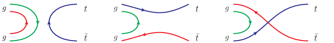
Figure 15: Color-flow diagrams in the $gg\to t\bar{t}$ amplitudes. Left diagram representing the color-factor $\delta^{ab}\delta_{ij}$ is for the color-singlet case, middle and right diagrams representing the color-factor $(T^{a}T^{b})_{ij}$ and $(T^{b}T^{a})_{ij}$, respectively, are for the color-octet case.

Appendix D Dilepton distributions in dilepton decay mode

In the main body of this paper we assume that the $W$-bosons from top-quark decays are on-shell. In this appendix, we take into account decays of the $W$-bosons at the matrix-element level. The advantage is to correctly take into account the off-shellness and polarization of the $W$-bosons. This is crucial to predict correctly the angular distributions as well as other kinematical distributions of the decay daughters of $W$’s. As an example, we show some distributions in the dilepton decay mode $pp\to bW^{+}\bar{b}W^{-}\to b\ell^{+}\nu_{\ell}\bar{b}\ell^{-}\bar{\nu}_{\ell}$, where $\ell=e$, $\mu$.

We calculate the amplitudes from the set of Feynman diagrams obtained by just adding the $W\to\ell\nu_{\ell}$ vertex to the Feynman diagrams for the $bW^{+}\bar{b}W^{-}$ final state. We generate the dilepton events at the LHC $\sqrt{s}=14$ TeV with standard kinematical cuts for the lepton momenta, $|\eta_{\ell}|\leq 2.5$ and $p_{T,\ell}\geq 10$ GeV. To avoid a singularity due to the vanishing running top-quark width, see Eq. (43) in Appendix B, we restrict the phase-space integral region to $m_{bW}>m_{b}+m_{W}$. Note that the matrix-elements for $m_{bW}<m_{b}+m_{W}$ are very suppressed. We set the $W$-boson decay-width to $\Gamma_{W}=2.05$ GeV.

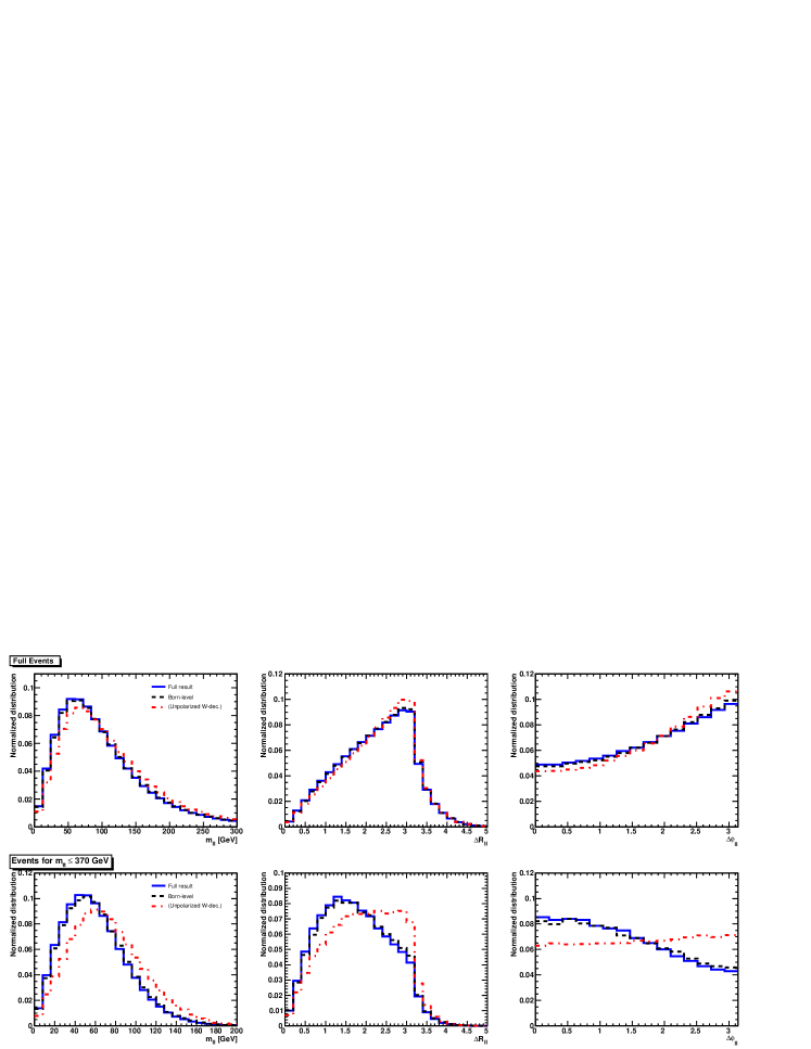
Figure 16: Distributions in an invariant-mass (left), a distance in $\eta$-$\phi$ plane (middle), and a difference in the azimuthal angle (right) of the two leptons for the dilepton events at the LHC $\sqrt{s}=14$ TeV. Top three graphs are for the full events, and bottom three graphs are for the events with $m_{t\bar{t}}\leq 370$ GeV. Blue solid line is the full result, blue dashed line is the Born-level result, and red dot-dashed line is obtained by the full calculation but assuming unpolarized $W$-bosons.

In Figs. 16, we plot three different distributions of kinematical variables constructed from the four-momenta of dileptons: (a1, a2) the invariant-mass of the two leptons, (b1, b2) the distance in the $\eta$-$\phi$ plane, $\Delta{R}_{\ell\ell}=\sqrt{\Delta\eta_{\ell\ell}^{2}+\Delta\phi_{\ell\ell}^{2}}$, and (c1, c2) the difference of the azimuthal angles, $\Delta\phi_{\ell\ell}$. The first three graphs (a1, b1, c1) correspond to the events from all the $m_{t\bar{t}}$ region, while the last three (a2, b2, c2) to the events with $m_{t\bar{t}}\leq 370$ GeV. The solid lines represent our full prediction, and the dashed lines represent the Born-level predictions. To see the effects of the non-zero $W$-boson polarization, we also plot the distributions computed from the $bW^{+}\bar{b}W^{-}$ events followed by the leptonic decays of on-shell unpolarized $W$-bosons.

We find that, due to the bound-state corrections, all three distributions are shifted to the lower side, although the variations are fairly small even for the events with $m_{t\bar{t}}\leq 370$ GeV. By contrast, the effects of the non-zero $W$-boson polarization is pronounced, especially for the events with $m_{t\bar{t}}\leq 370$ GeV. The most evident difference can be seen in the $\Delta\phi_{\ell\ell}$ distribution, where the full calculation predicts that the number of events at $\Delta\phi_{\ell\ell}=0$ is more than twice than the number of events at $\Delta\phi_{\ell\ell}=\pi$, while almost flat distribution by assuming the unpolarized $W$-bosons.

This finding is consistent with the similar study in Ref. [17] where the importance of the top-quark spin correlation in the $\Delta\phi_{\ell\ell}$ distribution is examined for the events with $m_{t\bar{t}}\leq 400$ GeV. They compare the $\Delta\phi_{\ell\ell}$ distribution fully taking into account the top-quark spin correlation with that assuming the spherical top-quark decay into $bW$’s followed by the correlated $W$-boson decay. Our calculation assuming unpolarized $W$-boson decays includes the correct angular distributions in $t\to bW$ decays, but forcing spherical distributions in $W\to\ell\nu_{\ell}$ decays. Thus, to predict the dilepton observables, all the spin correlations in decays of top-quarks and also $W$-bosons are required. We confirm their finding that the difference in $\Delta{R}_{\ell\ell}$ distribution comes from mainly the difference in $\Delta\phi_{\ell\ell}$ distribution.

References

- [1] S. Moch and P. Uwer, “Theoretical status and prospects for top-quark pair production at hadron colliders,” Phys. Rev. D 78 (2008) 034003 [arXiv:0804.1476 [hep-ph]].
- [2] M. Cacciari, S. Frixione, M. L. Mangano, P. Nason and G. Ridolfi, “Updated predictions for the total production cross sections of top and of heavier quark pairs at the Tevatron and at the LHC,” JHEP 0809 (2008) 127 [arXiv:0804.2800 [hep-ph]].
- [3] N. Kidonakis and R. Vogt, “The Theoretical top quark cross section at the Tevatron and the LHC,” Phys. Rev. D 78 (2008) 074005 [arXiv:0805.3844 [hep-ph]].
- [4] W. Bernreuther, “Top quark physics at the LHC,” J. Phys. G 35 (2008) 083001 [arXiv:0805.1333 [hep-ph]].
- [5] [Tevatron Electroweak Working Group and CDF Collaboration and D0 Collab], “Combination of CDF and D0 Results on the Mass of the Top Quark,” arXiv:0903.2503 [hep-ex].
- [6] C. Amsler et al. [Particle Data Group], “Review of particle physics,” Phys. Lett. B 667 (2008) 1.
- [7] P. Nason, S. Dawson and R. K. Ellis, “The Total Cross-Section For The Production Of Heavy Quarks In Hadronic Collisions,” Nucl. Phys. B 303 (1988) 607.
- [8] W. Beenakker, H. Kuijf, W. L. van Neerven and J. Smith, “QCD Corrections to Heavy Quark Production in p anti-p Collisions,” Phys. Rev. D 40 (1989) 54.
- [9] S. Catani, M. L. Mangano, P. Nason and L. Trentadue, “The Top Cross Section in Hadronic Collisions,” Phys. Lett. B 378 (1996) 329 [arXiv:hep-ph/9602208].
- [10] N. Kidonakis and G. Sterman, “Resummation for QCD hard scattering,” Nucl. Phys. B 505 (1997) 321 [arXiv:hep-ph/9705234].
- [11] R. Bonciani, S. Catani, M. L. Mangano and P. Nason, “NLL resummation of the heavy-quark hadroproduction cross-section,” Nucl. Phys. B 529 (1998) 424 [arXiv:hep-ph/9801375].
- [12] M. L. Mangano, P. Nason and G. Ridolfi, “Heavy quark correlations in hadron collisions at next-to-leading order,” Nucl. Phys. B 373 (1992) 295.
- [13] S. Frixione, M. L. Mangano, P. Nason and G. Ridolfi, “Top quark distributions in hadronic collisions,” Phys. Lett. B 351 (1995) 555 [arXiv:hep-ph/9503213].
- [14] W. Bernreuther, A. Brandenburg, Z. G. Si and P. Uwer, “Top quark pair production and decay at hadron colliders,” Nucl. Phys. B 690 (2004) 81 [arXiv:hep-ph/0403035].
- [15] R. Frederix and F. Maltoni, “Top pair invariant mass distribution: a window on new physics,” JHEP 0901 (2009) 047 [arXiv:0712.2355 [hep-ph]].
- [16] K. Melnikov and M. Schulze, “NLO QCD corrections to top quark pair production and decay at hadron colliders,” JHEP 0908 (2009) 049 [arXiv:0907.3090 [hep-ph]].
- [17] G. Mahlon and S. J. Parke, “Spin Correlation Effects in Top Quark Pair Production at the LHC,” Phys. Rev. D 81 (2010) 074024 [arXiv:1001.3422 [hep-ph]].
- [18] W. Bernreuther and Z. G. Si, “Distributions and correlations for top quark pair production and decay at the Tevatron and LHC,” Nucl. Phys. B 837, 90 (2010) [arXiv:1003.3926 [hep-ph]].
- [19] S. Biswas, K. Melnikov and M. Schulze, “Next-to-leading order QCD effects and the top quark mass measurements at the LHC,” arXiv:1006.0910 [hep-ph].
- [20] K. Hagiwara, Y. Sumino and H. Yokoya, “Bound-state Effects on Top Quark Production at Hadron Colliders,” Phys. Lett. B 666 (2008) 71 [arXiv:0804.1014 [hep-ph]].
- [21] Y. Kiyo, J. H. Kuhn, S. Moch, M. Steinhauser and P. Uwer, “Top-quark pair production near threshold at LHC,” Eur. Phys. J. C 60 (2009) 375 [arXiv:0812.0919 [hep-ph]].
- [22] K. Fujii, T. Matsui and Y. Sumino, “Physics at t anti-t threshold in e+ e- collisions,” Phys. Rev. D 50 (1994) 4341.
- [23] M. Martinez and R. Miquel, “Multi-parameter fits to the t anti-t threshold observables at a future e+ e- linear collider,” Eur. Phys. J. C 27, 49 (2003) [arXiv:hep-ph/0207315].
- [24] K. Ikematsu, K. Fujii, Z. Hioki, Y. Sumino and T. Takahashi, “How well can we reconstruct the system near its threshold at future linear colliders?,” Eur. Phys. J. C 29 (2003) 1 [arXiv:hep-ph/0302214].
- [25] Y. Sumino, K. Fujii, K. Hagiwara, H. Murayama and C. K. Ng, “Top quark pair production near threshold,” Phys. Rev. D 47 (1993) 56.
- [26] M. Jezabek, J. H. Kuhn and T. Teubner, “Momentum distributions in t anti-t production and decay near threshold,” Z. Phys. C 56 (1992) 653.
- [27] V. S. Fadin and V. A. Khoze, “Threshold Behavior of Heavy Top Production in e+ e- Collisions,” JETP Lett. 46 (1987) 525 [Pisma Zh. Eksp. Teor. Fiz. 46 (1987) 417].
- [28] V. S. Fadin and V. A. Khoze, “Production of a pair of heavy quarks in e+ e- annihilation in the threshold region,” Sov. J. Nucl. Phys. 48 (1988) 309 [Yad. Fiz. 48 (1988) 487].
- [29] A. H. Hoang et al., “Top-antitop pair production close to threshold: Synopsis of recent NNLO results,” Eur. Phys. J. direct C 2 (2000) 1 [arXiv:hep-ph/0001286], and references therein.
- [30] N. Kauer, “Top pair production beyond double pole approximation: , six fermions and zero, one or two additional partons,” Phys. Rev. D 67 (2003) 054013 [arXiv:hep-ph/0212091].
- [31] M. Beneke, B. Jantzen and P. Ruiz-Femenia, “Electroweak non-resonant NLO corrections to e+ e- W+ W- b bbar in the t tbar resonance region,” arXiv:1004.2188 [hep-ph].
- [32] F. Maltoni and T. Stelzer, “MadEvent: Automatic event generation with MadGraph,” JHEP 0302 (2003) 027 [arXiv:hep-ph/0208156].
- [33] J. Alwall et al., “MadGraph/MadEvent v4: The New Web Generation,” JHEP 0709 (2007) 028 [arXiv:0706.2334 [hep-ph]].
- [34] S. Frixione and B. R. Webber, “Matching NLO QCD computations and parton shower simulations,” JHEP 0206 (2002) 029 [arXiv:hep-ph/0204244].
- [35] S. Frixione, P. Nason and B. R. Webber, “Matching NLO QCD and parton showers in heavy flavour production,” JHEP 0308 (2003) 007 [arXiv:hep-ph/0305252].
- [36] S. Frixione, P. Nason and G. Ridolfi, “A Positive-Weight Next-to-Leading-Order Monte Carlo for Heavy Flavour Hadroproduction,” JHEP 0709 (2007) 126 [arXiv:0707.3088 [hep-ph]].
- [37] V B Berestetskii, L. P. Pitaevskii, E.M. Lifshitz, “Quantum Electrodynamics,” Second Edition, Butterworth-Heinemann.
- [38] B. A. Kniehl, A. A. Penin, Y. Schroder, V. A. Smirnov and M. Steinhauser, “Two-loop static QCD potential for general colour state,” Phys. Lett. B 607, 96 (2005) [arXiv:hep-ph/0412083], and references therein.
- [39] A. Denner, S. Dittmaier, M. Roth and D. Wackeroth, “Predictions for all processes e+ e- 4fermions + gamma,” Nucl. Phys. B 560, 33 (1999) [arXiv:hep-ph/9904472].
- [40] A. Denner, S. Dittmaier, M. Roth and L. H. Wieders, “Electroweak corrections to charged-current e+ e- 4 fermion processes: Technical details and further results,” Nucl. Phys. B 724, 247 (2005) [arXiv:hep-ph/0505042].
- [41] A. H. Hoang and C. J. Reisser, “Electroweak absorptive parts in NRQCD matching conditions,” Phys. Rev. D 71, 074022 (2005) [arXiv:hep-ph/0412258].
- [42] A. H. Hoang, C. J. Reisser and P. Ruiz-Femenia, Phys. Rev. D 82, 014005 (2010) [arXiv:1002.3223 [hep-ph]].
- [43] M. E. Luke, A. V. Manohar and I. Z. Rothstein, “Renormalization group scaling in nonrelativistic QCD,” Phys. Rev. D 61, 074025 (2000) [arXiv:hep-ph/9910209].
- [44] A. H. Hoang and I. W. Stewart, “Ultrasoft renormalization in non-relativistic QCD,” Phys. Rev. D 67, 114020 (2003) [arXiv:hep-ph/0209340].
- [45] M. Beneke, A. P. Chapovsky, A. Signer and G. Zanderighi, “Effective theory approach to unstable particle production,” Phys. Rev. Lett. 93, 011602 (2004) [arXiv:hep-ph/0312331].
- [46] M. Beneke, A. P. Chapovsky, A. Signer and G. Zanderighi, “Effective theory calculation of resonant high-energy scattering,” Nucl. Phys. B 686, 205 (2004) [arXiv:hep-ph/0401002].
- [47] M. Peter and Y. Sumino, “Final-state interactions in e+ e- t anti-t b l+ nu anti-b W- near top quark threshold,” Phys. Rev. D 57 (1998) 6912 [arXiv:hep-ph/9708223].
- [48] M. Jezabek and T. Teubner, “Momentum distributions in t anti-t production and decay near threshold. 2. Momentum dependent width,” Z. Phys. C 59 (1993) 669.
- [49] W. Modritsch and W. Kummer, “Relativistic And Gauge Independent Off-Shell Corrections To The Toponium Decay Width,” Nucl. Phys. B 430 (1994) 3.
- [50] W. Kummer and W. Modritsch, “Relativistic bound state equation for unstable fermions and the toponium width,” Phys. Lett. B 349 (1995) 525 [arXiv:hep-ph/9501406].
- [51] T. Sjostrand, S. Mrenna and P. Skands, “PYTHIA 6.4 Physics and Manual,” JHEP 0605 (2006) 026 [arXiv:hep-ph/0603175].
- [52] G. Corcella et al., “HERWIG 6.5: an event generator for Hadron Emission Reactions With Interfering Gluons (including supersymmetric processes),” JHEP 0101 (2001) 010 [arXiv:hep-ph/0011363].
- [53] M. Beneke, P. Falgari and C. Schwinn, “Soft radiation in heavy-particle pair production: all-order colour structure and two-loop anomalous dimension,” Nucl. Phys. B 828 (2010) 69 [arXiv:0907.1443 [hep-ph]].
- [54] M. Beneke, M. Czakon, P. Falgari, A. Mitov and C. Schwinn, “Threshold expansion of the gg(qq) QQ+X cross section at O(),” Phys. Lett. B 690 (2010) 483 [arXiv:0911.5166 [hep-ph]].
- [55] V. Ahrens, A. Ferroglia, M. Neubert, B. D. Pecjak and L. L. Yang, “Renormalization-Group Improved Predictions for Top-Quark Pair Production at Hadron Colliders,” arXiv:1003.5827 [hep-ph].
- [56] J. Pumplin, D. R. Stump, J. Huston, H. L. Lai, P. M. Nadolsky and W. K. Tung, “New generation of parton distributions with uncertainties from global QCD analysis,” JHEP 0207 (2002) 012 [arXiv:hep-ph/0201195].
- [57] A. D. Martin, W. J. Stirling, R. S. Thorne and G. Watt, “Parton distributions for the LHC,” Eur. Phys. J. C 63 (2009) 189 [arXiv:0901.0002 [hep-ph]].
- [58] T. Stelzer and W. F. Long, “Automatic generation of tree level helicity amplitudes,” Comput. Phys. Commun. 81 (1994) 357 [arXiv:hep-ph/9401258].
- [59] H. Murayama, I. Watanabe and K. Hagiwara, “HELAS: HELicity amplitude subroutines for Feynman diagram evaluations,” KEK-91-11.
- [60] S. Kawabata, “A New Monte Carlo Event Generator For High-Energy Physics,” Comput. Phys. Commun. 41 (1986) 127.
- [61] S. Frixione, E. Laenen, P. Motylinski and B. R. Webber, “Angular correlations of lepton pairs from vector boson and top quark decays in Monte Carlo simulations,” JHEP 0704 (2007) 081 [arXiv:hep-ph/0702198].
- [62] Y. Sumino, “Static QCD potential at r Lambda(QCD)**(-1): Perturbative expansion and operator-product expansion,” Phys. Rev. D 76, 114009 (2007) [arXiv:hep-ph/0505034].
- [63] D. Lurié, A. MacFarlane and Y. Takahashi, “Normalization of Bethe-Salpeter wave functions,” Phys. Rev. 140B (1965) 1091.
- [64] P. Artoisenet, F. Maltoni and T. Stelzer, “Automatic generation of quarkonium amplitudes in NRQCD,” JHEP 0802 (2008) 102 [arXiv:0712.2770 [hep-ph]].