Local quenches in frustrated quantum spin chains: global vs. subsystem equilibration

Abstract

We study the equilibration behavior following local quenches, using frustrated quantum spin chains as an example of interacting closed quantum systems. Specifically, we examine the statistics of the time series of the Loschmidt echo, the trace distance of the time-evolved local density matrix to its average state, and the local magnetization. Depending on the quench parameters, the equilibration statistics of these quantities show features of good or poor equilibration, indicated by Gaussian, exponential or bistable distribution functions. These universal functions provide valuable tools to characterize the various time-evolution responses and give insight into the plethora of equilibration phenomena in complex quantum systems.

I Introduction

The equilibration properties of closed quantum systems have been a topic of growing interest. As opposed to equilibration in open quantum systems coupled to an infinite bath, a closed finite quantum system does not admit asymptotic fixed points, unless the initial state is an eigenstate of the evolution Hamiltonian. Except for this trivial case, the evolution state $\rho\left(t\right)$ oscillates without converging to any limiting point. On the other hand, equilibration in closed quantum systems may be defined by resorting to probabilistic notions von Neumann (1929); Tasaki (1998); Popescu et al. (2006); Linden et al. (2009); Reimann (2008); Goldstein et al. (2010). Specifically, one says that an observable equilibrates if it remains close to its average for most of the times along the evolution trajectory. Alternatively, equilibration takes place if the fluctuations around the average are small. For typical initial states, the authors of Popescu et al. (2006); Linden et al. (2009) proved a number of bounds on the fluctuations that imply equilibration, provided the subsystem is small compared to the environment. Here “typical” means “taken uniformly at random from the space of pure states”. The insightful results in Popescu et al. (2006); Linden et al. (2009) leave nonetheless open the question of equilibration for a number of interesting cases. Namely when sizes are such that the environment cannot be considered overwhelmingly larger than the subsystems and/or when the initial state cannot be considered typical. Both such features are present in the experimentally relevant situation of small quenches on a finite system Roux (2010); Biroli et al. (2009). This is the situation studied in this article. More precisely, we suddenly change the evolution Hamiltonian only on a subsystem $S$ and then monitor equilibration features of the subsystem as well as of the total system by studying the full statistics of global (i.e. with support on the whole system) as well as of local observables. For the local subsystem we choose the subsystem magnetization as a physically natural observable. To obtain information on all possible observables defined on $S$ we monitor the trace distance of the subsystem density matrix from its equilibrium value. As a global observable we take the Loschmidt echo (LE). The Loschmidt echo has the additional appealing features that its time averages provides a bound on the fluctuations on any sufficiently small subsystem. However, in the situations under study most of the bounds are too loose and equilibration must be checked by an explicit computation.

To be more specific, the idea is the following. We prepare the system at $t=0$ in the ground state of the Hamiltonian $H_{0}$. At $t>0$ we suddenly modify the Hamiltonian in the region $S$. The system then evolves without further disturbance with Hamiltonian $H=H_{0}+V_{S}$, where the term $V_{S}$ only acts on subsystem $S$. The equilibration properties are then evaluated by monitoring local quantities of $S$ as well as global quantities of the entire system. Throughout this paper we will use the terms “local” resp. “global” for quantities which refer to subsystem $S$ resp. the entire system. The idea is to study the interplay between equilibration of these “local” and “global” quantities.

After a sufficiently long evolution time, the trajectory $\rho\left(t\right)$ defines an emerging equilibrium average ensemble given by $\overline{\rho}:=\overline{\rho\left(t\right)}:=\lim_{T\to\infty}T^{-1}\int_{0}^{T}\rho\left(t\right)$, where the observation time $T$ has been sent to infinity. The average density matrix $\overline{\rho}$, in the eigenbasis of the evolution Hamiltonian $H$, has the form of a dephased state: $\overline{\rho}=\sum_{n}p_{n}|n\rangle\langle n|,$ where $p_{n}=\left|\langle n|\psi_{0}\rangle\right|^{2}$ ($|\psi_{0}\rangle$ initial state), and for simplicity we assume here that the eigenenergies $E_{n}$ are non-degenerate Reimann (2008); Linden et al. (2009). In the same fashion, if we monitor an observable $O$ over a long time, its average value will be given by $\overline{O}:=\overline{\langle O\left(t\right)\rangle}:=\overline{\mathrm{tr}\left[\rho\left(t\right)O\right]}$. In finite systems we can safely bring the time average inside the trace and obtain $\overline{O}=\mathrm{tr}\left[\overline{\rho}O\right]$. The equilibration properties of an observable are encoded in its variance, or more precisely in its full statistics. The quantity $\langle O\left(t\right)\rangle$ is seen as a stochastic variable with the uniform measure $dt/T$ over the observation time interval $\left[0,T\right]$ ($T$ will be sent to infinity). We can say that the observable $O$ has good equilibration features if its probability distribution $P_{O}$ shows concentration around its mean value. Explicitly, the probability distribution $P_{O}$ is given by $P_{O}\left(x\right)=\overline{\delta\left(\langle O\left(t\right)\rangle-x\right)}$. To fix ideas further, we can say that good equilibration corresponds to a small variance $\overline{\Delta O^{2}}$, or more precisely to a large signal to noise ratio $\overline{O}/\sqrt{\overline{\Delta O^{2}}}$. Clearly $P_{O}$ depends on the observable $O$ but also on the initial state $|\psi_{0}\rangle$ and on the evolution Hamiltonian $H$.

II Preliminaries

The model we study here is the frustrated antiferromagnetic Heisenberg spin-1/2 chain, with a magnetic field acting only on a subsystem $S$ containing $N_{S}$ adjacent sites. Its Hamiltonian is given by

$$H=\sum_{j=1}^{N}\left(J_{1}\boldsymbol{S}_{j}\cdot\boldsymbol{S}_{j+1}+J_{2}\boldsymbol{S}_{j}\cdot\boldsymbol{S}_{j+2}\right)-h_{S}\sum_{j=1}^{N_{S}}S_{j}^{z},$$ (1)

where $J_{1}$ and $J_{2}$ denote the nearest-neighbor and next-nearest-neighbor couplings respectively, $J_{1}$ is set to 1 hereafter, $\boldsymbol{S}_{j}$ are spin-1/2 operators, and periodic boundary conditions are applied throughout, i.e. $\boldsymbol{S}_{j+N}=\boldsymbol{S}_{j}$. The initial, i.e. pre-quench, Hamiltonian $H_{0}$ is given by Eq. (1) with $h_{S}=h_{S}^{\left(i\right)}$. The local field $h_{S}$ is then suddenly changed, such that the evolution Hamiltonian $H$ is given by Eq. (1) with $h_{S}=h_{S}^{\left(f\right)}$. The couplings $J_{1},\,J_{2}$ are held fixed during the quench process.

If we consider the hard-core boson mapping of the spin variables given by $S_{j}^{z}=b_{j}^{\dagger}b_{j}-1/2$, the local field $h_{S}$ is equivalent to a local chemical potential which confines the particles in region $S$. The Hamiltonian Eq. (1) commutes with the total magnetization $S_{\mathrm{tot}}^{z}$. Since in the numerical studies discussed below the initial field $h_{S}$ is not chosen excessively large, we verified that the ground state of $H_{0}$ (and so the evolved state too) always belongs to the sector with zero total magnetization $S_{\mathrm{tot}}^{z}=0$. This means that the system has $N/2$ hard core bosons which initially prefer to occupy the region $S$; still the hard-core constraint ($(b_{j}^{\dagger})^{2}=0$) does not permit to have more than one particle at the same site .

The local field also breaks translational invariance. This enlarges the dimension $d_{0}$ of the ground state manifold, i.e. the vector space which contains the starting state, $|\psi_{0}\rangle$ and the evolved state $|\psi\left(t\right)\rangle=\exp\left(-itH\right)|\psi_{0}\rangle$. This feature is important. In fact, $d_{0}$ plays the role of an effective Hilbert space dimension. In systems with many symmetries, $d_{0}$ can be significantly reduced with respect to the total Hilbert space dimension. As a consequence, a system with large $d_{0}$ has comparatively smaller finite size effects compared to a system with the same number of sites but more symmetries and smaller $d_{0}$.

To obtain information about the system’s equilibration properties we consider various time dependent observables $f\left(t\right)$ and compute their statistics using the uniform measure $dt/T$ over the interval $\left[0,T\right]$, in other words we compute the probability distribution $P_{f}$ of the random variable $f\left(t\right)$ via $P_{f}\left(x\right):=\overline{\delta\left(f\left(t\right)-x\right)}$. We are mainly interested in the concentration properties of $P_{f}$, that is its “peakedness”.

To monitor what happens to subsystem $S$ we first consider its magnetization $m_{S}\left(t\right):=\langle S_{S}^{z}\left(t\right)\rangle/N_{S}=\langle\psi\left(t\right)|S_{S}^{z}|\psi\left(t\right)\rangle/N_{S}$. As for any other observable $O$, it can be expressed in the basis of the eigenvectors of the evolution Hamiltonian in the following way:

$$\langle O\left(t\right)\rangle=\overline{O}+\sum_{n>m}2\langle n|O|m\rangle c_{m}c_{n}\cos\left[t\left(E_{m}-E_{n}\right)\right].$$ (2)

Here $c_{n}=\langle n|\psi_{0}\rangle$, and we assumed that both the observable $O$ and the initial state $|\psi_{0}\rangle$ can be chosen real in the basis of $H$.

The local magnetization $S_{S}^{z}$, although being quite natural, is just one of the $2^{N_{S}}$ linearly independent observables which we can define on $S$. To obtain information on all possible observables on $S$ one has to consider the density matrix of the subsystem $S$: $\rho_{S}\left(t\right)=\mathrm{tr}_{\overline{S}}|\psi\left(t\right)\rangle\langle\psi\left(t\right)|$. A convenient quantity which encodes the equilibration properties of all observables in $S$ is then given by the trace distance between $\rho_{S}\left(t\right)$ and its equilibrium value $\overline{\rho_{S}}$, i.e.

$$D_{S}\left(t\right):=\left\|\rho_{S}\left(t\right)-\overline{\rho_{S}}\right\|_{1},$$ (3)

where the norm-1 of a matrix $O$ is given by $\left\|O\right\|_{1}:=\frac{1}{2}\mathrm{tr}\sqrt{O^{\dagger}O}$. The trace distance $D_{S}$ in Eq. (3) was first considered in Linden et al. (2009). If the time average of $D_{S}\left(t\right)$ is small, the evolved state of the subsystem $\rho_{S}\left(t\right)$ stays close to its average $\overline{\rho_{S}}$ for most of the time. This can be made quantitative by noting that $D_{S}$ is a positive quantity and using Markov’s inequality:

$$\mathrm{Prob}\left[D_{S}\left(t\right)\geq\epsilon\right]\leq\frac{\overline{D_{S}}}{\epsilon},$$

valid for any positive $\epsilon$. This implies that, for any observable $O$ defined on $S$, the time evolved quantity $\langle O\left(t\right)\rangle$ is close to its mean $\overline{O}$ for most of the time. That is if $\overline{D_{S}}$ is small, then one finds good equilibration for all observables in $S$. This can be shown by noting that, if the observable $O$ has its spectrum in $\left[o_{\mathrm{min}},o_{\mathrm{max}}\right]$ then Linden et al. (2009):

$$\left|\mathrm{tr}[\rho_{S}(t)O]-\mathrm{tr}[\overline{\rho_{S}}O]\right|\leq\left(o_{\mathrm{max}}-o_{\mathrm{min}}\right)D_{S}(t).$$ (4)

The authors of Linden et al. (2009) also proved the following interesting inequalities

$$\overline{D_{S}}\leq\frac{1}{2}\sqrt{\frac{d_{S}}{d^{\mathrm{eff}}\left(\overline{\rho}_{\overline{S}}\right)}}\leq\frac{1}{2}\sqrt{\frac{d_{S}^{2}}{d^{\mathrm{eff}}\left(\overline{\rho}\right)}}.$$ (5)

Here $d_{S}$ is the dimension of subsystem $S$, equal to $2^{N_{S}}$ in our case, the effective dimension of a density matrix $d^{\mathrm{eff}}\left(\sigma\right)$ is defined as the inverse purity, i.e. $d^{\mathrm{eff}}\left(\sigma\right)=1/\mathrm{tr}\left(\sigma^{2}\right)$. Finally, $\overline{\rho}_{\overline{S}}$ is the equilibrium state restricted to the complementary of $S$, i.e. its environment $\overline{S}$. Especially the second inequality of Eq. (5) is very useful. It gives a bound on $\overline{D_{S}}$ by resorting to a global quantity $d^{\mathrm{eff}}\left(\overline{\rho}\right)$. As was shown in Linden et al. (2009); Campos Venuti and Zanardi (2010a, b), for large quenches $1/d^{\mathrm{eff}}\left(\overline{\rho}\right)$ is typically exponentially small in the system size: $1/d^{\mathrm{eff}}\left(\overline{\rho}\right)\approx\exp\left(-\mathrm{const.}\times N\right)$. There is, however, an interplay between system size and quench amplitude. For moderate quenches, and/or when the system size is not too large, the constant appearing in the exponential can be very small. This can be seen using perturbation theory for small quenches which predicts Campos Venuti and Zanardi (2010a, b); Campos Venuti and Zanardi (2007) $1/d^{\mathrm{eff}}\left(\overline{\rho}\right)\approx\exp\left(-\mathrm{const.}\times\delta h_{S}^{2}\times N_{S}\right)$. Thus, when $N_{S}$ is not large compared to $(\delta h_{S})^{-2}$, the second bound in Eq. (5) is not effective, since $\overline{D_{S}}\leq 1$ by definition. Does this mean that equilibration in this case will not take place in subsystem $S$? This is precisely the question we are going to address here. Note that in our simulations with $N_{S}=4$ the second bound in Eq. (5) is not effective as long as $1/d^{\mathrm{eff}}\left(\overline{\rho}\right)\geq 0.015$, whereas in most of our simulations we have $1/d^{\mathrm{eff}}\left(\overline{\rho}\right)>0.9$ (see below).

As a prototype quantity to monitor global equilibration of the entire system, we study the Loschmidt echo (LE) Jarzynski (1997); Prosen (1998); Kurchan ; Jalabert and Pastawski (2001); Quan et al. (2006); Rossini et al. (2007a, b); Zanardi et al. (2007); Roux (2009)

$$\mathcal{L}\left(t\right)=\left|\langle\psi_{0}|\exp\left(-iHt\right)|\psi_{0}\rangle\right|^{2}.$$

Here $H$ is the evolution Hamiltonian, and $|\psi_{0}\rangle$ is the initial state. $\mathcal{L}\left(t\right)$ measures the probability that the state $|\psi\left(t\right)\rangle$ evolves back to the pre-quench initial state $|\psi_{0}\rangle$. In this sense, the LE is the expectation value of a particular operator, i.e. the projector onto the initial state $|\psi_{0}\rangle\langle\psi_{0}|$. This operator has clearly support on the entire system, and therefore the LE is the time dependent expectation value of a “global” quantity. The LE has many interesting interpretations (see e.g. Silva (2008); Campos Venuti and Zanardi (2010a) and reference therein). Most important for us, the time averaged LE is precisely the inverse of the effective quantum dimension defined above. In fact, writing the LE in the eigenbasis of $H$ one finds

$$\mathcal{L}\left(t\right)=\overline{\mathcal{L}}+2\sum_{n>m}p_{n}p_{m}\cos\left[t\left(E_{n}-E_{m}\right)\right],$$ (6)

where $\overline{\mathcal{L}}=\sum_{n}p_{n}^{2}=\mathrm{tr}\left(\overline{\rho}|\psi_{0}\rangle\langle\psi_{0}|\right)=\mathrm{tr}\left[(\overline{\rho})^{2}\right]=1/d^{\mathrm{eff}}\left(\overline{\rho}\right)$. Given its simple form in terms of the weights $p_{n}^{2}=\left|c_{n}\right|^{2}$, the probability distribution of the LE is closely related to the distribution of the $p_{n}$.

Once again, because of the bounds in Eqs. (5) and (4), a sufficiently small average of the LE implies equilibration in all (sufficiently small) subsystems. Moreover, using the bound $\overline{\mathcal{L}^{n}}\leq n!\overline{\mathcal{L}}^{n}$ proved in Campos Venuti and Zanardi (2010a) with $n=2$ we obtain that the variance satisfies $\overline{\Delta\mathcal{L}^{2}}\leq\overline{\mathcal{L}}^{2}$, and thus a small average implies small variance, with a signal to noise ratio greater or equal to 1. This scenario can be considered the standard road to equilibration. The converse need not be true, i.e. one can have a small variance for the LE but a large mean. The possibility of such alternative scenarios is what we are going to explore in this paper.

Details of the numerical computation: In the numerical computations we take advantage of conservation of total magnetization to reduce the Hilbert space dimension. To find the initial state $|\psi_{0}\rangle$, we first diagonalize $H_{0}$ in the lowest magnetization sectors, $S_{\mathrm{tot}}^{z}=0,1,2,3$, and keep the ground state. For the quench parameters used below we verified that $|\psi_{0}\rangle$ always belongs to the zero magnetization sector. We then diagonalize the evolution Hamiltonian $H$ using iterative Lanczos steps, calculating the first 500 hundred lowest energy eigenstates. To obtain a good approximation of the full sector we checked that the normalization condition was satisfied up to $10^{-4}$, i.e. $1-\sum_{n=1}^{500}p_{n}^{2}<10^{-4}$. The time series statistics of observables are obtained using 400,000 random samples in a time window $\left[0,T_{\mathrm{max}}\right]$ where $T_{\mathrm{max}}$ is chosen more than two orders of magnitude larger than the smallest energy gap in the system.

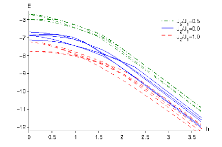
Figure 1: Lowest 5 energy levels of Hamiltonian Eq. (1) on a ring of $N=16$ sites for different coupling ratios $J_{2}/J_{1}$ as a function of the field $h_{S}$ applied on $N_{S}=4$ contiguous sites.

III Field-Energy-Dependence and Quenches in Different Regimes

The Hamiltonian (1) represents a fully interacting quantum system. In order to gain some initial insight into the physical properties of this system, we numerically calculate the five lowest energy levels of the model as a function of the applied local field $h_{S}$ on the four adjacent spins (representing the subsystem S) in a chain of 16 spins for different ratios of the nearest and next-nearest neighbor couplings (see Fig. 1).

Phase diagram at $h_{S}=0$: The phase diagram for the model at zero field and in the large $N$ limit is well known and has been described for example in Kwek et al. (2009). At zero field and $J_{2}=0$ we have a Heisenberg spin chain with only nearest-neighbor coupling, which is solvable using the Bethe Ansatz. For both positive $J_{1}$ and $J_{2}$ the system is frustrated. For small values of $J_{2}$ a gapless antiferromagnetic phase is present. At $J_{2}/J_{1}\approx 0.241$ a gap opens up, and the system remains gapped for all finite $J_{2}/J_{1}$, but the gap closes in the limit of $J_{2}/J_{1}\rightarrow\infty$, where the model is approximately described by two weakly coupled chains. At zero field and $J_{2}/J_{1}=1/2$ - the Majumdar-Ghosh point - the ground state of the system factorizes and can be determined analytically. Namely, the ground state manifold is two-fold degenerate spanned by $|\phi_{1}\rangle,\,|\phi_{2}\rangle$ where $|\phi_{1}\rangle$ consists of singlets between neighboring dimers, and $|\phi_{2}\rangle$ is $|\phi_{1}\rangle$ translated by one site.

The model in a finite local field: For small but finite local fields - roughly $h_{S}<0.3$ - we encounter a regime, in which the inter spin coupling dominates, and the local field acts as a perturbation. The dependence of the eigenenergies on the local field here is relatively flat. Degeneracies which occur for zero field are lifted.

For intermediate local fields - $0.5<h_{S}<2$ - the Heisenberg coupling and the local magnetic field compete. In this regime we observe numerous level crossings.

For large fields - $h_{S}>2.5$ - the energy levels are dominated by the applied local magnetic field, and thus simply decrease linearly with its amplitude. This is caused by the alignment of the affected spins along the field direction, i. e. $m_{S}\rightarrow 1/2$, thus maximizing the contribution of the Zeeman energy term, $E_{Zeeman}=-h_{S}\cdot N_{S}/2$. In this regime one can treat the Heisenberg interaction as a perturbation on the field Hamiltonian for the spins with an applied field. In this regime, the slope of all the energy levels in Fig. 1 approach what one would expect from a dominating Zeeman term $\frac{\partial E}{\partial h_{S}}\rightarrow N_{S}/2$.

Having these regimes of the model in mind, we consider the following quench scenarios: small quenches within each of the regimes and large quenches across different regimes.

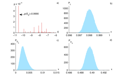
Figure 2: Equilibration statistics for $N=16$, $N_{S}=4$, $J_{2}/J_{1}=0$. The quench is from from $h_{S}^{(i)}/J_{1}=3.5$ to $h_{S}^{(f)}/J_{1}=3$. In panel a) the probabilities spectrum $p_{n}=p\left(E_{n}\right)$ is shown as a function of the energy. Panels b), c), d) show the full statistics of $P_{\mathcal{L}},\,P_{D_{S}},\,P_{m_{S}}$ respectively. Both the distribution of the LE and the magnetization are narrow Gaussian. Moreover $P_{D_{S}}$ indicates a small mean $\overline{D_{S}}$. All these facts indicate standard equilibration of Gaussian type. Qualitatively similar results are observed for different values of the ratio $J_{2}/J_{1}$.

The simplest case is a small quench within the regime of large dominating local fields, where the energy levels in good approximation simply vary linearly with the local field amplitude $h_{S}$. As an example of this case, we consider the quench from an initial field $h_{S}^{(i)}=3.5$ to an evolution field $h_{S}^{(f)}=3$ for the three different couplings $J_{2}/J_{1}=0,0.5,1$ (see Fig. 2). In all of these cases the Loschmidt Echo as well as the local magnetization show Gaussian distributions with very small variances, indicating a good, straightforward. This is exactly the behavior expected for small quenches in regular regimes Campos Venuti and Zanardi (2010a). The distribution of the quantity $D_{s}$ in these cases also resembles a Gaussian, only experiencing a slight asymmetry due to the non-linearity of the norm. So in regular regimes our example system shows good equilibration, both locally and globally.

Another set of relatively simple quenches are those from large fields to zero field. As the system in this case is strongly perturbed, one would expect numerous excitations across a wide range of energies. According to $\overline{\mathcal{L}}=1/d^{\mathrm{eff}}\left(\overline{\rho}\right)$ a large number of excitations causes a small Loschmidt Echo. More specifically such quenches lead to an exponential distribution of the Loschmidt Echo with an average very close to zero Campos Venuti and Zanardi (2010a). We numerically observe such a behavior when quenching from large to zero local magnetic fields for all three couplings. Figure 3 shows a representative example of a quench from $h_{S}^{(i)}=3$ to $h_{S}^{(f)}=0$ with only nearest-neighbor coupling. In this quench, one also obtains single peaked and relatively narrow distributions of the local magnetization and the quantity $D_{S}$. This indicates measure concentration and exactly the kind of strong local equilibration that is possible even for closed quantum systems which has been discussed in Linden et al. (2009). Results for different couplings are not shown here, but very similar.

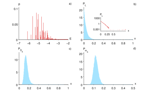
Figure 3: Equilibration statistics for $N=16$, $N_{S}=4$, $J_{2}/J_{1}=0$. The quench is from from $h_{S}^{(i)}/J_{1}=3$ to $h_{S}^{(f)}/J_{1}=0$. Panels as in figure 2. As can be seen from the log-linear plot in the inset of panel b), the distribution of the LE is exponential with a very small mean. Qualitatively similar results are observed for different values of the ratio $J_{2}/J_{1}$.

For small quenches in the regime of dominant Heisenberg couplings, we observe different types of equilibration and a strong dependence on the inter-spin coupling. This is discussed in the following section.

IV Numerical Results for non-trivial quenches

Here we investigate small quenches of the form $H_{0}(h_{S}^{(i)})\rightarrow H(h_{S}^{(f)})$ with $h_{S}^{(i)}=0.2$ and $h_{S}^{(f)}=0$ on systems of size $N=16$ and different coupling ratio. In particular we present three simulation for quenches on a subsystem $S$ of four spins ($N_{S}=4$) and coupling ratio $J_{2}/J_{1}=1,\,0,\,1/2$, and three analogous simulations for $N_{S}=3$. For all the simulations the initial ground state is located in the $S_{\mathrm{tot}}^{z}=0$ sector of vanishing total magnetization.

IV.1 Quenches on four adjacent spins

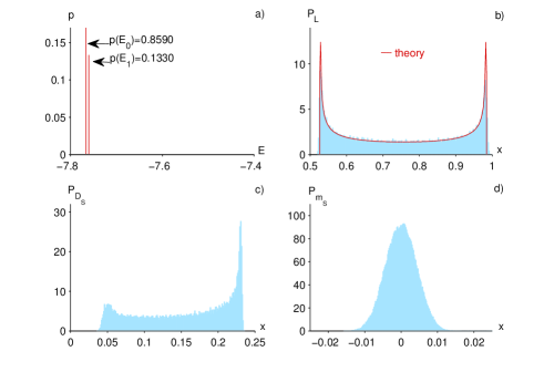
Figure 4: Quench 1. Equilibration statistics for $N=16$, $N_{S}=4$, $J_{2}/J_{1}=1$. The quench is from from $h_{S}^{(i)}/J_{1}=0.2$ to $h_{S}^{(f)}/J_{1}=0$. Panels as in figure 2.

Quench 1: The first example we consider is a quench on a system of equal nearest and next-nearest neighbor couplings ($J_{1}=J_{2}$). The system is quenched from $H_{0}(h_{S}^{(i)}=0.2)$ to $H(h_{S}^{(f)}=0)$. The resulting equilibration statistics are shown in Fig. 4. As one would expect for a small quench, the energy probability distribution $p(E_{n})$ in Fig. 4a) is dominated by the ground state ($p(E_{0})=0.86$). A more interesting feature is an additional sizable contribution of the first excited state. Note that the population of the first excited state is about two orders of magnitude larger than the population of all the others ($p(E_{1})\ll p(E_{i}),i>1$).

The existence of these two dominating modes leads to a double-peaked distribution function of the Loschmidt Echo $P_{\mathcal{L}}$, which is clearly observed in Fig. 4b). In this case, one can effectively neglect the weights $p_{n}$ with $n\geq 2$ in Eq. 6, and treat the model as an effective two-state system. Hence we obtain the following approximation for the Loschmidt echo

$$\mathcal{L}(t) \approx \underbrace{p_{0}^{2}+p_{1}^{2}}_{\approx\overline{\mathcal{L}}}+2p_{0}p_{1}\cos[(E_{1}-E_{0})t].$$ (7)

The corresponding probability distribution function can be calculated analytically:

$$P_{\mathcal{L}}(x)=\overline{\mathcal{L}}+\frac{1-\overline{\mathcal{L}}\left(x_{2}-x_{1}\right)}{\pi\sqrt{(x-x_{1})(x_{2}-x)}},$$ (8)

where $x_{1}=\overline{\mathcal{L}}-2p_{0}p_{1}$, $x_{2}=\overline{\mathcal{L}}+2p_{0}p_{1}$ denote the lower and upper edges of the distribution. Equation (8), with $p_{0}$ and $p_{1}$ obtained numerically, is shown as a red line in Fig. 4b) and shows excellent agreement with the full calculation. This result shows that, after the quench, the system oscillates between the two lowest states of $H$, $|0\rangle$ and $|1\rangle$, clearly indicating absence of equilibration. Such a lack of equilibration can also be observed in the variance, $\Delta\mathcal{L}=\left(x_{2}-x_{1}\right)/\sqrt{8}$ which is of the same order of the support of the distribution. Especially since the evolution Hamiltonian is translationally invariant, one would also expect to see this non-equilibrium behavior locally. Accordingly, the statistics of $D_{S}$ in Fig. 4c) shows lack of equilibration. Its distribution function also has a large spread and two maxima, one of which shows a similar divergence as the Loschmidt Echo. The asymmetry and the lack of a second peak are not numerical artifacts but arise due to the high non-linearity of the trace distance, namely its absolute value. A simplified example of this behavior is given in the Appendix.

It is interesting to note that the distribution of the local magnetization is Gaussian displaying good equilibration properties. The reason for this becomes clear when looking at Eq. (2). The largest (in modulus) contribution to that sum is given in principle by the term with $n=1$ and $m=0$, but this contribution vanishes as $\langle 1|O|0\rangle=0$. Hence the sum in Eq. (2) contains a large number of terms of the same order of magnitude. In this situation $\langle O\left(t\right)\rangle$ can be seen as a sum of many independent variable converging to a Gaussian thanks to a central limit theorem argument.

This situations makes clear that even when $\overline{D_{S}}$ is large one can still find observable (those with very small or zero weights in the low energy states) which show good equilibration properties .

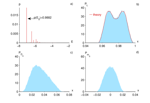
Figure 5: Quench 2. Equilibration statistics for $N=16$, $N_{S}=4$, $J_{2}/J_{1}=0$. The quench is from from $h_{S}^{(i)}/J_{1}=0.2$ to $h_{S}^{(f)}/J_{1}=0$. Panels as in figure 2.

Quench 2: The second quench we show is from a field of $h_{S}^{(i)}=0.2$ on four adjacent spins to zero field, but using only nearest-neighbor coupling, i.e. $J_{2}=0$. The energy probability distribution of this quench is shown in Fig. 5a). In this distribution the ground state is by far dominating ($p(E_{0})=0.99$), the probability of the next highest populated state is two orders of magnitudes smaller. Overall, there still is a concentration of excitations in the low energies ($E<-5.5$).

As indicated by the distribution of $p(E_{n})$, the Loschmidt Echo mean of this quench is much closer to one and its variance is about an order of magnitude smaller compared with the case $J_{2}=J_{1}$ (Fig. 5b)). Its distribution still shows two maxima, but they are less pronounced and smoother.

In general, a better approximation to the LE distribution function can be obtained by retaining the $N_{max}$ largest weights $W_{ij}=p_{i}p_{j}$ in equation (6). This procedure will be performed for all of the following quenches. For the quench discussed here, it is enough to keep $N_{max}=5$. The resulting approximate distribution is shown as a red line in Fig 5b).

Both the LE and $D_{S}$ indicate a much better equilibration compared to Quench 1. This is in contrast to the behavior of the local magnetization in Fig. 4d), which is again Gaussian, but shows a larger rather than a smaller variance.

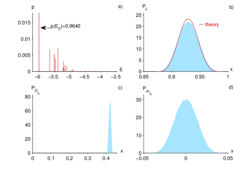
Figure 6: Quench 3. Equilibration statistics for $N=16$, $N_{S}=4$, $J_{2}/J_{1}=1/2$, Majumdar-Ghosh point. The quench is from from $h_{S}^{(i)}/J_{1}=0.2$ to $h_{S}^{(f)}/J_{1}=0$. Panels as in figure 2.

Quench 3: The last quench we want to discuss in detail is the special case of $J_{2}=1/2$. The evolution system in zero field is at the Majumdar-Ghosh point. The system has a two-fold degeneracy at its minimum energy, consisting of two states, each of them a product state of nearest-neighbor singlets. This degeneracy is lifted by the pre-quench applied local field, with $h_{S}^{(i)}=0.2$ acting on four adjacent spins. As a consequence the system cannot be treated as non-degenerate. To take the degeneracies into account the corresponding formulas have to be modified, e.g. $\overline{\rho}$ includes off-diagonal terms, where $E_{n}=E_{m}$ for $n\neq m$. Furthermore, because of degeneracies, the proof for inequality (5) given by Linden et al. (2009) does not hold in this case.

Inspecting $p(E_{n})$ in Fig. 6a), as in the case of $J_{2}=0$ the population of the ground energy level is by far dominating, $p(E_{0})=\mathrm{tr}\left[\Pi_{E_{0}}\rho_{0}\right]=0.96$ ($\Pi_{E_{0}}$ is the projector onto the bi-dimensional ground state manifold). We also observe many more excitations, none of which is considerably larger than the others. The distribution is concentrated at energies below $E=-5$, but even for $E>-5$ there are some weak excitations. Quite a few of the lowest energy eigenstates, are not populated at all, but protected by symmetry, e.g. $p(E_{1})=p(E_{2})=0$.

Since the $p(E_{n})$ are relatively widely distributed, and besides $p(E_{0})$ there is no other dominant contribution, we expect and numerically obtain a Gaussian distributed LE, as shown in Fig. 6. As in the previous quench we can approximate the LE truncating Eq. 6 to the first $N_{max}$ largest (in modulus) terms. As explained in Campos Venuti and Zanardi (2010b), in order to recover a Gaussian distribution we have take $N_{max}$ large, here $N_{max}=20$ is needed. The corresponding probability distribution is the line shown in Fig. 6b).

Compared to the quench at $J_{2}=0$ the LE mean is smaller and the distribution shows a higher variance. So far, this indicates relatively straightforward equilibration. Therefore the distribution of $D_{S}$ shown in Fig. 6c) is quite surprising. It shows a slightly asymmetric Gaussian with the lowest variance of all the quenches discussed, but with a relatively large mean $\overline{D_{S}}=0.419$.

A large $D_{S}$ does not mean bad equilibration for all local observables, but it indicates that there is at least one local observable, which equilibrates badly. As in the other quenches, the distribution function of the local magnetization is a Gaussian centered around zero. Here, in agreement with the LE, its variance is larger than in the case $J_{2}=1$.

IV.2 Quenches on three adjacent spins

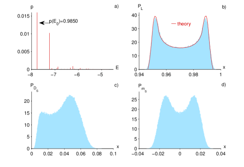
Figure 7: Quench 4. Equilibration statistics for $N=16$, $N_{S}=3$, $J_{2}/J_{1}=1$. The quench is from from $h_{S}^{(i)}/J_{1}=0.2$ to $h_{S}^{(f)}/J_{1}=0$. Panels as in figure 2.

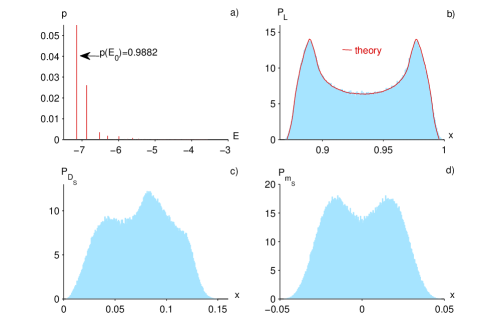
Figure 8: Quench 5. Equilibration statistics for $N=16$, $N_{S}=3$, $J_{2}/J_{1}=0$. The quench is from from $h_{S}^{(i)}/J_{1}=0.2$ to $h_{S}^{(f)}/J_{1}=0$. Panels as in figure 2.

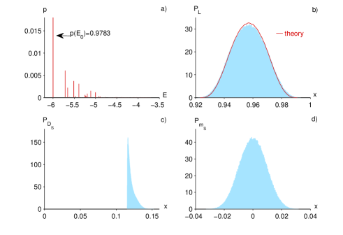
Figure 9: Quench 6. Equilibration statistics for $N=16$, $N_{S}=3$, $J_{2}/J_{1}=1/2$, Majumdar-Ghosh point. The quench is from from $h_{S}^{(i)}/J_{1}=0.2$ to $h_{S}^{(f)}/J_{1}=0$. Panels as in figure 2.

We also show the equilibration statics of the same three quenches just discussed, with the same quench amplitude but with a magnetic field acting on three instead that on four adjacent spins, i.e. $N=16$ and $N_{S}=3$ (Figs. 7-9). These quenches do not need to be discussed in the same detail, but indicate that some of the observed patterns are not restricted to $N_{S}=4$ and provide a few interesting other features. Note also that the corresponding variances of the considered observables $\mathcal{L}$, $D_{S}$ and $m_{S}$ in the case of $N_{S}=3$ are much smaller than for $N_{S}=4$.

Quench 4: In the case of $J_{2}/J_{1}=1$ (Fig. 7) one obtains a similar dominance of two lowest-energy modes as for the case $N_{S}=4$. Contributions of other states are only one order of magnitude smaller than the two dominating modes. The LE distribution accordingly is double peaked but smoother and with a wider spread compared to the 4-site local quench that is about an order of magnitude smaller. To obtain a good effective description using for the LE we use here $N_{max}=5$. The contribution of these few other states is even more visible in the distribution of $D_{S}$, which again shows two maxima, but is much less spiked. Differently from the case $N_{S}=4$, the local magnetization is double peaked following a distribution function similar to the one of the LE. Correspondingly the variance is roughly 4 times as large as for $N_{S}=4$, indicating worse equilibration. This can simply be explained by the fact that the two dominant modes, namely the ground state and the second excited state in this case have a finite cross term in the local magnetization.

Quench 5: The quench at $J_{2}/J_{1}=0$ shown in Fig. 8 displays similar features as in the case $J_{2}/J_{1}=1$, with all the distributions that tend to be broader.

Quench 6: The last quench shown in Fig. 9 is the case $J_{2}/J_{1}=1/2$, where the evolution Hamiltonian is at the Majumdar-Ghosh point. As in the case for $N_{S}=4$ one observes a relatively large number of non-vanishing modes and a Gaussian distribution of both the LE and the local magnetization. The approximation shown in Fig. 9b) is obtained using $N_{max}=10$. Although the distribution of $D_{S}$ is highly peaked with a small variance its average is relatively large, indicating that there can be local observables experiencing poor equilibration.

V Conclusions

In this paper we have numerically studied different local quantum quenches on frustrated spin chains. More precisely we considered both global and local equilibration indicators, the Loschmidt echo and the subsystem magnetization. To gain a better understanding of the equilibration properties of the subsystem we also studied the distance of the reduced density matrix from its time average: $D_{S}\left(t\right)=\left\|\rho_{S}\left(t\right)-\overline{\rho_{S}}\right\|$. Our numerical simulations show that a variety of possible scenarios take place depending on the interplay between quench amplitudes and coupling constants. In particular, for large and intermediate quenches the long time probability distribution of the Loschmidt echo resemble an exponential and a Gaussian respectively, as it was first observed in Campos Venuti and Zanardi (2010a). When the Loschmidt echo mean is very small the subsystem does equilibrate even when the bounds in Linden et al. (2009) are too loose to be applicable. On the contrary, when the Loschmidt echo mean is large and thus no general conclusion can be drawn a priori, we observe all possible situations. Namely we observe both cases where the subsystem equilibrates (quenches 2, 4) and where it does not (quenches 1, 3, 5, 6). Moreover even when the subsystem does not equilibrate as a whole, we still encounter instances where one observable (the magnetization) shows good equilibration properties (quenches 1, 3).

In conclusion, we would like to note that the identification and characterization of the time-scales associated with the different equilibration phenomena we observed lies outside the scope of the long-time statistics techniques adopted in this paper. Addressing this problem in its generality is perhaps the most exciting next challenge in the quest for understanding equilibration dynamics of unitarily evolving quantum systems.

P.Z. acknowledges support from NSF grants PHY-803304, DMR-0804914 and L.C.V. acknowledges support from European project COQUIT under FET-Open grant number 2333747.

Appendix

Let us assume that the system is divided into a subsystem $S$ and an environment $E$. The two corresponding bases are given by $\{\left|a\right>,\left|b\right>,\cdots\}$ and $\{\left|\alpha\right>,\left|\beta\right>,\cdots\}$. To model quench 1 and to simplify the calculation we further assume that only two eigenstates of the closed system $S\otimes E$ contribute to the full density matrix. (A reasonable simplification of the $p_{n}$ distribution in Fig. 4a).) To model the strongly coupled system and to obtain a non-unitary evolution of the subsystem, we have to introduce entanglement. This can be done by considering the two states

$$\left|1\right> \equiv \left(|a,\alpha\rangle+|b,\beta\rangle\right)/\sqrt{2},$$ (9)

$$\left|2\right> \equiv \left(|a,\alpha\rangle-|b,\beta\rangle\right)/\sqrt{2}.$$ (10)

Using the initial state $\left|\Psi_{0}\right>\equiv c_{1}\left|1\right>+c_{2}\left|2\right>$ we compute $D_{S}(t)$ and its distribution. Given the energy difference $\omega=E_{2}-E_{1}$ of the two eigenstates we obtain

$$\rho-\overline{\rho} = c_{1}c_{2}^{*}\left|1\right>\left<2\right|e^{-i\omega t}+h.c.$$ (11)

Tracing out the degrees of freedom of the bath this simplifies to

$$\rho_{S}-\overline{\rho_{S}} = \mathrm{Tr}_{B}\left(\rho-\overline{\rho}\right)$$ (12)

$$= c_{1}c_{2}^{*}\left(\left|a\right>\left<a\right|-\left|b\right>\left<b\right|\right)e^{i\omega t}+h.c..$$ (13)

Identifying $c_{1}c_{2}^{*}=\sqrt{p_{1}p_{2}}e^{i\varphi}$ and using a matrix representation we get

$$\rho_{S}-\overline{\rho_{S}} = \sqrt{p_{1}p_{2}}\cos\left(\omega t+\varphi\right)\left(\begin{array}[]{rr}1&0\\ 0&-1\end{array}\right)$$ (16)

We finally obtain

$$D_{S}(t) = \sqrt{p_{1}p_{2}}\left|\cos\left(\omega t+\varphi\right)\right|$$ (17)

Its distribution function can be calculated analytically, giving a simple description of a divergence similar to what we observe numerically,

$$P_{D_{S}}(x) = \lim\limits_{T\rightarrow\infty}\frac{1}{T}\int_{0}^{T}\delta\left(D_{S}\left(t\right)-x\right)dt$$ (18)

$$= \frac{\omega}{\pi}\int_{0}^{\frac{\pi}{\omega}}\delta\left(\sqrt{p_{1}p_{2}}\left|\cos\left(\omega t\right)\right|-x\right)dt$$ (19)

$$= \frac{2/\pi}{\sqrt{p_{1}p_{2}-x^{2}}}.$$ (20)

Note that in this case $D_{S}$ takes values in $D_{S}\in\left[0,\sqrt{p_{1}p_{2}}\right]$, so such a $P\left(d_{S}\right)$ has only one square root singularity at the upper edge. If we simply take the two largest amplitude contributions of Fig. 4a), we can estimate the peak in Fig. 4c) to be around $\sqrt{0.86\cdot 0.13}=0.33$. Given the great simplification this estimate is quite useful.

References

- von Neumann (1929) J. von Neumann, Zeitschrift für Physik 57, 30 (1929), see also the english translation by R. Tumulka at arXiv:1003.2133.
- Tasaki (1998) H. Tasaki, Phys. Rev. Lett. 80, 1373 (1998).
- Popescu et al. (2006) S. Popescu, A. J. Short, and A. Winter, Nature Physics 2, 754 (2006).
- Linden et al. (2009) N. Linden, S. Popescu, A. J. Short, and A. Winter, Phys. Rev. E 79, 061103 (2009).
- Reimann (2008) P. Reimann, Phys. Rev. Lett. 101, 190403 (2008).
- Goldstein et al. (2010) S. Goldstein, J. L. Lebowitz, R. Tumulka, , and N. Zanghí (2010), 1003.2129.
- Roux (2010) G. Roux, Phys. Rev. A 81, 053604 (2010).
- Biroli et al. (2009) G. Biroli, C. Kollath, and A. Läuchli (2009), arXiv:0907.3731.
- Campos Venuti and Zanardi (2010a) L. Campos Venuti and P. Zanardi, Phys. Rev. A 81, 022113 (2010a).
- Campos Venuti and Zanardi (2010b) L. Campos Venuti and P. Zanardi, Phys. Rev. A 81, 032113 (2010b).
- Campos Venuti and Zanardi (2007) L. Campos Venuti and P. Zanardi, Phys. Rev. Lett. 99, 095701 (2007).
- Jarzynski (1997) C. Jarzynski, Phys. Rev. Lett. 78, 2690 (1997).
- Prosen (1998) T. Prosen, Phys. Rev. Lett. 80, 1808 (1998).
- (14) J. Kurchan, arXive:cond-mat/0007360.
- Jalabert and Pastawski (2001) R. A. Jalabert and H. M. Pastawski, Phys. Rev. Lett. 86, 2490 (2001).
- Quan et al. (2006) H. T. Quan, Z. Song, X. F. Liu, P. Zanardi, and C. P. Sun, Phys. Rev. Lett. 96, 140604 (2006).
- Rossini et al. (2007a) D. Rossini, T. Calarco, V. Giovannetti, S. Montangero, and R. Fazio, J. Phys. A: Math. Theor. 40, 8033 (2007a).
- Rossini et al. (2007b) D. Rossini, T. Calarco, V. Giovannetti, S. Montangero, and R. Fazio, Phys. Rev. A 75, 032333 (2007b).
- Zanardi et al. (2007) P. Zanardi, H. T. Quan, X. Wang, and C. P. Sun, Phys. Rev. A 75, 032109 (2007).
- Roux (2009) G. Roux, Phys. Rev. A 79, 021608(R) (2009).
- Silva (2008) A. Silva, Phys. Rev. Lett. 101, 120603 (2008).
- Kwek et al. (2009) L. D. Kwek, Y. Takashashi, and K. W. Choo, J. Phys.: Conf. Ser. 143, 012014 (2009).