The non-resonant, relativistic dynamics of circumbinary planets

Abstract

We investigate the non-resonant, 3-D (spatial) model of the hierarchical system composed of point-mass stellar (or sub-stellar) binary and a low-mass companion (a circumbinary planet or a brown dwarf). We take into account the leading relativistic corrections to the Newtonian gravity. The secular model of the system relies on the expansion of the perturbing Hamiltonian in terms of the ratio of semi-major axes $\alpha$, averaged over the mean anomalies. We found that the low-mass object in a distant orbit may excite large eccentricity of the inner binary when the mutual inclination of the orbits is larger than about of 60 deg. This is related to strong instability caused by a phenomenon which acts similarly to the Lidov-Kozai resonance (LKR). The secular system may be strongly chaotic and its dynamics unpredictable over the long-term time scale. Our study shows that in the Jupiter– or brown dwarf– mass regime of the low-massive companion, the restricted model does not properly describe the long-term dynamics in the vicinity of the LKR. The relativistic correction is significant for the parametric structure of a few families of stationary solutions in this problem, in particular, for the direct orbits configurations (with the mutual inclination less than 90 degrees). We found that the dynamics of hierarchical systems with small $\alpha\sim 0.01$ may be qualitatively different in the realm of the Newtonian (classic) and relativistic models. This holds true even for relatively large masses of the secondaries.

1 Introduction

The extrasolar planets are discovered routinely. Recently, about of 500 low-mass companions to stars of different spectral types are known. Most of them are bounded to single stars. Moreover, there is also a growing number of planetary candidates in binaries as well as multi-stellar systems (see Eggenberger, 2010, for the statistical properties of planets in binaries). Generally, following nomenclature in (Rabl & Dvorak, 1988), we can consider two classes of such multiple systems. In the satellite case or the S-type configuration, a planet revolves around one of the primaries in the binary, and the second primary is much more distant. In the cometary or circumbinary configuration (C-type from hereafter), the planet has a wide orbit around the inner, massive binary.

Current theories of planet formation in multiple stellar systems (e.g., Takeda et al., 2009, and references therein) show that the inclination of a planetary orbit to the orbital plane of the binary may be non-zero in the C-type and the S-type systems. It is well known that in the S-type configurations, when the mutual inclination of circular orbits is larger than the critical value $i_{{\mbox{\scriptsize crit}}}\sim 40^{\circ}$, the inner orbit undergoes large–amplitude oscillations of the eccentricity, which is in anti-phase with the mutual inclination. This dynamical phenomenon is well known as the Kozai (or Lidov–Kozai) resonance (Lidov, 1962; Kozai, 1962). We will call it the LKR from hereafter. Keeping in mind the two types of possible orbital configurations, this instance of the LKR may be also understood as the inner LKR (see, e.g., Krasinskii, 1972, 1974). Actually, many authors explain large eccentricities of some planetary candidates due to forcing by a distant star or massive companion (see, e.g., Tamuz, O., et al.,, 2008; Fabrycky & Tremaine, 2007). In fact, the amplification of eccentricity and inclination may also appear in the C-type systems. The critical inclination is then $\sim 60^{\circ}$, and it may be attributed to the outer LKR (see, e.g., Krasinskii, 1972, 1974; Migaszewski & Goździewski, 2010), and this will be addressed further in this work.

In the literature, the problem is most often considered as the restricted one, which means that the planet is a mass-less particle not perturbing the motion of the binary. It has been studied in many papers, with different analytical and numerical techniques. The restricted model help us to simplify the analysis, nevertheless, the assumption of negligible influence of the planet on the motion of primaries may be not valid if the planet is large. In fact, low-mass objects in a few Jupiter-mass range are quite common. If the mutual interactions are significant, as we will show further in this work, the binary orbit may be strongly perturbed by a distant, relatively massive planet or a brown dwarf moving in inclined, wide orbit, even if the mass of inner companion is ten times larger than the perturber.

In this work, we focus on the unrestricted C-type problem by means of the secular model in terms of the semi-major axes ratio, $\alpha$. We assume that $\alpha$ is small ($<0.1$), hence we focus on hierarchical systems. In such a case, we face very different times scales of the orbital evolution. Typically, the inner binary has the orbital period counted in months or years but the period of the outer planet is at least $\sim 100$ times longer. Hence the short-term mean motion resonances (MMRs) are not present in the system. The secular evolution of the mean orbits, depending on the mutual interactions, is even much longer, and spans Myr time-scale. To follow the orbital evolution in all these time-scales in details, one could integrate the equations of motion numerically. Unfortunately, this direct, brute-force approach requires too large CPU overhead.

Because we are primarily interested in the long-term evolution of the hierarchical systems, the problem may be simplified with the help of the averaging principle. The Hamiltonian of the hierarchical system may be splitted onto integrable Keplerian part of the inner binary, and for the perturbation part of the mutual interaction with the low-mass companion. Because the system is non-resonant, the perturbing Hamiltonian may be averaged out over the mean anomalies or the mean longitudes, which play the role of the fast angles. After the averaging, we obtain the secular Hamiltonian describing the long-term evolution of the mean, slowly varying orbits. To obtain the secular model, we extend a simple averaging scheme (the so called mixed anomalies method) in our earlier paper (Migaszewski & Goździewski, 2008) to the non-coplanar case. The perturbing Hamiltonian is expanded in power series with respect to $\alpha$, and then these series may be averaged out term by term. We derived such averaged expansion of the secular Hamiltonian to the $10$-th order in $\alpha$. It is a more general version of the third-order (octupole-level) theory, studied in the planetary context in (Ford et al., 2000; Lee & Peale, 2003) and of the integrable, second order (quadrupole-level) approximation in many papers (e.g., Harrington, 1968; Krasinskii, 1972; Lidov & Ziglin, 1976; Ferrer & Osácar, 1994; Farago & Laskar, 2010, and references therein).

Our work is closely related to remarkable study by Michtchenko et al. (2006), to which we will refer many times, as well as to our earlier paper (Migaszewski & Goździewski, 2009a) devoted to the analysis of equilibria in the three-dimensional problem of two planets. Moreover, this work extends these papers in two important aspects. The averaging of the secular problem is done analytically, which simplifies and optimizes the computations, helping us to avoid numerical artifacts. Here, we also consider a generalization of the Newtonian model, by accounting for the leading non-Newtonian point-mass corrections to the perturbing Hamiltonian, i.e., the relativistic, post-Newtonian (PN) correction. It can be also easily averaged out over the mean anomalies. The PN corrections are particularly important if the frequencies of the slow angles, which they induce, are comparable with the frequencies causes by the Newtonian interactions (e.g., Adams & Laughlin, 2006; Fabrycky & Tremaine, 2007). We shown already (Migaszewski & Goździewski, 2009b) that accounting for the relativistic corrections in the co-planar case of two-planet system may lead to qualitatively different global view of the phase space in both models. Hence, the PN correction might be also important in the 3D problem. Indeed, as we will show below, this apparently subtle effect induces global, qualitative changes of the structure of the phase space.

It should be emphasised here, that a large number of physical and orbital parameters fully characterising planetary configurations contradicts our desire to study the problem in possibly qualitative way, with the help of particular geometric tools. Hence, we restrict the work to specific ranges of these parameters, focusing on a “typical” binary with relatively large mass ratio of the primaries, as well as the circumbinary object in Jupiter/brown-dwarf mass range. Moreover, considering corrections to the Newtonian point-mass gravity, we only consider the relativistic effects, which, in turn, limit the orbital parameters of the binary. The conservative and dissipative tidal distortions are neglected here, though they might dominate in compact binaries, or in configurations with very hot-Jupiter or super-Earth planets (Fabrycky & Tremaine, 2007; Mardling, 2007; Batygin et al., 2009; Ragozzine & Wolf, 2009; Mardling, 2010). In the range of semi-major axes $\sim 0.025$ au, the planetary tidal bulge raises apsidal rotation of the inner orbit which may may reach a few degrees per year, exceeding the effects of general relativity and the rotational stellar quadrupole by more than an order of magnitude (Ragozzine & Wolf, 2009). However, in general, as we explain below, the rotational distortions introduce extra-degrees of freedom to the model (assuming that the stellar and planetary spins may be arbitrary), that cannot be treated in terms of geometric tools natural to investigate two-degrees of freedom Hamiltonian dynamics. Still, although the tidal effects could be basically treated in this formalism too, it would introduce new parameters (bodies’ radii, Love numbers), hence we postpone investigations of this more general and complex model in future papers. Overall, as we show below, in the parameter ranges investigated here (semi-major axis of the binary $\sim 0.1$–$0.2$ au and larger), the general relativity is dominant over the rotational and tidal corrections to the mutual Newtonian interactions. Yet we shall also demonstrate that our results may be quite easily scaled down to the regime of masses and semi-major axes typical for multi-planet configurations, and investigated in the coplanar case mostly.

A plan of this paper is as follows. In Sections 2 and 3, we derive the 3D secular model of the planetary system, in that the mean motion resonances of low order are absent, following the co-planar case considered in (Migaszewski & Goździewski, 2008). We try to keep the presentation self-contained, therefore we recall basic facts regarding the dynamics of the secular model, which might be found in other papers already published. Section 3 describes a test of the secular approximation, and recalls the notion of the so called representative planes of initial conditions, as well as a scheme of investigating families of stationary solutions in the secular model. Section 4 is for the analysis of the eccentricity evolution and chaotic dynamics. Section 5 is devoted to a parametric survey of the equilibria in the classic (point-mass Newtonian) model. In Sect. 6, we study influence of the PN corrections on these solutions. In Conclusions, we summarize the results and sketch perspectives of the further research.

2 The secular 3D model of $N$-bodies

We consider the general, spatial model of the $N$-planet system around a central star. It may be described in terms of the Hamiltonian written with respect to canonical Poincaré variables (Michtchenko et al., 2006) in the form of $\mathcal{H}=\mathcal{H}_{{\mbox{\scriptsize kepl}}}+\mathcal{H}_{{\mbox{\scriptsize pert}}},$ where

$$\mathcal{H}_{{\mbox{\scriptsize kepl}}}=\sum_{i=1}^{N}{\bigg{(}\frac{\mathbf{p}_{i}^{2}}{2\beta^{*}_{i}}-\frac{\mu^{*}_{i}\beta^{*}_{i}}{r_{i}}\bigg{)}},$$ (1)

stands for the integrable part comprising of the direct sum of the relative, Keplerian motions of point-mass secondaries $m_{i}$, $i=1,\ldots,N$, with respect to the primary mass $m_{0}$. We also define the mass parameters ${\mu^{*}_{i}=k^{2}~{}(m_{0}+m_{i})}$, where $k$ is the Gauss gravitational constant, and ${\beta^{*}_{i}=(1/m_{i}+1/m_{0})^{-1}}$ are the so called reduced masses. The term $\mathcal{H}_{{\mbox{\scriptsize pert}}}$ stands for the perturbing function of the Keplerian motions. We assume that the perturbation is a sum of two terms:

$$\mathcal{H}_{{\mbox{\scriptsize pert}}}=\mathcal{H}_{{\mbox{\scriptsize NG}}}+\mathcal{H}_{{\mbox{\scriptsize GR}}},$$ (2)

where $\mathcal{H}_{{\mbox{\scriptsize NG}}}$ is related to a small Newtonian mutual interactions between $m_{i}$ and $m_{j}$, and we assume that $\mathcal{H}_{{\mbox{\scriptsize pert}}}/\mathcal{H}_{{\mbox{\scriptsize kepl}}}\ll 1$. That may be accomplished either by keeping $m_{i}$ small (then we have the planetary regime) or permitting that secondary masses are relatively large (even comparable with the central object) and simultaneously requiring large separations between particular orbits (the stellar regime). The term of $\mathcal{H}_{{\mbox{\scriptsize GR}}}$ is for the leading general relativity (PN) corrections to the potential of the central star and the innermost companion. Here we focus on the non-resonant systems, with well separated orbits, hence we may neglect the relativistic post-Newtonian perturbations of the outer bodies. If the semi-major axes ratios $\alpha_{i,j}=a_{i}/a_{j}<0.1$ are small, the relativistic corrections for the distant objects are by orders of magnitude smaller than the PN perturbation of the inner binary.

Following the notion of the Poincaré coordinates, the $\mathcal{H}_{{\mbox{\scriptsize NG}}}$ perturbation may be written as follows:

$$\mathcal{H}_{{\mbox{\scriptsize NG}}}=\sum_{i=1}^{N-1}\sum_{j>i}^{N}{\bigg{(}-\underbrace{\frac{k^{2}m_{i}m_{j}}{\Delta_{i,j}}}_{\textrm{\small direct part}}+\underbrace{\frac{\mathbf{p}_{i}\cdot\mathbf{p}_{j}}{m_{0}}}_{\textrm{\small indirect part}}\bigg{)}},$$ (3)

where ${\mathbf{r}_{i}}$, $i=1,...,N$ are for the position vectors of $m_{i}$ relative to the central body, ${\mathbf{p}_{i}}$ are for their conjugate momenta relative to the barycenter of the whole $(N+1)$-body system, ${\Delta_{i,j}=\|\mathbf{r}_{i}-\mathbf{r}_{j}\|}$ denote the relative distance between bodies $i$ and $j$.

After (Richardson & Kelly, 1988), or developing the PN Hamiltonian from the general Lagrangian in (Brumberg, 2007), the post-Newtonian potential in the PN formulation, $\mathcal{H}_{{\mbox{\scriptsize GR}}}\equiv\beta^{*}\mathcal{H}_{{\mbox{\scriptsize GR}}}^{\prime}$, where $\mathcal{H}_{{\mbox{\scriptsize GR}}}^{\prime}$ has the following form:

$$\mathcal{H}_{{\mbox{\scriptsize GR}}}^{\prime}=\gamma_{1}{\mathbf{P}}^{4}+\gamma_{2}\frac{{\mathbf{P}}^{2}}{r}+\gamma_{3}\frac{\left({\mathbf{r}}\cdot{\mathbf{P}}\right)^{2}}{r^{3}}+\gamma_{4}\frac{1}{r^{2}},$$ (4)

with coefficients $\gamma_{1},\gamma_{2},\gamma_{3},\gamma_{4}$:

$$\gamma_{1}=-\frac{\left(1-3\nu\right)}{8c^{2}},\quad\gamma_{2}=-\frac{\mu^{*}\left(3+\nu\right)}{2c^{2}},\quad\gamma_{3}=\frac{(\mu^{*})^{2}}{2c^{2}},\quad\gamma_{4}=-\frac{\mu^{*}\nu}{2c^{2}},$$

where $c$ stands for the speed of light in a vacuum, $\mu^{*}=k^{2}(m_{0}+m_{1})$, $\nu\equiv m_{0}m_{1}/(m_{0}+m_{1})^{2}$, ${\mathbf{P}}$ is the astrocentric momentum of the innermost secondary (normalized through the reduced mass):

$${\mathbf{P}}={\mathbf{v}}+\frac{1}{c^{2}}\left[4\gamma_{1}({\mathbf{v}}\cdot{\mathbf{v}}){\mathbf{v}}+\frac{2\gamma_{2}}{r}{\mathbf{v}}+\frac{2\gamma_{4}}{r^{3}}({\mathbf{r}}\cdot{\mathbf{v}}){\mathbf{r}}\right],$$ (5)

and ${\mathbf{v}}\equiv\dot{{\mathbf{r}}}$ stands for the astrocentric velocity of the innermost object (still, assuming that the relativistic corrections from the other bodies in the system are neglected). Hence, ${\mathbf{P}}={\mathbf{v}}$ with the accuracy of ${\mathbf{O}}({c^{-2}})$ and then the relativistic Hamiltonian is conserved up to the order of $O({c^{-4}})$.

It is well known that the equations of motion of the $N$-body system with $N\geq 3$ are not integrable. However, making use of the assumptions above, we may apply the averaging proposition (Arnold et al., 1993) to remove the short order perturbations, and to derive the equations of the secular dynamics, governing the long-term evolution of the mean orbital elements.

To perform the averaging, the perturbation must be expressed in terms of the canonical action–angle variables $({\mathbf{I}},{\mathbf{\phi}})$:

$$\mathcal{H}({\mathbf{I}},{\mathbf{\phi}})=\mathcal{H}_{{\mbox{\scriptsize kepl}}}({\mathbf{I}})+\mathcal{H}_{{\mbox{\scriptsize pert}}}({\mathbf{I}},{\mathbf{\phi}}),$$ (6)

and we assume that $\mathcal{H}_{{\mbox{\scriptsize pert}}}({\mathbf{I}},{\mathbf{\phi}})\sim\epsilon\mathcal{H}_{{\mbox{\scriptsize kepl}}}({\mathbf{I}})$, where $\epsilon\ll 1$ is a small parameter. Here, we use the mass-weighted Delaunay elements (e.g., Murray & Dermott, 2000):

$${l_{i}\equiv\mathcal{M}_{i}}, \quad{L_{i}=\beta^{*}_{i}~{}\sqrt{\mu^{*}_{i}~{}a_{i}}},$$

$${g_{i}\equiv\omega_{i}}, \quad{G_{i}=L_{i}~{}\sqrt{1-e_{i}^{2}}},$$ (7)

$${h_{i}\equiv\Omega_{i}}, \quad{H_{i}=G_{i}~{}\cos~{}I_{i}},$$

where $\mathcal{M}_{i}$ are the mean anomalies, $a_{i}$ stand for canonical semi-major axes, $e_{i}$ are the eccentricities, $I_{i}$ denote inclinations, $\omega_{i}$ are the arguments of pericenter, and $\Omega_{i}$ denote the longitudes of ascending node. The Hamiltonian of the $N$-planet system written in terms of the these Delaunay variables (Eq. 2) has the form of:

$$\mathcal{H}=-\sum_{i=1}^{N}\frac{(\mu^{*}_{i})^{2}(\beta^{*}_{i})^{3}}{2L_{i}^{2}}+\mathcal{H}_{{\mbox{\scriptsize pert}}}\underbrace{(L_{i},l_{i},G_{i},g_{i},H_{i},h_{i})}_{i=1,\ldots,N}.$$ (8)

In this formulation, $l_{i}$ are the fast angles. They may be eliminated through the averaging that is accomplished with:

$$\mathcal{H}_{{\mbox{\scriptsize sec}}}=\frac{1}{(2\pi)^{N}}\underbrace{\int_{0}^{2\pi}\ldots\int_{0}^{2\pi}}_{i=1,\ldots,N}{\mathcal{H}_{{\mbox{\scriptsize pert}}}\,d\mathcal{M}_{1}\ldots d\mathcal{M}_{N}}.$$ (9)

We should remember here that $\mathcal{H}_{{\mbox{\scriptsize sec}}}$ is valid only if (1) $\mathcal{H}_{{\mbox{\scriptsize pert}}}\sim\epsilon\mathcal{H}_{{\mbox{\scriptsize kepl}}}$ (where $\epsilon\ll 1$ means a small parameter), and the averaging of the unperturbed Keplerian orbits is equivalent to performing the first step of the perturbation calculus (Ferraz-Mello, 2007), (2) there is no mixed resonances between the inner binary and the outer companion (e.g., between slow frequencies of the inner orbit and the mean motion of the outer orbit). We checked that planetary systems studied in this paper obey these assumptions within respective parameter ranges. These calculations rely on the averaged model, and will be given below (see the end of Sect. 3). Because the secular Hamiltonian $\mathcal{H}_{{\mbox{\scriptsize sec}}}$ does not depend on mean anomalies $\mathcal{M}_{i}$, the conjugate momenta $L_{i}$ are integrals of the secular problem. Obviously, the mean semi-major axes are also constant, hence we get rid of $N$-degrees of freedom (DOF).

3 Averaging the 3D model of $N$-bodies

In (Migaszewski & Goździewski, 2008), we describe a simple scheme of the averaging the perturbing function $\mathcal{H}_{{\mbox{\scriptsize pert}}}$ (Eq.2) in coplanar case, which makes use of the very basic properties of the Keplerian motion, the mixed anomalies algorithm. This method may be easily applied to the 3D problem. At first, we consider the direct part of the mutual interaction between the planets, $\mathcal{H}_{{\mbox{\scriptsize NG}}}$ (Eq. 3). The indirect part averages out to a constant and does not contribute to the secular dynamics (Brouwer & Clemence, 1961).

The secular Hamiltonian may be written as a sum of terms representing mutual interactions between all pairs of bodies $i<j$, where $a_{i}<a_{j}$:

$$\left<\mathcal{H}_{{\mbox{\scriptsize NG}}}\right>=\sum_{i=1}^{N-1}\sum_{j>i}^{N}{\left<\mathcal{H}_{{\mbox{\scriptsize NG}}}^{(i,j)}\right>}.$$ (10)

For a particular pair of planets, we calculate the following integral:

$$\left<\mathcal{H}_{{\mbox{\scriptsize NG}}}^{(i,j)}\right>=\frac{1}{(2\pi)^{2}}\int_{0}^{2\pi}\int_{0}^{2\pi}-{\frac{k^{2}m_{i}m_{j}}{\Delta_{i,j}}d\mathcal{M}_{i}d\mathcal{M}_{j}}.$$ (11)

Hence, the problem may be reduced to averaging the inverse of the distance $\Delta_{i,j}$ between two particular planets over their mean anomalies:

$$\Delta_{i,j}=\sqrt{r_{i}^{2}+r_{j}^{2}-2{\mathbf{r}}_{i}\cdot{\mathbf{r}}_{j}},$$ (12)

where ${\mathbf{r}}_{i}$ and ${\mathbf{r}}_{j}$ must be expressed in a common reference frame $\mathcal{F}$. The same vectors, written in the orbital reference frames $\mathcal{F}_{i}$ of each planet, are ${\mathbf{r}}_{i}\big{|}_{\mathcal{F}_{i}}=[x_{i},y_{i},0]^{T}$, and expressed in the common reference frame, they have the form of: ${\mathbf{r}}_{i}=\mathbb{A}_{i}{\mathbf{r}}_{i}\big{|}_{\mathcal{F}_{i}}$. Here, the rotation matrix $\mathbb{A}_{i}\equiv\mathbb{A}_{i}(\omega_{i},\Omega_{i},I_{i})$ is the matrix product of elementary Eulerian rotations (Murray & Dermott, 2000):

$$\mathbb{A}_{i}(\omega_{i},\Omega_{i},I_{i})=\mathbb{P}_{3}(-\Omega_{i})\,\mathbb{P}_{1}(-I_{i})\,\mathbb{P}_{3}(-\omega_{i}).$$

Formulae 12 may be rewritten as follows:

$$\Delta_{i,j}=r_{j}\sqrt{1-2\frac{1}{r_{j}}{\mathbf{r}}_{i}\cdot\frac{{\mathbf{r}}_{j}}{r_{j}}+\left(\frac{r_{i}}{r_{j}}\right)^{2}}.$$ (13)

Following (Migaszewski & Goździewski, 2008), we express the radius vector ${\mathbf{r}}_{i}$ of the inner body in each planetary pair with respect to the eccentric anomaly. The radius vector of the outer body in the pair is parametrised by the true anomaly. This choice implies that $\Delta_{i,j}^{-1}$ expanded in Taylor series with respect to $\alpha$ is a trigonometric polynomial. To compute the integral in Eq. 11, we also change the integration variables:

$$d\mathcal{M}_{i}\equiv\mathcal{I}_{i}dE_{i},\ \mbox{and}\ d\mathcal{M}_{j}\equiv\mathcal{J}_{j}df_{j},$$

where auxiliary functions appear:

$$\mathcal{I}_{i}=1-e_{i}\cos{E_{i}},\quad\mathcal{J}_{j}=\frac{(1-e_{j})^{3/2}}{(1+e_{j}\cos{f_{j}})^{2}}.$$ (14)

Finally, the averaged mutual perturbation has the same general form as in the coplanar case (Migaszewski & Goździewski, 2008):

$$\left<\mathcal{H}_{{\mbox{\scriptsize NG}}}^{(i,j)}\right>=-\frac{k^{2}m_{i}m_{j}}{a_{j}}\times$$ (15)

$$\quad\times\left[1+\sqrt{1-e_{j}^{2}}\sum_{l=2}^{\infty}{\mathcal{X}_{i,j}^{l}\mathcal{R}^{(i,j)}_{l}(e_{i},e_{j},\omega_{i},\omega_{j},\Omega_{i},\Omega_{j},I_{i},I_{j})}\right],$$

although explicit expressions for $\mathcal{R}\,^{(i,j)}_{l}$ are obviously different in the 3D model. The zeroth-order term in Eq. 15 is reduced to a constant and does not influence the secular equations of motion. Also the first order term vanishes identically. The remaining terms $\mathcal{R}\,^{(i,j)}_{l}$ have rather complex form. In the simplest three-body system ($i\equiv 1,j\equiv 2$), we may express them in the Laplace reference frame. In this case, $\Delta{\Omega}=\pm\pi$ and $G_{1}\sin{I_{1}}=G_{2}\sin{I_{2}}$ (see e.g., Michtchenko et al., 2006). It is also natural to introduce the mutual inclination, $i_{{\mbox{\scriptsize mut}}}\equiv I_{1}+I_{2}$. Then the $\mathcal{R}\,^{(i,j)}_{l}$ -terms of the order of $2$ and $3$ may be identified with the quadrupole and octupole terms, respectively (see, e.g., Ford et al., 2000; Lee & Peale, 2003; Farago & Laskar, 2010). The quadrupole-level term is the following:

$$\mathcal{R}\,^{(1,2)}_{2}=\frac{1}{8}D_{1}\left(2+3e_{1}^{2}\right)-\frac{15}{16}e_{1}^{2}D_{2}\cos{2\omega_{1}},$$ (16)

where $C_{I}\equiv\cos{i_{{\mbox{\scriptsize mut}}}}$, and $D_{1}=(3C_{I}^{2}-1)/2,\quad D_{2}=C_{I}^{2}-1.$ The third order (octupoloe-level) term reads as follows:

$$\mathcal{R}\,^{(1,2)}_{3} = -\frac{15}{64}D_{6}e_{1}e_{2}\cos{\Delta{\varpi}}\left(3e_{1}^{2}+4\right)$$

$$-\frac{525}{256}D_{3}D_{2}e_{1}^{3}e_{2}\cos(3\omega_{1}-\omega_{2})$$

$$-\frac{525}{512}D_{4}D_{2}e_{1}^{3}e_{2}\cos(3\omega_{1}+\omega_{2})$$

$$+\frac{15}{128}D_{5}e_{1}e_{2}\cos(\omega_{1}+\omega_{2})$$

$$+\frac{45}{512}D_{5}e_{1}^{3}e_{2}\cos(\omega_{1}+\omega_{2}),$$

where coefficients $D_{j}$ are:

$$D_{3}=(1+C_{I})/2,\quad D_{4}=1-C_{I},$$

$$D_{5}=-15C_{I}^{3}+5C_{I}^{2}+11C_{I}-1,$$

$$D_{6}=(15C_{I}^{3}+5C_{I}^{2}-11C_{I}-1)/8.$$

Equations 16 and 3 are written similarly to terms appearing in the coplanar model [see equations (22) and (23) in (Migaszewski & Goździewski, 2008)]. Clearly, if $i_{{\mbox{\scriptsize mut}}}=0$ then $D_{1}=D_{3}=D_{6}=1$, $D_{2}=D_{4}=D_{5}=0$, and formulae $\mathcal{R}\,^{(i,j)}_{2}$, $\mathcal{R}\,^{(i,j)}_{3}$ coincide with those ones of in the coplanar problem.

An explicit expansion of $\mathcal{H}_{{\mbox{\scriptsize sec}}}$ shows that the quadrupole-order term in $\alpha$ introduces the evolution of eccentricity $e_{1}$, and in this approximation, the outer eccentric $e_{2}$ is constant. The variation of the outer eccentricity may be only introduced through the third order (octupole) and higher terms. Indeed, up to the quadrupole approximation, the secular Hamiltonian does not depend on $\omega_{2}$ (the cyclic angle), and the eccentricity of the outer body becomes an additional integral of motion. In this case, the problem can be reduced to one DOF and is integrable (Lidov & Ziglin, 1976). This feature has been accounted for in many recent papers, moreover, the apparently subtle third-order perturbation to the Keplerian model, or the first order perturbation to the integrable quadrupole-order approximation may introduce qualitative changes of the dynamics.

We calculated the secular expansion (Eq. 15) up to the 10-th order. One should be aware that by increasing the order of this expansion, we do not necessarily improve the approximation of the secular model of the real system, because this model is still limited by the first order perturbation theory. In Section 3.2 we will examine the accuracy of the secular expansion in more details.

Finally, the averaged relativistic correction possesses the same form as in coplanar case (Migaszewski & Goździewski, 2008). Moreover, we include this perturbation only to the mutual interaction of masses $m_{0}$ and $m_{1}$:

$$\left<\mathcal{H}_{{\mbox{\scriptsize GR}}}\right>=-\frac{3(\mu^{*}_{1})^{4}(\beta_{1}^{*})^{5}}{c^{2}L_{1}^{3}G_{1}}+\mbox{const},$$ (18)

as it was explained above.

Having the averaged model in hand, we may calculate the secular frequencies of the inner companion, and compare them with the mean motion of the outer object ($n_{2}$). For the relativistic advance of the inner periastron we have:

$$\frac{f_{1,{\mbox{\scriptsize rel}}}}{n_{2}}=\frac{3\mu^{*}_{1}}{c^{2}a_{1}}\sqrt{\frac{\mu^{*}_{1}}{\mu^{*}_{2}}}\alpha^{-3/2}\frac{1}{1-e_{1}^{2}},$$

and for the apsidal motion forced by the mutual interaction of the inner and outer companion (in the quadrupole approximation):

$$\frac{f_{1,{\mbox{\scriptsize mut}}}}{n_{2}}=\sqrt{\frac{\mu^{*}_{1}}{\mu^{*}_{2}}}\frac{m_{2}}{m_{0}}\alpha^{3/2}\frac{1}{\sqrt{1-e_{2}^{2}}}\Lambda_{1}+\frac{m_{1}}{m_{0}}\alpha^{2}\frac{1}{(1-e_{2}^{2})^{2}}\Lambda_{2},$$

where $\Lambda_{1,2}$ are the following functions of the geometric elements:

$$\Lambda_{1} = \frac{3}{8}(1-e_{1}^{2})\left[(3C_{I}^{2}-1)-5(C_{I}^{2}-1)\cos 2\omega_{1}\right]$$

$$+ \frac{3}{8}C_{I}^{2}\left[(2+3e_{1}^{2})-5e_{1}^{2}\cos 2\omega_{1}\right],$$

$$\Lambda_{2} = \frac{3}{8}C_{I}\left[(2+3e_{1}^{2})-5e_{1}^{2}\cos 2\omega_{1}\right].$$

Assuming now that $\mu^{*}_{1,2}\sim k^{2}m_{0}$ (the central mass dominates), we may obtain the following estimates of the secular frequencies in terms of the characteristic units in our model: the relativistic frequency relative to $n_{2}$ is

$$\frac{f_{1,{\mbox{\scriptsize rel}}}}{n_{2}}=2\times 10^{-5}\left(\frac{m_{2}}{1m_{\sun}}\right)\left(\frac{0.2\mbox{au}}{a_{1}}\right)\left(\frac{0.04\mbox{au}}{\alpha}\right)^{3/2}\,\frac{1}{1-e_{1}^{2}},$$

while the mutually forced frequency relative to $n_{2}$:

$$\frac{f_{1,{\mbox{\scriptsize mut}}}}{n_{2}} = 8\times 10^{-5}\left(\frac{m_{2}}{10m_{{\mbox{\scriptsize J}}}}\right)\left(\frac{1m_{\sun}}{m_{0}}\right)\left(\frac{\alpha}{0.04}\right)^{3/2}$$

$$\times \frac{1}{(1-e_{2}^{2})^{3/2}\sqrt{1-e_{1}^{2}}}\Lambda_{1}$$

$$+ 2\times 10^{-4}\left(\frac{m_{1}}{100m_{{\mbox{\scriptsize J}}}}\right)\left(\frac{1m_{\sun}}{m_{0}}\right)\left(\frac{\alpha}{0.04}\right)^{2}\frac{1}{(1-e_{2}^{2})^{2}}\Lambda_{2}.$$

These frequencies may be compared with the tidal apsidal frequency induced by the primary and the inner body bulge (Migaszewski & Goździewski 2010, in preparation):

$$\frac{f_{1,{\mbox{\scriptsize tid}}}}{n_{2}} = \bigg{\{}4\times 10^{-8}\left(\frac{m_{1}}{100m_{{\mbox{\scriptsize J}}}}\right)\left(\frac{1m_{\sun}}{m_{0}}\right)\left(\frac{R_{0}}{1R_{\sun}}\right)^{5}\left(\frac{k_{L,0}}{0.03}\right)$$

$$+ 7\times 10^{-9}\left(\frac{m_{0}}{1m_{\sun}}\right)\left(\frac{100m_{{\mbox{\scriptsize J}}}}{m_{1}}\right)\left(\frac{R_{1}}{2R_{{\mbox{\scriptsize J}}}}\right)^{5}\left(\frac{k_{L,1}}{0.15}\right)\bigg{\}}$$

$$\times \left(\frac{0.2\mbox{au}}{a_{1}}\right)^{5}\left(\frac{0.04}{\alpha}\right)^{3/2}\frac{1+3e^{2}/2+e^{4}/8}{(1-e^{2})^{5}},$$

where $R_{0}$ is the stellar radius, $R_{1}$ is the radius of the inner secondary and $k_{L,0}$, $k_{L,1}$ are tidal Love numbers of these bodies. Let us choose a reference model through setting characteristic parameters of $a_{1}\sim 0.2$ au, $\alpha\sim 0.04$, $m_{0}\sim 1m_{\sun}$, $m_{1}\sim 100m_{{\mbox{\scriptsize J}}}$, $R_{0}\sim 1R_{\sun}$, $R_{1}\sim 2R_{{\mbox{\scriptsize J}}}$. Assuming that the bodies are modeled by polytropes with indices of $3$ and $2$, respectively, we compute their Love numbers, $\sim 0.03$ for the primary, and $\sim 0.15$ for the inner secondary. Then setting $e_{1}\sim 0$, we obtain that the relativistic frequency is comparable with the mutual, Newtonian frequency, while the mean motion of the outer secondary is orders of magnitude larger than both of them (hence no mixed resonances are possible). Simultaneously, the assumptions of the averaging principle are well fulfilled. This guarantees that the evolution of the mean (secular) system closely follows the real configuration over the time scale of order $\sim 1/\epsilon$, where $\epsilon$ is the small parameter of the perturbation.

Under the same assumptions, the tidal frequency is orders of magnitude smaller than the leading frequencies of the mutual (Newtonian) and relativistic corrections. This means that the tidal effect is negligible, indeed, as far as the model parameters do not strongly deviate from the characteristic values, as defined above.

3.1 A global, 2-dim representation of the phase space

Because the general planetary $N$-body problem is very complex, we restrict the further analysis to its simplest, non-trivial case of three bodies ( “non-trivial” in the sense of its non-integrability). We shall consider configurations of the host star and two planets or C-type systems comprising of a binary and a more distant body (a planet).

We recall that the secular Hamiltonian $\mathcal{H}_{{\mbox{\scriptsize sec}}}$ of the three body problem does not depend on $\mathcal{M}_{1},\mathcal{M}_{2}$, therefore the conjugate actions $(L_{1},L_{2})$ are constant. The Hamiltonian $\mathcal{H}$ written in the Laplace reference frame depends on $\Delta{\Omega}=\Omega_{2}-\Omega_{1}\equiv\pm\pi$ only, not on $\Omega_{1}$ and $\Omega_{2}$ separately. Hence, the following canonical transformation (e.g., Michtchenko et al., 2006):

$$\begin{array}[]{l}(\omega_{1},G_{1})\\ (\omega_{2},G_{2})\\ (\Omega_{1},H_{1})\\ (\Omega_{2},H_{2})\end{array}\quad\Rightarrow\quad\begin{array}[]{l}(\omega_{1},G_{1})\\ (\omega_{2},G_{2})\\ \left(\theta_{1}=\frac{1}{2}(\Omega_{1}+\Omega_{2}),J_{1}=H_{1}+H_{2}\right)\\ \left(\theta_{2}=\frac{1}{2}(\Omega_{1}-\Omega_{2}),J_{2}=H_{1}-H_{2}\right)\end{array}$$ (19)

removes $\Omega_{1},\Omega_{2}$ from the secular Hamiltonian. After this transformation it does not depend on $\theta_{1}$, therefore $J_{1}\equiv|\mathbf{C}|=C=\mbox{const}$, where $\mathbf{C}$ is the total angular momentum of the system. Moreover, $\theta_{2}=\pm\pi/2=\mbox{const}$ (after the Jacobi reduction of nodes) and $J_{2}$ may be expressed as a function of $G_{1},G_{2}$ and $J_{1}$ in the following form:

$$J_{2}=(G_{1}^{2}-G_{2}^{2})/J_{1}.$$

Therefore, for constant values of the angular momentum $J_{1}\equiv C$ and the secular energy $\mathcal{H}_{{\mbox{\scriptsize sec}}}$, the secular dynamics are reduced to two DOF Hamiltonian system. Instead of the total angular momentum $C$, we shall use the so called Angular Momentum Deficit ($AMD$) (Laskar, 2000):

$$AMD=L_{1}+L_{2}-C,$$

or its normalized value of $\mathcal{A}\equiv AMD/(L_{1}+L_{2})$, $\mathcal{A}\in[0,1]$ (Migaszewski & Goździewski, 2009a). Because $L_{1}$, $L_{2}$ and $C$ are integrals of the secular system, the relativistic correction, Eq. 18 does not change $\mathcal{A}$, and the DOF number does not change. Because $\left<\mathcal{H}_{{\mbox{\scriptsize GR}}}\right>$ depends on $G_{1}$ only, thus it affects only the temporal evolution of $\omega_{1}$. We note here that the perturbation induced by the quadrupole moment of the star, which was discussed (Migaszewski & Goździewski, 2009b) in the coplanar case, also depends on $H_{1}$ in the 3D problem, i.e. on the orbital inclination to the equatorial plane of the star. This perturbation introduces an additional frequency to $\Omega_{1}$ and then $\Delta{\Omega}$ is not constant anymore. It means that we could not perform the reduction of nodes and the secular problem would have three DOF. This also means that the Laplace reference frame, defined in terms of the total orbital angular momentum, does not possess any constant orientation in space. Being aware of this problem, we do not consider the dynamical flattening of the star and/or of the innermost planet. The two DOF model is then less general but the dynamics are better tractable, thanks to the geometrical tools, which can be applied to study this basic, low-dimensional problem.

If we fix the secular Hamiltonian in the form of $\mathcal{H}_{{\mbox{\scriptsize sec}}}\equiv\mathcal{H}_{{\mbox{\scriptsize sec}}}(G_{1},G_{2},\omega_{1},\omega_{2})$, then $\mathcal{A}$ may be considered as a free parameter of the secular model. Moreover, the phase space is four-dimensional, and to represent the phase space of the system globally in terms of two-dimensional sections, which are easy to visualize, we follow a concept of the representative plane of initial conditions  (Michtchenko & Malhotra, 2004), the $\Sigma$-plane from hereafter. The $\Sigma$ -plane may be chosen in different ways, although all representations may be fixed and defined through the following conditions:

$$\frac{\partial{\mathcal{H}_{{\mbox{\scriptsize sec}}}}}{\partial{\omega_{1}}}=0,\quad\frac{\partial{\mathcal{H}_{{\mbox{\scriptsize sec}}}}}{\partial{\omega_{2}}}=0.$$ (20)

These conditions imply that all phase trajectories of the secular system cross the $\Sigma$-plane (Michtchenko et al., 2006; Libert & Henrard, 2007), see also our explanation in (Migaszewski & Goździewski, 2009a). In accord with the symmetries in the secular 3D model, the solutions to these equations are the following four pairs of angles:

$$(\omega_{1},\omega_{2})=\{(0,0);(0,\pm\pi);(\pm\pi/2,\pm\pi/2);(\pm\pi/2,\mp\pi/2)\},$$ (21)

that also define four distinct quarters of the $\Sigma$-plane, numbered with Roman numbers II, I, IV, and III, respectively, see (Michtchenko et al., 2006) for details. Let us note that no other combinations of the angles are permitted by Eqs. 20. This feature of the secular system flows from the symmetry of the secular Hamiltonian with respect to the apsidal lines of the mean orbits, and may be also justified by the explicit form of the equations of motion derived from the expansion of the perturbing Hamiltonian, see (Michtchenko et al., 2006; Migaszewski & Goździewski, 2009a) for details.

In this sense, the $\Sigma$-plane may be thought as an analogue of the Poincaré cross section. The conditions fixing the characteristic plane may be also rewritten as follows:

$$\cos{\omega_{1}}=\cos{\omega_{2}}=0\ \cup\ \sin{\omega_{1}}=\sin{\omega_{2}}=0.$$

Further, we shall use three, basically equivalent geometric representations of the $\Sigma$-plane, which cover certain combinations of the quarters (the solution pairs of the pericenter arguments):

• the ${\cal P}_{S}$-plane is defined with $\cos{\omega_{1}}=\cos{\omega_{2}}=0$, and

  $$\textrm{${\cal P}_{S}$}=\{x=e_{1}\sin{\omega_{1}},y=e_{2}\sin{\omega_{2}},e_{1}\in[0,1),e_{2}\in[0,1)\},$$ (22)

• the ${\cal P}_{C}$-plane is defined with $\sin{\omega_{1}}=\sin{\omega_{2}}=0$, and

  $$\textrm{${\cal P}_{C}$}=\{x=e_{1}\cos{\omega_{1}},y=e_{2}\cos{\omega_{2}},e_{1}\in[0,1),e_{2}\in[0,1)\},$$ (23)

• and, finally, two incarnations of the ${\cal S}$-plane:

  $$\textrm{${\cal S}$}=\{x=e_{1}\cos{\Delta\varpi},y=e_{2}\cos{2\omega_{1}},e_{1}\in[0,1),e_{2}\in[0,1)\},$$ (24)

  $$\textrm{${\cal S}$'}=\{x=e_{1}\cos{2\omega_{1}},y=e_{2}\cos{\Delta\varpi},e_{1}\in[0,1),e_{2}\in[0,1)\},$$ (25)

that was defined originally in (Michtchenko et al., 2006). It can be shown, that the ${\cal P}_{S}$- and ${\cal P}_{C}$-planes carry out the same information as the ${\cal S}$-plane. However, the ${\cal S}$-plane has a discontinuity along the $x$-axis, and the former representations are sometimes more convenient to the analysis of solutions of the secular system.

3.2 A test of the analytic model

We left a test of the accuracy of the secular expansion to this end, because the introduced $\Sigma$-planes are useful to illustrate the results of this test in a global manner. We select initial conditions in the ${\cal S}$-plane, and the secular energy computed with the help of the analytic expansion is compared with the results of numerical averaging developed in (Gronchi & Milani, 1998; Michtchenko & Malhotra, 2004), which are exact up to the numerical quadrature error. We consider the non-relativistic case only, because the secular relativistic correction is exact (with the first non-zero post-Newtonian term included), and it does not influence the precision of analytic formulae. Figure 1 shows the levels of $\mathcal{H}_{{\mbox{\scriptsize sec}}}$, marked with solid curves in the ${\cal S}$-plane. Each panel is for a different order of the analytic approximation. The relative difference between values of the mean Hamiltonians, derived through the analytic (“A”) and numerical (“N”) algorithms may be defined as follows:

$$\Delta_{l}\equiv\left\|\frac{\mathcal{H}_{{\mbox{\scriptsize sec}}}^{\textrm{A}}(l)-\mathcal{H}_{{\mbox{\scriptsize sec}}}^{\textrm{N}}}{\mathcal{H}_{{\mbox{\scriptsize sec}}}^{\textrm{N}}}\right\|,$$ (26)

where $l$ is the order of the analytic expansion in $\alpha$. The results of this comparison are illustrated in Fig. 1 that shows the levels of $\Delta_{l}$ computed for a hierarchical system with $\alpha=0.04$ and $\mu\equiv m_{1}/m_{2}=5$. The quadrupole-level model reproduces the secular Hamiltonian as the even function with respect to both $x\equiv e_{1}\{\sin,\cos\}\omega_{1}$ and $y\equiv e_{2}\{\sin,\cos\}\omega_{2}$. The higher order approximations of $\mathcal{H}_{{\mbox{\scriptsize sec}}}$ broke this symmetry. We have shown in (Migaszewski & Goździewski, 2009a) that the shape of $\mathcal{H}_{{\mbox{\scriptsize sec}}}$ significantly depends on $\alpha$. This is more important in the spatial problem, because even for relatively small $\alpha$, the quadrupole model distorts the structure of the phase-space (see Sect. 4.1).

Figure 1: The precision of the analytic theory in terms of $\Delta_{l}$, Eq. 26, which is color-coded in the ${\cal S}$-plane. Parameters of the planetary system are as follows: $\alpha=0.04,\mu=5,\mathcal{A}=0.32$. Panels from (a) to (d) are for the expansions in $\alpha$ of the second, third, sixth, and tenth order, respectively.

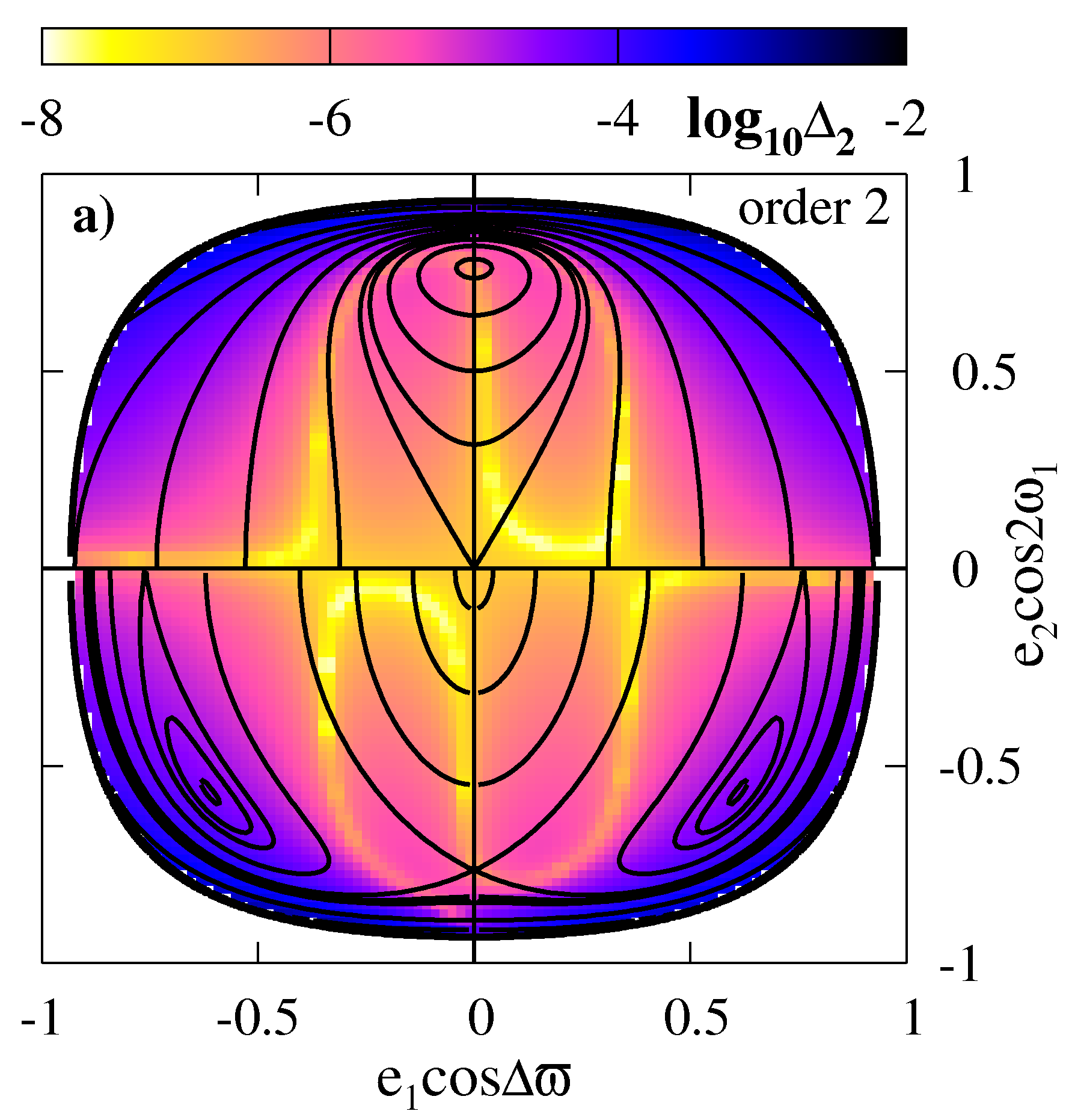
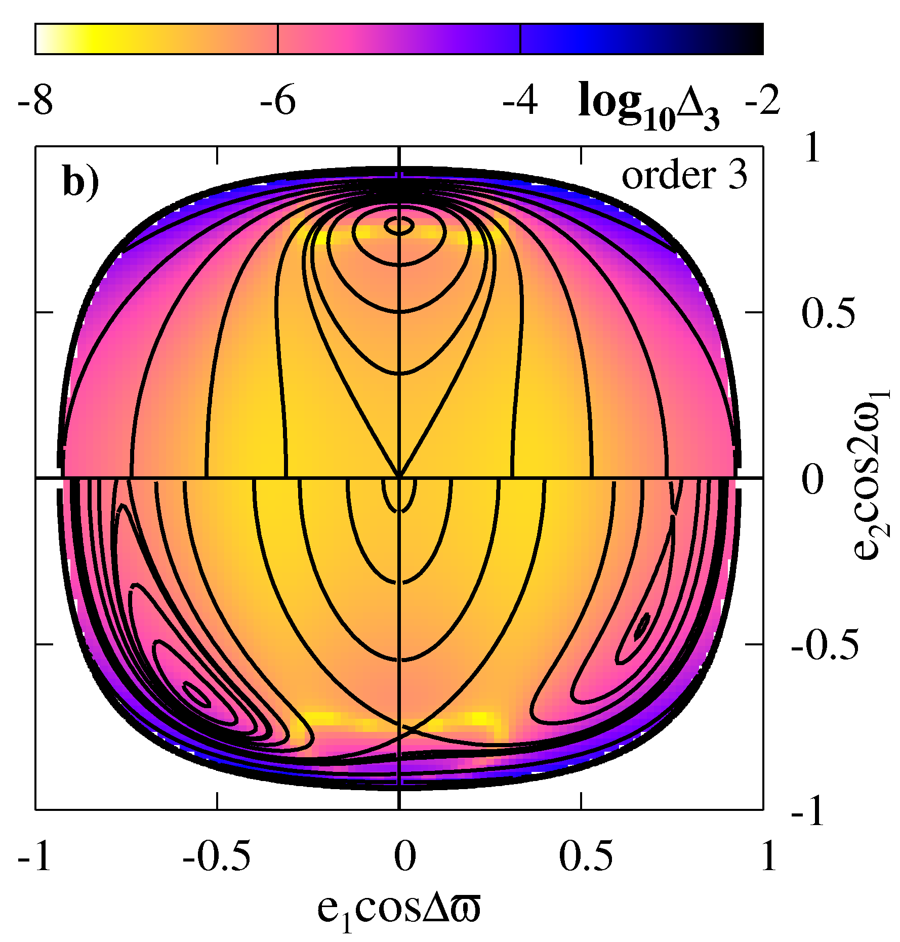
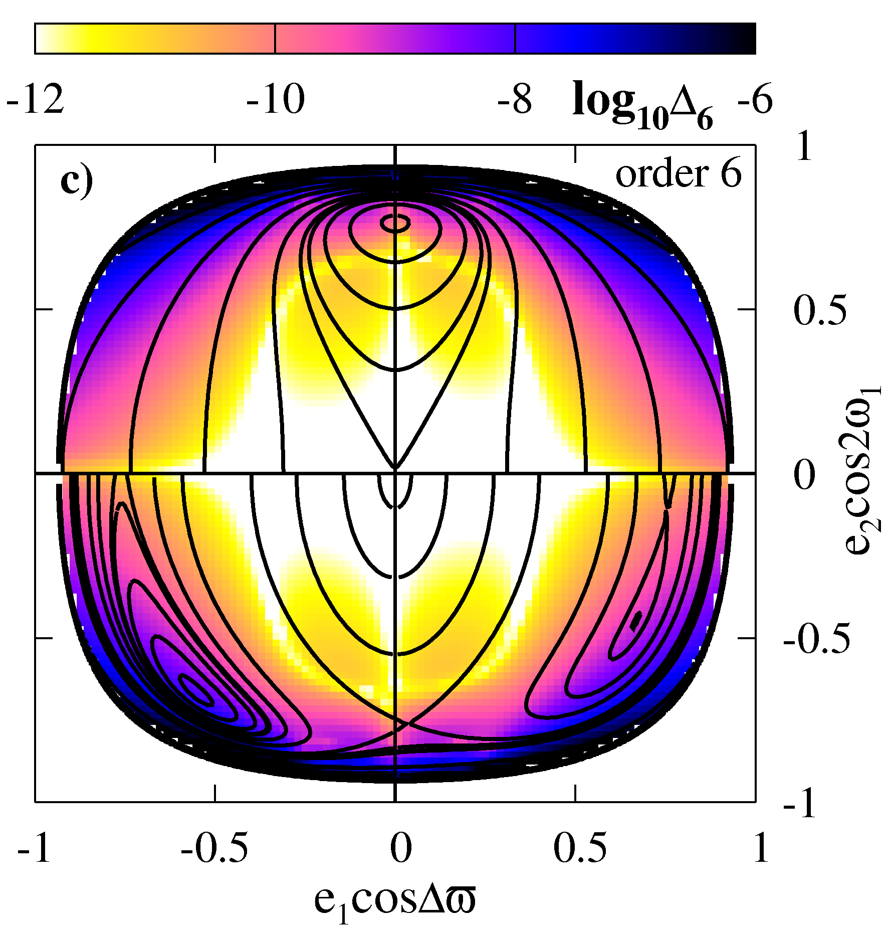
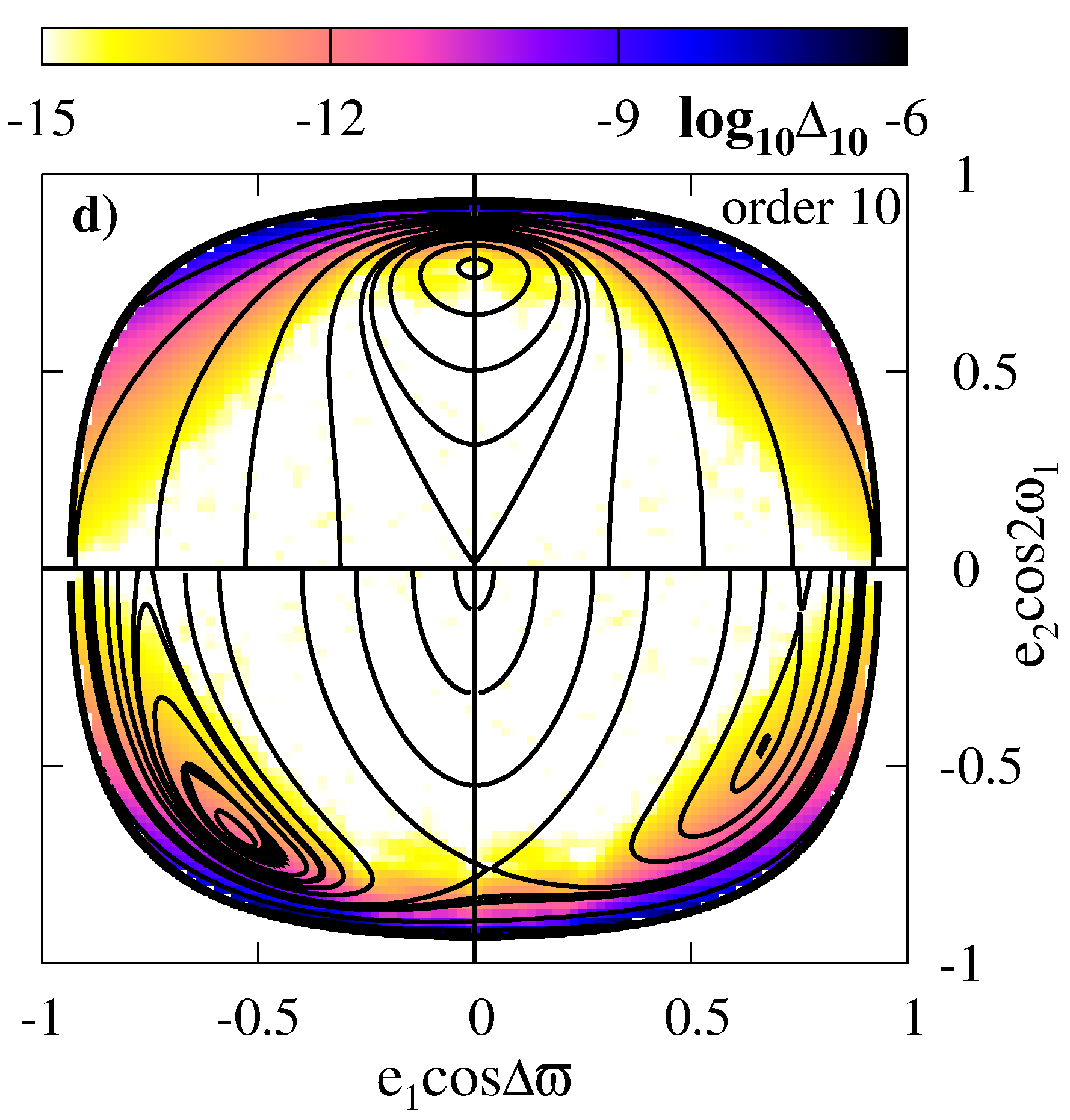
An inspection of Fig. 1 reveals that the octupole model reconstructs the secular Hamiltonian and its shape in the ${\cal S}$-plane very well, because the largest deviations $\Delta_{3}\sim 10^{-3}$ appear only for $e_{1}\sim 1$. In other parts of the representative plane, $\Delta_{3}\sim 10^{-5}$. The high-order expansions are obviously even more precise. Following estimates of the secular frequencies in the relevant parameter ranges (see Sect. 3), the averaging principle assures us that the orbital evolution of the secular system follows closely the “real” orbits. Hence, we may quite safely skip a comparison of the results from both approaches by direct numerical integrations.

The octupole model introduces the first order perturbation to the integrable quadrupole model, hence, because it is very precise in the range of small $\alpha$, we further focus on this most simple, non-trivial case.

3.3 Equilibria in the secular 3D problem

In this work, we focus on the simplest class of solutions that are the equilibria (or stationary solutions). These solutions imply the basic structure of the phase space. By determining their stability, we may derive the local structure of neighboring phase trajectories through relatively simple analysis. The equilibria of the non-resonant system in terms of the quadrupole approximations were studied in the past, (e.g., Krasinskii, 1974; Lidov & Ziglin, 1976). In our earlier work (Migaszewski & Goździewski, 2009a), we classified families of equilibria emerging in the two-planet, non-planar problem, in terms of the quasi-analytic averaging, and basically exact secular model. We studied a few families of equilibria known in the literature, e.g., the zero-eccentricity solutions and the Lidov-Kozai resonance. We also found new families of these equilibria, in particular, the so called chained orbits solution that could be hardly derived with the perturbative approach, although the results in Gronchi & Milani (1998) might be applied here. This work focus on the planetary regime of parameters $\mu,\alpha$, the mass ratio $\mu$ was restricted to the range of $[0.1,2]$ and $\alpha\in[0.1,0.667]$. Moreover, we explored the whole permitted range of $\mathcal{A}\in[0,1]$. Yet we learned that the semi-analytic approach has serious disadvantages. All calculations, including the integrations of the equations of motions, and the stability analysis must be performed with the help of numerical algorithms. This may introduce large errors and hinders the analytic, qualitative analysis of the problem.

In this section, we extend the study of stationary solutions in (Migaszewski & Goździewski, 2009a) to a wider range of the mass ratio, $\mu>2$. Simultaneously, we consider smaller $\alpha<0.1$. That makes it possible to apply the analytic model described and tested in Sect. 3. Because planets emerge most likely from remnants of a thin protoplanetary disk, we also restrict our attention to mutual inclinations up to $i_{{\mbox{\scriptsize mut}}}\sim 90^{\circ}$ (direct orbits). In that range, we may find families of equilibria related to the zero-eccentricity orbits, and the LK resonance classified in (Migaszewski & Goździewski, 2009a) as solutions of family IVa, accompanied by families IIIa, IIIb, and IVb+. Our analysis is also restricted to the initial conditions in quarters III and IV of the ${\cal S}$ -plane, in which these solutions may only “reside”. This region of the parameter space has been studied (e.g., Krasinskii, 1974) with the quadrupole-level model which is somehow the next to trivial, non-interacting Keplerian approximation of the three-body orbits. However, as we show below, this approximation may introduce artifacts due to generally non-realistic symmetry of the secular Hamiltonian. Obviously, to avoid this problem, higher order expansions are required. We also attempt to extend the results of Ford et al. (2000), who applied the octupole-level theory to the analysis of hierarchical planetary systems with very small $\alpha\sim 0.01$.

           

Figure 2: Levels of $\mathcal{H}_{{\mbox{\scriptsize sec}}}$ at the ${\cal P}_{S}$-plane calculated for $\alpha=0.01$ and $\mu=20$. Panels from a) to f) are for different values of $\mathcal{A}=\{0.08,0.12,0.16,0.19,0.2,0.25\}$, respectively. These values of $\mathcal{A}$ imply the mutual inclination at the origin $i_{0}=\{49^{\circ},61^{\circ},70^{\circ},{\color[rgb]{0,0,0}77^{\circ}},79^{\circ},{\color[rgb]{0,0,0}89^{\circ}}\}$, respectively. The intensity of shaded ares encodes the mutual inclination in prescribed ranges, darker shade is for larger $i_{{\mbox{\scriptsize mut}}}$. The inclinations ranges are $i_{{\mbox{\scriptsize mut}}}=(35^{\circ},45^{\circ}),(40^{\circ},55^{\circ}),(50^{\circ},65^{\circ}),{\color[rgb]{0,0,0}(60^{\circ},75^{\circ})},(60^{\circ},75^{\circ}),{\color[rgb]{0,0,0}(70^{\circ},85^{\circ})}$ in subsequent panels.

Figure 3: Families of stationary solutions (IVa, IIIa, IIIb, IVb+). Semi-major axes ratio $\alpha=0.01$, mass ratio $\mu=20$. Dark dots are for stable equilibria, grey dots are for unstable equilibria. Crossed and dotted circles mark bifurcations. Small arrows shows the direction of particular stationary solution with increasing $\mathcal{A}$. Green dots are for the positions of equilibria for particular values of $\mathcal{A}=0.12,0.16,0.19,0.2,0.25$ (the energy levels are shown in Fig. 2). Solutions are for classic model, and were obtained with the help of the octupole theory.

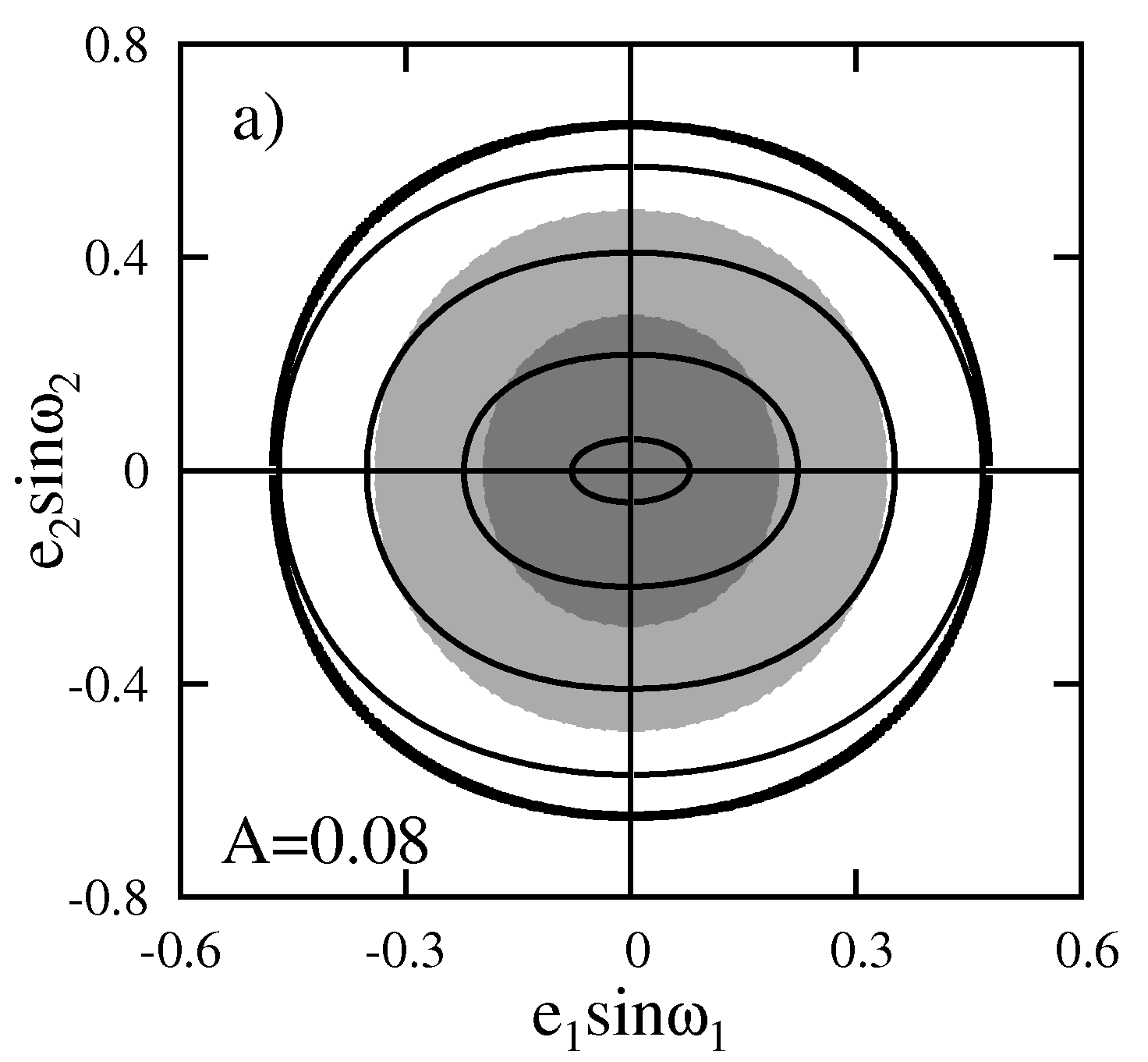
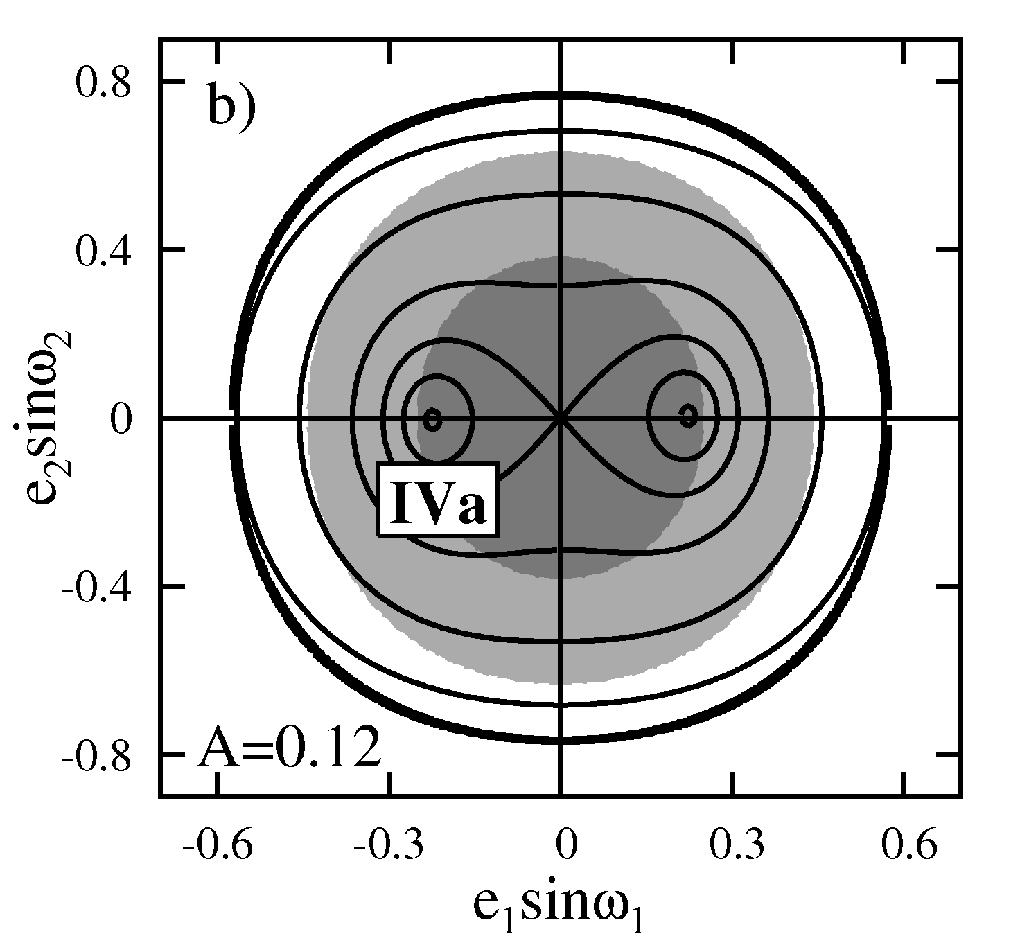
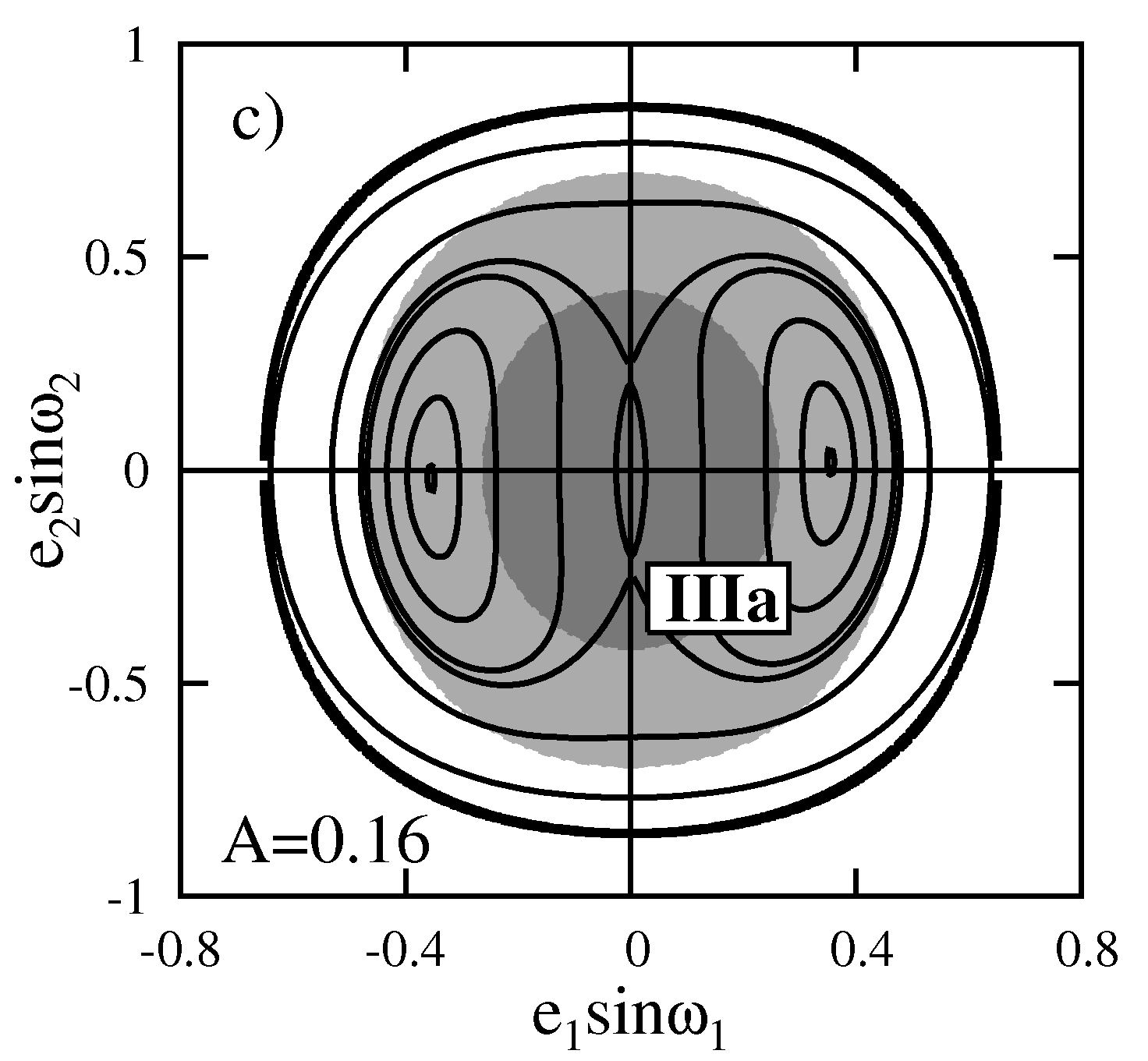
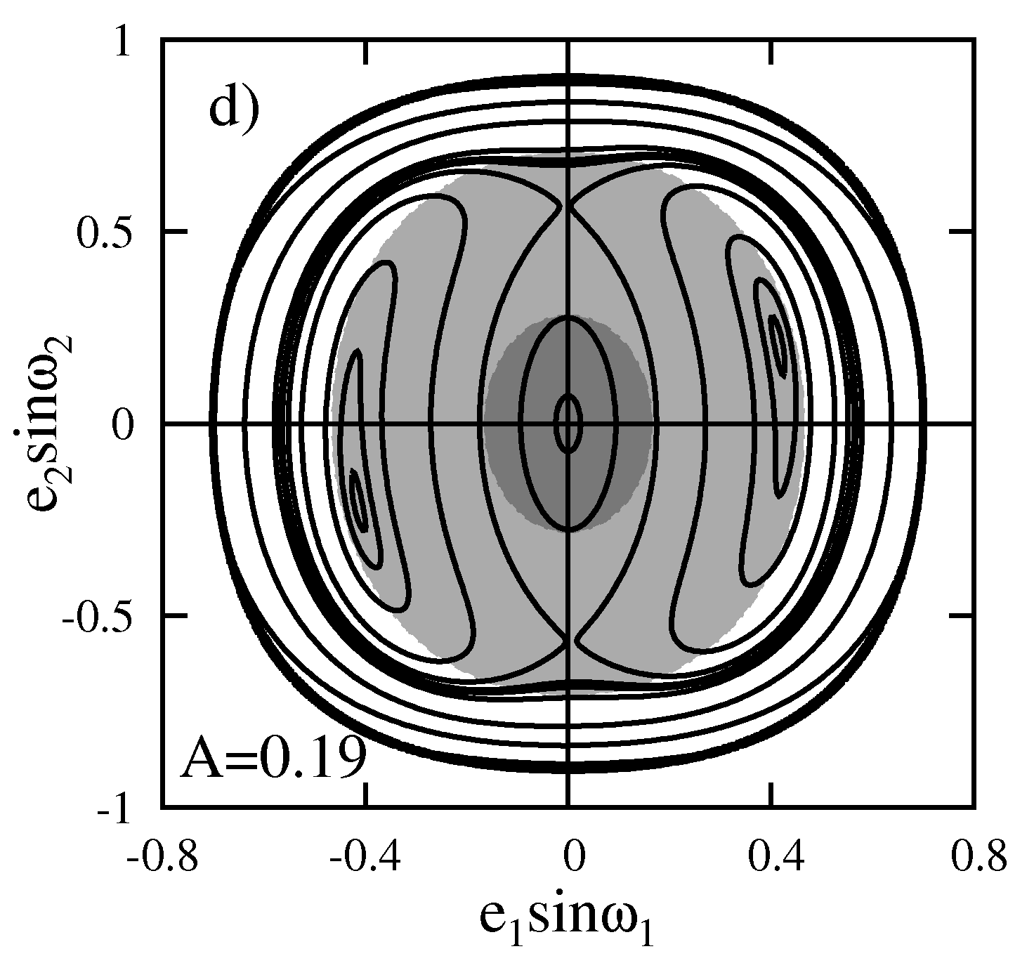
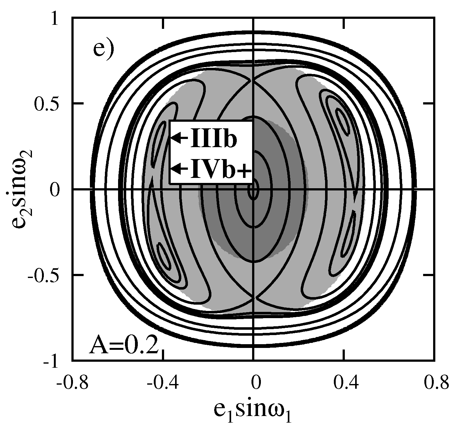
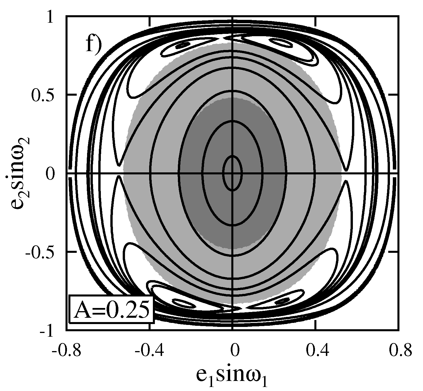
To show the generic properties of the relevant families of equilibria, we begin with an example that is illustrated in Figure 2. Panels in this figure show levels of $\mathcal{H}_{{\mbox{\scriptsize sec}}}$ at the ${\cal P}_{S}$-plane for $\alpha=0.01$ and $\mu=20$ and a few different values of $\mathcal{A}$. Panel 2a was derived for $\mathcal{A}=0.08$, and it reveals the zero-eccentricity equilibrium. For larger $\mathcal{A}=0.12$ (Fig. 2b) the figure-eight structure of Lidov–Kozai equilibrium appears, and is labeled with IVa. We recall, that the mutual inclination of circular orbits that corresponds to the LK bifurcation will be called the critical inclination, $i_{{\mbox{\scriptsize crit}}}$ although, in general, any such value of the mutual inclination that leads to a bifurcation of equilibria has the sense of being “critical” (Krasinskii, 1972, 1974). For larger value of $\mathcal{A}=0.16$ (Fig. 2c) the LKR “moves” towards larger $e_{1}$ (simultaneously, $e_{2}\sim 0$ ) and a new saddle point appears. We call this solution a member of family IIIa. For larger $\mathcal{A}=0.19$ (Fig. 2d), these structures still expand, and for $\mathcal{A}=0.2$ (Fig. 2e) two new equilibria emerge: one is associated with quasi-elliptic point (family IIIb from hereafter), and a saddle of family IVb+. Apparently, it emerges from a point near the IVa solution in the ${\cal P}_{S}$-plane, nevertheless it does not correspond to a bifurcation of this equilibrium, see (Migaszewski & Goździewski, 2009a). Solution IVa moves towards larger $e_{2}$, see Fig. 2f).

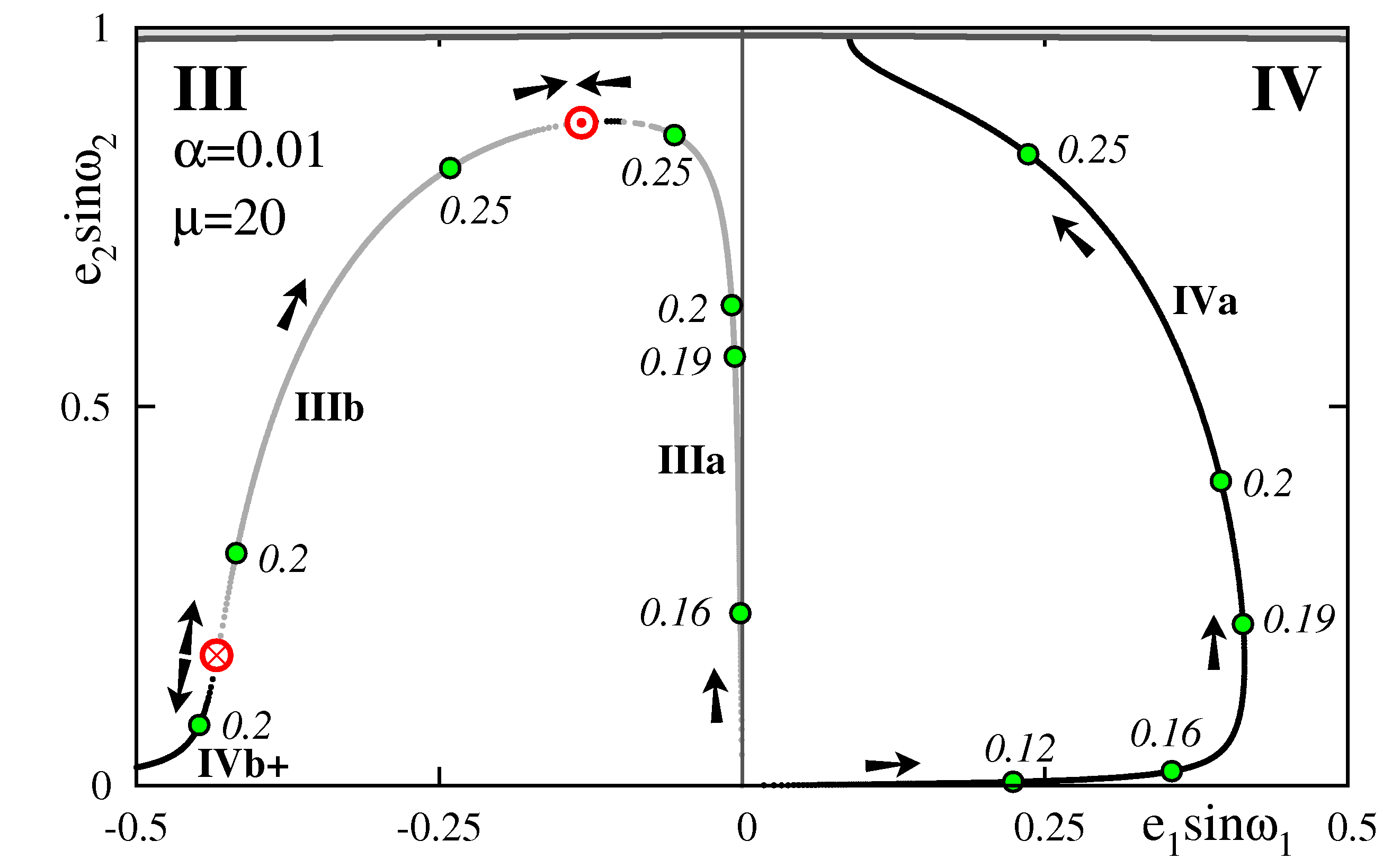
The parametric paths of these equilibria in terms of $\mathcal{A}{}$, may be depicted in the ${\cal P}_{S}$-plane (Fig. 3). Black and grey curves are for the stable and unstable equilibria, respectively. The relevant families of equilibria are labeled with Roman numbers and Latin letters. The direction of “motion” of particular solutions along the $\mathcal{A}$-axis is marked with arrows. For a reference, positions of the equilibria for a few discrete values of $\mathcal{A}=0.12,0.16,0.19,0.2,0.25$ (corresponding to subsequent panels in Fig. 2), are marked with green dots and labeled. Following a particular evolution path of equilibrium IVa, we see that it appears for $\mathcal{A}\sim 0.1$ through a bifurcation of the origin. When $\mathcal{A}$ increases, this solution moves along $e_{2}\sim 0$ towards larger $e_{1}$. For $\mathcal{A}\sim 0.17$, it reaches the maximal $e_{1}\sim 0.4$, and it turns back, towards smaller $e_{1}$ with simultaneous increase of $e_{2}$. When $\mathcal{A}$ increases even more, this solution reaches the border of convergence of the analytic expansion. We call that border the anti-collision line [see (Migaszewski & Goździewski, 2008)].

The parametric evolution of equilibria in quadrant III is more complex. The first non-trivial stationary solution appears for $\mathcal{A}\sim 0.15$, which is unstable, saddle point IIIa. It evolves along $e_{1}\sim 0$ and then $e_{2}$ increases to large values. For $\mathcal{A}\sim 0.195$, two new solutions IIIb and IVb+ emerge from the elliptic structure related to the LKR (see Fig. 2e). One of them is stable (solution IVb+) and the another one is unstable (solution IIIb). They appear around $(e_{1}\sim 0.45,e_{2}\sim 0.15)$ . When $\mathcal{A}$ increases, the solution IVb+ moves towards $e_{1}\rightarrow 1$ and $e_{2}\rightarrow 0$. Simultaneously, equilibrium IIIb is shifted towards increasing $e_{2}$ and decreasing $e_{1}$. Then also IIIa increases $e_{2}$ and leaves off the $e_{1}=0$ axis. Finally, for $\mathcal{A}\sim 0.26$, equilibria IIIa and IIIb merge at one point $(e_{1}\sim 0.13,e_{2}\sim 0.8)$.

4 The secular chaos

Following (Michtchenko et al., 2006), we shown in (Migaszewski & Goździewski, 2009a) that the averaged 3D model may involve strongly chaotic motions, in the secular time-scale. To study in details, how the model parameters influence the structure of the ${\cal S}$-plane, and how it relates to the long-term chaotic phenomena, we apply the fast indicator approach. Among many numerical tools of this kind, we choose the so called coefficient of the diffusion of fundamental frequencies $\sigma$ introduced by (Laskar, 1990). To check whether a phase space trajectory of a quasi-integrable Hamiltonian system is regular (quasi-periodic) or irregular (chaotic), one integrates the equations of motion over two subsequent intervals of time, e.g., $[0,T]$ and $[T,2T]$. Next, we resolve the frequencies in the discrete orbital signal with the help of refined FFT analysis (Laskar, 1990), obtaining two estimates of a given frequency, say $f_{T}$ and $f_{2T}$, over these two intervals of time. The coefficient of the diffusion of the fundamental frequency is then defined through:

$$\sigma=\left\|\frac{f_{T}}{f_{2T}}-1\right\|.$$

Clearly, if the signal does not change over time, $\sigma\sim 0$ and this means that the phase trajectory is quasi-periodic (stable). If $\sigma$ is significantly different from 0, the trajectory is chaotic and regarded unstable. In our calculations, we used a variant of the frequency analysis developed by (Šidlichovský & Nesvorný, 1996), which is called the Frequency Modified Fourier Transform (FMFT). We also used publicly available code of the FMFT algorithm, kindly provided by David Nesvorný on his personal web-page.

Because the secular evolution is associated with $\omega_{i}$ angles, we compute the $\sigma$ coefficient on the basis of complex time-series $\{G_{i}(t)\exp\mbox{i}\omega_{i}(t)\},\ldots i=1,2,$ where i is the imaginary unit. In this signal, the osculating eccentricity and pericenter argument for each planet represent rescaled canonical action-angle variables. Hence, resolving its Fourier components, we may determine the leading amplitudes (proper eccentricities) and the fundamental frequencies of pericenter angles.

Next, we did massive integrations of the secular equations of motion. The initial conditions were selected at the grid of $200\times 100$ data points of the ${\cal P}_{S}$-plane. At each point of the dynamical map, we integrated the secular trajectory over $\sim 10^{4}$ secular periods with respect to the smaller frequency (typically, one of the fundamental frequencies is much larger than the other one). Having the computed phase trajectory, we then find an estimate $\sigma$, as well as the maximal eccentricities attained by both orbits during the integration time (the so called $\max e$ indicator) as well as the amplitude of variation of the mutual inclination $\Delta i\equiv(\max i_{{\mbox{\scriptsize mut}}}-\min i_{{\mbox{\scriptsize mut}}})$ attained during the integration time. These geometrical characteristics are very useful to understand the source of instabilities indicated and detected by the diffusion coefficient $\sigma$.

     

Figure 4: Dynamical maps for the classic (point-mass Newtonian) model, shown in the ${\cal P}_{S}$-plane. Panels from a) to d) are for the coefficient of the diffusion of fundamental frequencies ($\sigma$), maximal eccentricity of the inner and outer planet ($\max e_{1},\max e_{2}$), respectively, and the amplitude of variation of the mutual inclination ($\Delta i$). Dots mark areas of librations of $\omega_{1}$ (panel b), $\omega_{2}$ (panel c), and $\Delta\varpi$ (panel d). Stationary solutions are marked with circles: dotted circles are for stable equilibria (corresponding to the maximum of the secular Hamiltonian), crossed circles are for unstable equilibria, empty circles are for the linearly stable equilibria. These solutions are labeled, in accord with (Migaszewski & Goździewski, 2009a). Parameters of the system: $\alpha=0.01,\mu=20,\mathcal{A}=0.12$, see also Fig. 2b.

     

Figure 5: Dynamical maps for the Newtonian, point mass model in the ${\cal P}_{S}$-plane, $\mathcal{A}=0.16$. See the caption to Fig. 4 for more details, and also Fig. 2c.

     

Figure 6: Dynamical maps for the Newtonian, point-mass model, in the ${\cal P}_{S}$-plane, $\mathcal{A}=0.20$. See the caption to Fig. 4 for more details, also Fig. 2e.

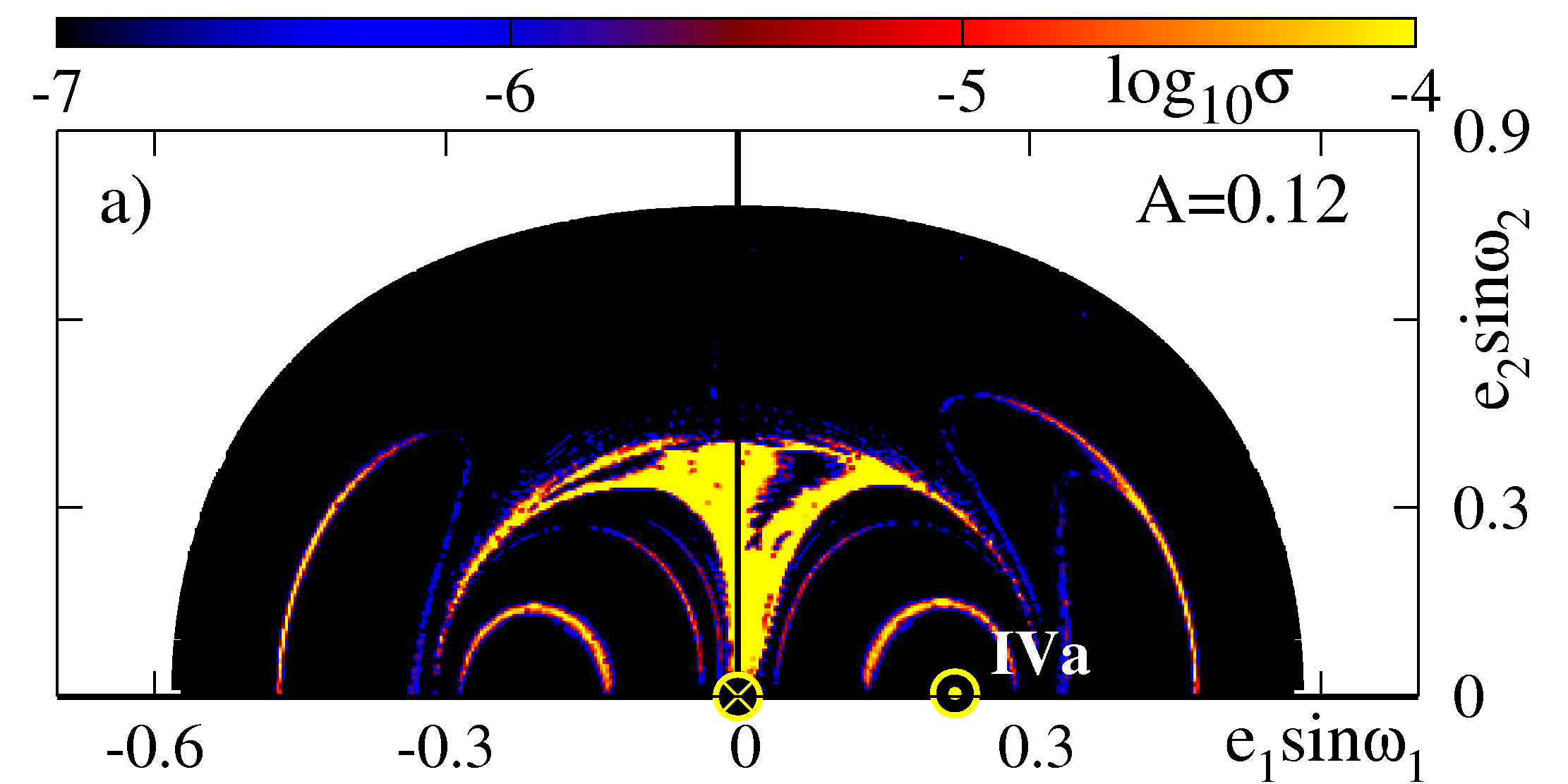
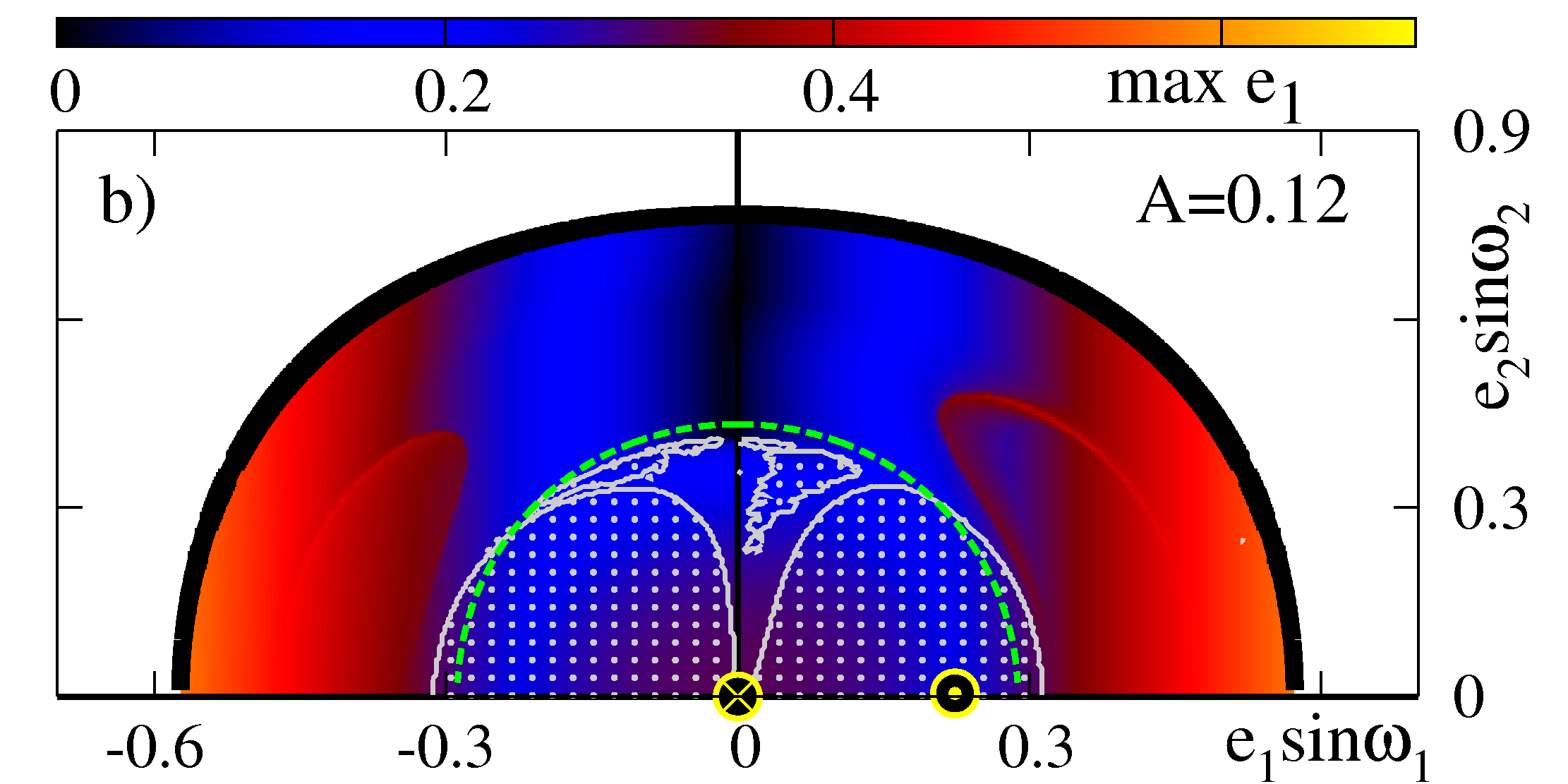
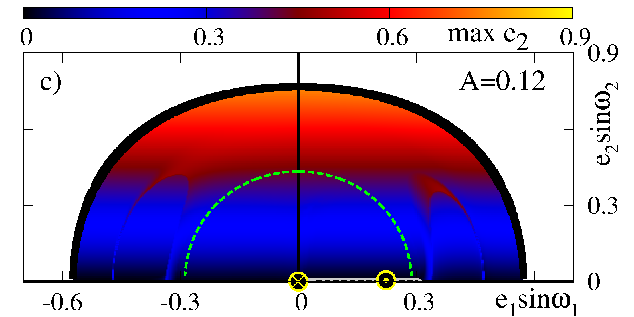
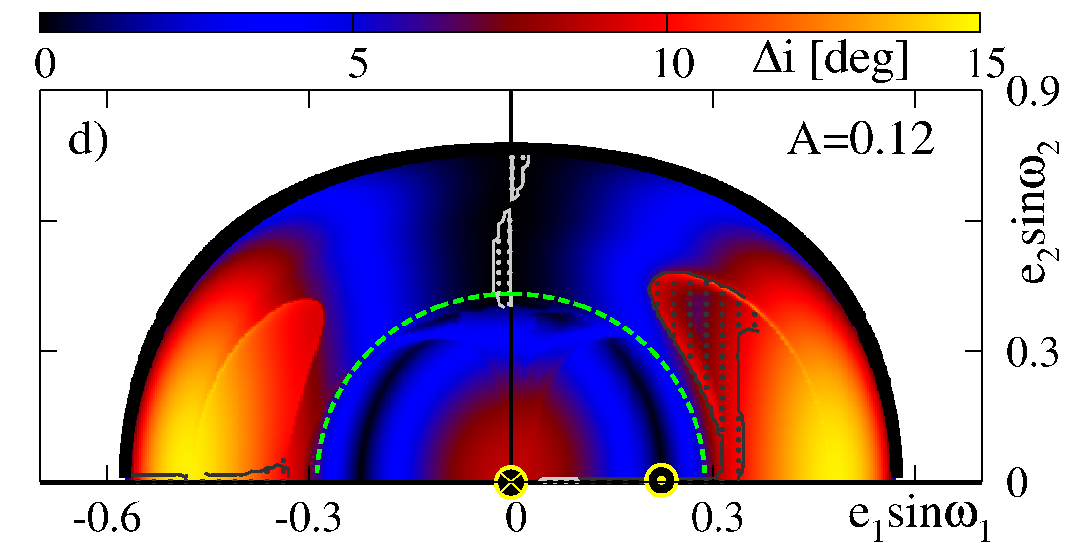
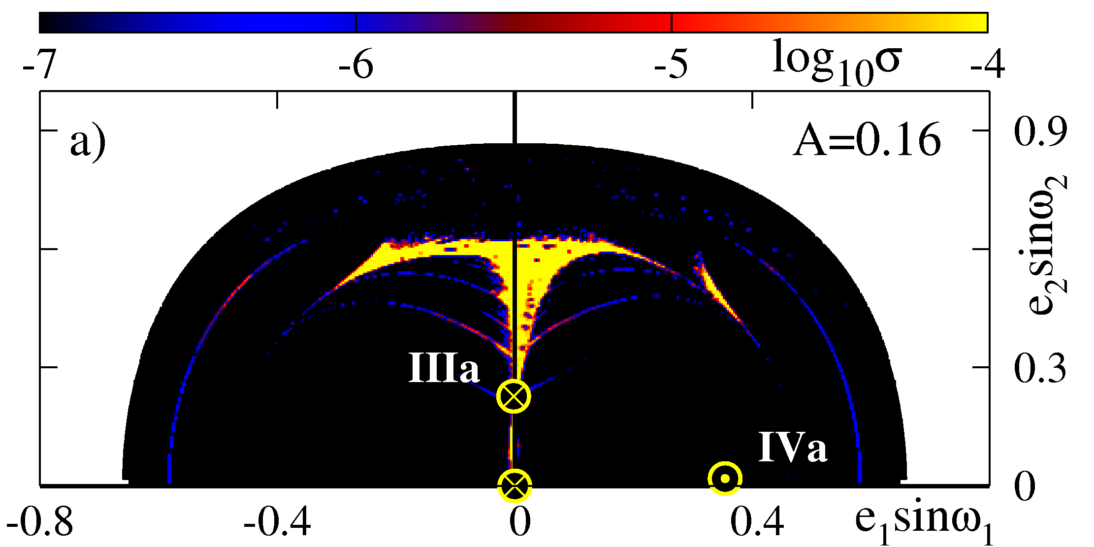
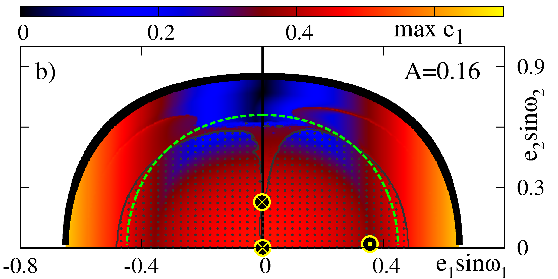
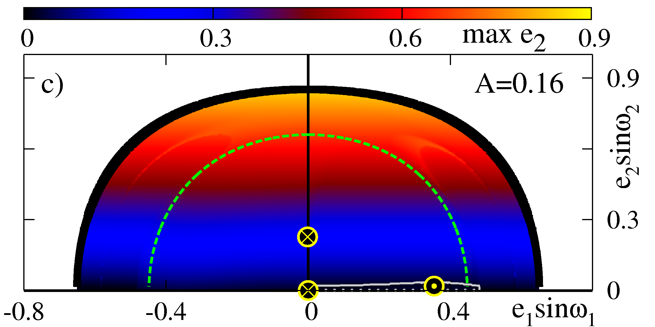
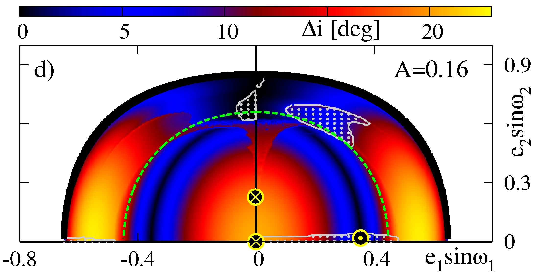
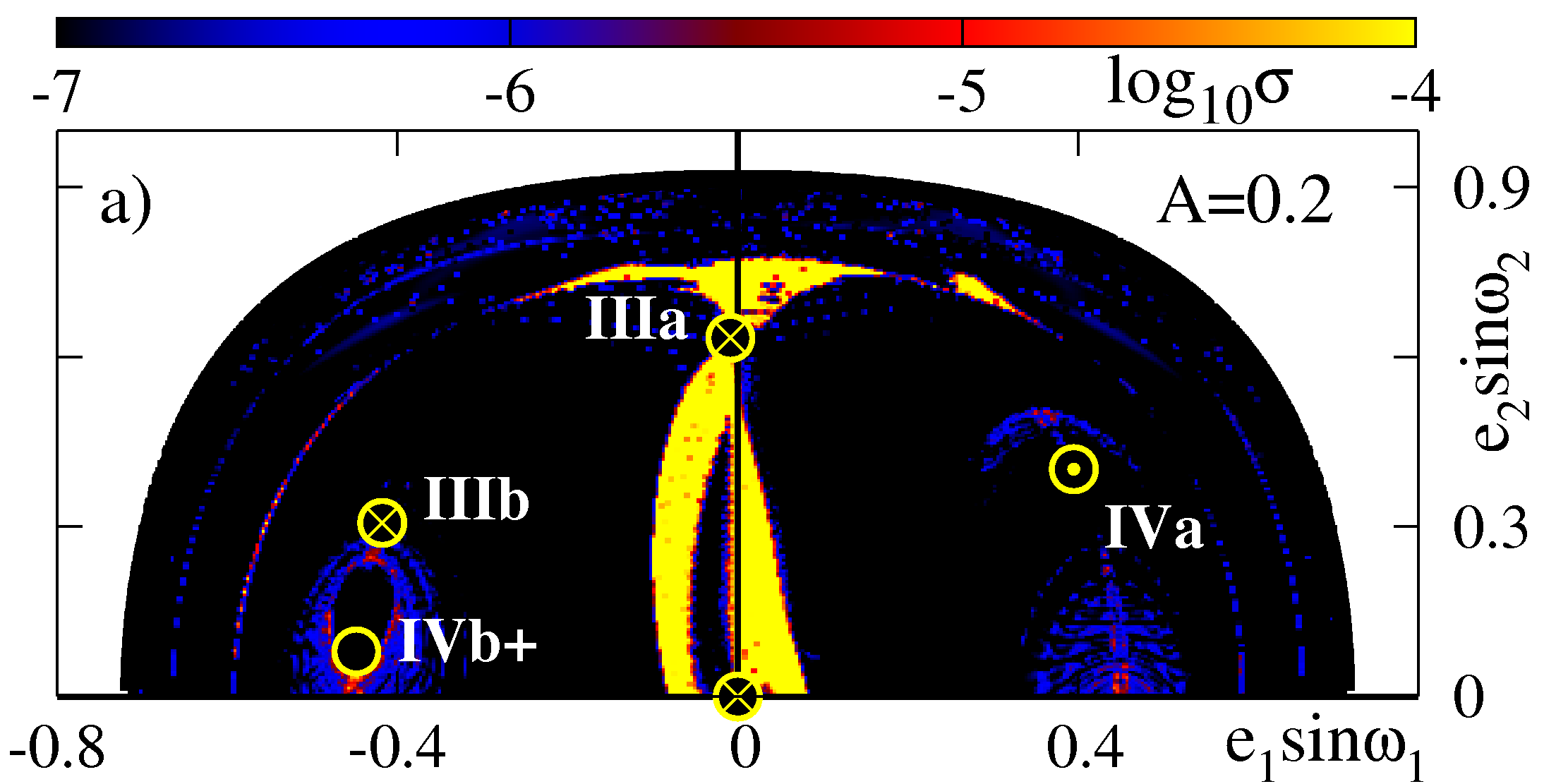
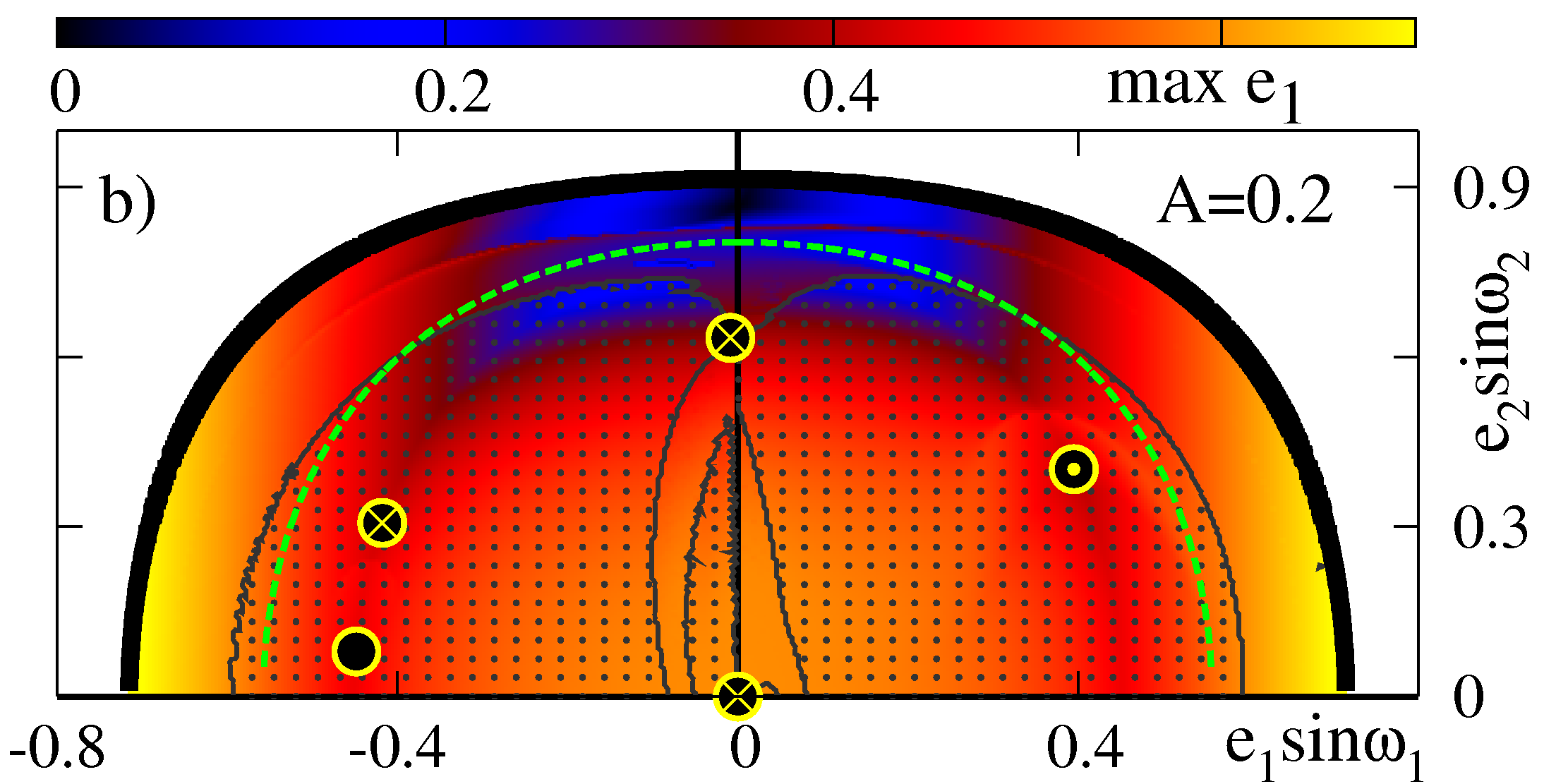
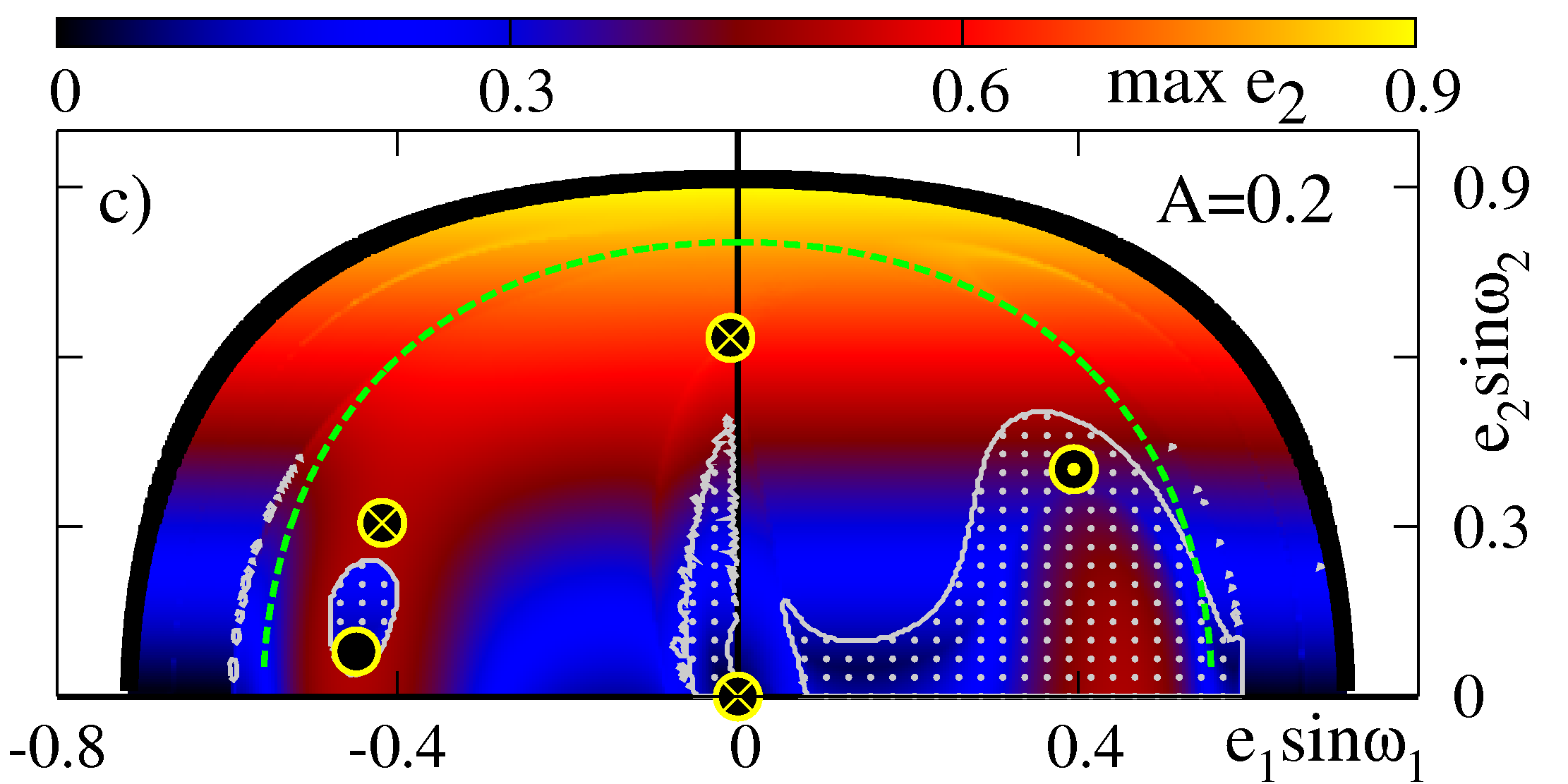
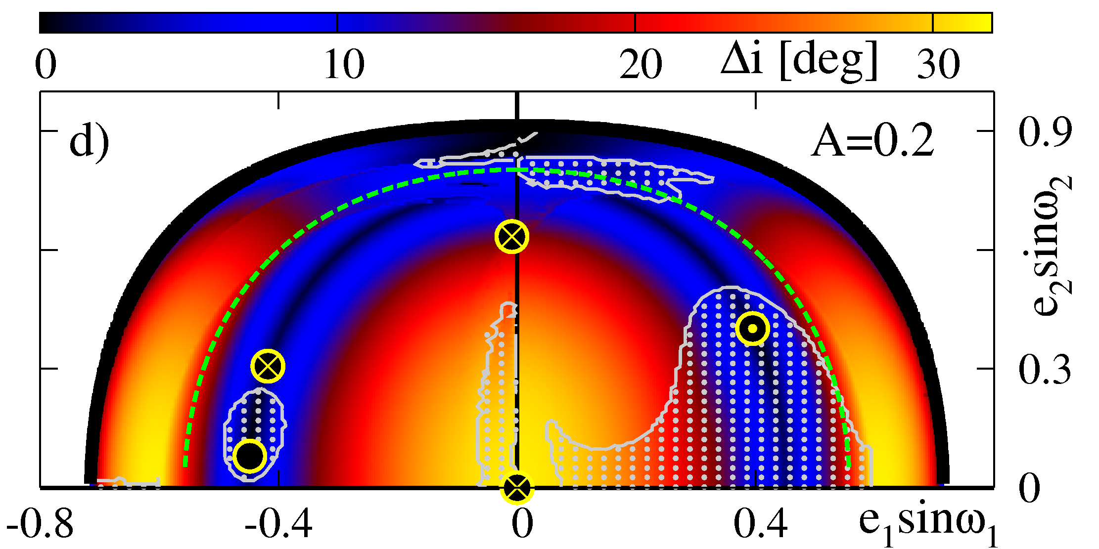
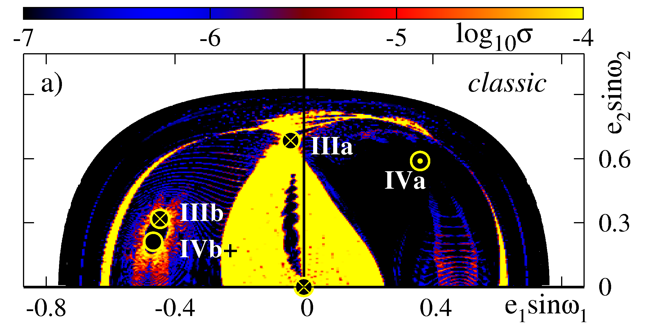
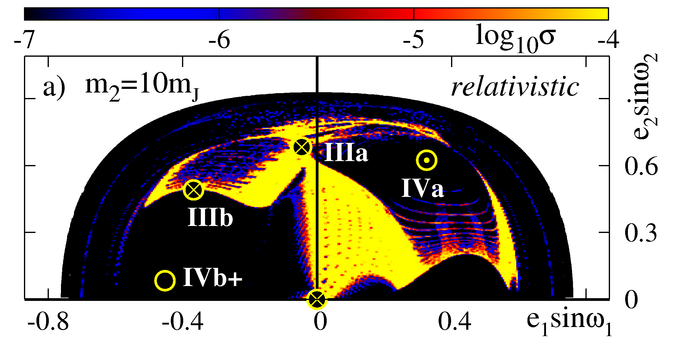
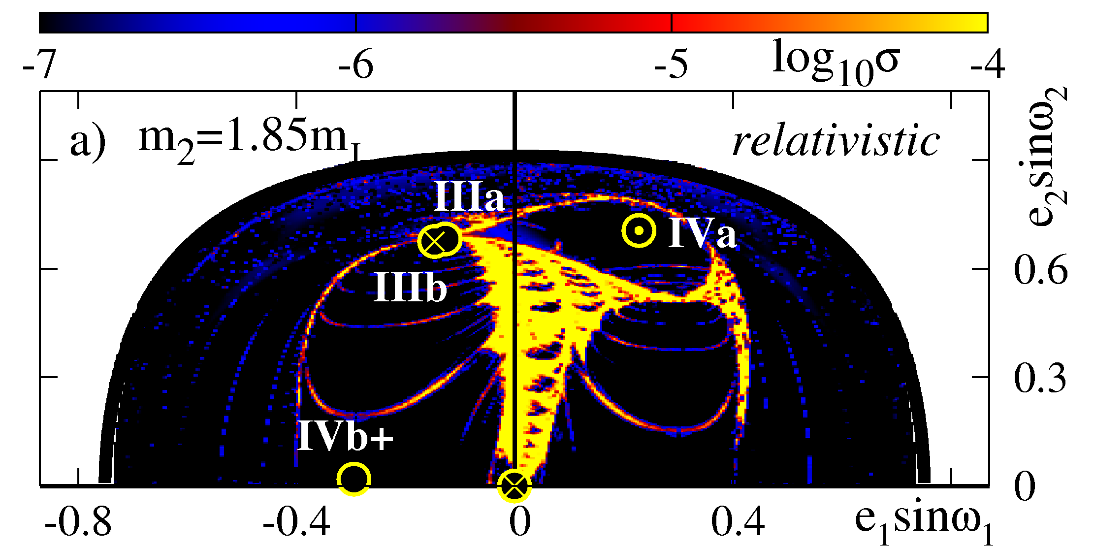
Figures 4–6 illustrate the results derived for the same system that energy levels are shown in Fig. 2. Subsequent figures are for $\mathcal{A}=0.12,0.16,0.2$, respectively (see Figs. 2b,c,e for the respective levels of $\mathcal{H}_{{\mbox{\scriptsize sec}}}$). (We note, that for $\mathcal{A}=0.08$ the view of the phase space is basically very simple and the motions are regular everywhere). The right-hand panel of each figure is for $\sigma$. The dynamical character of the phase-space trajectories is color-coded: black color means quasi-regular evolution of the secular system ($\sigma\sim 10^{-6}$–$10^{-8}$), and yellow colour is for strongly chaotic motions ($\sigma\geq 10^{-4}$). The $\sigma$-maps reveals that almost the whole phase space is filled up with regular motions, and chaos appears only in some small regions in the ${\cal P}_{S}$-plane. For a reference, the coordinates of equilibria IVa, IIIa, IIIb, IVb+ and 0 (the equilibrium at the origin) are marked with circles. Dotted circle is for Lyapunov stable solution IVa, crossed circles are for unstable solutions 0, IIIa and IIIb, respectively. Equilibrium IVb+ is linearly stable and is marked with open circle. Clearly, trajectories close to unstable equilibria IIIa and 0 are chaotic. Let us note that unstable equilibrium IIIa lies in a very narrow, chaotic zone too.

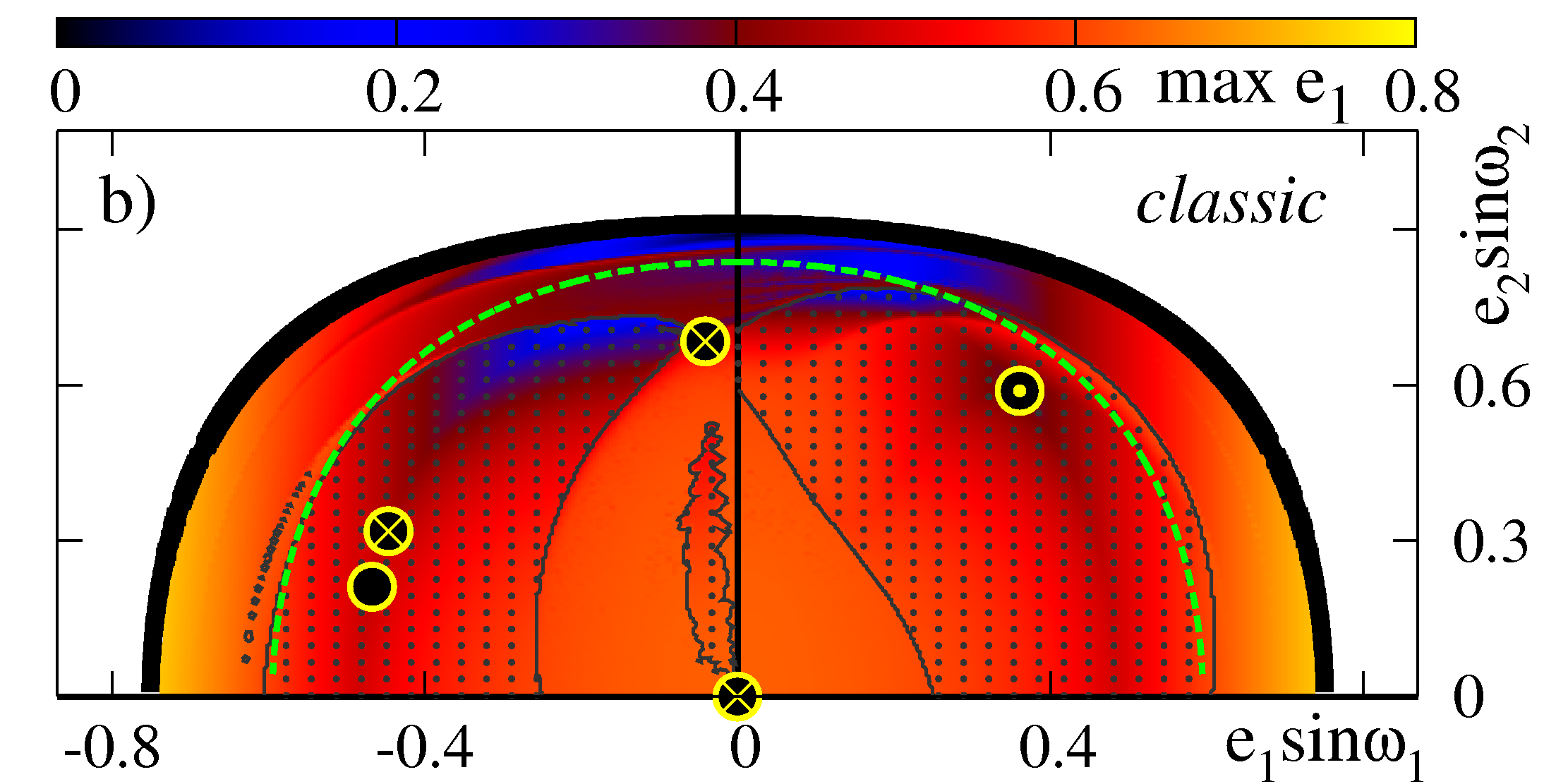
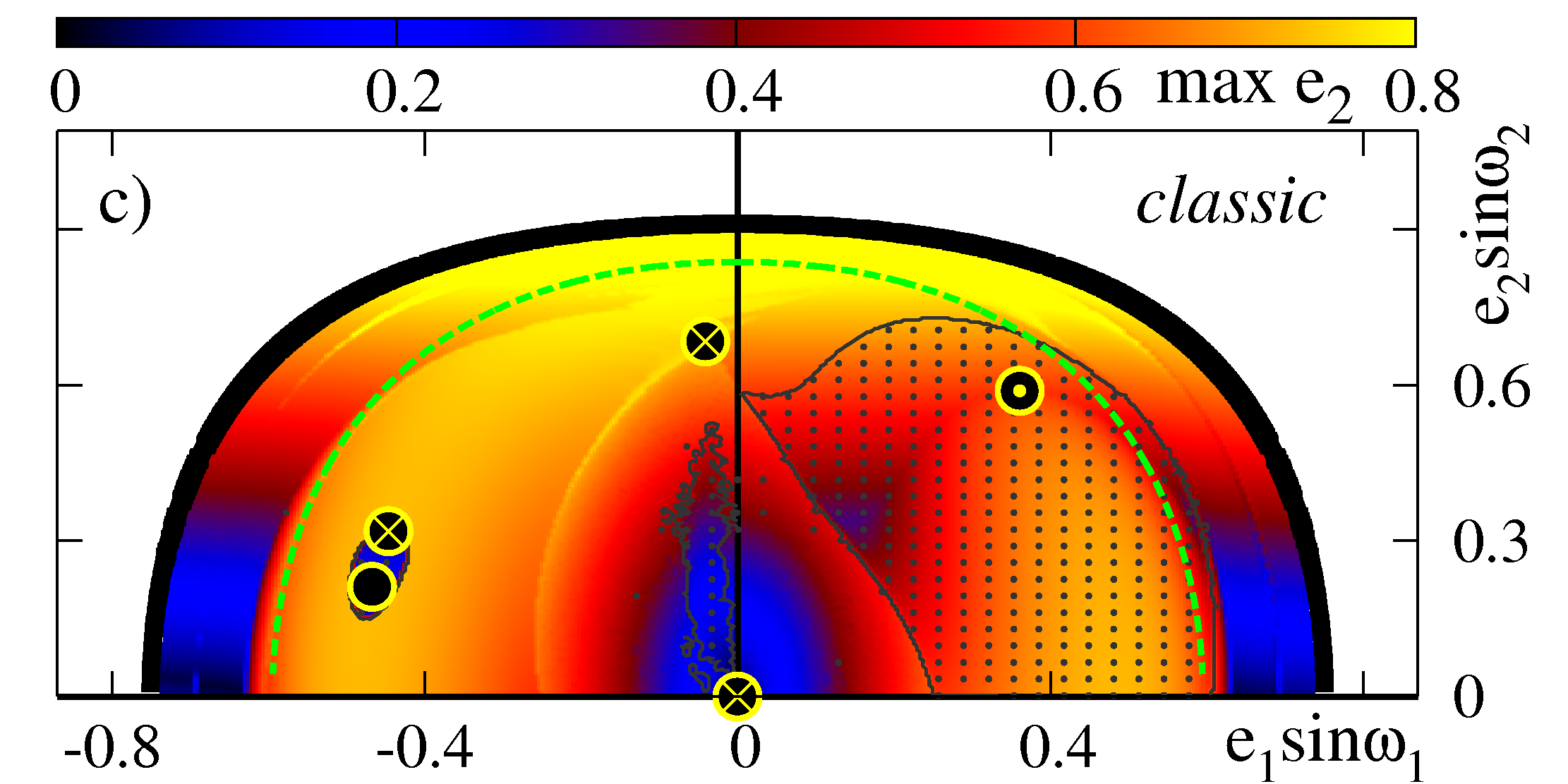
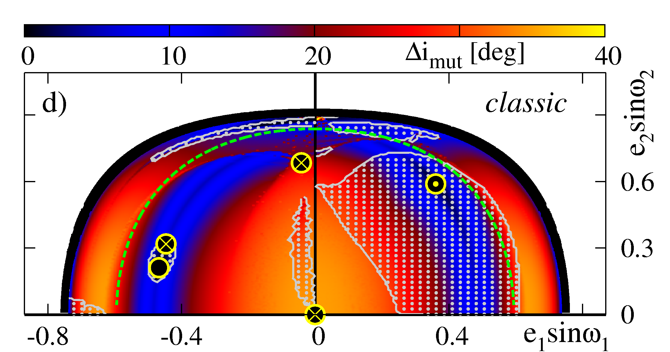
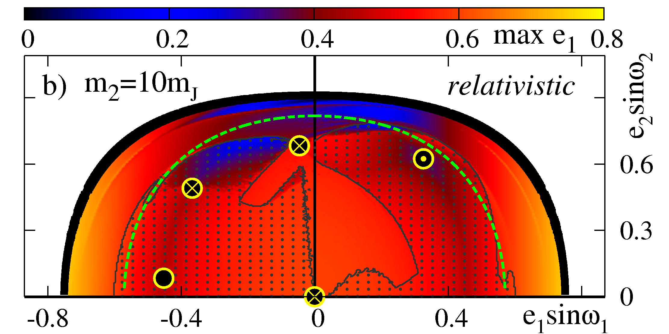
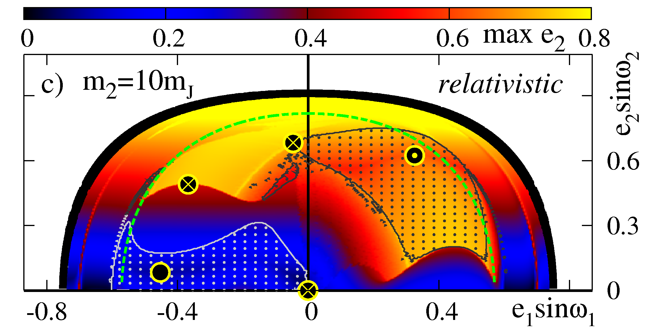
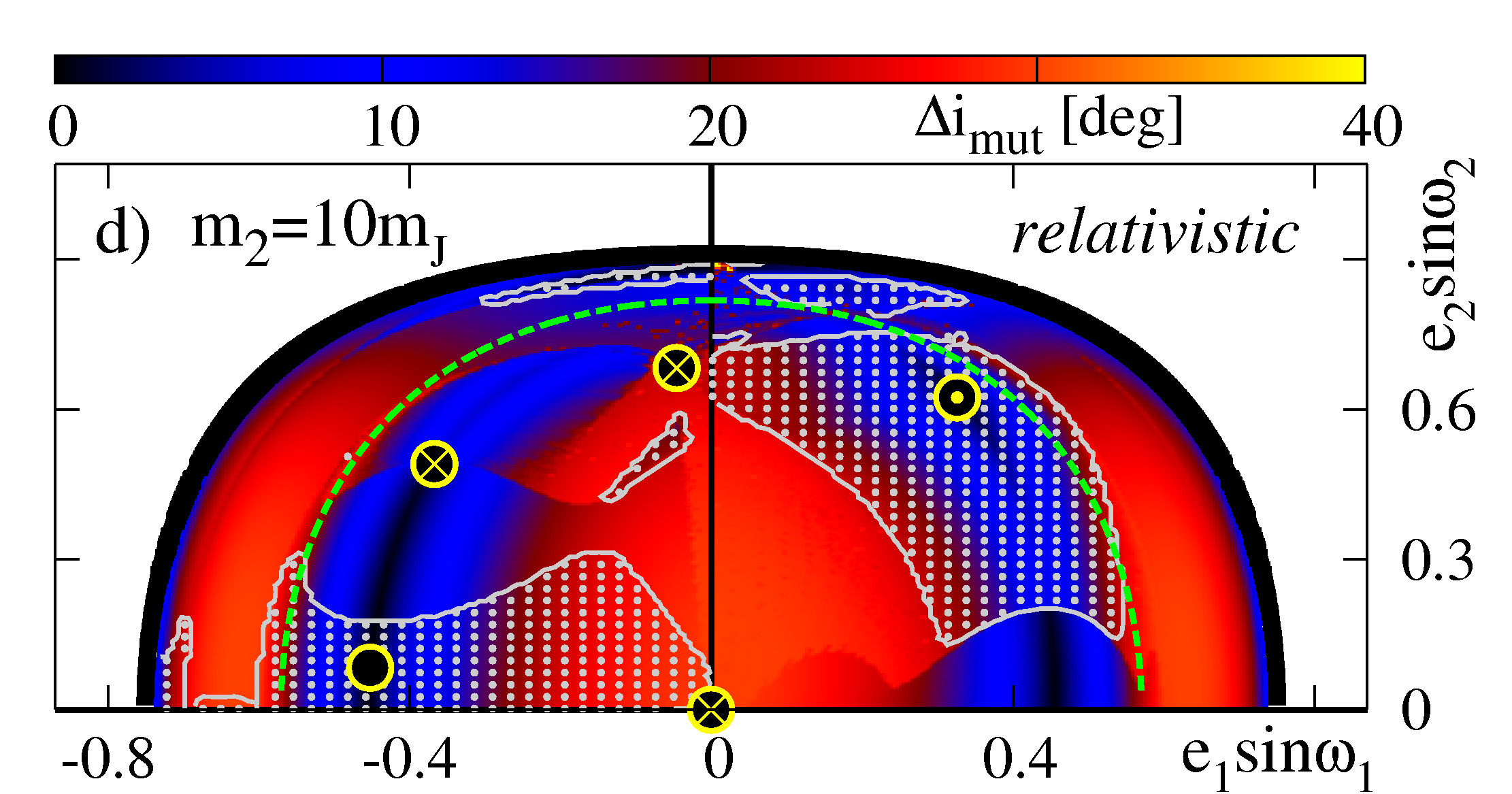
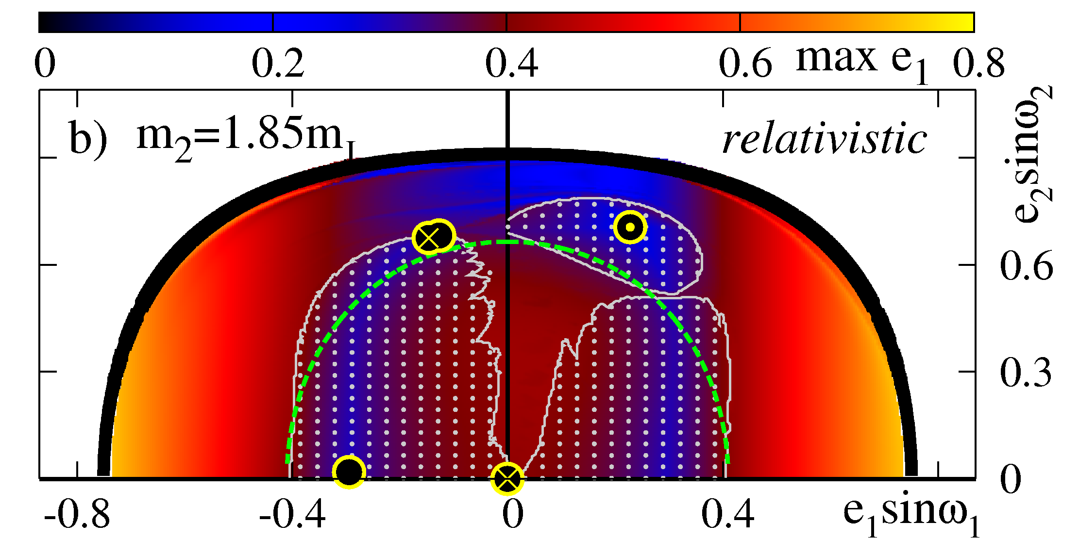
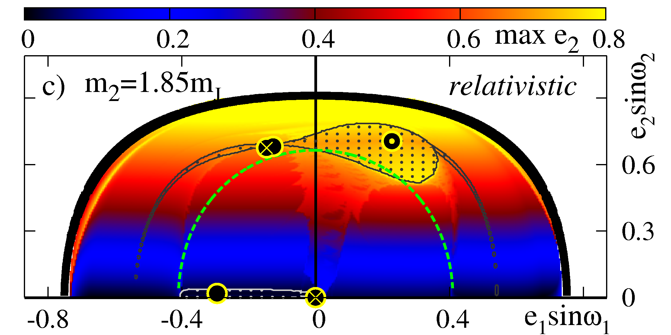
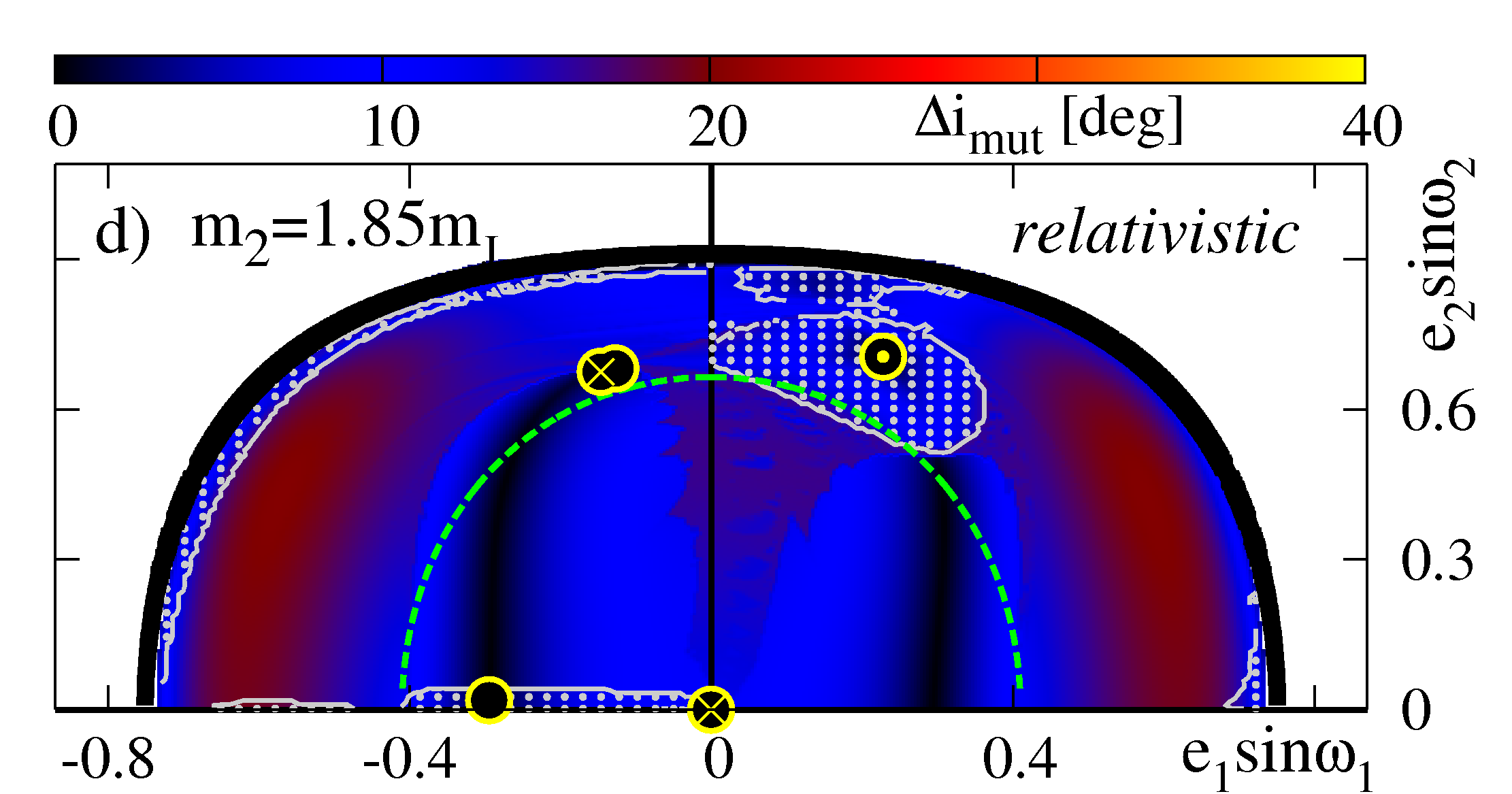
Besides dynamical maps for $\sigma$, Figs. 4–6 illustrate geometric characteristics or orbits in the ${\cal P}_{S}$-plane, in terms of $\max e_{1,2}$ indicator for the inner and the outer orbit, respectively, and for the amplitude of variation of the mutual inclination, $\Delta i$. In all these dynamical maps, the green dashed contours mark the mutual inclination equal to the critical inclination of the LKR bifurcation (Krasinskii, 1972, 1974). Also regions, in which the secular angles $\omega_{1}$, $\omega_{2}$, and $\Delta\varpi$ oscillate, are shown: the gray/white/black dots surrounded by appropriate curves bound initial conditions that lead to librations of $\omega_{1}$ around $\pm\pi/2$ in the $\max e_{1}$-maps, librations of $\omega_{2}$ around $\pm\pi/2$ in the $\max e_{2}$-maps, and librations $\Delta\varpi$ around $0,\pi$ in the $\Delta i$-maps. We note that $\omega_{1}$ librates in almost all regular trajectories with the initial $i_{{\mbox{\scriptsize mut}}}>i_{{\mbox{\scriptsize crit}}}$ . If this condition of the Lidov-Kozai mechanism is fulfilled then $\omega_{1}$ librates around $\pm\pi/2$. In chaotic zones of the ${\cal S}$-plane, these angles do not oscillate, even if condition $i_{{\mbox{\scriptsize mut}}}>i_{{\mbox{\scriptsize crit}}}$ holds true. Angle $\omega_{2}$ librates around $\pi/2$ only when $e_{2}\sim 0$, for $\mathcal{A}=0.12,0.16$. This region extends significantly for larger $\mathcal{A}=0.2$ . In such a case, there are three zones in which both angles $\omega_{1}$ and $\omega_{2}$ librate: a region connected to equilibrium IVa, the neighborhood of linearly stable solution IVb+, and a region of small $e_{1}$ (though there is no stationary solution associated with these librations). The later area is surrounded by strongly chaotic motions shown in the $\sigma$-plane.

Clearly, the equilibria permitted by relatively large $\mathcal{A}$ affect the secular dynamics, which become very complex. This may be better seen in the $\max e$-maps. Subsequent panels in Figs. 4–6 show that the inner eccentricity may be strongly excited if $i_{{\mbox{\scriptsize mut}}}>i_{{\mbox{\scriptsize crit}}}$. For relatively small $\mathcal{A}=0.12$, the inner orbit, which is initially quasi-circular, becomes moderately eccentric, with $\max e_{1}\sim 0.3$. Note that in this specific case, the inner body is $20$ times more massive then the outer companion. Simultaneously, as Fig. 4 shows, the outer eccentricity $e_{2}$ is not amplified. We may conclude that in the regime of the outer LKR, when the inner body is much more massive than the outer body, the secular evolution may lead to strong perturbations of the inner orbit. Hence, even the mass hierarchy is reversed, a strong excitation of the inner eccentricity is still possible, similarly to the LKR in the restricted problem. This dynamical phenomenon may explain a large eccentricity of the binary, when a distant, low-mass and dark companion cannot be detected due to very long orbital period.

The dynamical maps in Figs. 4–6 reveal some zones, in which the outer eccentricity is strongly amplified. This eccentricity is obviously constant in terms of the quadrupole model. This feature of the octupole model shows that the small perturbation may cause extended, geometric changes of the mean orbits. The amplification of $e_{2}$, with simultaneously almost constant relative inclination, $\Delta i\sim\mbox{const}$ (see Figs. 6c,d) seems appear due to the bifurcation of equilibria IVb+ and IIIb for $\mathcal{A}\sim 0.195$.

4.1 A model explaining the secular chaos

The origin of chaotic secular dynamics may be explained by the presence of separatrices, which encompass different types of motions, librations and rotations of angles $\omega_{1}$, $\omega_{2}$ and $\Delta\varpi$. A classification of these libration modes in the secular problem of two planets modes has been introduced in (Michtchenko et al., 2006). The separatrices appear due to equilibria and periodic solutions in the integrable, or close to integrable secular models, which might be understood as the quadrupole approximation and/or the co-planar configuration.

Here, we found a simple explanation of the mechanism generating chaos, which is in fact the same as in the perturbed pendulum. To show this, let us recall that the expansion of $\mathcal{H}_{{\mbox{\scriptsize sec}}}$ to the second order in $\alpha$ is the celebrated integrable quadrupole-level model. The energy levels of this model are illustrated in Fig. 7a. Because $e_{2}$ is the integral of motion, the representative plane may be constructed similarly to the integrable co-planar problem, S${}^{\prime\prime}\equiv\{e_{1}\cos 2\omega_{1}\times e_{2}$}. In the region marked in green colour, any constant level of $e_{2}$ crosses the energy curve in two turning points limiting the range of variation of $e_{1}$. If the $e_{2}$ level is tangent to the given level of the energy, the dynamics must be then confined to fixed $e_{1}$, hence we obtain an equilibrium point (stable or unstable). A set of these equilibria for increasing, fixed values of $e_{2}$ is marked by two thick curves that meet around of $(e_{1}=0,e_{2}\sim 0.4)$. This is the bifurcation point, at which two families of equilibria emerge — the stable branch of the LKR and the unstable origin $(e_{1}=0,e_{2}=0)$.

For a given value of constant $e_{2}$, we may then find the maximum range of $e_{1}$, which corresponds to librations of the canonical angle $\omega_{1}$, and this value determines the position of separatrix, see Fig. 7b for the separatrix shown in the phase diagram in the $\{e_{1}\cos 2\omega_{1}\times e_{1}\sin 2\omega_{1}\}$-plane, corresponding to the energy level marked by the blue curve on the levels diagram (Fig. 7a). Collecting such points along increasing $e_{2}$, we construct the red dashed curve in Fig. 7a, showing the separatrix region globally in the whole $e_{2}$ -range (see the shaded area in Fig. 7a). The dashed line that marks the unstable origin, might be also understood as the other branch of the global separatrix, which, for any value of $e_{2}$, corresponds to the equilibrium point.

Now, considering the perturbed quadrupole-model in terms of the octupole-level secular expansion, we may expect that chaotic motions will appear close to the separatrix, due to the perturbation. Indeed, this is illustrated in two panels of Fig. 8. The left panel is for the frequency diffusion $\sigma$ computed for initial conditions in the S${}^{\prime\prime}\equiv\{e_{1}\cos 2\omega_{1}\times e_{2}\}$-plane. This plane shows the energy levels of the octupole model, with stable (thick, solid curve) and unstable (thick, dashed line) equilibria in the quadrupole model over-plotted. The red curve is for the global separatrix of the LK resonance in the quadrupole model, and the green region is for the librations of $\omega_{1}$ in the integrable case. Clearly, chaotic orbits are found along the branch of unstable equilibria, as well as close to the red separatrix curve. This may be better seen in Poincaré cross section computed for a fixed energy level marked with blue curve that is shown in the right-hand panel of Fig. 8b. This panel in fact comprises two sections $\Delta\varpi=\pi$ in the $\{e_{1}\cos 2\omega_{1}\times e_{1}\sin 2\omega_{1}\}$-plane, for $\dot{\Delta\varpi}>0$ (the left half-plane), and for $\dot{\Delta\varpi}<0$ (the right half-plane). In place of the separatrix curves, a wide chaotic regions appear.

A careful inspection of Fig. 8a reveals additional narrow banana-shaped chaotic structures. They are related to the separatrix of the librations of angle $\Delta\varpi$ around $\pi$ and simultaneous circulation of angle $\omega_{1}$, which is classified as mode ${\bf 2}$ in (Michtchenko et al., 2006, see their Fig. 3) . Further, the plots of fundamental frequencies computed along the $x$-axis of the ${\cal S}$’-plane in Fig. 8a, which are shown in Fig. 9, reveal that indeed, in this region the fundamental frequencies decrease to 0, indicating the separatrix region.

This example shows clearly that apparently very small perturbation (recall that $\alpha=0.01$) to the integrable model introduces extended chaotic behavior and qualitative change of the secular dynamics of the system.

This interpretation is helpful to understand the source of chaotic motions shown in all dynamical maps (e.g., Figs. 4–6) – usually, they appear close to the separatrices associated with unstable equilibria or resonances of the secular angles (unstable periodic orbits).

Figure 7: The left panel is for the levels of the secular energy (thin curves) depicted in the representative plane of the quadrupole problem, ${\cal S}$” $\equiv\{e_{1}\cos 2\omega_{1}\times e_{2}\}$-plane, $\alpha=0.01$, $\mu=20$, $\mathcal{A}=0.12$. Recall that this problem is integrable and $e_{2}\equiv\mbox{constant}$ is a parameter. The black, thick curve marks the LKR equilibrium for different energies and $e_{2}$ integral. The red, dotted curve marks the separatrix between librations and rotations of $\omega_{1}$ for fixed values of integrals. The shaded (green) zone indicates librations of $\omega_{1}$ around $\pi/2$. The right hand panel is for the phase diagram in the $\{e_{1}\cos 2\omega_{1}\times e_{1}\sin 2\omega_{1}\}$-plane and a fixed energy level marked by blue curve in panel a. The separatrix and the region of librations of $\omega_{1}$ are also marked with green colour.

       

Figure 8: The left panel is for the secular energy levels (thin curves) shown in the S^′-plane of the octupole model, $\alpha=0.01$, $\mu=20$, $\mathcal{A}=0.12$. Shaded areas are for initial conditions leading to chaotic evolution of the secular model. The red curve is for the separatrix of the LKR resonance in the quadrupole model, the black thick curve is for the equilibria in this model. The right hand panel is for the Poincaré cross-section $\Delta\varpi=\pi$ in the $\{e_{1}\cos 2\omega_{1}\times e_{1}\sin 2\omega_{1}\}$-plane. It corresponds to a fixed energy level marked with the blue curve in panel a. The separatrix of the quadrupole problem and a region of librating $\omega_{1}$ are also marked.

Figure 9: The spectrum of fundamental frequencies computed along the $x$-axis of Fig. 8, for the same set of parameters. Abscissas, in which the frequencies approach zero, indicate the separatrices of secular resonances of the respective angles, $\omega_{1}$ (panel a), and $\Delta\varpi$ (panel b). Parameters are: $m_{0}=1~{}m_{\sun}$, $m_{1}=40\mbox{m}_{{\mbox{\scriptsize J}}}$, $m_{2}=2\mbox{m}_{{\mbox{\scriptsize J}}}$, $a_{1}=0.1$ au, $a_{2}=10$ au.

Figure 10: The mean orbits with the following initial condition: $m_{0}=1~{}\mbox{m}_{\odot}$, $m_{1}=200~{}\mbox{m}_{{\mbox{\scriptsize J}}}$, $m_{2}=10~{}\mbox{m}_{{\mbox{\scriptsize J}}}$, $a_{1}=0.3~{}\mbox{au}$, $a_{2}=30~{}\mbox{au}$, $e_{1}=0.001$, $e_{2}=0.001$, $\omega_{1}=\pi/2$, $\omega_{2}=\pi/2$, $i_{{\mbox{\scriptsize mut}}}=59^{\circ}.64$, $\mathcal{A}=0.12$. Panels from the top to the bottom present the time-evolution of $e_{1},e_{2},i_{{\mbox{\scriptsize mut}}},\omega_{1},\omega_{2}$, respectively.

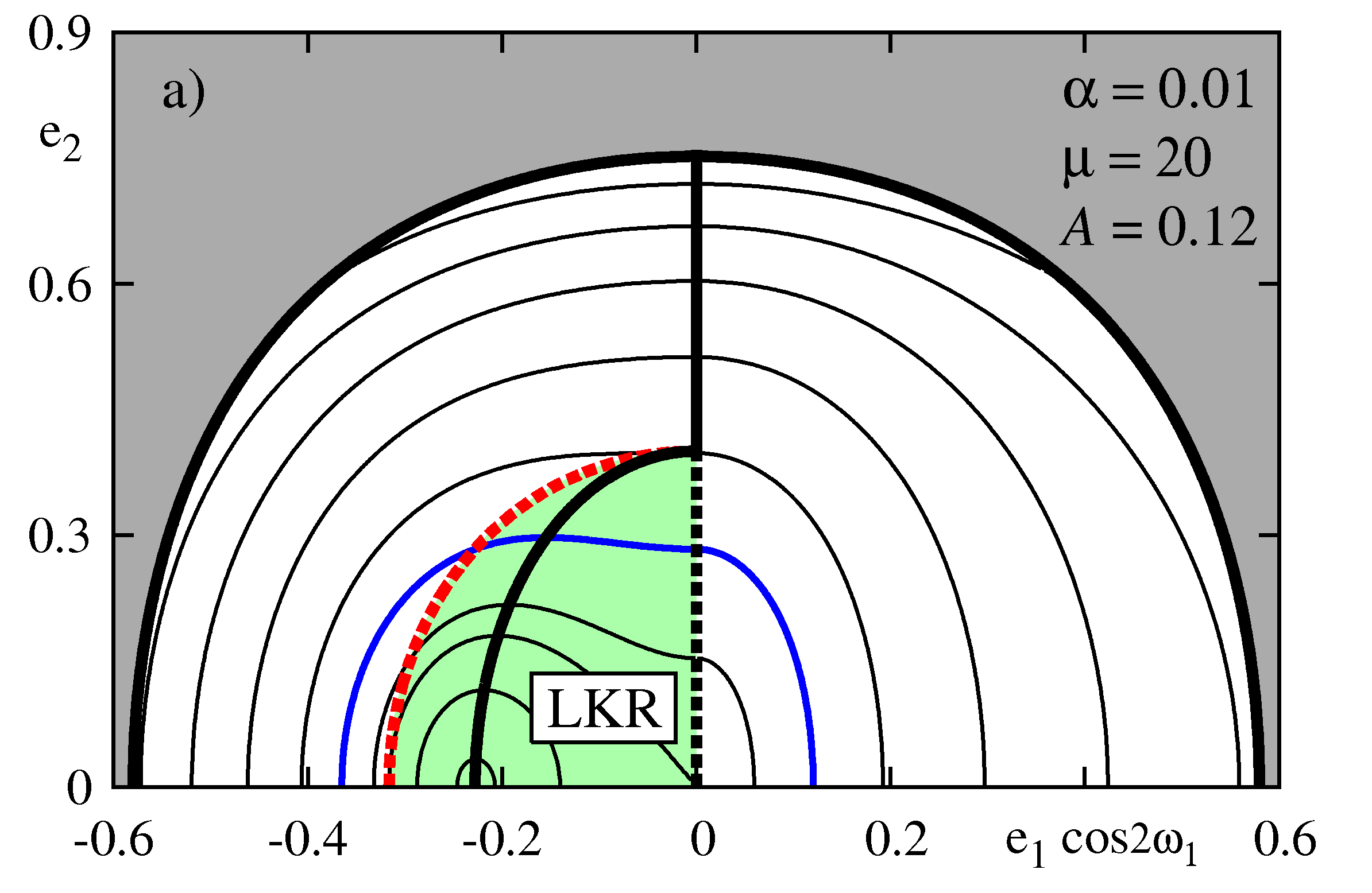
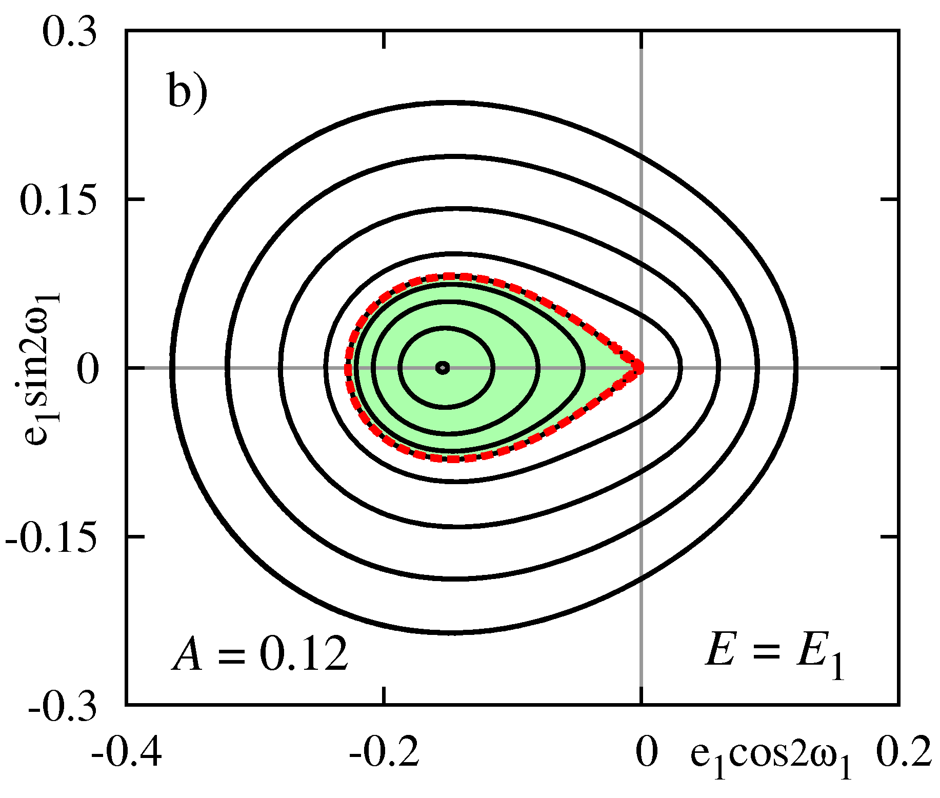
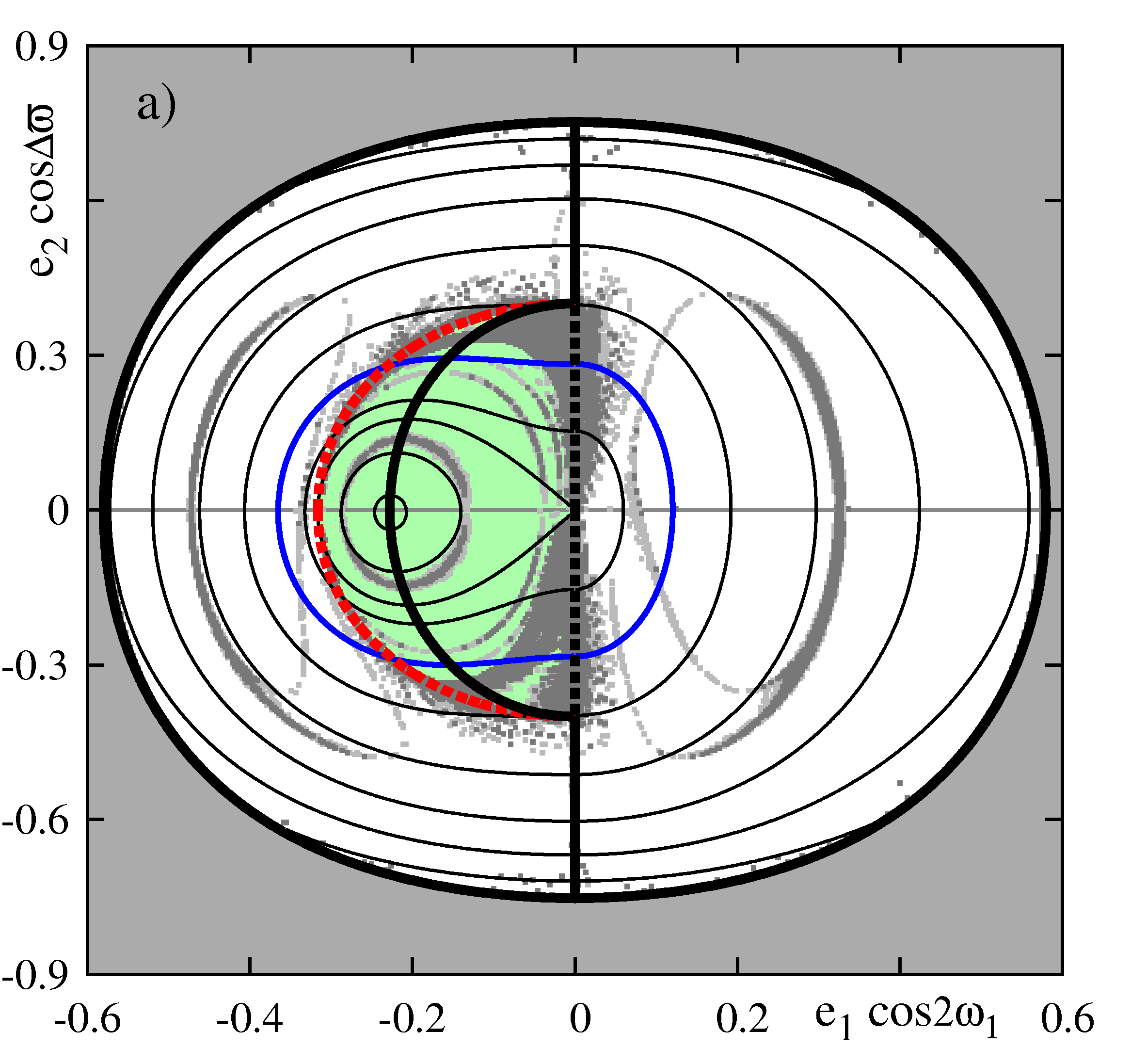
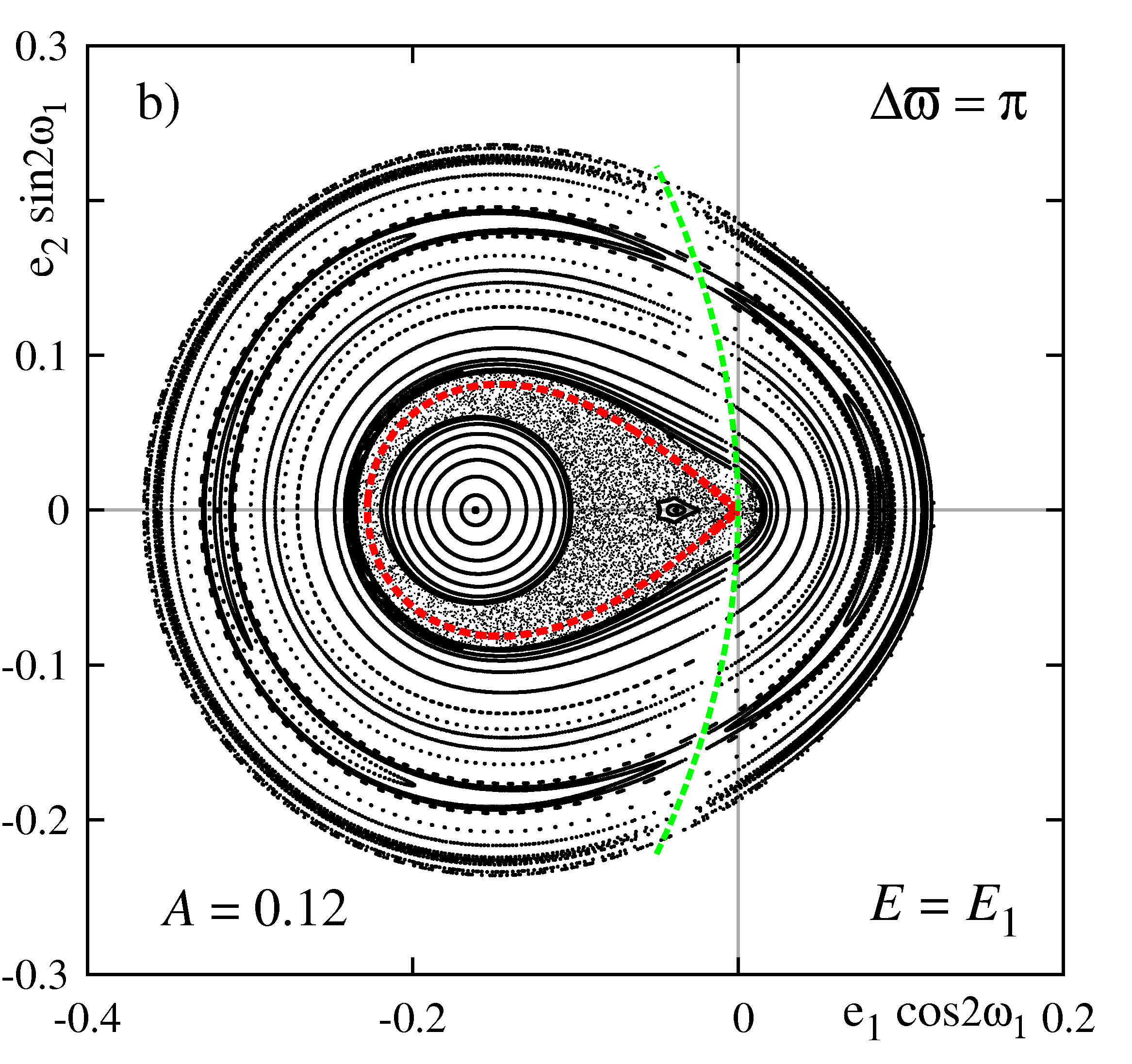
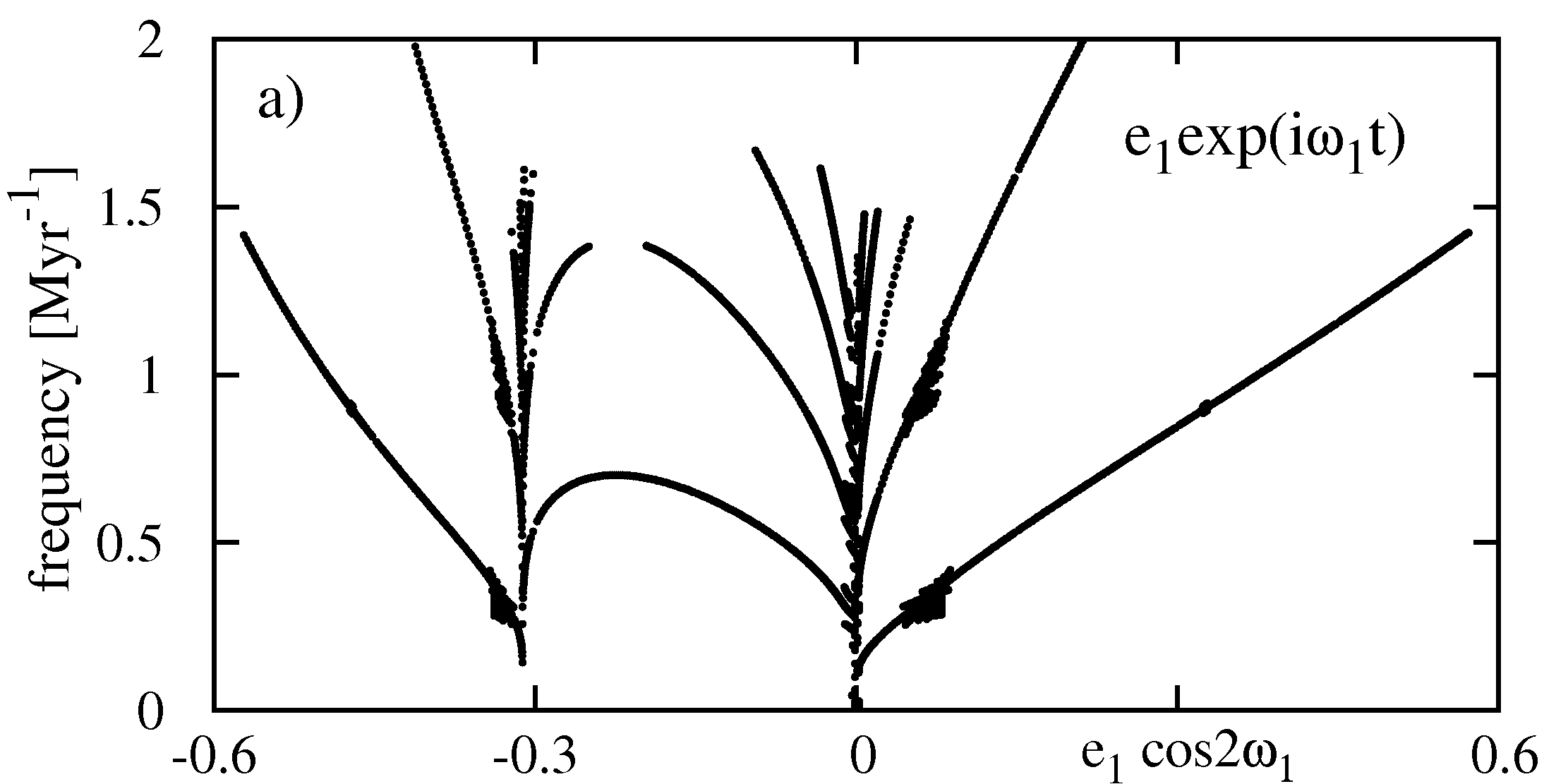
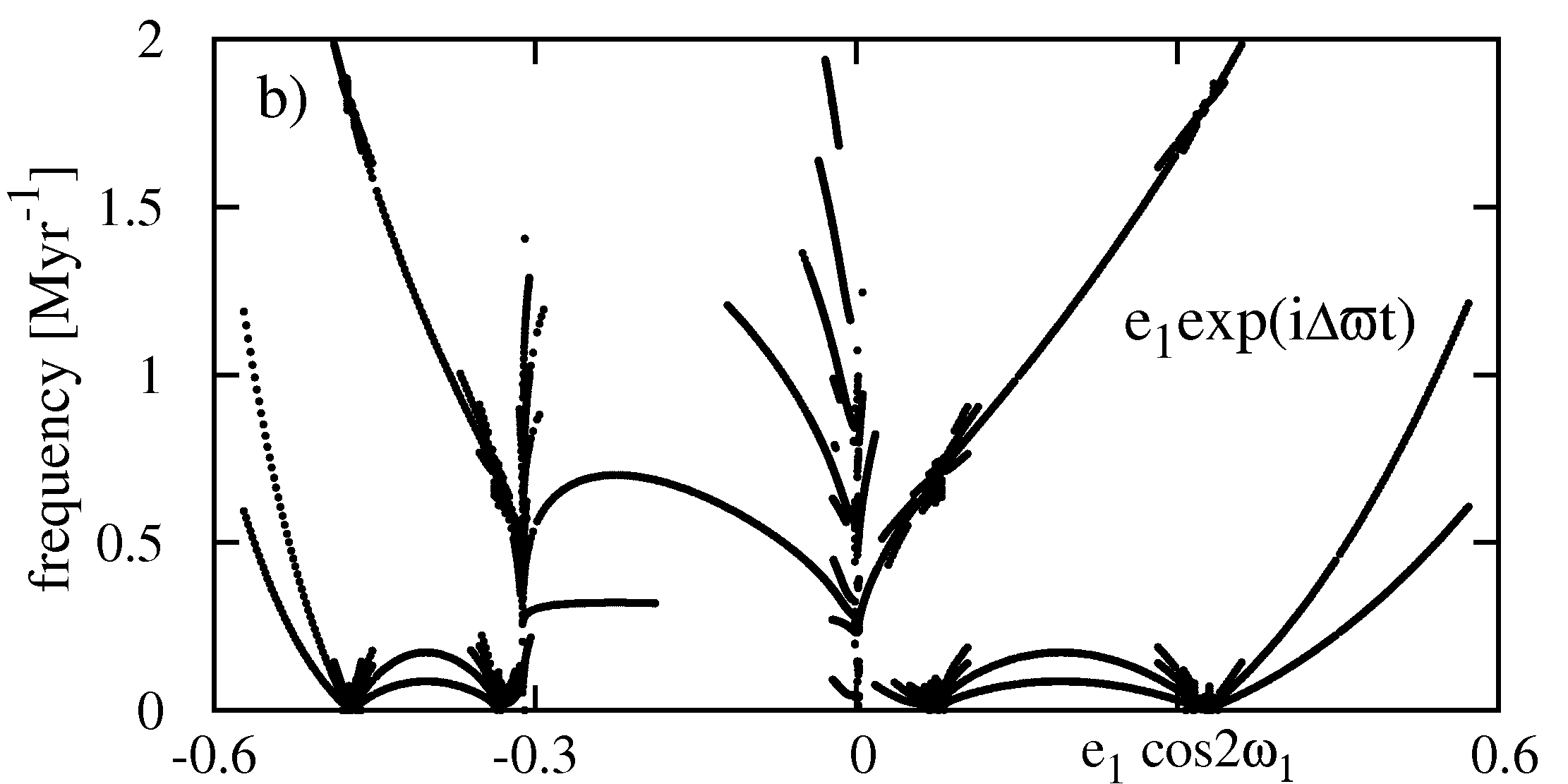
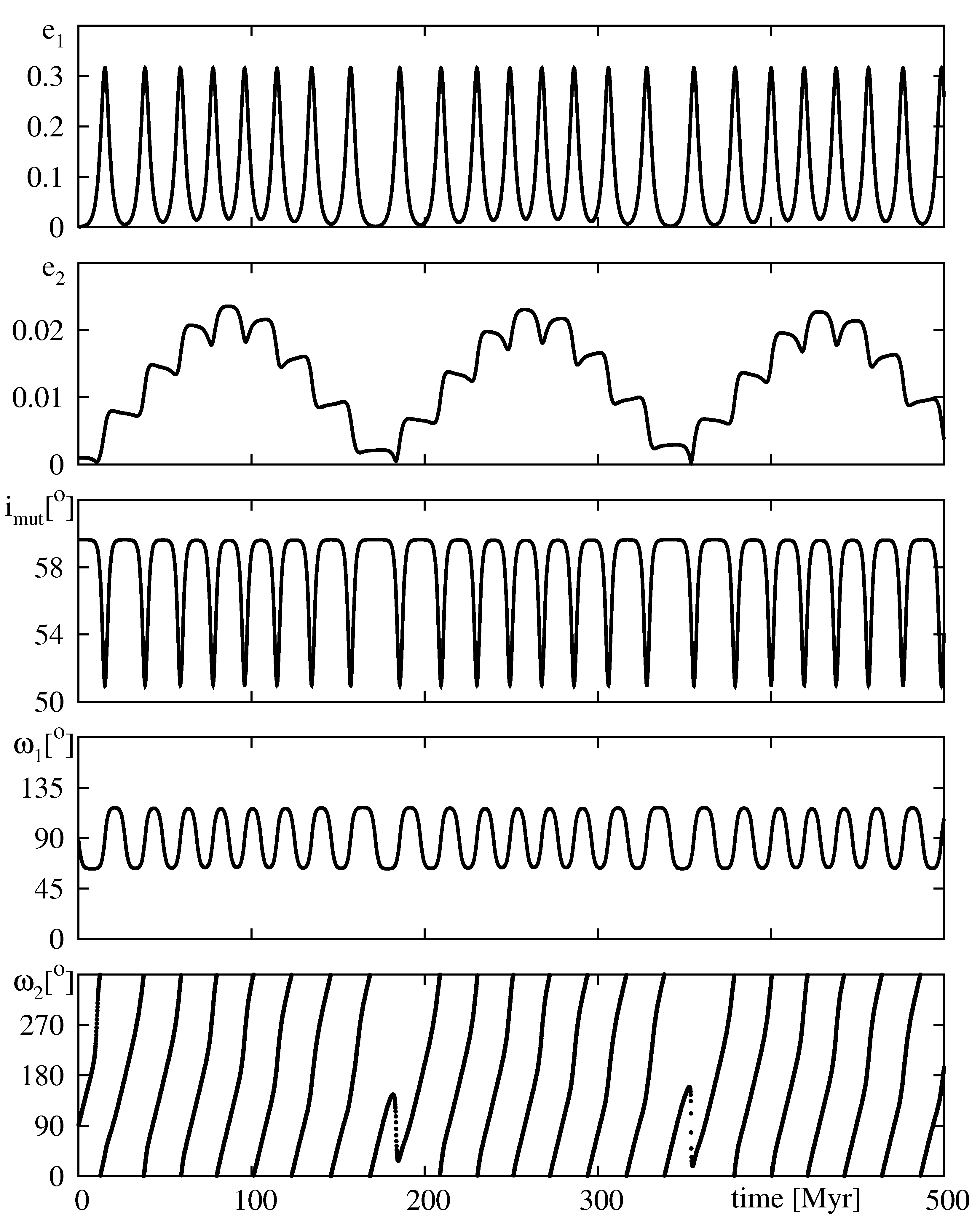
Figure 10 shows the temporal evolution of the mean orbits with initial conditions close to the origin in Fig. 4 (see its caption for the details). The eccentricity of the inner orbit is significantly perturbed while the outer orbit is almost unchanged. The mutual inclination evolves in anti-phase with $e_{1}$, and $\omega_{1}$ librates around $\pi/2$. These are typical features of the Lidov-Kozai resonance, still we recall that in this instance, the smaller outer body forces the LK cycles on the orbits of much more (20 times) massive than the inner component of the binary.

5 Equilibria in the classic octupole model

The dynamical maps and their analysis show that the equilibria constrain the secular dynamics of the perturbed model. In terms of the Newtonian, point-mass formulation, the stationary solutions depend on parameters $\alpha$ and $\mu$. Limiting our survey to $i_{{\mbox{\scriptsize mut}}}<\pi/2$ (direct orbits), we perform a parametric survey of the equilibria in terms of the octupole expansion, in such a manner that a comparison with the results derived for the more general, relativistic model will be possible. Here, we consider a more extended range of mass ratio $\mu$, covering a transition from the planetary regime (small $\mu$) to the circumbinary case (large $\mu$ ) than in (Migaszewski & Goździewski, 2009a). Yet the assumption of small $\alpha$ makes it possible to use the analytic formulation of the secular Hamiltonian, which is very precise in terms of the octupole-level approximation, instead of the numerical approach in (Migaszewski & Goździewski, 2009a).

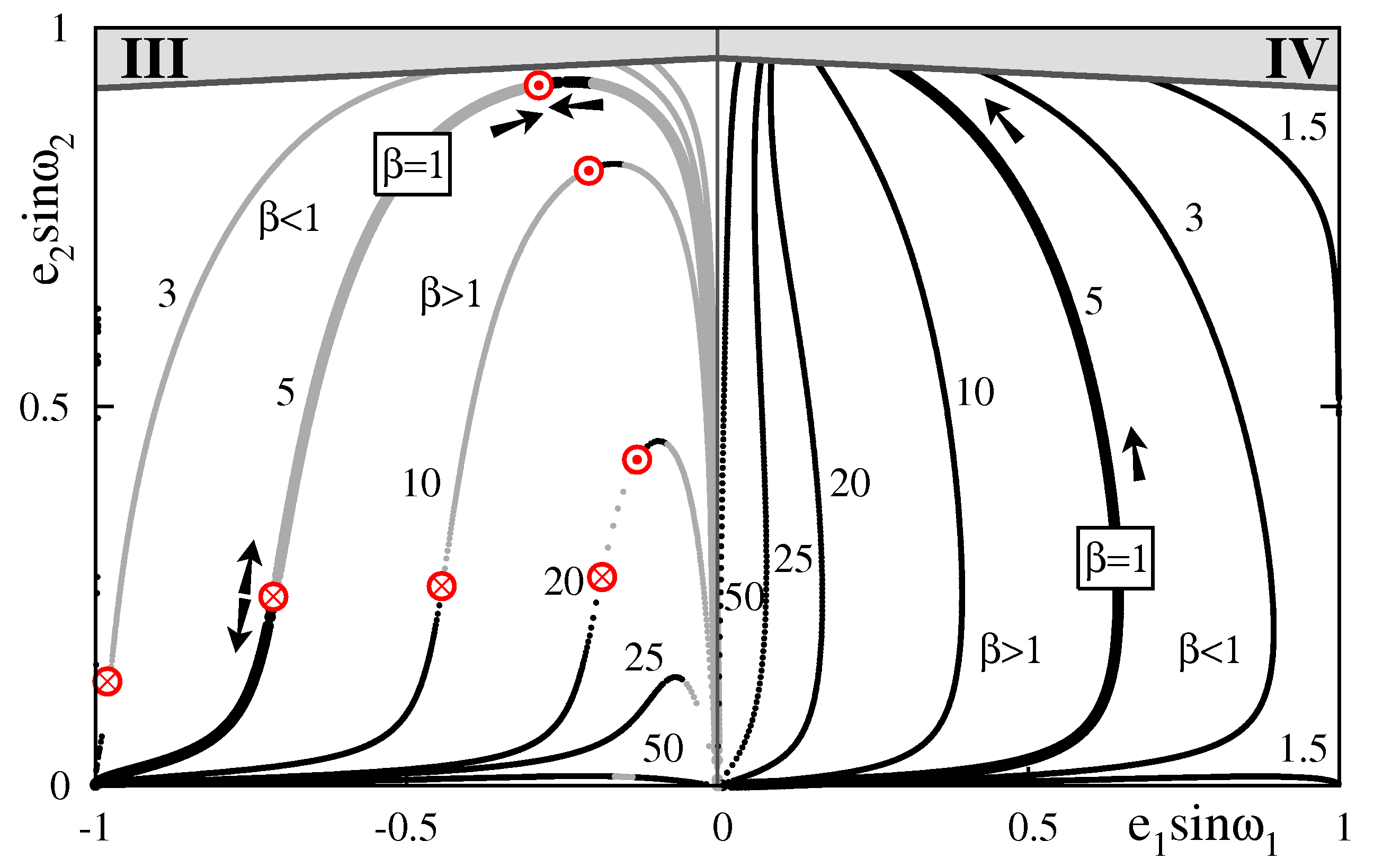
The parameter dependence of the equilibria is illustrated in Fig. 11 that shows the ${\cal P}_{S}$-plane (note that due to the symmetry, only the upper half-plane is illustrated, see also Fig. 3). We set $\alpha=0.04$, $\mu$ $\in[1.5,3,5,10,20,25,50]$, and then positions of the equilibria may be traced along increasing $\mathcal{A}$, which might be understood as the natural curve parameter.

In fact, instead of $\mu$, we choose a new parameter $\beta$ (see Krasinskii, 1974; Migaszewski & Goździewski, 2010)

$$\beta(\mu,\alpha)\equiv L_{1}/L_{2}\sim\mu\sqrt{\alpha},$$

that better reflects the dependence of the dynamics on both $\mu$ and $\alpha$ than on one of these parameters itself (we did a few numerical tests for different $\alpha$ which confirm this scaling very well). Actions $L_{i}$ reflect the angular momentum partition between both components. If $\beta\sim 1$, $(\mu\sim 5)$, both secondaries are dynamically equivalent, if $\beta>1$ ($\mu>5$) then the inner body “dominates” dynamically in the system, and if $\beta<1$ then the hierarchy is reversed. To illustrate the stability of the equilibria, the curves are marked with black dots are for Lyapunov stable solutions, and grey dots mean unstable solutions. The curves are labeled with both $\mu$ and $\beta$ parameters.

In the right-hand half-plane (quarter IV, $\omega_{1}=\omega_{2}=\pi/2$), for $i_{{\mbox{\scriptsize mut}}}<\pi/2$, only one solution appears that is the LK resonance. For small $\mu$, it evolves with increasing $\mathcal{A}$ along the axis of $e_{2}\sim 0$ between $e_{1}=0$ (when the first LK bifurcation appears, see Fig. 2b) and $e_{1}\sim 1$. After the second bifurcation of the LKR (Fig.  2e), two solutions emerge. One of them is the LKR for $i_{{\mbox{\scriptsize mut}}}>\pi/2$ (see Migaszewski & Goździewski, 2009a, this solution is not discussed here). The second new solution moves along the axis $e_{1}\sim 1$ up to large $e_{2}$.

For $\mu\geq 2$, the LKR does not reach $e_{1}=1$ but it “turns back”, with decreasing $e_{1}$ and increasing $e_{2}$. For larger mass ratio, the maximal $e_{1}$ is smaller. The families of LKR for $\mu=1.5,3$ correspond to systems with $\beta<1$, hence the dynamical hierarchy is reversed, and the eccentricity of the inner, more massive body is forced by the outer companion. The position of the LKR family moves to the region of smaller $e_{1}$, and for large enough $\mu$, this solution is confined to $e_{1}\sim 0$-axis and tends to large $e_{2}$. The direction of parametric evolution of this equilibrium, corresponding to increasing $\mathcal{A}$, is marked with an arrow. We see that for all $\mu$ this direction is the same.

The view of the left-hand half-plane is more complex. As we shown in (Migaszewski & Goździewski, 2009a), the first solution appearing in quarter III of the ${\cal P}_{S}$-plane is unstable equilibrium IIIa emerging due to the second bifurcation of the origin $(e_{1}=e_{2}=0)$ (marked with $I_{1}^{-}$ in our paper). Then, with increasing $\mathcal{A}$ , this solution moves along $e_{1}\sim 0$ towards large $e_{2}$. For some value of $\mathcal{A}$ (e.g., $\sim 0.195$ for $\alpha=0.01$, $\mu=20$; see Fig. 3) solutions IIIb and IVb+ appear in the same point of the phase space (this is illustrated with crossed circle in the left-hand half-plane of Fig. 3). Solution IVb+ then moves along $e_{1}\rightarrow 1$ and $e_{2}\rightarrow 0$. Simultaneously, solution IIIb evolves towards a point marked with dotted circle. Solution IIIa also moves to that point and for some critical $\mathcal{A}$ both solutions merge and vanish. Figure 11 reveals that the parametric paths of equilibria depend on parameter $\mu$ ($\alpha=0.04$ was fixed in this test). The path of the LKR becomes closer to $e_{1}\sim 0$-axis for larger mass ratio. Also families of stationary solutions that are present in quarter III, become closer to the origin. The range of eccentricities corresponding to these equilibria is very small for $\mu\geq 25$. We may also notice that the bifurcation points (crossed and dotted circles, respectively) tend to each other with increasing mass ratio, which is consistent with the transition between the planetary and the circumbinary regime. For $\mu\geq 25$, these two points are merged. In this particular case, the structure of equilibria in quarter III of the ${\cal P}_{S}$-plane is more simple than in the general case because only one solution persists, a stable equilibrium corresponding to nearly circular outer orbit.

Figure 11: Families of stationary solutions in the ${\cal P}_{S}$-plane. The semi-major axes ratio $\alpha=0.04$, $\mu=\{1.5,3,5,10,20,25,50\}$ (each curve is labeled accordingly with the value of $\mu$). Dark dots are for stable equilibria, grey dots are for unstable equilibria. Crossed and dotted circles mark the positions on the equilibria curves where solutions bifurcate (see the text for details). Small arrows show the directions of the evolution of particular equilibrium with increasing $\mathcal{A}$. Parameter $\beta\equiv L_{1}/L_{2}$ (see the text). Stationary curves corresponding to $\beta=1$ are drown with thicker lines. Stationary solutions were calculated for the octupole classic model. See also Fig. 3.

For different $\alpha<0.1$, the general, global view of the families of equilibria is very similar to the results presented in Fig. 11. In fact, as we noticed previously, the parametric evolution of the equilibria is reflected by parameter $\beta(\mu,\alpha)$, and basically does not depend on the individual values of $\alpha$ and $\mu$.

6 The PN correction to the secular model

The results presented in the previous section illustrate the already well known feature of the classic model (see, e.g., Michtchenko & Malhotra, 2004; Michtchenko et al., 2006). In the approximation of small masses, the secular dynamics of the Newtonian 2-planet, hierarchical model depend on the semi-major axes ratio and planetary mass ratio, and not on individual system parameters, $(a_{1},a_{2},m_{1},m_{2})$. In our works (Migaszewski & Goździewski, 2009b, 2010), we shown that this feature is not preserved in the more general model, including relativistic, rotational and tidal corrections to the Newtonian point-mass interactions. In these settings, the secular dynamics depend on the individual semi-major axes, as well as individual planetary masses. Because the overall structure of the phase space is characterized by the equilibria, we now attempt to show that deviations between these equilibria in the classic and relativistic models become more important when the system dimension scales down ($a_{1},a_{2}$ decrease when $\alpha$ is const), and masses $m_{1},m_{2}$ are smaller, when their ratio $\mu$ is kept constant.

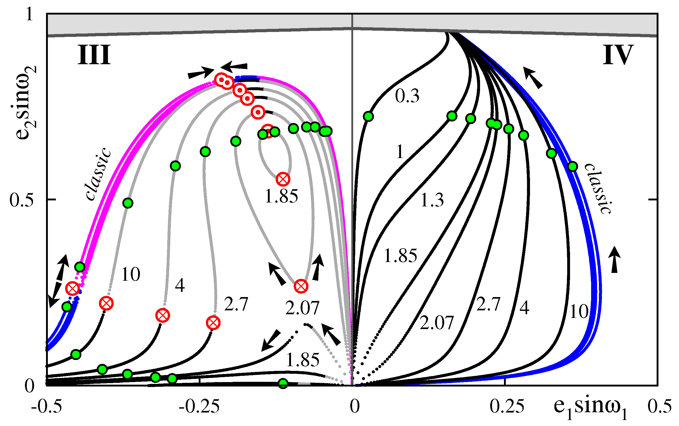
The differences between the two coplanar models manifest itself through the shapes and localization of stationary solutions and depend on the individual masses and semi-major axes (Migaszewski & Goździewski, 2009b). Now we can observe the same feature in the spatial planetary system, corrected for the relativistic perturbation. Figure 12 presents families of equilibria in the same manner as Fig. 11 (due to the symmetry, only the $y$-positive half-plane of ${\cal P}_{S}$-plane is presented). Families of stationary solutions in the classic model are drawn with blue and violet curves for stable and unstable solutions, respectively. Solutions in the relativistic model are plotted with black (stable equilibria) and grey (unstable equilibria) curves. In this experiment, we varied the individual masses of the secondary bodies, still keeping their ratio $\mu=10$ as a constant. The masses are changed between $(m_{1}=100~{}\mbox{m}_{{\mbox{\scriptsize J}}},m_{2}=10~{}\mbox{m}_{{\mbox{\scriptsize J}}})$ to $(m_{1}=3~{}\mbox{m}_{{\mbox{\scriptsize J}}},m_{2}=0.3~{}\mbox{m}_{{\mbox{\scriptsize J}}})$, and the primary mass is $m_{0}=1~{}\mbox{m}_{\odot}$.

The results illustrated in Fig. 12 confirm that even for large secondary masses, the parametric curves of stationary solutions in the realm of the classic model depends weakly on the individual masses. Yet similarly to the co-planar case, curves of equilibria calculated with the relativistic corrections differ significantly from the results obtained for the classic model. The deviations between both models are more significant for smaller masses of the secondary bodies. For instance, the family IVa moves to the range of much smaller $e_{1}$. Solutions of this type exist even for very small $m_{1}$ and $m_{2}$, which is just not possible in the Newtonian model (Migaszewski & Goździewski, 2009a). When the mutual perturbations between secondaries are small enough, the critical inclination in the relativistic model, that leads to the LK bifurcation, becomes larger than $\pi/2$ . Thus $i_{{\mbox{\scriptsize crit}}}$ increases with decreasing masses.

In quadrant III of the ${\cal P}_{S}$-plane ($\omega_{2}=-\omega_{1}=\pm\pi/2$), the structure of equilibria is even more complex. For some critical values of masses ($m_{2}\sim 2.07~{}\mbox{m}_{{\mbox{\scriptsize J}}}$) the parametric paths divide into two parts. The top part, characterized by larger $e_{2}$, comprises of two unstable equilibria emerging from one bifurcation point, which then meet in another bifurcation point. The bottom part of the equilibria curve represents a saddle point, that changes its stability, from unstable IIIa-type solution to the stable solution IVb+. This branch is very similar to equilibria in the classic system with large $\mu$ (or large $\beta>5$) observed already in Fig.  11, however this takes place for quite a different value of $\beta=2$.

Figure 12: Families of stationary solutions presented in the ${\cal P}_{S}$-plane, calculated for $\alpha=0.04,\mu=10,a_{1}=0.2~{}\mbox{au},a_{2}=5.0~{}\mbox{au},m_{0}=1~{}\mbox{m}_{\odot}$ and varied $m_{2}=10,4,2.7,2.07,1.85,1.3,1.0,0.3~{}\mbox{m}_{{\mbox{\scriptsize J}}}$. Equilibria in the classic model are compared with the equilibria in the relativistic model. The mass of the outer body $m_{2}$ labels each particular curve. Black dots are for stable equilibria, grey dots are for unstable equilibria of the relativistic model. Equilibria of the classic model are plotted with blue and violet dots for stable and unstable solutions, respectively. Positions of equilibria were calculated with the help of the octupole theory.

The stationary solutions are determined by the shape of the secular Hamiltonian. Its levels are plotted in the ${\cal P}_{S}$-plane, Fig. 13. Each panel in this figure is calculated for the same parameters $\mu$, $\alpha$, $\mathcal{A}$ (but in this case, particular values of masses and semi-major axes are varied). Let us recall, that Fig. 13a shows the phase space calculated in classic model, while subsequent panels 13b,c,d are for relativistic model, and different masses and semi-major axes, labeled in subsequent panels.

If the masses are large (Fig. 13b), we can see four elliptic points separated by four saddles (let us recall that the ${\cal P}_{S}$-plane is redundant, and the energy levels are reflected with respect to the origin, thus in fact we have only two unique elliptic points and only two saddles). The elliptic points may be identified with solutions IVa ($\omega_{1}=\omega_{2}=\pm\pi/2$) and IIIb ($\omega_{1}=-\omega_{2}=\pm\pi/2$). The saddles correspond to solutions IIIa ($e_{1}\sim 0$) and IVb+ ($e_{2}\sim 0$). When the masses decrease (still, $\mu$ is kept constant), the structure surrounding solution IIIb becomes smaller and moves towards solution IIIa. Simultaneously, the saddle point IVb+ tends to the origin. For the masses small enough, (Fig. 12), solutions IIIa and IIIb merge and vanish, while IVb+ “falls” into the origin.

           

Figure 13: Energy levels presented in the ${\cal P}_{S}$-plane, and calculated for the following parameters $\alpha=0.04,\mu=10,\mathcal{A}=0.215,i_{0}=84^{\circ}$, $a_{1}=0.2~{}\mbox{au},a_{2}=5.0~{}\mbox{au},m_{0}=1~{}m_{\odot}$. A sequence of panels demonstrates the view of the phase space when masses of the secondary bodies decrease (their ratio is constant). From panel b) to panel d) $(m_{1},m_{2})[\mbox{m}_{{\mbox{\scriptsize J}}}]$ are $(100,10),(18.5,1.85),(10,1)$. Shaded areas mark ranges of $i_{{\mbox{\scriptsize mut}}}$ larger than $60^{\circ},75^{\circ}$, (the light– and dark– grey, respectively).

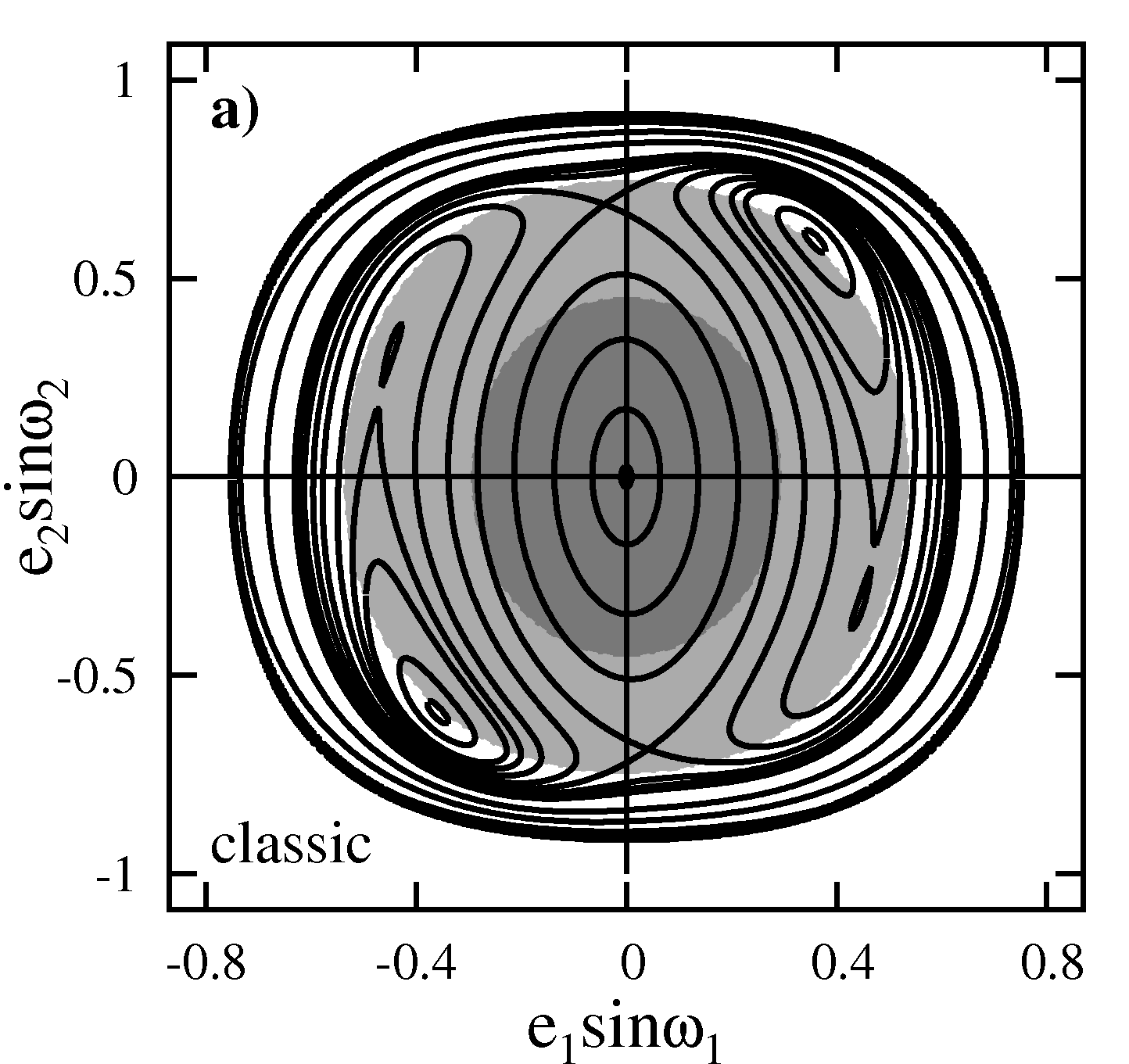
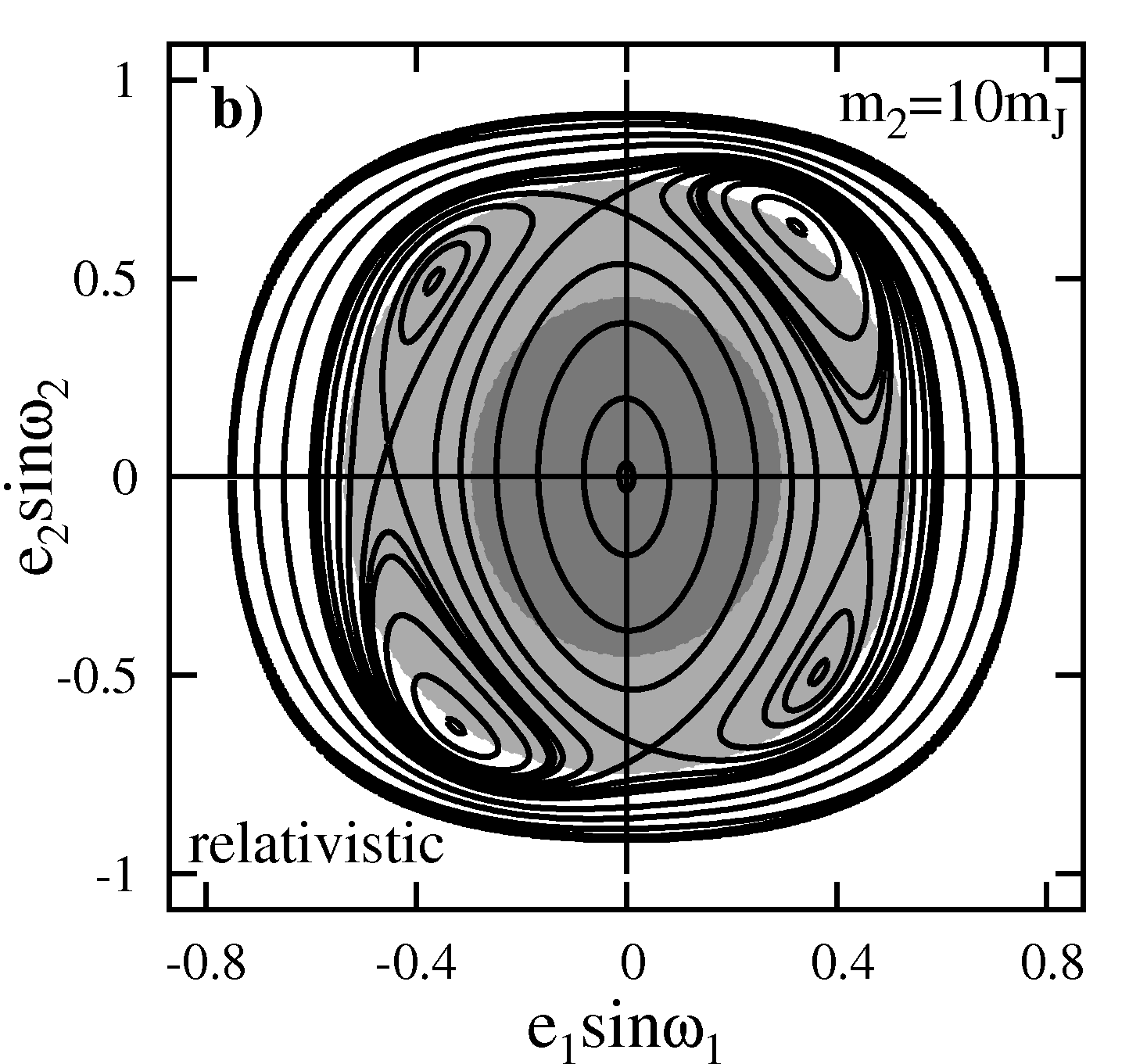
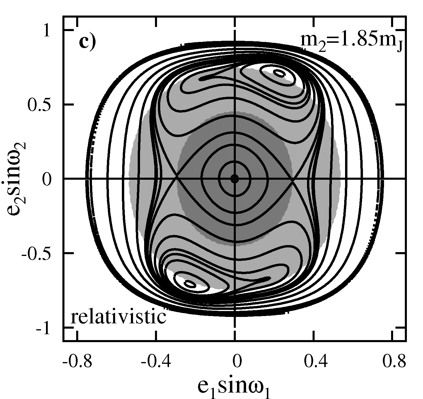
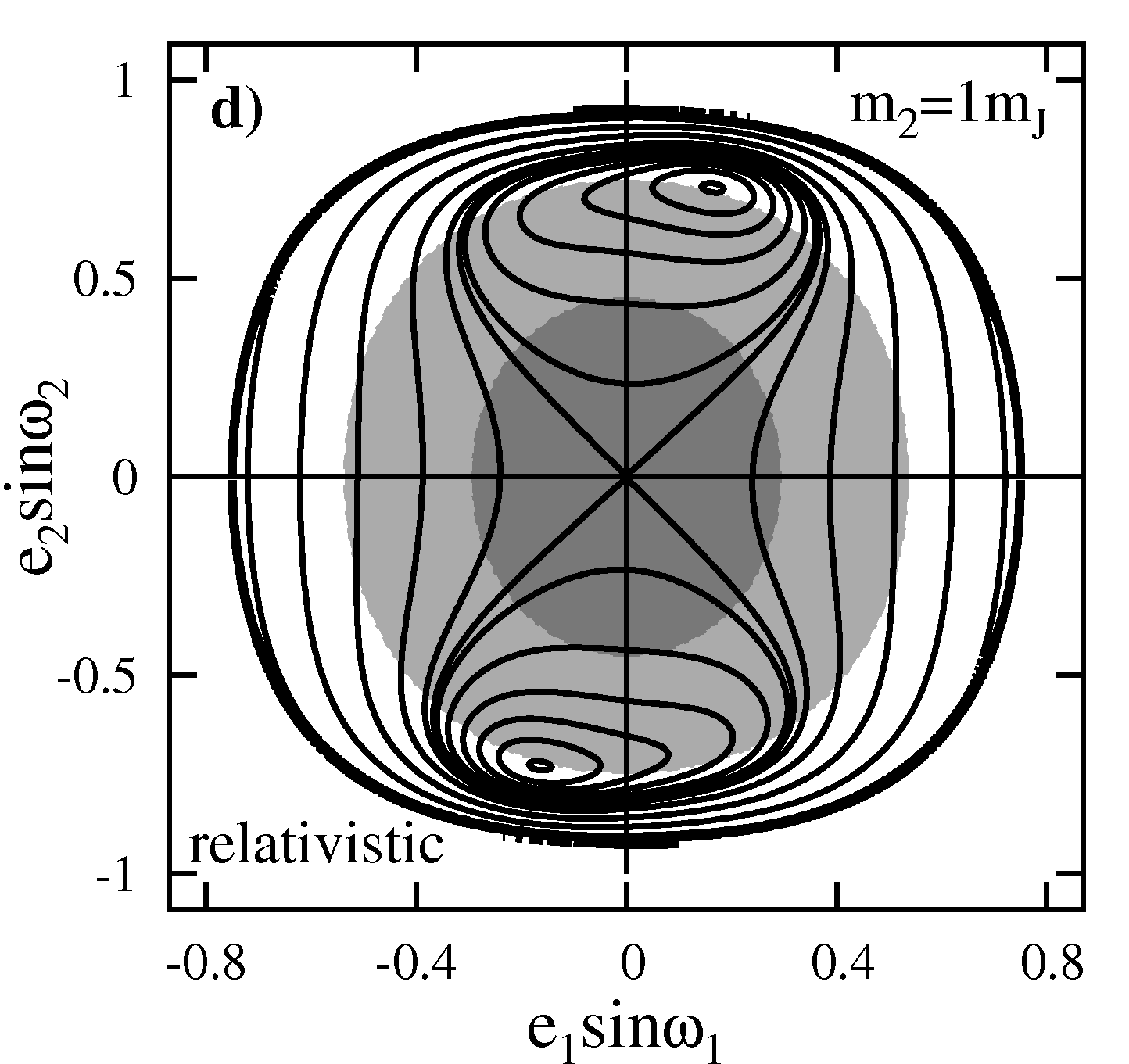
Figures 14–16 shows the dynamical maps for the relativistic model, and are constructed in the same manner as maps in Figs.  4–6. Subsequent figures correspond to masses and $\mathcal{A}$ used to plot the energy levels in Figs. 13a,c,d respectively: Fig.  14 is for classic model, Figs. 15 and  16 are for the relativistic model with $m_{2}=10~{}\mbox{m}_{{\mbox{\scriptsize J}}}$ and $m_{2}=1.85~{}\mbox{m}_{{\mbox{\scriptsize J}}}$, respectively. The mass ratio is $\mu=10$ in both instances. The order of panels and symbol-coding of equilibria, as well as coding libration zones of the angles $\omega_{1}$, $\omega_{2}$, and $\Delta\varpi$ are the same as in Figs. 4–6; in particular, dotted, crossed and empty circles mark the Lyapunov stable, unstable and linearly stable equilibria, respectively. Clearly, the overall view of the phase space is different in all cases. The regions of chaotic motions (yellow areas in the $\sigma$-maps) obtained for the classic and relativistic model are significantly different. Also the dependence on the masses of secondaries in the relativistic models is evident. The structure of chaotic/regular secular evolution is reflected in $\max e_{1,2}$-maps and through librational regions of $\omega_{1}$ and $\omega_{2}$. We note, that in the case of the regular solutions, $\omega_{1}$ librates around $\pm\pi/2$ when $i_{{\mbox{\scriptsize mut}}}>i_{{\mbox{\scriptsize crit}}}$. In some part of this region also $\omega_{2}$ librates around $\pm\pi/2$.

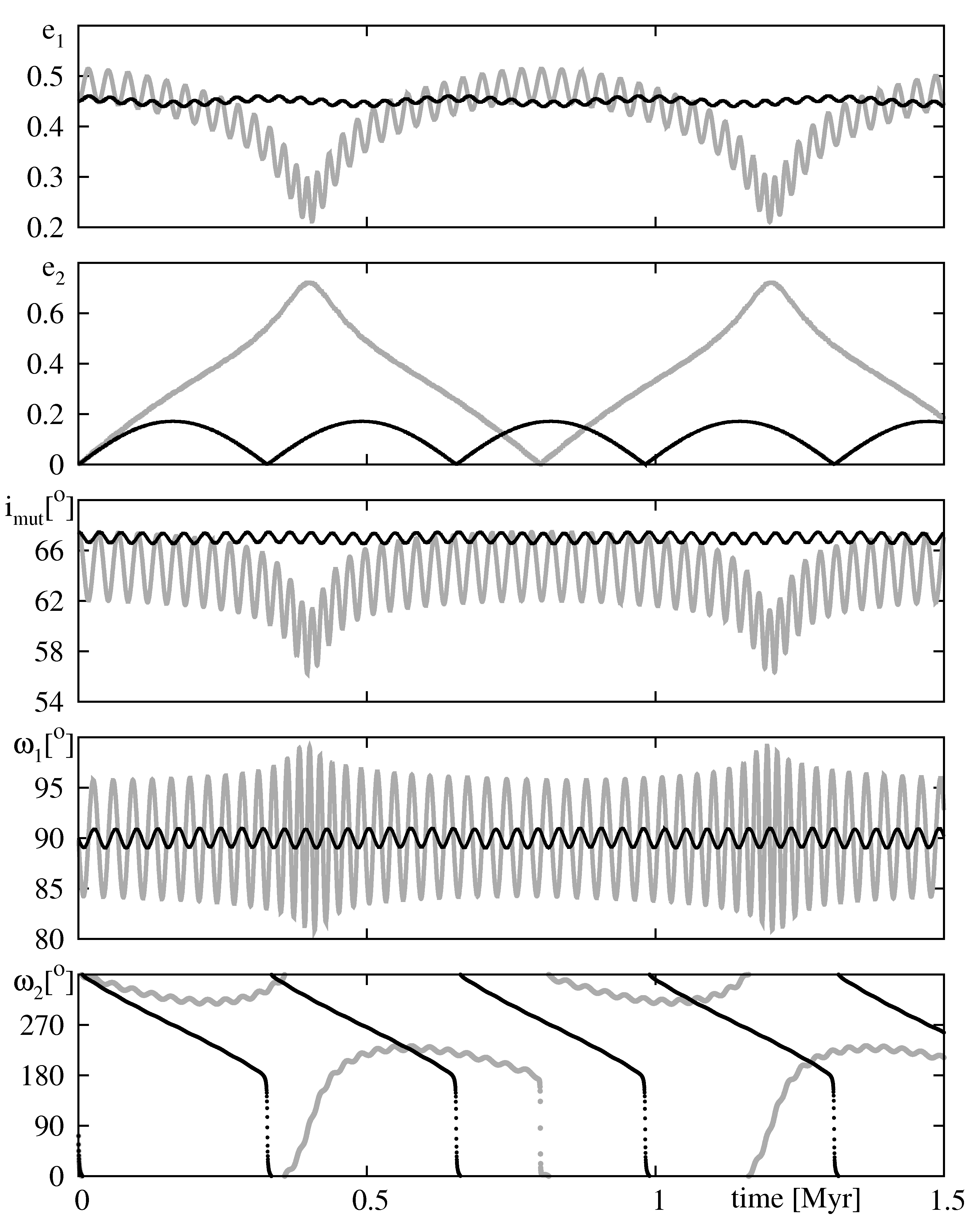
Figure 17 illustrates the temporal evolution for an initial condition written in the caption. The parameters of this model are the same as in Fig. 14. We chose the same initial eccentricities $e_{1}=0.45$ and $e_{2}=0.001$, and integrate the secular equations of motion of classic (grey curves) and relativistic (black curves) models. We note qualitative differences between both configurations. The classic model leads to much larger variations of the elements. Particularly, the outer eccentricity $e_{2}$ is strongly amplified, compared to the variations in the relativistic model. Still, this is not a rule. Inspecting the bottom row of Fig. 16, we can find regions in the ${\cal P}_{S}$-plane, in which, for the same initial condition, $\max e_{2}$ becomes larger in the relativistic model than in the Newtonian model. Also the secularly chaotic configurations appear in quite different zones of the phase space in both models. Moreover, the relativistic corrections may transform the regular evolution in the classic model into the chaotic evolution in the relativistic systems, and vice versa. Remarkably, the configuration illustrated in Fig. 14 has very large masses $m_{1}=100~{}\mbox{m}_{{\mbox{\scriptsize J}}}$ and $m_{2}=10~{}\mbox{m}_{{\mbox{\scriptsize J}}}$.

     

Figure 14: Dynamical maps for the classic, Newtonian model in the ${\cal P}_{S}$-plane. The model parameters are $\alpha=0.04,\mu=10,\mathcal{A}=0.215,i_{0}=84^{\circ}$, $a_{1}=0.2~{}\mbox{au},a_{2}=5.0~{}\mbox{au},m_{0}=1~{}m_{\odot}$, $m_{1}=100~{}\mbox{m}_{{\mbox{\scriptsize J}}}$, $m_{2}=10~{}\mbox{m}_{{\mbox{\scriptsize J}}}$. See the text and caption to Fig. 4 for the details.

     

Figure 15: The dynamical maps for the octupole model with relativistic corrections. Masses of the secondary bodies are $m_{1}=100\,\mbox{m}_{{\mbox{\scriptsize J}}}$, $m_{2}=10\,\mbox{m}_{{\mbox{\scriptsize J}}}$. See the text and caption to Fig. 4 for more details.

     

Figure 16: The dynamical maps for the octupole model with relativistic corrections. Masses of the secondary bodies are $m_{1}=18.5\,\mbox{m}_{{\mbox{\scriptsize J}}}$, $m_{2}=1.85\,\mbox{m}_{{\mbox{\scriptsize J}}}$. See the text and caption to Fig. 4 for more details.

Figure 17: Evolution of the mean orbits in the following system: $m_{0}=1~{}\mbox{m}_{\odot}$, $m_{1}=100~{}\mbox{m}_{{\mbox{\scriptsize J}}}$, $m_{2}=10~{}\mbox{m}_{{\mbox{\scriptsize J}}}$, $a_{1}=0.2~{}\mbox{au}$, $a_{2}=5~{}\mbox{au}$, $e_{1}=0.45$, $e_{2}=0.001$, $\omega_{1}=\pi/2$, $\omega_{2}=\pi/2$, $i_{{\mbox{\scriptsize mut}}}=67^{\circ}.46$, $\mathcal{A}=0.215$. Panels from the top to the bottom illustrate the evolution of $e_{1},e_{2},i_{{\mbox{\scriptsize mut}}},\omega_{1},\omega_{2}$, respectively. The grey curves are for the classic secular model, the black curves are for the model including the relativistic corrections to the potential of the inner binary.

7 Conclusions

In this work, we attempt to show that the global features of the secular dynamics of the 3-D, non-resonant planetary system depend qualitatively on the apparently subtle relativistic corrections to the Newtonian gravity. A lesson, which we learned studying the co-planar case (Migaszewski & Goździewski, 2009b) is that the non-Newtonian point-mass interactions might be very important for the global dynamics, because, in contrary to intuition one may have, the corrections to the Newtonian interactions might be not small, as compared to the mutual point-to-point gravity. The numerical analysis of this multi-parameter problem is complex, hence the underlining idea of this paper lies in a construction of possibly precise analytical model. Essentially simple averaging of the perturbing Hamiltonian in (Migaszewski & Goździewski, 2008), makes it possible to derive the analytic secular theory up to the order of $10$ in the semi-major axes ratio $\alpha$. The accuracy of this model may be compared with the results of the numerical averaging of the perturbation (Michtchenko & Malhotra, 2004). Moreover, for a class of hierarchical systems considered in our paper, already the third-order model is precise enough to find and investigate the qualitative features of the system. In this work, we focus on three-body configurations, e.g., a star and two massive planets or a binary stars and one planet. “Fortunately”, the second-order model is integrable, hence the octupole-level approximation might be considered as the first order perturbation to this analytically soluble case. This makes it possible to understand the sources of instabilities appearing in the full (non-averaged) model.

The averaging over mean anomalies reduces the dynamics to a system having two DOF, which then may be investigated with the help of rich geometrical tools, like the Poincaré cross section and the representative planes of initial conditions introduced in Michtchenko et al. (2006). Unfortunately, all additional corrections that increase the DOF number must be neglected here, as for instance the rotational quadrupole moment of the star and/or of the planets. This is the price that must be paid for the possibly global model of the dynamics. In the assumed range of $a_{1}$ and masses, the relativistic “corrections” in fact compare with the Newtonian point-mass mutual interactions, and are much larger than other perturbations, like the tidal and rotational distortions of the bodies. The analysis of the secular frequencies introduced by various corrections justify that the model only takes into account the PN perturbation to the potential of star and the inner secondary.

Having the two DOF model, we investigate the simplest class of solutions that are the equilibria. We focus on the Lidov-Kozai resonance (LKR) in systems characterized by large range of the mass ratio $\mu$. This part extends the results derived for small $\mu$ in (Migaszewski & Goździewski, 2009a). We found that even much smaller outer body (planetary mass $m_{2}$ with respect to sub-stellar values of $m_{1}$) moving in a wide, highly inclined ($i_{{\mbox{\scriptsize mut}}}>\sim 60^{\circ}$) orbit may significantly perturb the inner orbit. In turn, the restricted model of the circumbinary planet, when we assume that the planet does not influence the binary, is not generally valid, even if the inner mass $m_{1}$ is $100$ times larger than the outer body $m_{2}$.

We also studied the parametric structure of families of particular equilibria classified as IVa, IIIa, IIIb, IVb+ in (Migaszewski & Goździewski, 2009a) for small $\alpha$. Thanks to this assumption, the analytic model makes it possible to investigate the transition between the planetary regime (small $\mu$) and the circumbinary regime ($\mu\sim 50,100$). This study shows that solutions in the planetary problem may disappear for large mass ratio.

A particularly interesting feature of the ocupole model is the appearance of the secular chaos. We found that if $i_{{\mbox{\scriptsize mut}}}$ exceeds the critical inclination $i_{{\mbox{\scriptsize crit}}}(\mu,\alpha)$, the long term evolution of the system may be strongly chaotic, leading to large amplification of the eccentricities. In the regular regions of the phase space, the mean angle $\omega_{1}$ librates around $\pm\pi/2$. In some parts of these regions also the second secular angle $\omega_{2}$ librates around $\pm\pi/2$. The initial conditions satisfying $i_{{\mbox{\scriptsize mut}}}>i_{{\mbox{\scriptsize crit}}}$ lead to strong amplification of the inner eccentricity $e_{1}$. Simultaneously, for the same values of the angular momentum of the system, we may observe strong amplification of $e_{2}$ in some region of the phase space, with almost constant relative inclination of the orbits. This behaviour may be attributed to unstable equilibrium IIIb emerging in the secular system. The amplification of $e_{1}$ happens not only for librations of $\omega_{1}$ around $\pm\pi/2$ (in the LK regime), but also and particularly when this angle behaves chaotically, varying in the whole range of $[0,2\pi]$. The dynamical maps reveal that the primarily source of the chaotic motions are the unstable equilibria and unstable periodic orbits in the full system, following the appearance of separatrices in the integrable, quadrupole-level model.

Thanks to the simple analytic model, the influence of relativistic correction $\mathcal{H}_{{\mbox{\scriptsize GR}}}$ on the global secular dynamics of the problem might be clearly demonstrated. A simple proof of this influence is provided by the analysis of the equilibria in the perturbed model. The differences between the Newtonian and relativistic models are larger when the mutual interactions between the secondaries are weaker, e.g., when companion masses are smaller. Yet the dynamics are basically very simple up to the limit of the critical inclination, when the first bifurcation of the origin ($e_{1}=e_{2}=0$) occurs, and this feature of the dynamics is preserved in both models.

We stress that although the analysis is done for specific, discrete mass ratios, the results are valid as far the assumptions of the averaging theorem are fulfilled and the corrections besides general relativity are negligible. We demonstrated that similarly to the co-planar problem, the global 3-D dynamics of the classic, Newtonian model essentially depend only on the ratios of semi-major axes and masses of the secondaries. Hence, although we consider mostly the circumbinary configurations, the results may be are easily extrapolated to the “typical” planetary regime, investigated already (Michtchenko et al., 2006). Moreover, when the PN corrections are added to the model, the dynamics are much more complex. Still the global picture of the phase space is determined by the ratio of these corrections and the Newtonian mutual interactions. Hence, if the system scales down, while this ratio is roughly preserved, the structure of the phase space, determined by stationary solutions of the secular system should not essentially change.

Our approach may be generalized for other perturbations, like the rotational and conservative tidal distortion of the bodies in the system. Unfortunately, in the most general case, the dimension of the hierarchical system cannot be generally reduced to two DOF. Moreover, these perturbations lead to even more interesting and intriguing dynamics, which we investigated in the co-planar and spatial case (e.g., Fabrycky & Tremaine, 2007; Mardling, 2007; Ragozzine & Wolf, 2009; Migaszewski & Goździewski, 2009b). We work on a global approach, suitable for the 3D systems, aiming to publish these results in future papers.

References

- Adams & Laughlin (2006) Adams F. C., Laughlin G., 2006, International Journal of Modern Physics D, 15, 2133
- Arnold et al. (1993) Arnold V. I., Kozlov V. V., Neishtadt A. I., 1993, Dynamical systems III. Mathematical aspects of classical and celestial mechanics. Encyclopaedia of mathematical sciences, Springer Verlag
- Batygin et al. (2009) Batygin K., Bodenheimer P., Laughlin G., 2009, ApJL, 704, L49
- Brouwer & Clemence (1961) Brouwer D., Clemence G. M., 1961, Methods of celestial mechanics. New York: Academic Press, 1961
- Brumberg (2007) Brumberg V., 2007, Celestial Mechanics and Dynamical Astronomy, 99, 245
- Eggenberger (2010) Eggenberger A., 2010, in K. Goździewski, A. Niedzielski, & J. Schneider ed., EAS Publications Series Vol. 42. pp 19–37
- Fabrycky & Tremaine (2007) Fabrycky D., Tremaine S., 2007, ApJ, 669, 1298
- Farago & Laskar (2010) Farago F., Laskar J., 2010, MNRAS, 401, 1189
- Ferraz-Mello (2007) Ferraz-Mello S., ed. 2007, Canonical Perturbation Theories - Degenerate Systems and Resonance Vol. 345 of Astrophysics and Space Science Library
- Ferrer & Osácar (1994) Ferrer S., Osácar C., 1994, Celestial Mechanics and Dynamical Astronomy, 60, 187
- Ford et al. (2000) Ford E. B., Kozinsky B., Rasio F. A., 2000, ApJ, 535, 385
- Gronchi & Milani (1998) Gronchi G. F., Milani A., 1998, Celestial Mechanics and Dynamical Astronomy, 71, 109
- Harrington (1968) Harrington R. S., 1968, AJ, 73, 190
- Kozai (1962) Kozai Y., 1962, AJ, 67, 579
- Krasinskii (1972) Krasinskii G. A., 1972, Celestial Mechanics, 6, 60
- Krasinskii (1974) Krasinskii G. A., 1974 Vol. 62 of IAU Symposium. pp 95–116
- Laskar (1990) Laskar J., 1990, Icarus, 88, 266
- Laskar (2000) Laskar J., 2000, Physical Review Letters, 84, 3240
- Lee & Peale (2003) Lee M. H., Peale S. J., 2003, ApJ, 592, 1201
- Libert & Henrard (2007) Libert A.-S., Henrard J., 2007, Icarus, 191, 469
- Lidov (1962) Lidov M. L., 1962, Planetary and Space Science, 9, 719
- Lidov & Ziglin (1976) Lidov M. L., Ziglin S. L., 1976, Celestial Mechanics, 13, 471
- Mardling (2007) Mardling R. A., 2007, MNRAS, 382, 1768
- Mardling (2010) Mardling R. A., 2010, MNRAS, 407, 1048
- Michtchenko et al. (2006) Michtchenko T. A., Ferraz-Mello S., Beaugé C., 2006, Icarus, 181, 555
- Michtchenko & Malhotra (2004) Michtchenko T. A., Malhotra R., 2004, Icarus, 168, 237
- Migaszewski & Goździewski (2008) Migaszewski C., Goździewski K., 2008, MNRAS, 388, 789
- Migaszewski & Goździewski (2009a) Migaszewski C., Goździewski K., 2009a, MNRAS, 395, 1777
- Migaszewski & Goździewski (2009b) Migaszewski C., Goździewski K., 2009b, MNRAS, 392, 2
- Migaszewski & Goździewski (2010) Migaszewski C., Goździewski K., 2010, in K. Gożdziewski, A. Niedzielski, & J. Schneider ed., EAS Publications Series Vol. 42, . pp 385–391
- Murray & Dermott (2000) Murray C. D., Dermott S. F., 2000, Solar System Dynamics. Cambridge Univ. Press
- Rabl & Dvorak (1988) Rabl G., Dvorak R., 1988, A&A, 191, 385
- Ragozzine & Wolf (2009) Ragozzine D., Wolf A. S., 2009, ApJ, 698, 1778
- Richardson & Kelly (1988) Richardson D. L., Kelly T. J., 1988, Celestial Mechanics, 43, 193
- Takeda et al. (2009) Takeda G., Kita R., Rasio F. A., 2009, in IAU Symposium Vol. 253 of IAU Symposium, . pp 181–187
- Tamuz, O., et al., (2008) Tamuz, O., et al., 2008, A&A, 480, L33
- Šidlichovský & Nesvorný (1996) Šidlichovský M., Nesvorný D., 1996, Celestial Mechanics and Dynamical Astronomy, 65, 137