Deriving an X-ray luminosity function of dwarf novae based on parallax measurements

Abstract

We have derived an X-ray luminosity function using parallax-based distance measurements of a set of 12 dwarf novae, consisting of Suzaku, XMM-Newton and ASCA observations. The shape of the X-ray luminosity function obtained is the most accurate to date, and the luminosities of our sample are concentrated between $\sim$ 10³⁰–10³¹ erg s^-1, lower than previous measurements of X-ray luminosity functions of dwarf novae. Based on the integrated X-ray luminosity function, the sample becomes more incomplete below $\sim$ 3 $\times$ 10³⁰ erg s^-1 than it is above this luminosity limit, and the sample is dominated by X-ray bright dwarf novae. The total integrated luminosity within a radius of 200 pc is 1.48 $\times$ 10³² erg s^-1 over the luminosity range of 1 $\times$ 10²⁸ erg s^-1 and the maximum luminosity of the sample (1.50 $\times$ 10³² erg s^-1). The total absolute lower limit for the normalised luminosity per solar mass is 1.81 $\times$ 10²⁶ erg s^-1 M${}_{\odot}^{-1}$ which accounts for $\sim$ 16 per cent of the total X-ray emissivity of CVs as estimated by Sazonov et al. (2006).

1 Introduction

Cataclysmic variables, i.e. CVs consist of an accreting white dwarf primary and a late-type main sequence star, and accrete via Roche lobe overflow. CVs can be divided into several subclasses of which so called dwarf novae (DNe) are the most numerous subclass of CVs in our Galaxy. In these systems, the white dwarf has a weak magnetic field strength (B $\lesssim$ 10⁶ G, van Teeseling, Beuermann, & Verbunt, 1996) compared to magnetic CVs, such as polars, and thus the formation of an accretion disc is possible. From time to time, the disc is seen to brighten by several magnitudes lasting from days to several weeks. This brightening of the disc, i.e. an outburst, is thought to be caused by disc instabilities, which are described in detail in Lasota (2001). In quiescence, DNe are sources of optical emission emanating from the accretion disc and the bright spot where the material from the secondary hits the edge of the disc. Quiescent optical spectra of DNe are characterized by strong Balmer emission lines and weaker He I lines with some heavier elements. Also, DNe are sources of hard X-rays which are thought to originate from an optically thin boundary layer during quiescence. However, during an outburst hard X-rays are quenched as the boundary layer becomes optically thick and thus a source of soft X-rays and EUV emission (Pringle, 1977; Pringle & Savonije, 1979).

At the time of the discovery of the Galactic Ridge X-ray Emission (GRXE) in 1982 (Worrall et al., 1982), discrete point sources were thought to be the origin of the GRXE emission. However, the origin has been debated since, but observational evidence gathered to date since the GRXE discovery supports the view that the GRXE is not due to diffuse origin but due to discrete point sources, such as CVs and other accreting binary systems (see recent studies by e.g. Revnivtsev, Vikhlinin & Sazonov, 2007; Revnivtsev et al., 2008). More supporting evidence was given by the recent Chandra study carried out by Revnivtsev et al. (2009) who resolved over 80 per cent of the GRXE into point sources in the 6–7 keV energy range during an ultra-deep 1 Msec observation.

Based on EXOSAT observations of the X-ray emission in the Galactic Plane, Warwick et al. (1985) concluded that if the GRXE is assumed to be originating from discrete point sources, the bulk of the emission observed must be due to a population of low luminosity X-ray sources (L_x $<$ 10^33.5 erg s^-1), such as CVs. Subsequently, Mukai & Shiokawa (1993) suggested that DNe could significantly contribute to the GRXE based on their study of an EXOSAT Medium Energy (ME) DN sample. According to this study, the space density of DNe is sufficiently high to account for a significant fraction of the GRXE. Later on, Ebisawa et al. (2001) resolved sources down to 3 $\times$ 10^-15 erg cm^-2 s^-1 in their Chandra observation of the Galactic Ridge, equivalent to $L_{x}$ $>$ 2.3 $\times$ 10³¹ erg s^-1 at 8 kpc, concluding that the number of resolved point sources above this level is insufficient for them to be the major contributor to the GRXE. Since these previous works have not completely resolved the contribution of CVs to the GRXE, further studies are needed. As was noted by Mukai & Shiokawa (1993), unbiased and sensitive surveys with accurate distance measurements of CVs are needed. This way, accurate X-ray luminosity functions (XLFs) can be obtained, and the contribution to the GRXE estimated more precisely.

The motivation for our work was mainly given by the inaccuracies in the XLFs of Galactic CV populations, such as those by Baskill, Wheatley, & Osborne (2005) and Sazonov et al. (2006). Baskill et al. derived an XLF using 34 ASCA observations of non-magnetic CVs (including 23 DN observations). Their sample lacked accurate distance measurements as only 10 sources had parallax-based distance measurements. Furthermore, this sample was biased by high X-ray flux sources since ASCA was intended to be a spectroscopic mission and the sources in the studied sample were known to be X-ray bright. Also, the ASCA study was purely archival without any sample selection (e.g. the distance was not limited) as Baskill et al. chose all non-magnetic CV observations in the archive, they did not filter out sources which were in an outburst state, or restrict the study to one type of objects only. The XLF study by Sazonov et al. (2006) focused on building up an XLF in the 2–10 keV range combining the RXTE Slew Survey (XSS) and ROSAT All-Sky Survey (RASS) observations of active binaries, CVs and young main sequence stars in the luminosity range $\sim$ 10^27.5 $<$ $L_{x}$ $<$ 10³⁴ erg s^-1. However, uncertainties in the luminosities in this study were introduced by inadequate accuracies in the distances, for example, many of the intermediate polars (IPs) in their sample had poorly known distances. Only a few sources had parallax measurements from, e.g., the Hipparcos or Tycho catalogues (astrometric uncertainties $\sim$ 1 mas) and ground-based parallax measurements from Thorstensen (2003). In addition, the RASS luminosities had 50 per cent uncertainties in addition to statistical errors after conversion from the 0.1–2.4 keV to the 2–10 keV range.

The primary aim of this paper is to derive the most accurate shape of the XLF to date by using a carefully selected sample of DNe. In order to achieve this, we aim to minimise the biases seen in other published XLFs by using sample selection criteria described in Section 2. One of the criteria worth mentioning here is that we only use parallax-based distance estimates. The source sample used in this study does not represent a complete sample of DNe within 200 pc: the sample is more of a ”fair sample” which was not chosen based on the X-ray properties of the sources, and which represents typical DNe within the solar neighbourhood. We will consider the possible effects of the optical selection, inherent in the parallax sample, on the XLF which we derive in Section 6 (Discussion). The motivation for choosing a group of DNe as the sample is based on observations of the Galactic CV populations and previous CV population models. Various authors, such as Howell, Rappaport & Politano (1997), Pretorius, Knigge & Kolb (2007a) and Gänsicke et al. (2009), have pointed out that binaries which are brighter in X-rays and show frequent outbursts, may not represent the true majority of Galactic CV population. The discovery methods of CVs usually favour brighter systems, and thus fainter CVs with low mass accretion rates are likely to be under-represented. However, population models of CVs predict that the majority of CVs are short-period systems ($P_{orb}$ $<$ 2.5 h) and X-ray faint (e.g. Kolb, 1993; Howell, Rappaport & Politano, 1997). These models are supported by observational evidence, e.g. Patterson (1984) showed that a sample of CVs with a total space density of 6 $\times$ 10^-6 pc^-3 was dominated by low mass accretion rate, and thus short period, systems. Also, the SDSS study by Gänsicke et al. (2009) showed that orbital periods of intrinsically faint Galactic CVs accumulated in the 80–86 min range; they found that 20 out of 30 SDSS CVs in this period range showed characteristics which implied that they are low mass accretion rate WZ Sge type DNe. As has been shown by these studies, less X-ray luminous objects (such as DNe) dominated the studied volumes, and thus we choose to focus on DNe in this paper. It is also worth mentioning the study by Pretorius et al. (2007b) who carried out the ROSAT North Ecliptic Pole (NEP) survey using a purely X-ray flux limited and a complete sample of 442 X-ray sources above a flux limit of $\sim$ 10^-14 erg cm^-2 s^-1 in the 0.5–2.0 keV band (only five systems were CVs). They concluded that if the overall space density of CVs is as high as 2 $\times$ 10^-4 pc^-3, then the dominant CV population must be fainter than 2 $\times$ 10²⁹ erg s^-1.

We have carried out X-ray spectral analysis of our sample of 13 sources and derived an XLF in the 2–10 keV band for 12 of them with reliable distance measurements based on those of by Harrison et al. (2004), Thorstensen (2003) and Thorstensen, Lépine, & Shara (2008). By using sources with accurate distance measurements, we minimise the error on the luminosity. Also, we have carried out timing analysis for 5 sources in the sample which were recently observed by Suzaku. At the time of writing this paper, the Z Cam type star KT Per went into an outburst in January 2009, and thus we also briefly report on the Suzaku observations of KT Per during the outburst in Section 5.5.

2 The selection criteria and the source sample

Since we wanted to obtain accurate luminosities for the sources (and thus an accurate shape for the luminosity function), the first step was to avoid selecting sources randomly from the archive (see e.g. Baskill, Wheatley, & Osborne, 2005) or selecting an X-ray flux limited source sample. The aim was to have a distance-limited sample. Thus, sources were not selected based on their X-ray properties, but we chose only those DNe which have accurately measured distances based on trigonometric parallax measurements within $\sim$ 200 pc. Note that by using all available distance measurement techniques, Patterson (priv. comm.) estimates that currently there are 13 DNe within 100 pc, and $\sim$ 33 DNe within 200 pc from the Sun, of which the latter count is clearly incomplete. Above the 200 pc limit, ground-based parallax technique does not give accurate and reliable distance measurements. By using trigonometric parallax-based distance measurements, we are more likely to avoid biases in the distance measurements which are present in the previous, published X-ray luminosity functions. Due to the lack of ground-based parallax measurement programme for the Southern hemisphere, our sample is limited to northern and equatorial objects. However, this selection should not introduce any biases in terms of the optical or X-ray luminosities in our sample.

The distance measurements of the sources chosen for this work are based on astrometric parallaxes obtained by the Hubble Space Telescope (HST) Fine Guidance Sensors (FGSs) (Harrison et al., 2004), and trigonometric parallaxes obtained by the ground-based 2.4 m Hiltner Telescope at the MDM Observatory on Kitt Peak, Arizona (Thorstensen, 2003; Thorstensen, Lépine, & Shara, 2008) and Thorstensen (in prep.). The first accurate astrometric parallaxes of DNe (SS Cyg, SS Aur and U Gem) were measured in 1999 using the FGSs which can deliver high-precision parallaxes with sub-milliarcsecond uncertainties (Harrison et al., 1999). Trigonometric parallaxes derived by ground-based observations have uncertainties around 1 mas (= 10^-3 arcsec) or less (Thorstensen, 2003; Thorstensen, Lépine, & Shara, 2008) which is almost as good as the uncertainty on the FGS parallax measurements.

The second selection criterion was to restrict the sample to sources which had been observed by X-ray imaging telescopes with CCDs in the energy range 0.2–10 keV. Once we had obtained a list of targets with parallax measurements, we then looked for archival data of pointed imaging X-ray observations of these targets in the energy range $\sim$ 0.2–10 keV. If the chosen targets did not have previous X-ray imaging observations, we requested Suzaku X-ray observations. Finally, we wanted to constrain the sample to those sources which were in their quiescent states during the observations in order to avoid biases in the luminosities, and thus AAVSO light curves of the selected sources were inspected to confirm that the sources were in quiescence during the X-ray observations.

The final source sample consists of 9 SU UMa (including 2 WZ Sge systems), 3 U Gem and 1 Z Cam type DNe. The main characteristic which separates these classes of DNe is the outburst behaviour: U Gem type DNe outburst mainly in timescales of every few weeks to every few months whereas SU UMa stars show normal, U Gem type DN outbursts and, in addition, superoutbursts with superhumps (variations in the light curves at a period of a few per cent longer than the orbital period) in timescales of several months to years. The extreme cases, WZ Sge stars, only have superoutbursts with outburst timescales of decades without normal DN outbursts. The defining characteristic for Z Cam stars is standstills, i.e., it is possible that after an outburst, they do not return to the minimum magnitude (unlike U Gem stars), but remain between the minimum and maximum magnitudes for 10–40 days.

Table 1: The source sample used to derive the X-ray luminosity function (excluding *) with their inclinations, orbital periods, white dwarf masses, distances and DN types. The types given in the last column are U Gem (UG), SU UMa (SU), WZ Sge (WZ) and Z Cam (ZC). The references are: a) Thorstensen (2003), b) Thorstensen, Lépine, & Shara (2008), c) Harrison et al. (2004), d) Mason et al. (2001), e) Urban & Sion (2006), f) Friend, Connon-Smith & Jones (1990), g) Ritter & Kolb (2003), h) Horne, Wood & Stiening (1991), i) Preliminary distance estimate from Thorstensen (in prep.), and j) Templeton et al. (2006).

Source	Inclination	Porb	MWD	Distance	Type
	deg	h	M⊙	pc
SS Cyg	40 $\pm$ 8 c	6.603 c	1.19 f	165${}^{+13}_{-11}$ c	UG
V893 Sco	71 $\pm$ 5 a	1.82 a	0.89 d	155${}^{+58}_{-34}$ a	SU
SW UMa	45 $\pm$ 18 g	1.36 b	0.80 e	164${}^{+22}_{-19}$ b	SU
VY Aqr	63 $\pm$ 13 a	1.51 a	0.8/0.55 e	97${}^{+15}_{-12}$ a	SU
SS Aur	40 $\pm$ 7 c	4.39 a	1.03 e	167${}^{+10}_{-9}$ c	UG
BZ UMa	60–75 e	1.63 b	0.55 e	228${}^{+63}_{-43}$ b	SU
U Gem	69 $\pm$ 2 c	4.246 c	1.03 e	100 $\pm$ 4 c	UG
T Leo	47 $\pm$ 19 a	1.42 a	0.35 e	101${}^{+13}_{-11}$ a	SU
WZ Sge	76 $\pm$ 6 c	1.36 a	0.90 e	43.5 $\pm$ 0.3 c	SU/WZ
HT Cas	81 $\pm$ 1 h	1.77 b	0.8 e	131${}^{+22}_{-17}$ b	SU
GW Lib	11 $\pm$ 10 a	1.28 a	0.8 e	104${}^{+30}_{-20}$ a	SU/WZ
Z Cam∗	65 $\pm$ 10 a	6.98 a	1.21 e	163${}^{+68}_{-38}$ a	ZC
ASAS J0025	–	1.37 j	–	$\sim$ 175${}^{+120}_{-40}$ i	SU

The sources, which were included in the calculation of the X-ray luminosity function and when testing different correlations discussed later in this paper, were observed with Suzaku (BZ UMa, SW UMa, VY Aqr, SS Cyg, SS Aur, V893 Sco, and ASAS J002511+1217.2), XMM-Newton (U Gem, T Leo, HT Cas and GW Lib) and with ASCA (WZ Sge). Suzaku observations of BZ UMa, SW UMa, VY Aqr, SS Aur, V893 Sco and ASAS J0025 were requested as these observations were not in the archive. Mukai, Zietsman & Still (2009) discuss the Suzaku observations of V893 Sco in more detail. We also included Z Cam in the source sample since it has a parallax measurement, but it appeared to be in a transition state during the observations. Thus, we have only reported the results of the spectral analysis for Z Cam, but excluded it when calculating the X-ray luminosity function, and when testing correlations between different parameters. The system parameters for all the 13 sources are given in Table LABEL:sources.

3 Observations and data reduction

The details of the Suzaku, XMM, and ASCA observations are given in Table LABEL:observations, and the data reduction methods are described in the following sections.

Table 2: The observation dates and the instruments used in the observations for each source. The exposure times for the Suzaku sources have been obtained from the cleaned event lists, and the numbers in brackets for the XMM sources show exposure times after filtering high background flares. The last column corresponds to the optical state of the source during the observations.

Source	ObsID	Instrument	Tstart	Tstop	Texp	State
					ks
SS Cyg	400006010	XIS/Suzaku	2005-11-02	2005-11-02	39	Q
V893 Sco	401041010	XIS/Suzaku	2006-08-26	2006-08-27	18	Q
SW UMa	402044010	XIS/Suzaku	2007-11-06	2007-11-06	17	Q
VY Aqr	402043010	XIS/Suzaku	2007-11-10	2007-11-11	25	Q
SS Aur	402045010	XIS/Suzaku	2008-03-04	2008-03-05	19	Q
BZ UMa	402046010	XIS/Suzaku	2008-03-24	2008-03-25	30	Q
ASAS	403039010	XIS/Suzaku	2009-01-10	2009-01-11	33	Q
J0025
KT Per	403041010	XIS/Suzaku	2009-01-12	2009-01-13	29	OB
U Gem	0110070401	MOS1/XMM	2002-04-13	2002-04-13	23(22.4)	Q
	0110070401	MOS2/XMM	2002-04-13	2002-04-13	23(22.4)	Q
T Leo	0111970701	PN/XMM	2002-06-01	2002-06-01	13(13)	Q
HT Cas	0111310101	PN/XMM	2002-08-20	2002-08-20	50(6.9)	Q
GW Lib	0303180101	PN/XMM	2005-08-25	2005-08-26	22(6.7)	Q
WZ Sge	34006000	GIS,SIS/ASCA	1996-05-15	1996-05-15	85	Q
Z Cam	35011000	GIS,SIS/ASCA	1997-04-12	1997-04-12	41	T

3.1 Suzaku data reduction

Suzaku (Mitsuda et al., 2007), originally Astro-E2, was launched in 2005 and is Japan’s 5th X-ray astronomy mission. In this paper, we will focus on the X-ray Imaging Spectrometer (XIS) data. The XIS consists of four sensors: XIS0,1,2,3 of which three (XIS0,2,3) contain front-illuminated (FI) CCDs, and XIS1 contains a back-illuminated (BI) CCD. The XIS0,2,3 are less sensitive to soft X-rays than XIS1 due to the thin Si and SiO₂ layers on the front side of the XIS0,2,3 CCDs. Since November 9, 2006, the XIS2 unit has not been available for observations. The Suzaku background is low and hardly affected by soft proton flares often seen in XMM observations.

The unfiltered event lists of SS Cyg and V893 Sco were reprocessed with xispi and screened in xselect with xisrepro since the pipeline version for these observations was older than v.2.1.6.15 which does not include correction for the time- and energy-dependent effects in energy scale calibration. For all the other Suzaku observations, the observations had been processed by more recent pipeline versions and thus reprocessing was not necessary. Pile-up was not a problem for our data since the source count rates were safely below the pile-up limit (12 ct s^-1) for point sources observed in the ’Normal’ mode using Full Window. The Suzaku data reduction described below was carried out in a similar manner for all the Suzaku observations. The cleaned event lists were read into xselect in which X-ray spectra were extracted for each source. Light curves were extracted for SW UMa, BZ UMa, SS Aur, ASAS J0025, and VY Aqr for timing analysis studies. To include 99 per cent of the flux and to obtain the most accurate flux calibration, the spectra and light curves were extracted using a source radius of 260” (250 pixels). The backgrounds were taken as an annulus centred on the source excluding the inner 4’ source region. The outer radii of the background annuli were determined according to how close the calibration sources were to the target. The response matrix files (RMFs) and ancillary response files (ARFs) were created and combined within xisresp v.1.10. The XIS0,2,3 source and background spectra and the corresponding response files were summed in addascaspec to create the total XIS0,2,3 source and background spectra, and the total XIS0,2,3 response file. For the light curves, the background areas were scaled to match the source areas, and the scaled background light curves were then subtracted from the source light curves in lcmath.

3.2 XMM data reduction

XMM-Newton (Jansen et al., 2001) is the cornerstone mission of the European Space Agency (ESA). It has been operating since 1999 with three X-ray cameras (EPIC pn, MOS1 and MOS2), the Optical Monitor (OM), and the Reflection Grating Spectrometer (RGS) onboard. The X-ray cameras cover the energy range 0.2–12.0 keV.

The data were obtained from the XMM-Newton Science Archive (XSA) and the XMM-Newton data were reduced and analysed in the standard manner using the XMM-Newton Science Analysis System sas version 8.0.0. Each observation was checked for high background flares in the range 10–12 keV using single pixel events (pattern == 0). The high background flares were cut above 0.35 ct s^-1 for the MOS data and above 0.40 ct s^-1 for the pn data. The source and background extraction regions were taken from circular extraction areas avoiding any contaminating background sources. The radii of the source regions were calculated by using the sas task region in order to derive source extraction radii which include $\sim$ 90 per cent of the source flux for each source. The background extraction region (r_bg = 130 arcsec) was taken from the same chip as the source extraction region, or from an adjacent chip in case of a crowded source chip. When extracting the X-ray spectra, only well-calibrated X-ray events were selected for all the sources, i.e. for the pn spectra single and double pixel events with pattern $\leq$ 4 were chosen, and in order to reject bad pixels and events close to CCD gaps, FLAG == 0 was used. For the MOS, pattern $\leq$ 12 and #XMMEA_EM were applied.

For most of the observations, we analysed the pn observations only. Since the total effective area of the two EPIC MOS cameras is nearly equal to the effective area of the EPIC pn, the MOS spectra would not add any significant information to the pn spectra. The only exception was U Gem pn observation which had been obtained in Small Window mode. Thus, we used the MOS1 and 2 data which had been obtained in Large and Small window modes, respectively, and selected the backgrounds from the surrounding CCDs. To form the total MOS spectrum for U Gem, the U Gem MOS1 and 2 spectra were summed in addascaspec. All the observations were checked in case of pile-up by using the XMM sas task epatplot. Pile-up did not occur in any of the observations, but the source PSFs of HT Cas and T Leo were contaminated by out-of-time (OoT) events, introduced by these two sources. Therefore, the background regions in the HT Cas and T Leo observations were taken from the adjacent chip in order to avoid the OoT events. These OoT events were removed from the source X-ray spectra according to the ’sas threads’, i.e. the source spectra extracted from the OoT event lists were subtracted from the source spectra extracted from the original event list.

3.3 ASCA data reduction

The Advanced Satellite for Cosmology and Astrophysics (ASCA, Tanaka, Inoue & Holt, 1994) was Japan’s fourth cosmic X-ray astronomy mission operating between February 1993 and July 2000 and was the first X-ray observatory which carried CCD cameras. The main science goal of ASCA was the X-ray spectroscopy of astrophysical plasmas. It carried four X-ray telescopes with two types of detectors located inside them: two CCD cameras, i.e. the Solid-state Imaging Spectrometers (SIS0 and SIS1) with spectral resolution of 2 per cent at 5.9 keV at launch, and two scintillation proportional counters, i.e. the Gas Imaging Spectrometers (GIS2 and GIS3).

The ASCA data reduction was performed in the standard manner by mostly using the standard screening values for the GIS and SIS instruments as described in NASA ASCA online manual. For both instruments, intervals outside the South Atlantic Anomaly (SAA) were chosen, also including intervals when the attitude control was stable with the upper limit of the angular distance from the target set to ang_dist $<$ 0.02 degrees. For the SIS instruments, the bright earth angle of br_earth $>$ 10 was applied excluding the data taken below the 10^∘ angle. Times of high background were excluded when the PIXL monitor count rate was 3$\sigma$ above the mean of the observation. Also, the background monitor count rate of rbm_cont $<$ 500 was applied (the standard screening value is rbm_cont $<$ 100). Events which occurred before the first Day-Night transition and at least 32 seconds after the Day-Night transition, and also before the passage of the South Atlantic Anomaly (SAA) and at least 32 s after the SAA, were selected (T_DY_NT ¡ 0 $\parallel$ T_DY_NT ¿ 32 && T_SAA ¡ 0 $\parallel$ T_SAA ¿ 32).

The source extraction regions for the SIS and GIS were centred on the source. For the GIS, a $\sim$ 6 arcmin circular source extraction region was used for both Z Cam and WZ Sge, while the SIS source extraction regions were smaller so that they could be safely fitted within the chip. Thus, the source extraction radii for Z Cam were 4.4 arcmin (SIS0) and $\sim$ 3.5 arcmin (SIS1) and for WZ Sge $\sim$ 4 arcmin (SIS0) and $\sim$ 3 arcmin (SIS1). The background extraction region for the GIS was taken centred on the detector excluding a circular region of $\sim$ 8 arcmin centred on the source. The background extraction radii for GIS2 and GIS3 were 15.7 and 15.5 arcmin (Z Cam), and 15.4 and 13.8 arcmin (WZ Sge) respectively. For the SIS background, blank-sky background observations were used for Z Cam due to lack of space for a local background region on the CCDs. For WZ Sge, the total area of the two active CCDs excluding a 5.5 arcmin region around the source was used as the background extraction region.

The ancillary response files (ARFs) for the GIS and SIS spectra were created with ascaarf and the SIS response matrix files (RMFs) with sisrmg. Finally, the total SIS and GIS X-ray spectra were created by combining SIS0 and SIS1, and the GIS2 and GIS3 spectra in addascaspec, respectively.

4 Timing analysis

Since VY Aqr, SS Aur, BZ UMa, SW UMa and ASAS J0025 have not been subject to previous, pointed, imaging X-ray observations before the Suzaku observations, we looked for periodicities from the data of these sources. KT Per has been observed by the Einstein Observatory (Córdova & Mason, 1984), but no previous X-ray spectral or timing analysis studies have been carried out for it. In order to ensure that these objects are not intermediate polars (IPs) and to look for orbital and spin modulation in the data, the power spectra were calculated by using a Lomb-Scargle periodogram (Scargle, 1982) which is used for period analysis of unevenly spaced data. When searching over the frequency range 0.00001–0.03 Hz, no significant periodicities were seen at the 99 per cent confidence level.

5 Spectral analysis

We carried out X-ray spectral analysis in order to study the underlying spectra of the source sample, and, ultimately, to calculate the fluxes and luminosities of the sources. To employ Gaussian statistics, the X-ray spectra were binned at 20 ct bin^-1 with grppha and then fitted in Xspec11 (Arnaud, 1996).

In CVs, the power source of X-ray emission is known to be accretion onto the white dwarf. The accreted material is shock-heated to high temperatures ($kT_{max}$ $\sim$ 10–50 keV, Mukai et al., 2003), and this material has to cool before settling onto the white dwarf surface. Thus, the cooling gas flow is assumed to consist of a range of temperatures which vary from the hot shock temperature $kT_{max}$ to the temperature of the optically thin cooling material which eventually settles onto the surface of the white dwarf (Mukai et al., 1997). Thus, when fitting X-ray spectra of CVs, cooling flow spectral models should represent more physically correct picture of the cooling plasma, unlike single temperature spectral models. Cooling flow models have successfully been applied to CV spectra in previous studies by e.g. Wheatley et al. (1996) and Mukai et al. (2003). In this view, the multi-temperature characteristic is our motivation for emphasizing the cooling flow model in the rest of this work. The differential emission measure dEM/dT for an isobaric cooling flow can be described by (Pandel et al., 2005)

$$\frac{dEM}{dT}=\frac{5k\dot{M}n^{2}}{2\mu m_{p}\epsilon(T,n)},$$ (1)

where $m_{p}$ is the mass of a proton, $\mu$ the mean molecular weight ($\sim$ 0.6), $\epsilon$(T,n) total emissivity per volume in units of erg s^-1 cm^-3, $\dot{M}$ accretion rate, $n$ particle density, and $k$ the Boltzmann constant. The source of the X-ray emission above the white dwarf illuminates the surface of the white dwarf and thus causes a reflection, which is seen as Fe K$\alpha$ iron fluorescence line at 6.4 keV (George & Fabian, 1991). According to George & Fabian, an infinite slab reflector subtending a total solid angle of $\Omega$ = 2$\pi$ where the X-ray source is located right above the slab, produces an equivalent width of up to $\sim$ 150 eV for the 6.4 keV Fe K$\alpha$ fluorescence line. The equivalent width of the 6.4 keV iron line depends on the total abundance of the reflector (Done & Osborne, 1997), the inclination angle between the surface of the reflector and the observer’s line of sight, and the photon index of the spectrum of the X-ray emission source (Ishida et al., 2009).

Table 3: The equivalent widths of the Fe 6.4 keV line derived by using the absorbed optically thin thermal plasma and cooling flow models.

Name	EW(mekal)	EW(mkcflow)
	eV	eV
BZ UMa	67${}^{+42}_{-42}$	$<$ 79
HT Cas	$<$ 81	$<$ 91
SS Aur	73${}^{+37}_{-36}$	86${}^{+52}_{-53}$
SW UMa	201${}^{+124}_{-124}$	$<$ 141
U Gem	50${}^{+25}_{-24}$	60${}^{+33}_{-32}$
T Leo	71${}^{+38}_{-38}$	$<$ 73
V893 Sco	46${}^{+12}_{-11}$	45${}^{+11}_{-12}$
VY Aqr	$<$ 156	$<$ 157
WZ Sge	$<$ 140	$<$ 76
SS Cyg	75${}^{+9}_{-4}$	73${}^{+6}_{-7}$
Z Cam	120${}^{+42}_{-42}$	164${}^{+42}_{-43}$
ASAS J0025	$<$ 220	$<$ 200

Even though we believe that the cooling flow -type multi-temperature model is the correct description of the physics of the cooling gas flow in CVs, previous works have often used single temperature plasma models. Thus, in order to compare the effects of two different spectral models on the spectral fit parameters, we fitted the spectra with 1) a single temperature optically thin thermal plasma model (mekal, Mewe, Lemen & van den Oord, 1986; Liedahl, Osterheld & Goldstein, 1995) and 2) a cooling flow model (mkcflow) which was originally developed to describe the cooling flows in clusters of galaxies (Mushotzky & Szymkowiak, 1988), adding photoelectric absorption (wabs, Morrison & McCammon, 1983) to both models. In order to investigate the equivalent width of the 6.4 keV iron emission line, a Gaussian line was added at 6.4 keV with a line width fixed at $\sigma$ = 10 eV. The spectral fits did not necessarily require the 6.4 keV line, e.g., for SS Aur the $\chi^{2}_{\nu}$/$\nu$ = 0.96/629 when a Gaussian line at 6.4 keV was not included.

Table 4: The fit results of the absorbed optically thin thermal plasma model with a 6.4 keV Gaussian line. The errors are 90 per cent confidence limits on one parameter of interest. $n_{H_{1}}$ and $n_{H_{2}}$ are the absorption columns of the photoelectric absorption (wabs) and partial covering (pcfabs) models, respectively. CFrac is the covering fraction of the partial covering model, kT the plasma temperature and Ab the abundance.

Name	$n_{H_{1}}$	$n_{H_{2}}$	CFrac	kT	Ab	$\chi^{2}_{\nu}$/$\nu$	Pnull
	1020 cm-2	1020 cm-2		keV	$Z_{\odot}$
BZ UMa	$<$0.19	–	–	4.17${}^{+0.16}_{-0.17}$	0.51${}^{+0.07}_{-0.08}$	1.02/905	0.349
GW Lib	3.16${}^{+8.58}_{-3.16}$	–	–	1.62${}^{+1.92}_{-0.68}$	0.20${}^{+1.23}_{-0.20}$	1.02/8	0.414
HT Cas	–	15.36${}^{+2.13}_{-1.08}$	0.95${}^{+0.04}_{-0.04}$	6.43${}^{+0.60}_{-0.64}$	0.71${}^{+0.18}_{-0.17}$	1.07/259	0.207
SS Aur	$<$0.56	–	–	6.35${}^{+0.40}_{-0.40}$	1.0${}^{+0.14}_{-0.15}$	1.06/628	0.127
SW UMa	$<$0.20	–	–	2.77${}^{+0.12}_{-0.13}$	0.20${}^{+0.07}_{-0.05}$	1.23/470	5.36$\times$10-4
U Gem	0.89${}^{+0.19}_{-0.20}$	–	–	0.78${}^{+0.03}_{-0.01}$	1.05${}^{+0.12}_{-0.09}$	1.34/401	5.80$\times$10-6
				6.85${}^{+0.22}_{-0.23}$
T Leo	1.09${}^{+0.21}_{-0.21}$	–	–	3.55${}^{+0.10}_{-0.11}$	0.50${}^{+0.06}_{-0.06}$	1.40/631	8.36$\times$10-11
V893 Sco	–	80.89${}^{+4.18}_{-3.87}$	0.86${}^{+0.01}_{-0.01}$	7.99${}^{+0.29}_{-0.27}$	0.76${}^{+0.04}_{-0.05}$	1.02/1936	0.245
VY Aqr	$<$1.64	–	–	5.06${}^{+0.43}_{-0.50}$	0.66${}^{+0.18}_{-0.17}$	0.90/445	0.942
WZ Sge	8.97${}^{+2.41}_{-1.92}$	–	–	4.88${}^{+0.55}_{-0.54}$	0.33${}^{+0.17}_{-0.19}$	0.84/409	0.993
SS Cyg	2.98${}^{+0.14}_{-0.25}$	–	–	10.44${}^{+0.16}_{-0.17}$	0.51${}^{+0.02}_{-0.01}$	1.24/2881	2.74$\times$10-17
Z Cam	28.21${}^{+2.63}_{-2.62}$	292.41${}^{+99.42}_{-68.86}$	0.35${}^{+0.04}_{-0.05}$	8.68${}^{+0.84}_{-0.79}$	1.0	1.10/769	0.03
ASAS	$<$0.84	–	–	4.38${}^{+0.61}_{-0.53}$	0.56${}^{+0.29}_{-0.24}$	0.88/366	0.958
J0025

Table 5: The fit results of the absorbed cooling flow model with a 6.4 keV Gaussian line. The errors are 90 per cent confidence limits on one parameter of interest. $n_{H_{1}}$ and $n_{H_{2}}$ are the absorption columns of the photoelectric absorption (wabs) and partial covering (pcfabs) models, respectively. CFrac is the covering fraction of the partial covering model, kT_max the shock temperature and Ab the abundance.

Name	$n_{H_{1}}$	$n_{H_{2}}$	CFrac	kTmax	Ab	$\chi^{2}_{\nu}$/$\nu$	Pnull
	1020 cm-2	1020 cm-2		keV	$Z_{\odot}$
BZ UMa	$<$0.87	–	–	13.71${}^{+1.38}_{-0.81}$	0.57${}^{+0.13}_{-0.07}$	0.88/904	0.994
GW Lib	$<$ 3.76	–	–	6.96${}^{+8.79}_{-3.12}$	1.0	0.60/8	0.782
HT Cas	–	16.74${}^{+4.05}_{-2.49}$	0.92${}^{+0.05}_{-0.04}$	23.09${}^{+4.15}_{-5.33}$	0.78${}^{+0.27}_{-0.22}$	0.99/258	0.525
SS Aur	3.30${}^{+1.79}_{-1.51}$	–	–	23.47${}^{+4.01}_{-3.02}$	1.0	0.95/628	0.832
SW UMa	$<$0.67	–	–	8.33${}^{+0.62}_{-0.99}$	0.41${}^{+0.08}_{-0.10}$	0.87/469	0.978
U Gem	0.76${}^{+0.28}_{-0.21}$	–	–	25.82${}^{+1.98}_{-1.43}$	1.04${}^{+0.13}_{-0.11}$	1.23/402	1.1$\times$10-3
T Leo	0.68${}^{+0.24}_{-0.21}$	–	–	10.97${}^{+0.85}_{-0.67}$	0.50${}^{+0.07}_{-0.07}$	1.08/629	7.24$\times$10-2
V893 Sco	–	103.71${}^{+3.98}_{-3.07}$	0.90${}^{+0.01}_{-0.01}$	19.32${}^{+1.29}_{-1.40}$	0.94${}^{+0.05}_{-0.05}$	0.94/1934	0.973
VY Aqr	1.10${}^{+3.15}_{-1.10}$	–	–	16.47${}^{+2.68}_{-2.22}$	0.69${}^{+0.25}_{-0.20}$	0.86/444	0.984
WZ Sge	11.58${}^{+3.96}_{-3.06}$	–	–	13.31${}^{+3.01}_{-3.16}$	0.23${}^{+0.16}_{-0.13}$	0.83/408	0.996
SS Cyg	2.84${}^{+0.11}_{-0.11}$	–	–	41.99${}^{+1.20}_{-0.76}$	0.61${}^{+0.03}_{-0.02}$	1.19/2883	4.80$\times$10-12
Z Cam	31.92${}^{+4.77}_{-5.00}$	180.28${}^{+53.37}_{-35.14}$	0.47${}^{+0.07}_{-0.06}$	25.76${}^{+5.16}_{-2.39}$	1.0	1.08/768	0.06
ASAS	$<2.67$	–	–	14.43${}^{+4.36}_{-2.69}$	0.68${}^{+0.44}_{-0.29}$	0.81/366	0.996
J0025

The Suzaku XIS1 and XIS0,2,3 spectra were fitted simultaneously for each source as well as the ASCA GIS and SIS spectra of Z Cam and WZ Sge with the models mentioned above. Some data sets required additional components to improve the fits. Three of the sources, HT Cas, V893 Sco and Z Cam, required partial covering absorption model, pcfabs, to reduce residuals in the low energy end (between $\sim$ 0.6–2 keV). To reduce residuals around 0.80 keV in the SS Cyg spectrum, we added a Gaussian line at 0.81 keV with a line width of 0.24 keV letting the line energy and width both to vary free. For U Gem, single absorbed optically thin thermal plasma model yielded a $\chi^{2}$/$\nu$ = 2.23/403. Since the fit was not statistically satisfactory, we added a second optically thin thermal plasma component to improve the fit and obtained $\chi^{2}$/$\nu$ = 1.34/401 which was good enough for our analysis.

In the spectral fitting, the parameters of the spectral models were tied between different instrument spectra but let to vary free, apart from the Gaussian line energy at 6.4 keV and the line width $\sigma$ which were fixed. In order to estimate the abundances, the abundance parameter of the models was let to vary free for most data sets. For those sources for which abundance was significantly higher than the solar value, it was fixed at 1.0. An example of a source with a super-solar abundance is Z Cam for which the obtained abundance was 1.46${}^{+0.34}_{-0.19}$ $Z_{0}$ with the partial covering + photoelectric absorption combined with the cooling flow model when the abundance was let to vary free.

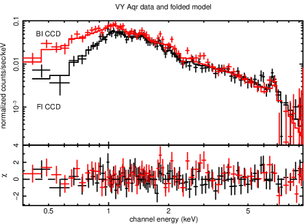
(a) VY Aqr

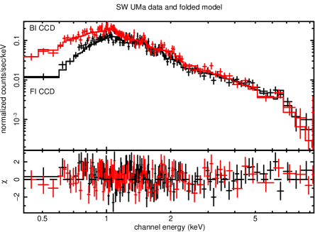
(b) SW UMa

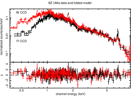
(c) BZ UMa

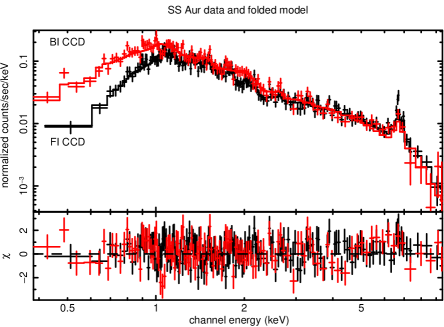
(d) SS Aur

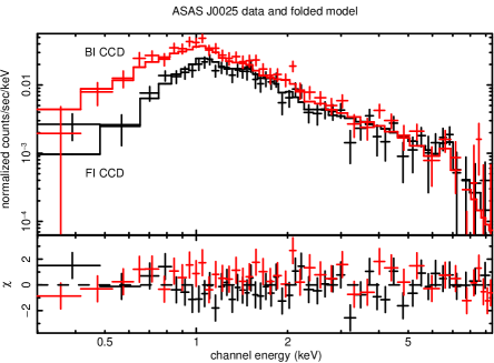
(e) ASAS J0025

Figure 1: The X-ray spectra of (a) VY Aqr, (b) SW UMa, (c) BZ UMa, (d) SS Aur, and (e) ASAS J0025 fitted with an absorbed cooling flow model and a 6.4 keV Gaussian line (upper panels). The lower panel in each figure shows the residuals. The black spectra correspond to the front-illuminated (FI) XIS0,3 and the red ones to the back-illuminated (BI) XIS1 spectra.

The measured equivalent widths of the 6.4 keV line for each source are given in Table LABEL:ev, and the results of the spectral fitting for the optically thin thermal plasma and the cooling flow models are given in Table LABEL:mekal and LABEL:mkcflow, respectively. These results show that in general, better $\chi^{2}_{\nu}$/$\nu$ values are achieved with the cooling flow model. For example, the improvement with the cooling flow model was statistically significant for SW UMa and T Leo. Fig. 1 illustrates the X-ray spectra of the new Suzaku XIS observations, i.e. VY Aqr, SW UMa, BZ UMa, SS Aur, and ASAS J0025, which have been fitted with the cooling flow model absorbed by photoelectric absorption with an added 6.4 keV Gaussian line component. Most of the X-ray spectra show that the clearest, discrete emission feature seen in the spectra of our source sample is the iron Fe K$\alpha$ complex, except in GW Lib, for which the signal-to-noise at $\sim$ 6 keV is too low for a reliable measurement.

5.1 Absorption

Since the studied sources are all within $\sim$ 200 pc, i.e., within the solar neighbourhood, the effect of interstellar absorption should be negligible. Thus, high measured absorption columns would mainly be due to intrinsic absorption, associated with the sources. For most of the sources, the measured absorption columns were typically of the order of a few $\times$ 10²⁰ cm^-2, or even lower (10¹⁹ cm^-2) which indicate low intrinsic absorption.

The highest intrinsic absorption columns are found in V893 Sco, Z Cam and HT Cas when compared to the rest of the source sample. All these three sources have partial covering absorbers $n_{H_{2}}$ with values of the order of 10²¹ – 10²² cm^-2 depending on the model. In addition to the partial covering absorber, Z Cam also has a simple absorption component with the highest $n_{H_{1}}$ value, $n_{H_{1}}$ $\sim$ 3 $\times$ 10²¹ cm^-2, within the source sample. Originally, V893 Sco was found to have high intrinsic absorption by Mukai, Zietsman & Still (2009), and has a partial X-ray eclipse, also discovered by their study. Also, according to the best-fit model of Baskill, Wheatley & Osborne (2001), Z Cam had large amounts of absorption with $n_{H}$ = 9 $\times$ 10²¹ cm^-2 during the transition state. Baskill et al. suggested that this absorption was associated with a clumpy disc wind.

5.2 Temperatures

The measured shock temperatures $kT_{max}$ seem to be correlated with the white dwarf masses (Fig. 2) as one would expect. In Fig. 2 it has been assumed that the white dwarf mass of VY Aqr is 0.8 M_⊙ (see Table LABEL:sources). ASAS J0025 is not included in Fig. 2 since the mass estimate is currently unknown. SS Cyg appears to be located in the upper right corner due to its high-mass white dwarf and thus high shock temperature. The shock temperatures, $kT_{max}$, in Fig. 2 have been derived from the spectral fits of the cooling flow model for each source. The blue dashed line in Fig. 2 represents the theoretical shock temperatures for given white dwarf masses. The radii, $R_{*}$, of the given white dwarf masses, $M_{1}$, were calculated assuming the mass-radius relation for cold, non-rotating and non-relativistic helium white dwarfs (see Pringle & Webbink, 1975)

$$R_{*}=7.7\times 10^{8}x^{0.3767-0.00605\,\log(x)}\quad(cm),$$ (2)

where $x$ = $\frac{1.44M_{\odot}}{M_{1}}$ -1. Subsequently, the theoretical shock temperatures, $T_{shock}$, for non-magnetic CVs were calculated according to Eq. 3 for optically thin gas (Frank, King & Raine, 2002)

$$T_{shock}=\frac{3}{16}\frac{GM_{1}\mu m_{H}}{kR_{*}},$$ (3)

where $m_{H}$ is the mass of a hydrogen atom, $\mu$ the mean molecular weight, and $k$ the Boltzmann constant. As it appears from Fig. 2, sources with high shock temperatures and low luminosities are not seen. This is sensible since the X-ray luminosity is proportional to $kT_{max}$ and the mass accretion rate, i.e. the normalization of the cooling flow model (Eq. 1), thus we would expect to see high shock temperatures and high luminosities. Also, due to this proportionality, we expect to see an anti-correlation between $\dot{M}$ and $kT_{max}$ which indeed is seen for example in SW UMa (Fig. 3).

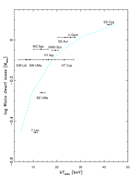
Figure 2: Mass of the white dwarf versus the shock temperature, $kT_{max}$, of the source sample with 90 per cent uncertainties for $kT_{max}$. The light blue dashed line represents the theoretical shock temperatures for given white dwarf masses. The figure does not include ASAS J0025 since a mass estimate does not currently exist for this source.

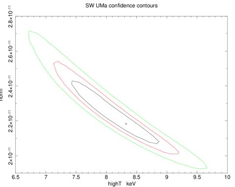
Figure 3: The 68, 90, and 99 per cent confidence contours of SW UMa for the normalisation ($\dot{M}$) versus the shock temperature $kT_{max}$ of the cooling flow model.

As it appears from Fig. 2, the white dwarf mass obtained for T Leo by Urban & Sion (2006) is only 0.35 M_⊙. This mass estimate may be unreliable, since as Lemm et al. (1993) argue, a low white dwarf mass would not allow superhumps to develop. See also Patterson et al. (2005) who refer to previous superhump studies which have shown that the mass ratio $q$ = $M_{2}/M_{1}$ has a key role in producing superhumps where $q_{crit}$ $\sim$ 0.3, although this value has not been confirmed by observational evidence.

5.3 Abundances

We found that for most of the objects in the sample the obtained abundances were sub-solar with both models. In general, the abundances seem to be dependent on the spectral model: abundances are slightly lower when the spectra are fitted with the optically thin thermal plasma model. This is due to the single temperature characteristic of the optically thin thermal plasma model, i.e. it is likely that the abundances are underestimated because the best-fit temperature usually converges close to the peak of the 6.7 keV He-like Fe K$\alpha$ emissivity, whereas the cooling flow model consists of a range of temperatures outside the peak (see Mukai, Zietsman & Still, 2009).

5.4 X-ray fluxes and luminosities

The 2–10 and bolometric 0.01–100 keV fluxes and luminosities which were derived using the cooling flow model are given in Table LABEL:fluxes. This shows that most of the 2–10 keV X-ray luminosities are concentrated around 10³⁰ erg s^-1. This is also seen in Fig. 4 which shows a histogram of the X-ray luminosities of our sample. Only one object, GW Lib, stands out with a very low luminosity (4 $\times$ 10²⁸ erg s^-1). The measured luminosity of GW Lib is consistent with the results obtained by Hilton et al. (2007). Byckling et al. (2009) showed that GW Lib was still an order of a magnitude brighter (L $\sim$ 10³⁰ erg s^-1) in X-rays during Swift observations two years after the 2007 outburst than in 2005. But since the optical magnitude had not reached the quiescence level (V $\sim$ 18) in 2009, we do not consider the Swift 2009 X-ray luminosity as the quiescent luminosity. Thus, the higher X-ray luminosity measured in the Swift data does not affect the results of this paper.

Figure 4: A histogram showing the X-ray luminosities of the source sample in 2–10 keV.

Table 6: Fluxes and luminosities in the 2–10 (absorbed) and 0.01–100 keV (unabsorbed) bands derived from the cooling flow model for each source.

Source	F(2–10 keV)	L(2–10 keV)	F(0.01–100 keV)	L(0.01–100 keV)
	x 10-12 erg cm-2 s-1	$\times$ 1030 erg s-1	x 10-12 erg cm-2 s-1	$\times$ 1030 erg s-1
BZ UMa	2.4${}^{+0.1}_{-0.2}$	14.9${}^{+10.8}_{-5.9}$	5.8	36.5
GW Lib	0.04${}^{+0.03}_{-0.01}$	0.05${}^{+0.10}_{-0.02}$	0.1	0.1
HT Cas	2.9${}^{+0.7}_{-0.4}$	6.1${}^{+4.2}_{-2.2}$	7.2	14.9
SS Aur	2.9${}^{+0.3}_{-0.3}$	9.6${}^{+2.3}_{-1.9}$	7.1	23.9
SW UMa	1.5${}^{+0.2}_{-0.1}$	4.9${}^{+2.2}_{-1.3}$	4.2	13.7
U Gem	6.9${}^{+0.3}_{-0.3}$	8.3${}^{+1.0}_{-1.0}$	17.1	20.6
T Leo	5.2${}^{+0.3}_{-0.3}$	6.4${}^{+2.3}_{-1.7}$	13.2	16.3
V893 Sco	17.3${}^{+1.1}_{-1.1}$	50.1${}^{+51.9}_{-21.4}$	45.7	133.0
VY Aqr	1.1${}^{+0.2}_{-0.2}$	1.3${}^{+0.8}_{-0.5}$	2.6	3.0
WZ Sge	3.1${}^{+1.2}_{-0.5}$	0.7${}^{+0.3}_{-0.1}$	7.7	1.8
SS Cyg	45.7${}^{+0.5}_{-0.8}$	150.0${}^{+29.0}_{-20.0}$	131.7	433.0
Z Cam	19.2${}^{+1.9}_{-2.6}$	61.6${}^{+74.4}_{-30.3}$	52.3	168.0
ASAS J0025	0.4${}^{+0.1}_{-0.1}$	1.6${}^{+3.8}_{-0.8}$	1.1	3.9

One of the sources in our sample, SS Aur, has previously been listed in the RXTE All-Sky Slew Survey catalog where it appears more luminous in X-rays than in our Suzaku observation (the RXTE flux of SS Aur in 2–10 keV is $\sim$ 1.1 $\times$ 10^-11 erg cm^-2 s^-1). We suspect that the higher flux in the RXTE observation is due to other, bright sources in the field which overestimate the flux. E.g., the ROSAT Bright Source Catalogue lists a cluster of galaxies, Abell 553, which is 53’ away from SS Aur and has a WebPIMMS estimated flux of $\sim$ 9.3 $\times$ 10^-12 erg cm^-2 s^-1 in 2–10 keV (bremsstrahlung kT = 4 keV, Galactic n_H = 1.56 $\times$ 10²¹ cm^-2 as in Ebeling et al., 1996). Thus, the higher RXTE flux of SS Aur is very likely biased by the background sources and not reliable.

5.5 The outburst of KT Per

We also analysed the Suzaku outburst data of KT Per obtained in January 2009, and report the results here. KT Per is a Z Cam type dwarf nova, and was seen as an X-ray source by the Einstein satellite in 1979 (Córdova & Mason, 1984). We employed the same models which were used for the source sample above, i.e. an absorbed optically thin thermal plasma model and an absorbed cooling flow model with an added 6.4 keV line. Both models yielded acceptable fits: $\chi_{\nu}^{2}/\nu$ = 0.97/838 (thermal plasma) and $\chi_{\nu}^{2}/\nu$ = 0.95/837 (cooling flow). Fig. 5 shows the XIS1 and the combined XIS0,3 X-ray spectra of KT Per which have been fitted with an absorbed cooling flow model with a 6.4 keV Gaussian line. The spectral fit parameters for the optically thin thermal plasma and the cooling flow models with fluxes, luminosities and fit statistics are given in Table LABEL:ktper. The luminosities given in Table LABEL:ktper are calculated for the distance of 180${}^{+36}_{-28}$ pc (Thorstensen, Lépine, & Shara, 2008). Baskill, Wheatley, & Osborne (2005) noted that cooling flow models are often a good representation of quiescent X-ray spectra of CVs (see also Mukai et al., 2003), but not outburst spectra. Baskill et al. applied the Xspec multi-temperature model cevmkl to their ASCA spectra in order to fit a range of outburst and quiescent spectra with a single simple model. We also investigated how this multi-temperature model combined with photoelectric absorption and a 6.4 keV Gaussian line would fit the outburst data of KT Per, and obtained a statistically acceptable fit: $\chi_{\nu}^{2}/\nu$ = 0.96/836, P₀ = 0.819.

Table 7: The fit parameters of KT Per derived by using an absorbed optically thin thermal plasma and absorbed cooling flow models with a 6.4 keV iron line. The errors are 90 per cent errors for one parameter of interest.

Parameter	Thermal plasma	Cooling flow
nH	14.40${}^{+1.60}_{-1.54}$	15.70${}^{+2.05}_{-1.78}$
$\times$ 1020 cm-2
kT	5.11${}^{+0.32}_{-0.31}$	12.60${}^{+1.47}_{-2.29}$
(keV)
Abundance	0.40${}^{+0.07}_{-0.07}$	0.42${}^{+0.09}_{-0.08}$
EW	52${}^{+39}_{-38}$	45${}^{+44}_{-44}$
(eV)
Flux(2–10 keV)	2.55	2.62
$\times$ 10-12 erg cm-2 s-1
Flux(0.01–100 keV)	5.60	6.19
$\times$ 10-12 erg cm-2 s-1
Luminosity(2–10 keV)	1.0	1.03
$\times$ 1031 erg s-1
Luminosity(0.01–100 keV)	2.19	2.42
$\times$ 1031 erg s-1
$\chi^{2}_{\nu}/\nu$	0.97/838	0.95/837
P0	0.730	0.819

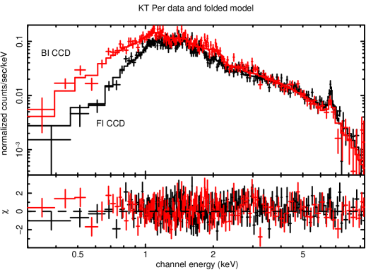
Figure 5: The X-ray spectrum of KT Per fitted with an absorbed cooling flow model and a 6.4 keV Gaussian line. The lower panel shows the residuals. The black spectrum corresponds to the front-illuminated (FI) XIS0,3 and the red one to the back-illuminated (BI) XIS1 spectrum.

5.6 Calculating the height of the X-ray emission source above the white dwarf surface

The method which is used for calculating the height of the X-ray emission source above the white dwarf, has been explained by Ishida et al. (2009) for SS Cyg. We have adopted the same method here in our work. As was explained in the beginning of Section 5, an equivalent width of up to $\sim$ 150 eV can be expected for the fluorescent Fe K$\alpha$ line at 6.4 keV. In this work, we have assumed that the reflection originates from the white dwarf surface only, thus the reflection from the accretion disc is $\Omega_{disc}$/2$\pi$ = 0. The equivalent width of 150 eV calculated by George & Fabian (1991) was assumed under the solar abundance conditions of Morrison & McCammon (1983) where [Fe/H] = 3.2 $\times$ 10^-5. We have employed the abundances of Anders & Grevesse (1989) which are the default abundance values built in the Xspec cooling flow and optically thin thermal plasma emission models. For the solar abundances of Anders & Grevesse, the [Fe/H] composition is 4.68 $\times$ 10^-5. Ishida et al. (2009), who also employed the Anders & Grevesse abundances, corrected this abundance difference (see their Eq.3) using their measured iron abundance of 0.37 $Z_{0}$. For solar abundance, the observed equivalent width of the 6.4 keV line is

$$EW_{observed} =150\times\frac{4.68\times 10^{-5}}{3.2\times 10^{-5}}\Big{(}\frac{\Omega_{WD}}{2\pi}\Big{)}Z\quad(eV)$$

$$=220\Big{(}\frac{\Omega_{WD}}{2\pi}\Big{)}Z\quad(eV),$$ (4)

where $Z$ is the measured elemental abundance in solar units $Z_{\odot}$ and $\Omega_{WD}$ the solid angle of the white dwarf viewed from the plasma of the boundary layer. In our sample, the observed equivalent widths (Table LABEL:ev) are mainly below 150 eV and this implies that the X-ray source is located at a height $h$ above the white dwarf surface. In the following, we use the values of $EW_{observed}$ and abundances calculated from the cooling flow model. As an example, the $EW_{observed}$ for SS Aur is 86 eV and the abundance is 1.0, thus Eq. 5.6 gives $\Omega_{WD}$/2$\pi$ = 0.39. If the X-ray source is point-like, the height $h$ of the X-ray source above the white dwarf of a radius $R_{WD}$ is $h$ $<$ 0.14 $R_{WD}$. As another example, we obtain $\Omega_{WD}$/2$\pi$ = 0.22 and $h$ $<$ 0.64 $R_{WD}$ for V893 Sco ($EW_{observed}$ = 45 eV, $Z$ = 0.94 Z₀).

6 Discussion

We have derived an X-ray luminosity function for 12 dwarf novae using archival Suzaku, XMM-Newton, and ASCA observations, and obtained new observations for BZ UMa, SW UMa, VY Aqr, SS Aur, V893 Sco and ASAS J0025 with Suzaku as originally, they were not available in the archive. Our results show that the 2–10 keV luminosities, presented in Table LABEL:fluxes, span a range between 4 $\times$ 10²⁸ and 1.5 $\times$ 10³² erg s^-1, and that most of the source luminosities in the sample are located within 10³⁰ erg s^-1, see Fig. 4, whereas, the X-ray luminosities of the ASCA sample by Baskill, Wheatley, & Osborne (2005) were mainly concentrated on higher luminosities between 10³¹ and 10³² erg s^-1. This difference is most likely due to the fact that we did not apply X-ray selection criteria to our sample. Also, the objects observed by ASCA were known to be X-ray bright, thus the sample of Baskill et al. is very likely biased by sources which are X-ray bright.

In order to derive the integrated X-ray luminosity function (XLF), N($>$ L), for 12 sources within a distance of d = 200 pc, we assumed that the luminosity function is characterized by a power law N($>$ L) = k(L/L_t)^-α (see Fig. 6 where the best-fit parameters $\alpha$ = -0.64 and k = 2.39 $\times$ 10^-7, corresponding to a threshold luminosity of L_t = 3 $\times$ 10³⁰ erg s^-1). The histogram illustrates the cumulative source distribution per pc³ in which a break is seen at $\sim$ 3 $\times$ 10³⁰ erg s^-1. This can be due to two possible scenarios: 1) a single $\alpha$ power law describes the luminosity function of DNe, but the sample becomes more incomplete below $\sim$ 3 $\times$ 10³⁰ erg s^-1 than it is above this limit, or 2) the shape of the true XLF of DNe is a broken power law with a break at around 3 $\times$ 10³⁰ erg s^-1. From these two scenarios, the first one is more likely since the sample contains only a few sources below $\sim$ 10³⁰ erg s^-1. Also, as was shown by, e.g., the study of Gänsicke et al. (2009), more fainter CVs, such as WZ Sge types, are expected to exist. Based on the obtained power law slope, the sample is dominated by the brighter DNe: this is probably caused by the parallax measurement method which favours optically brighter DNe which usually have high X-ray luminosities.

Figure 6: The cumulative source distribution (histogram) and the integrated power law luminosity function N($>$ L) as a function of X-ray luminosity in log L in the 2–10 keV energy band. The error bar on the top right represents a typical error on the luminosities.

When calculating the total, integrated luminosity of the sample, we restricted the calculations to the distance of 200 pc, thus excluding BZ UMa. Integrating between the luminosities of 1 $\times$ 10²⁸ and the maximum luminosity of the sample ($L_{max}$ = 1.50 $\times$ 10³² erg s^-1), yields the total integrated luminosity of 1.48 $\times$ 10³² erg s^-1, whereas the integrated luminosity between the threshold luminosity 3 $\times$ 10³⁰ and $L_{max}$ is 1.15 $\times$ 10³² erg s^-1. These two results show that there are uncertainties in the integrated luminosities, most likely caused by the small number of sources in the sample. In order to obtain more accurate value for the integrated luminosity, the power law slope ($\alpha$ = -0.64) should be better established. If the obtained slope is not far from the true power law slope of DNe in the solar neighbourhood, estimating the integrated luminosity more accurately and constraining the bright luminosity end (10³² erg s^-1) requires more DNe to be included in the sample. Since the source density at $\sim$ 10³² erg s^-1 is $\sim$ 3 $\times$ 10^-8 pc^-3 according to Fig. 6, we would need to survey within a volume of 1 $\times$ 10⁹ pc³ to find $\sim$ 30 SS Cyg -type DNe and thus find a statistically significant constraint for the brighter luminosities in the sample. This volume would correspond to a distance of $\sim$ 620 pc with a flux limit of $\sim$ 3.2 $\times$ 10^-12 erg cm^-2 s^-1.

Following this, we estimated how easy it would be to hide typical DN luminosities in the solar neighbourhood. Assuming a typical dwarf nova with a 5 keV bremsstrahlung and a low Galactic n_H = 1 $\times$ 10²⁰ cm^-2 in WebPIMMs yields a 2–10 keV flux of 5 $\times$ 10^-13 erg cm^-2 s^-1, corresponding to the ROSAT PSPC count rate of 0.04 ct s^-1 which is just below the detection limit (0.05 ct s^-1) of ROSAT PSPC (Voges et al., 1999). Thus, luminosities above 2.4 $\times$ 10³⁰ erg s^-1 within 200 pc or above 6 $\times$ 10²⁹ erg s^-1 within 100 pc should have been found by ROSAT and thus should be in the RASS. However, given that sources with luminosities of 10³⁰ erg s^-1 and below at a distance of 100 pc were too faint for the RASS, and that our XLF peaks at $\sim$ 10³⁰ erg s^-1, we conclude that there is no existing X-ray selected sample that we can use for this line of research.

How far is the total luminosity of our sample from accounting for the total CV X-ray emissivity? In order to estimate this, we calculated the absolute lower limit for the luminosity per cubic parsec volume (L_x/vol). For a distance of r = 200 pc, the volume V = 4/3 $\times$ $\pi$ $\times$ (200 pc)³ = 3.3 $\times$ 10⁷ pc³, and the total summed luminosity L_x of the sample is 2.39 $\times$ 10³² erg s^-1 (without BZ UMa). Thus, the total absolute lower limit L_x/volume = 7.24 $\times$ 10²⁴ erg s^-1 pc^-3. Normalising this value to the local stellar mass density 0.04 M_⊙ pc^-3 (Jahreiß & Wielen, 1997) yields 1.81 $\times$ 10²⁶ erg s^-1 M${}_{\odot}^{-1}$ in the 2–10 keV range. For comparison, Sazonov et al. (2006) obtained (1.1 $\pm$ 0.3) $\times$ 10²⁷ erg s^-1 M${}_{\odot}^{-1}$ (2–10 keV) for the total CV X-ray emissivity per unit stellar mass. Thus, our sample would account for $\sim$ 16 per cent of this value.

And finally, how much would our sample account for the GRXE? The Galactic Ridge X-ray emissivity estimated by Revnivtsev et al. (2006) in the 3–20 keV range was L_x/M $\sim$ (3.5 $\pm$ 0.5) $\times$ 10²⁷ erg s^-1 M${}_{\odot}^{-1}$, meaning that our sample would account for 5 per cent of the Galactic Ridge X-ray emissivity. As we estimated the X-ray emissivity of all CVs within 200 pc, we used the exponential vertical density profile

$$\rho(z)=\rho_{0}e^{|z|/h},$$ (5)

of CVs with a scale height for short period systems ($h$ = 260 pc) as in Pretorius et al. (2007b), where $z$ = $d$ sin $b$ is the perpendicular distance from the Galactic plane and $b$ Galactic latitude. Integrating Eq.5 over a sphere with a radius of 200 pc gives $\sim$ 280 as the total number of DNe within 200 pc. If the space density of DNe follows the space density of CVs as in Pretorius et al. (2007b), i.e., $\rho_{0}$ = 1.1${}^{+2.3}_{-0.7}$ $\times$ 10^-5 pc^-3, and if a typical DN has an X-ray luminosity corresponding to the mean luminosity (2 $\times$ 10³¹ erg s^-1) of our sample of 11 sources (BZ UMa excluded), then the 2–10 keV X-ray emissivity of all DNe in the solar neighbourhood would be 5.5${}^{+11.5}_{-3.5}$ $\times$ 10²⁷ erg s^-1 M${}_{\odot}^{-1}$ (these account for the uncertainty on the space density, assuming that this is the dominant source of uncertainty for the X-ray emissivity of DNe). This would account for more than 100 per cent of the GRXE emissivity. If DNe were uniformly distributed in the solar neighbourhood, the X-ray emissivity would be overestimated also in this case (by 20–30 per cent). However, in both cases, one should remember that the calculated X-ray emissivity of all DNe within 200 pc is likely overestimated by the brighter sources in our sample, thus the calculations give excess emission.

6.1 Correlations between X-ray luminosity and other parameters

In order to understand whether the X-ray luminosity and the various parameters (inclination $i$, orbital period $P_{orb}$, shock temperature $kT_{max}$ and white dwarf mass $M_{WD}$) are correlated, we carried out Spearman’s rank correlation test. Plotting X-ray luminosity versus a few of these parameters ($i$ and $P_{orb}$) shows that GW Lib seems to appear as an outlier compared to the rest of the sample (Fig. 7 and 8). Thus, to explore how the presence/absence of GW Lib affects the test results, two test cases were used: 1) GW Lib was included, and 2) GW Lib was excluded from the rest of the sample. In addition, we investigated whether a correlation between the white dwarf masses $M_{WD}$ and the shock temperatures $kT_{max}$ (Fig. 2) exists, although in this case, GW Lib seems to follow the rest of the sample, thus, carrying out test case 2) was not necessary.

Figure 7: The X-ray luminosities (2.0–10.0 keV) versus orbital periods of the source sample.

Figure 8: The X-ray luminosities (2.0–10.0 keV) versus inclinations of the source sample.

A strong correlation was found at the 99.95 per cent significance level (2.8$\sigma$) between the X-ray luminosities and orbital periods (Fig. 7) when GW Lib is included in the sample. The correlation still holds when GW Lib is excluded (significance is 99.67 per cent). Baskill, Wheatley, & Osborne (2005) noted that there was a weak correlation between the X-ray luminosities and the orbital periods in their ASCA sample, concluding that the X-ray luminosity probably also correlates with long-term mean accretion rate.

The X-ray luminosity and the inclination $i$ are not correlated in either case (Fig. 8). The correlation between these parameters was measured when the inclination of BZ UMa was set to 65^∘, and altering the inclination between 60^∘ and 75^∘ did not affect the result. Since no correlation was found, this result is in contrast with the discovery of anti-correlation between the emission measure and inclination found by van Teeseling, Beuermann, & Verbunt (1996). It is worth noting that the ROSAT bandpass was very narrow, covering only 0.1–2.4 keV where the softer X-ray emission (and more luminous emission) is probably intrinsically absorbed by the sources. In addition, an anti-correlation between the X-ray luminosity and inclination was also seen by Baskill, Wheatley, & Osborne (2005) in the ASCA sample, although, Baskill et al. noted that the inclinations might be uncertain, and this can also be the case in our sample.

Finally, the white dwarf masses $M_{WD}$ and the shock temperatures $kT_{max}$ correlate with a significance of 98.5 per cent when the mass of VY Aqr is 0.80 M_⊙, but becomes less significant (97.4 per cent) if the mass is 0.55 M_⊙. Of the rest of the parameters, i.e. the X-ray luminosity $L_{x}$ versus $kT_{max}$ and $M_{WD}$, $kT_{max}$ showed evidence of correlation with $L_{x}$ at a significance of 97.6 per cent when GW Lib was included in the sample, but $L_{x}$ and $M_{WD}$ had a much lower correlation significance (69 per cent) when including GW Lib. For the latter correlation test ($L_{x}$ versus $M_{WD}$), the result was the same with both $M_{WD}$ values for VY Aqr. Excluding GW Lib decreased the significance to 91 per cent ($L_{x}$ versus $kT_{max}$) and to 63 per cent ($L_{x}$ versus $M_{WD}$).

7 Conclusions

We have analysed the X-ray spectra of 13 dwarf novae with accurate parallax-based distance estimates, and derived the most accurate shape for the X-ray luminosity function of DNe in the 2–10 keV band to date due to accurate distance measurements and due to the fact that we did not use an X-ray selected sample.

The derived X-ray luminosities are located between $\sim$ 10²⁸–10³² erg s^-1, showing a peak at $\sim$ 10³⁰ erg s^-1. Thus, we have obtained peak luminosities which are lower compared to other previous studies of CV luminosity functions. The shape of the X-ray luminosity function of the source sample suggests that the two following scenarios are possible: 1) the sample can be described by a power law with a single $\alpha$ slope, but the sample becomes more incomplete below $\sim$ 3 $\times$ 10³⁰ erg s^-1 than it is above this limit, or, 2) the shape of the real X-ray luminosity function of dwarf novae is a broken power law with a break at around 3 $\times$ 10³⁰ erg s^-1.

The integrated luminosity between 1 $\times$ 10²⁸ erg s^-1 and the maximum luminosity of the sample, 1.50 $\times$ 10³² erg s^-1, is 1.48 $\times$ 10³² erg s^-1. In order to better constrain the integrated luminosity and the slope of the X-ray luminosity function, more dwarf novae need to be included in the sample. Thus, we suggest more future X-ray imaging observations of dwarf novae in the 2–10 keV band with accurate distance measurements. The total X-ray emissivity of the sample within a radius of 200 pc is 1.81 $\times$ 10²⁶ erg s^-1 M${}^{-1}_{\odot}$ (2–10 keV). This accounts for $\sim$ 16 per cent of the total X-ray emissivity of CVs as estimated by Sazonov et al. (2006), and $\sim$ 5 per cent of the Galactic Ridge X-ray emissivity.

The X-ray luminosities and the inclinations of our sample do not show anti-correlation which has been seen in other previous correlation studies, but a strong correlation is seen between the X-ray luminosities and the orbital periods. Also, evidence for a correlation between the white dwarf masses and the shock temperatures exists. In the future, larger dwarf nova samples are needed in order to confirm these results.

References

- Arnaud (1996) Arnaud K.A., 1996, ASP Conf. Ser. Vol. 101, Astronomical Data Analysis Software and Systems V. Astron. Soc. Pac., San Francisco, p. 17
- Anders & Grevesse (1989) Anders E., Grevesse N., 1989, Geochim. Cosmochim. Acta, 53, 197
- Baskill, Wheatley & Osborne (2001) Baskill D., Wheatley P. J., Osborne J. P., 2001, MNRAS, 328, 71
- Baskill, Wheatley, & Osborne (2005) Baskill D., Wheatley P. J., Osborne J. P., 2005, MNRAS, 357, 626
- Byckling et al. (2009) Byckling K., Osborne J. P., Wheatley P. J., Wynn G. A., Beardmore A., Braito V., Mukai K., West R., 2009, MNRAS, 399, 1576
- Córdova & Mason (1984) Córdova F.A., Mason K.O., 1984, MNRAS, 206, 879
- Done & Osborne (1997) Done C., Osborne J. P., 1997, MNRAS, 288, 649
- Ebeling et al. (1996) Ebeling H., Voges W., Böhringer H., Edge A. C., Huchra J. P., Briel U. G., 1996, MNRAS, 281, 799
- Ebisawa et al. (2001) Ebisawa K., Maeda Y., Kaneda H., Yamauchi S., 2001, Science, 293, 1633
- Frank, King & Raine (2002) Frank J., King A., Raine D., 2002, Accretion Power in Astrophysics, CUP, p. 156
- Friend, Connon-Smith & Jones (1990) Friend M. T., Connon-Smith, R., Jones, D. H. P., 1990, MNRAS, 246, 654
- George & Fabian (1991) George I. M., Fabian, A. C., 1991, MNRAS, 249, 352
- Gänsicke et al. (2009) Gänsicke B. T. et al., 2009, MNRAS, 397, 2170
- Harrison et al. (1999) Harrison T. E., McNamara B. J., Szkody P., McArthur B. E., Benedict G. F., Klemola A. R., Gilliland R. L., 1999, ApJ, 515, 93
- Harrison et al. (2004) Harrison T. E., Johnson, J. J., McArthur, B. E., Benedict, G. F., Szkody, P., Howell, S. B., Gelino, D. M., 2004, AJ, 127, 460
- Hilton et al. (2007) Hilton E.J., Szkody P., Mukadam A., Mukai K., Hellier C., van Zyl L., Homer L., 2007, AJ, 134, 1503
- Horne, Wood & Stiening (1991) Horne K., Wood J. H., Stiening R. F., 1991, ApJ, 378, 271
- Howell, Rappaport & Politano (1997) Howell S. B., Rappaport S., Politano M., 1997, MNRAS, 287, 929
- Ishida et al. (2009) Ishida M., Okada S., Hayashi T., Nakamura R., Terada Y., Mukai K., Hamaguchi K., 2009, PASJ, 61, S77
- Kolb (1993) Kolb U., 1993., A&A, 271, 149
- Jahreiß & Wielen (1997) Jahreiß H., Wielen R., 1997, ESA SP-402: Hipparcos - Venice ’97, 675
- Jansen et al. (2001) Jansen F. et al., 2001, A&A, 365, 1
- Lasota (2001) Lasota J.-P., 2001, NewAR, 45, 449
- Lemm et al. (1993) Lemm K., Patterson J., Thomas G., Skillman D. R., 1993, PASP, 105, 1120
- Liedahl, Osterheld & Goldstein (1995) Liedahl D. A., Osterheld A. L., Goldstein W. H., 1995, ApJ, 438, L115
- Mason et al. (2001) Mason E., Skidmore W., Howell S.B., Mennickent R.E., 2001, ApJ, 563, 351
- Mewe, Lemen & van den Oord (1986) Mewe R., Lemen J. R., van den Oord G. H. J., 1986, A&A, 65, 511
- Mitsuda et al. (2007) Mitsuda K. et al., 2007, PASJ, 59, 1
- Mukai & Shiokawa (1993) Mukai K., Shiokawa K., 1993, ApJ, 418, 863
- Mukai et al. (1997) Mukai K., Wood J. H., Naylor T., Schlegel E. M., Swank J. H., 1997, ApJ, 475, 812
- Mukai et al. (2003) Mukai K., Kinkhabwala A., Peterson J. R., Kahn S.M., Paerels F., 2003, ApJ, 586, L77
- Mukai, Zietsman & Still (2009) Mukai K., Zietsman E., Still M., 2009, ApJ, 707, 652
- Mushotzky & Szymkowiak (1988) Mushotzky R. F., Szymkowiak A. E., 1988, in Cooling Flows in Clusters and Galaxies, ed. A.C. Fabian, (Dordrecht:Kluwer), 53
- Morrison & McCammon (1983) Morrison R., McCammon D., 1983, ApJ, 270, 119
- Pandel et al. (2005) Pandel D., Córdova F. A., Mason K. O., Priedhorsky W. C., 2005, ApJ, 626, 396
- Patterson (1984) Patterson J., 1984, ApJS, 54, 443
- Patterson et al. (2005) Patterson J., Kemp J., Harvey D. et al., 2005, PASP, 117, 1204
- Pretorius, Knigge & Kolb (2007a) Pretorius M. L., Knigge C., Kolb U., 2007a, MNRAS, 374, 1495
- Pretorius et al. (2007b) Pretorius M. L., Knigge C., O’Donoghue D., Henry J. P., Gioia I. M., Mullis C. R., 2007b, MNRAS, 382, 1279
- Pringle & Webbink (1975) Pringle, J. E., Webbink, R. F., 1975, MNRAS, 172, 493
- Pringle (1977) Pringle J. E., 1977, MNRAS, 178, 195
- Pringle & Savonije (1979) Pringle J. E., Savonije G. J., 1979, MNRAS, 187, 777
- Revnivtsev et al. (2006) Revnivtsev M., Sazonov S., Gilfanov M., Churazov E., Sunyaev R., 2006, A&A, 452, 169
- Revnivtsev, Vikhlinin & Sazonov (2007) Revnivtsev M., Vikhlinin A., Sazonov S., 2007, A&A, 473, 857
- Revnivtsev et al. (2008) Revnivtsev M., Sazonov S., Krivonos R., Ritter H., Sunyaev R., 2008, A&A, 489, 1121
- Revnivtsev et al. (2009) Revnivtsev M., Sazonov S., Churazov E., Forman W., Vikhlinin A., Sunyaev R., 2009, Nature, 458, 1142
- Ritter & Kolb (2003) Ritter H., Kolb U., 2003, A&A, 404, 301 (update RKcat7.10)
- Sazonov et al. (2006) Sazonov S., Revnivtsev M., Gilfanov M., Churazov E., Sunyaev R., 2006, A&A, 450, 117
- Scargle (1982) Scargle J. D., 1982, ApJ, 263, 835
- Tanaka, Inoue & Holt (1994) Tanaka Y., Inoue H., Holt S. S., 1994, PASJ, 46, L37
- Templeton et al. (2006) Templeton M. R. et al., 2006, PASP, 118, 236
- Thorstensen (2003) Thorstensen J. R., 2003, AJ, 126, 3017
- Thorstensen, Lépine, & Shara (2008) Thorstensen J. R., Lépine S., Shara M., 2008, AJ, 136, 2107
- Urban & Sion (2006) Urban J.A., Sion M.E., 2006, ApJ, 642, 1029
- van Teeseling, Beuermann, & Verbunt (1996) van Teeseling A., Beuermann K., Verbunt F., 1996, ApJ, 315, 467
- Voges et al. (1999) Voges W. et al., 1999, A&A, 349, 389
- Warwick et al. (1985) Warwick R. S., Turner M. J. L., Watson M. G., Willingale R., 1985, Nature, 317, 218
- Wheatley et al. (1996) Wheatley P. J., Verbunt F., Belloni T., Watson M. G., Naylor T., Ishida M., Duck S. R., Pfeffermann E., 1996, A&A, 307, 137
- Worrall et al. (1982) Worrall D. M., Marshall F. E., Boldt E. A., Swank J. H., 1982, ApJ, 255, 111