Maximum Distance Between the Leader and the Laggard for Three Brownian Walkers

Abstract

We consider three independent Brownian walkers moving on a line. The process terminates when the left-most walker (the ‘Leader’) meets either of the other two walkers. For arbitrary values of the diffusion constants $D_{1}$ (the Leader), $D_{2}$ and $D_{3}$ of the three walkers, we compute the probability distribution $P(m|y_{2},y_{3})$ of the maximum distance $m$ between the Leader and the current right-most particle (the ‘Laggard’) during the process, where $y_{2}$ and $y_{3}$ are the initial distances between the leader and the other two walkers. The result has, for large $m$, the form $P(m|y_{2},y_{3})\sim A(y_{2},y_{3})\,m^{-\delta}$, where $\delta=(2\pi-\theta)/(\pi-\theta)$ and $\theta=\cos^{-1}(D_{1}/\sqrt{(D_{1}+D_{2})(D_{1}+D_{3})}$. The amplitude $A(y_{2},y_{3})$ is also determined exactly.

I Introduction

The unions of reactions of three diffusing particles (i.e. three Brownian walkers) have been much studied in the literature RednerBook . Such systems are often amenable to exact solution, even for arbitrary values of the diffusion constants $D_{1}$, $D_{2}$, $D_{3}$, of the particles, whereas systems with more than three particles are not analytically tractable (one exception being the case when the particles are mutually annihilating, i.e. ‘vicious walkers’, with equal diffusion constants FisherHuse ). An example of the type of three-particle problem that can be exactly solved is the computation of the probability that the left-most particle (with diffusion constant $D_{1}$) has not been touched by either of the other two particles up to time $t$. This probability has a power-law decay, $P\sim t^{-\theta_{1}}$, with RednerBook ; benAvraham ; FisherGelfand ; benAvraham2

$$\theta_{1}=\frac{\pi}{2(\pi-\theta)}$$ (1)

where

$$\theta=\cos^{-1}\left[\frac{D_{1}}{\sqrt{(D_{1}+D_{2})(D_{1}+D_{3})}}\right].$$ (2)

In this paper we consider a related aspect of the three-particle system that has not been addressed so far. We define the initially left-most of the three particles to be the ‘Leader’, and the right-most of the remaining two particles to be the ‘Laggard’ (the Leader-Laggard terminology was introduced by ben Avraham et al. benAvraham2 ), and we again consider processes which terminate when the Leader is touched by either of the other two particles. We compute the probability distribution, over this set of processes (with given initial conditions for the particle locations) of the maximum distance, $m$, between the Leader and the Laggard. We find that this probability distribution has a power-law tail of the form $m^{-\delta}$, where $\delta$ is a nontrivial function of the walker diffusion constants $D_{1}$, $D_{2}$ and $D_{3}$. We note that for the special case $D_{1}=0$, this distribution of the maximal distance between the Leader and the Laggard was recently computed for arbitrary $N\geq 1$ independent particles KMR . However, for $D_{1}>0$, it is not easy to generalise this method for arbitrary $N$ and in this paper we show that the exact solution even for the $N=3$ case is highly nontrivial.

Thus we consider three Brownian particles on a line with positions $\{x_{1}(t),x_{2}(t),x_{3}(t)\}$ that evolve independently with time according to the Langevin equations

$$\frac{dx_{i}}{dt}=\eta_{i}(t)$$ (3)

where $\eta_{i}(t)$ ($i=1$, $2$ or $3$) are independent Gaussian white noises with zero mean $\langle\eta_{i}(t)\rangle=0$ and the two-time correlator, $\langle\eta_{i}(t)\eta_{j}(t^{\prime})\rangle=2D_{i}\delta_{i,j}\delta(t-t^{\prime})$. Thus $D_{i}$ denotes the diffusion constant of the $i$-th particle. Let the initial positions of the three particles be denoted by $x_{1}(0)=x_{1}$, $x_{2}(0)=x_{2}$ and $x_{3}(0)=x_{3}$ where $x_{1}\leq x_{2}\leq x_{3}$ (see Fig. 1).

Let $y_{2}(t)=x_{2}(t)-x_{1}(t)$ denote the separation at time $t$ between the first and the second particle. Similarly $y_{3}(t)=x_{3}(t)-x_{1}(t)$ denotes the separation at time $t$ between the first and the third particle. These relative coordinates start respectively from their initial values $y_{2}(0)=y_{2}=x_{2}-x_{1}\geq 0$ and $y_{3}(0)=y_{3}=x_{3}-x_{1}$ (see Fig. 1), and subsequently evolve in time via

$$\frac{dy_{2}}{dt} = \eta_{2}(t)-\eta_{1}(t)=\xi_{2}(t)$$ (4)

$$\frac{dy_{3}}{dt} = \eta_{3}(t)-\eta_{1}(t)=\xi_{3}(t)$$ (5)

where the two noises $\xi_{2}(t)$ and $\xi_{3}(t)$ are now correlated for $D_{1}>0$. Clearly $\langle\xi_{2}(t)\rangle=\langle\xi_{3}(t)\rangle=0$, while the two-time correlators are given by

$$\langle\xi_{2}(t)\xi_{2}(t^{\prime})\rangle = 2(D_{1}+D_{2})\delta(t-t^{\prime}),$$ (6)

$$\langle\xi_{3}(t)\xi_{3}(t^{\prime})\rangle = 2(D_{1}+D_{3})\delta(t-t^{\prime}),$$ (7)

$$\langle\xi_{2}(t)\xi_{3}(t^{\prime})\rangle = 2D_{1}\delta(t-t^{\prime}).$$ (8)

Let $z(t)={\rm max}\left(y_{2}(t),y_{3}(t)\right)$ denote the span of this $3$-particle process at time $t$, i.e., $z(t)$ denotes the distance at time $t$ between the left-most (the Leader) and the right-most (the Laggard) particles. We stop the process at a stopping time $t_{s}$ when the leader meets, for the first time, any of the other two particles (see Fig. 1 for an example of a realization of the process).

Let

$$m=\max_{0\leq t\leq t_{s}}\left[z(t)\right]$$ (9)

denote the maximum value of the span till the stopping time $t_{s}$. Note that both $t_{s}$ and $m$ change from one realization of the process to another. These two random variables are clearly correlated. Here we are interested in the probability distribution (marginal) of $m$ only, i.e. , $P(m|y_{2},y_{3})$ given the initial separations $y_{2}$ and $y_{3}$. We will show that $P(m|y_{2},y_{3})$ has a power law tail for large $m$

$$P(m|y_{2},y_{3})\simeq\frac{A(y_{2},y_{3})}{m^{\delta}}$$ (10)

where the exponent $\delta$ depends continuously on the three diffusion constants $D_{1}$, $D_{2}$ and $D_{3}$ and has the following exact expression

$$\delta=\frac{2\pi-\theta}{\pi-\theta}\ ,$$ (11)

where $\theta$ is given by Eq. (2)

We also compute the amplitude $A(y_{2},y_{3})$ of this power law decay exactly. This amplitude is evidently a symmetric function of $y_{2}$ and $y_{3}$ but its explicit expression turns out to be rather nontrivial.

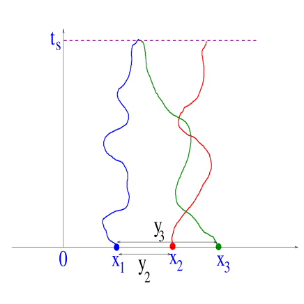
Figure 1: The trajectories of $3$ independent Brownian walkers with initial positions $x_{1}$, $x_{2}$ and $x_{3}$. The process stops at the stopping time $t_{s}$ when the leftmost (blue) particle meets any other particle, such as the third (green) particle in the figure.

II Derivation of the Result

To derive our result, it turns out to be more convenient to consider the cumulative distribution of the maximum $m$ denoted by

$$F(y_{2},y_{3}|L)=\int_{0}^{L}P(m|y_{2},y_{3})\,dm.$$ (12)

Thus $F(y_{2},y_{3}|L)$ denotes the probability that the maximum span does not exceed $L$ till the stopping time $t_{s}$, given the initial separations $y_{2}$ and $y_{3}$. The idea is to write down a backward differential equation (Backward Fokker-Planck equation) for $F(y_{2},y_{3}|L)$, treating the initial separations $y_{2}$ and $y_{3}$ as the independent variables. To do this, we consider a typical evolution of the joint process $\{y_{2}(t),y_{3}(t)\}$ via the Langevin equations (4) and (5), starting from the initial values $\{y_{2},y_{3}\}$. Let us split the full time interval $[0,t_{s}]$ of the evolution into two parts: over an initial infinitesimal time window $[0,\Delta t]$ where the joint process $\{y_{2}(t),y_{3}(t)\}$ evolves from its initial value $\{y_{2},y_{3}\}$ to the new value $\{y_{2}+\Delta y_{2},y_{3}+\Delta y_{3}\}$, where

$$\Delta y_{i}=\int_{0}^{\Delta t}\xi_{i}(t)dt\ \ \ \ (i=2,3)\ ,$$ (13)

and a subsequent interval $[\Delta t,t_{s}]$ where the process evolves starting from its ‘new’ initial position $\{y_{2}+\Delta y_{2},y_{3}+\Delta y_{3}\}$. Using the Markov property of the evolution, it then follows that

$$F(y_{2},y_{3}|L)=\langle F\left(y_{2}+\Delta y_{2},y_{3}+\Delta y_{3}|L\right)\rangle$$ (14)

where the angled brackets denotes the average over the initial displacements $\Delta y_{2}$ and $\Delta y_{3}$.

We next expand the right-hand side of Eq. (14) in a Taylor series in $\Delta t$ (to first order in $\Delta t)$ using (i) $\langle\Delta y_{i}\rangle=0$ (for $i=2,3$) and (ii) the following covariances (which follow from the delta correlators in Eqs. (6), (7) and (8))

$$\langle(\Delta y_{2})^{2}\rangle = 2\,(D_{1}+D_{2})\Delta t$$ (15)

$$\langle(\Delta y_{3})^{2}\rangle = 2\,(D_{1}+D_{3})\Delta t$$ (16)

$$\langle(\Delta y_{2}\,\Delta y_{3})\rangle = 2D_{1}\,\Delta t.$$ (17)

Keeping only terms of $O(\Delta t)$ then gives us the following partial differential equation for $F(y_{2},y_{3}|L)$:

$$(D_{1}+D_{2})\frac{\partial^{2}F}{\partial y_{2}^{2}}+(D_{1}+D_{3})\frac{\partial^{2}F}{\partial y_{3}^{2}}+2D_{1}\frac{\partial^{2}F}{\partial y_{2}\partial y_{3}}=0.$$ (18)

Note that the information that the process stops at a certain stopping time $t_{s}$ is actually captured only through the boundary conditions. Eq. (18) holds over the square $0\leq y_{2}\leq L$ and $0\leq y_{3}\leq L$ in the two dimensional $(y_{2},y_{3})$ plane with the following boundary conditions

$$F(y_{2}=0,y_{3}|L) = 1$$ (19)

$$F(y_{2},y_{3}=0|L) = 1$$ (20)

$$F(y_{2}=L,y_{3}|L) = 0$$ (21)

$$F(y_{2},y_{3}=L|L) = 0.$$ (22)

For example, if the initial separation $y_{2}=0$ and $0\leq y_{3}\leq L$, then the process stops immediately, i.e., $t_{s}=0$, since the second particle has already hit the leftmost particle. Clearly then the maximum $m=y_{3}$ which, with probability $1$, is less than or equal to $L$. Hence the boundary condition (19). By symmetry, (20) follows. In contrast, if initially say $y_{2}=L$ and $0\leq y_{3}\leq L$, clearly the initial value of $m$ is already $L$. So, the probability that $m$ will stay below $L$ subsequently is clearly $0$, indicating the boundary condition (21). By symmetry, one then has (22). So, the technical challenge is now to solve the partial differential equation (18) inside the square $[0,L]\times[0,L]$ with the above boundary conditions in Eqs. (19)-(22).

To proceed, we make a linear transformation that gets rid of the cross term in Eq. (18). In other words, we diagonalize the covariance matrix. It turns out that a linear transformation that does the job is given by

$$W_{2} = \frac{1}{\sqrt{2+\gamma}}\left(\frac{y_{2}}{\sqrt{D_{1}+D_{2}}}+\frac{y_{3}}{\sqrt{D_{1}+D_{3}}}\right)$$ (23)

$$W_{3} = \frac{1}{\sqrt{2-\gamma}}\left(-\frac{y_{2}}{\sqrt{D_{1}+D_{2}}}+\frac{y_{3}}{\sqrt{D_{1}+D_{3}}}\right)$$ (24)

where

$$\gamma=\frac{2D_{1}}{\sqrt{(D_{1}+D_{2})(D_{1}+D_{3})}}.$$ (25)

It is easy to see that $0\leq\gamma\leq 2$ for all $D_{1}\geq 0$, $D_{2}\geq 0$ and $D_{3}\geq 0$. Note also that exchanging $y_{2}$ and $y_{3}$ and also $D_{2}$ and $D_{3}$, is equivalent to letting $W_{2}\to W_{2}$ and $W_{3}\to-W_{3}$.

In terms of these new variables $(W_{2},W_{3})$, Eq. (18) becomes Laplace’s equation

$$\frac{\partial^{2}F}{\partial W_{2}^{2}}+\frac{\partial^{2}F}{\partial W_{3}^{2}}=0.$$ (26)

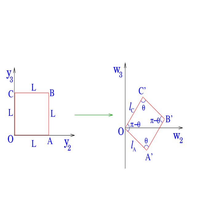
Figure 2: The linear transformation in Eqs. (23) and (24) from $(y_{2},y_{3})$ to the $(W_{2},W_{3})$ plane consists of rotation and stretching. The square $[0,L]\times[0,L]$ with vertices $0$, $A$, $B$ and $C$ in the $(y_{2},y_{3})$ plane transforms to a parallelogram with vertices $O$, $A^{\prime}$, $B^{\prime}$ and $C^{\prime}$ in the $(W_{2},W_{3})$ plane.

The original square $[0,L]\times[0,L]$ in the $(y_{2},y_{3})$ plane transforms into a parallelogram in the $(W_{2},W_{3})$ plane under the linear transformation in Eqs. (23) and (24) (see Fig. 2). The vertices $(O,A,B,C)\to(O,A^{\prime},B^{\prime},C^{\prime})$ under this transformation. It is easy to check that the lengths of the edges of the parallelogram are given by

$$l_{OA^{\prime}} = l_{B^{\prime}C^{\prime}}=l_{A}=\frac{2L}{\sqrt{(4-\gamma^{2})(D_{1}+D_{2})}}$$ (27)

$$l_{OC^{\prime}} = l_{A^{\prime}B^{\prime}}=l_{C}=\frac{2L}{\sqrt{(4-\gamma^{2})(D_{1}+D_{3})}}.$$ (28)

The angle $\theta$ in Fig. (2) can be easily computed also

$$\cos\theta=\frac{\gamma}{2}$$ (29)

where $\gamma$ is given in Eq. (25). Since $0\leq\gamma\leq 2$, it follows that $0\leq\theta\leq\pi/2$.

Laplace’s equation (26) holds inside this parallelogram in the $(W_{2},W_{3})$ plane with the boundary conditions: $F$=1 along the edges $OA^{\prime}$ and $OC^{\prime}$ and $F=0$ along the edges $A^{\prime}B^{\prime}$ and $B^{\prime}C^{\prime}$. To find the solution, we use a conformal transformation $W(z)$ that maps the polygon in the complex $W$ plane to an upper half complex $z$ plane. The conformal mapping that does this is known as the Schwarz-Christoffel transformation.

III The Schwarz-Christoffel Transformation

Consider a polygon (see Fig. (3)) in the $W$ plane having $n$ vertices at $\{w_{1},w_{2},\ldots,w_{n}\}$ with corresponding interior angles $\{\alpha_{1},\alpha_{2},\ldots,\alpha_{n}\}$. Let the points $\{w_{1},w_{2},\ldots,w_{n}\}$ map respectively into points $\{x_{1},x_{2},\ldots,x_{n}\}$ on the real axis of the $z$ plane. The Schwarz-Christoffel transformation $W=W(z)$ that maps the interior $R$ of the polygon in the $W$ plane on to the upper half $R^{\prime}$ of the $z$ plane, and the boundary of the polygon on to the real axis is given by

$$\frac{dW}{dz}=A(z-x_{1})^{\alpha_{1}/\pi-1}(z-x_{2})^{\alpha_{2}/\pi-1}\ldots(z-x_{n})^{\alpha_{N}/\pi-1}$$ (30)

where $A$ is an arbitrary complex constant. Any three of the points $\{x_{1},x_{2},\ldots,x_{n}\}$ can be chosen at will and it is convenient to choose one point, say $x_{n}$, at infinity in which case the last factor in Eq. (30) involving $x_{n}$ is not present.

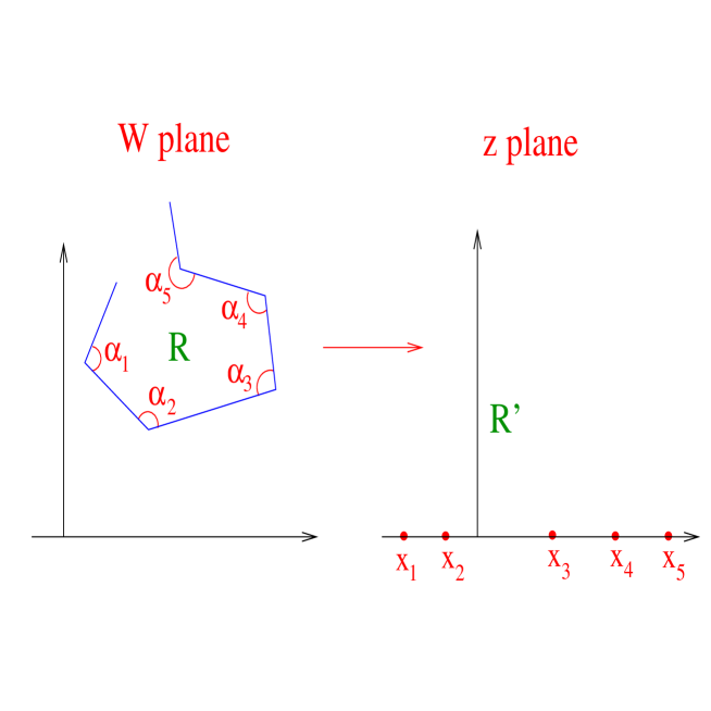
Figure 3: The Schwarz-Christoffel transformation that maps the interior $R$ of a polygon in the complex $W$ plane on to the upper half plane $R^{\prime}$ in the complex $z$ plane. The boundary of the polygon in the $W$ plane maps onto the real axis in the $z$ plane.

In our problem, we have a parallelogram in the complex $W$ plane (Fig. 2) with four vertices at $O$, $A^{\prime}$, $B^{\prime}$ and $C^{\prime}$. We choose three points $x_{1}=-a$ (image of $C^{\prime}$), $x_{2}=0$ (image of $O$) and $x_{3}=1$ (image of $A^{\prime}$) and also choose the image of $B^{\prime}$ to be at infinity (see Fig. (4)). The Schwarz-Christoffel transformation in Eq. (30) then can then be written as

$$\frac{dW}{dz}=A(a+z)^{\theta/\pi-1}z^{-\theta/\pi}(1-z)^{\theta/\pi-1}$$ (31)

where $A$ is still an arbitrary constant. Integrating, and using the fact that $W(0)=0$, we get

$$W(z)=W_{2}+iW_{3}=A\int_{0}^{z}t^{-\theta/\pi}\,\left[(a+t)(1-t)\right]^{\theta/\pi-1}\,dt.$$ (32)

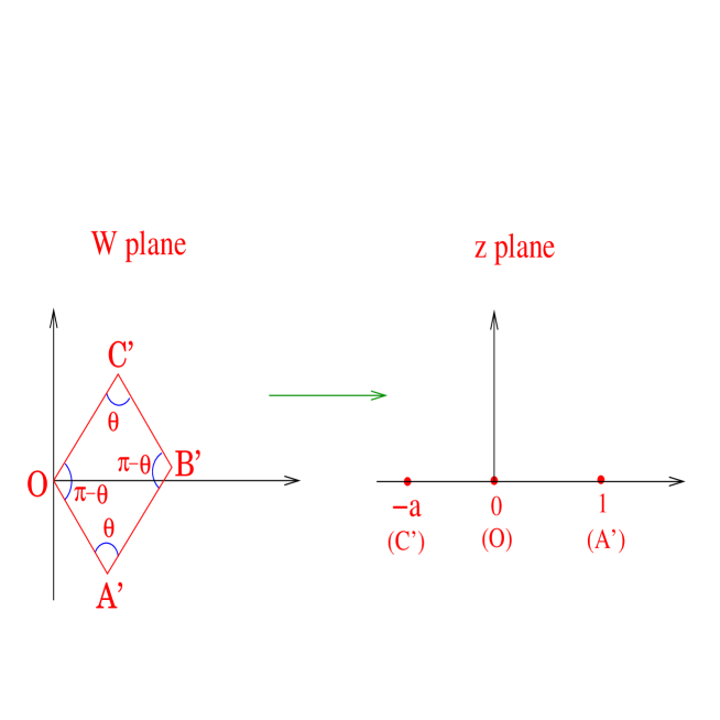
Figure 4: Under the Schwarz-Christoffel transformation the interior $R$ of the parallelogram in the complex $W$ plane maps on to the upper half plane in the complex $z$ plane. Under this transformation, The boundary of the polygon in the $W$ plane maps onto the real axis in the $z$ plane. The four vertices $C^{\prime}$, $O$, $A^{\prime}$ and $B^{\prime}$ have their respective images on the real axis of the $z$ plane at $-a$, $0$, $1$ and $\infty$.

The unknown constants $A$ and the coordinate $a$ in Eq. (32) are determined as follows. In the complex $W=W_{2}+iW_{3}$ plane, the coordinates of the vertices $A^{\prime}$ and $C^{\prime}$ are easily determined from the parallelogram in Fig. (2). They are respectively: $A^{\prime}=\left(L/\sqrt{(2+\gamma)(D_{1}+D_{2})},-L/\sqrt{(2-\gamma)(D_{1}+D_{2})}\right)$ and $C^{\prime}=\left(L/\sqrt{(2+\gamma)(D_{1}+D_{3})},L/\sqrt{(2-\gamma)(D_{1}+D_{3})}\right)$. Under the transformation $W(z)$ they get mapped to the real $z$ axis with coordinates $1$ and $-a$ respectively. Hence we get

$$W(1) = \frac{L}{\sqrt{(2+\gamma)(D_{1}+D_{2})}}-i\,\frac{L}{\sqrt{(2-\gamma)(D_{1}+D_{2})}}=A\int_{0}^{1}t^{-\theta/\pi}\,\left[(a+t)(1-t)\right]^{\theta/\pi-1}\,dt$$ (33)

$$W(-a) = \frac{L}{\sqrt{(2+\gamma)(D_{1}+D_{3})}}+i\,\frac{L}{\sqrt{(2-\gamma)(D_{1}+D_{3})}}=A\int_{0}^{-a}t^{-\theta/\pi}\,\left[(a+t)(1-t)\right]^{\theta/\pi-1}\,dt$$ (34)

The integrals can be organized in a uniform way by defining a function

$$h(a)=\int_{0}^{1}t^{-\theta/\pi}\,\left[(1+a\,t)(1-t)\right]^{\theta/\pi-1}\,dt$$ (35)

in terms of which

$$\frac{L}{\sqrt{(2+\gamma)(D_{1}+D_{2})}}-i\,\frac{L}{\sqrt{(2-\gamma)(D_{1}+D_{2})}} = Aa^{\theta/\pi-1}h(1/a)$$ (36)

$$\frac{L}{\sqrt{(2+\gamma)(D_{1}+D_{3})}}+i\,\frac{L}{\sqrt{(2-\gamma)(D_{1}+D_{3})}} = -Ae^{-i\theta}h(a).$$ (37)

Writing $A=A_{1}+iA_{2}$ and matching the real and imaginary parts determines $A_{1}$ and $A_{2}$ as

$$A_{1} = \frac{1}{h(a)}\frac{L}{\sqrt{(2+\gamma)(D_{1}+D_{3})}}$$ (38)

$$A_{2} = -\frac{1}{h(a)}\frac{L}{\sqrt{(2-\gamma)(D_{1}+D_{3})}}.$$ (39)

This also determines $a$ via the relation

$$a^{\theta/\pi-1}\,\frac{h(1/a)}{h(a)}=\sqrt{\frac{D_{1}+D_{3}}{D_{1}+D_{2}}}.$$ (40)

Note that under the exchange $2\rightleftarrows 3$, $a\rightleftarrows 1/a$.

Writing $A=A_{1}+iA_{2}=|A|e^{i\beta}$, it is easy to check that

$$|A|=\frac{1}{h(a)}\frac{2L}{\sqrt{(4-\gamma^{2})(D_{1}+D_{3})}}$$ (41)

which, using Eq. (40) can be written in a symmetrized form

$$|A|=\frac{2La^{(\pi-\theta)/2\pi}}{\left[(4-\gamma^{2})\,h(a)\,h(1/a)\,\sqrt{(D_{1}+D_{2})(D_{1}+D_{3})}\right]^{1/2}}.$$ (42)

The phase $\beta$ is given by, $\tan\beta=A_{2}/A_{1}=-\sqrt{(2+\gamma)/(2-\gamma)}$. Using $\cos\theta=\gamma/2$, one then finds

$$\beta=\frac{\theta-\pi}{2}.$$ (43)

The knowledge of $A=|A|e^{i\beta}$ and $a$ (via Eq. (40)) then fully determines the conformal transformation $W(z)$ in Eq. (32).

Once we have determined the appropriate conformal transformation in (32), we then need to solve Laplace’s equation $\nabla^{2}F=0$ in the upper half complex $z$ plane (note that the Laplace’s equation remains invariant under conformal transformation). The appropriate boundary conditions on the real axis of the $z$ plane read: $F(x,0)=0$ for $x<-a$ and $x>1$ and $F(x,0)=1$ for $-a\leq x\leq 1$. The solution of the Laplace’s equation in the upper half $z$ plane can be written down explicitly in terms of the boundary values by using Poisson’s formula

$$F(x,y)=\frac{y}{\pi}\int_{-\infty}^{\infty}\frac{F(x^{\prime},0)dx^{\prime}}{\left[y^{2}+(x-x^{\prime})^{2}\right]}.$$ (44)

Using our boundary conditions mentioned above and performing the integral we get the explicit solution in the complex $z$ plane

$$F(z)=F(x,y)=\frac{1}{\pi}\left[\tan^{-1}\left(\frac{x+a}{y}\right)-\tan^{-1}\left(\frac{x-1}{y}\right)\right].$$ (45)

To obtain the solution in terms of the original coordinates $(y_{2},y_{3})$, we need to express $(x,y)$ in terms of $(W_{2},W_{3})$ (or equivalently $(y_{2},y_{3})$) using Eqs. (23) and (24), and then use the inverse of the conformal transformation $W(z)$ in Eq. (32). This is rather tedious and far from illuminating. Instead in the following section, we derive the asymptotic solution for the distribution of the maximum for large $L$. In this asymptotic limit, it turns out that one can explicitly invert the conformal transformation.

IV Large $L$ limit: the tail of the maximum distribution

Returning to the original cumulative distribution $F(y_{2},y_{3}|L)$ of the maximum, $m$, we note that the $L$ dependence can be absorbed by rescaling the initial separations $y_{2}\to y_{2}/L$ and $y_{3}\to y_{3}/L$. In other words, the distribution is only a function of the dimensionless variables $z_{2}=y_{2}/L$ and $z_{3}=y_{3}/L$

$$F(y_{2},y_{3}|L)=F(z_{2}=y_{2}/L,z_{3}=y_{3}/L).$$ (46)

This means that the limit $L\to\infty$ is equivalent to taking limits $y_{2}\to 0$ and $y_{3}\to 0$, since $L$ always appears through the scaling combinations $y_{2}/L$ and $y_{3}/L$. Therefore, to extract the tail $L\to\infty$ of the distribution $F(y_{2},y_{3}|L)$, we can just take the limits $y_{2}\to 0$ and $y_{3}\to 0$ or, equivalently, $W_{2}\to 0$ and $W_{3}\to 0$ in the complex $W$ plane. This also means that we are focusing on the solution of Laplace’s equation near $z\to 0$ in the complex $z$ plane, since $W(0)=0$. The conformal transformation $W(z)$ in Eq. (32) simplifies considerably for small $z$ since the integral for small $z$ can be trivially performed to give, in leading order for small $z$,

$$W(z)\simeq\frac{A\,a^{\theta/\pi-1}}{(1-\theta/\pi)}\,z^{1-\theta/\pi}$$ (47)

which, can then be easily inverted. Writing $W=W_{2}+iW_{3}=|W|^{i\psi}$, $z=|z|e^{i\phi}$, $A=|A|e^{i\beta}$ and using $|A|$ from Eq. (42), a straightforward algebra gives

$$|z| = \frac{B}{L^{\pi/(\pi-\theta)}}\,|W|^{\pi/(\pi-\theta)}$$ (48)

$$\phi = \frac{\pi}{\pi-\theta}(\psi-\beta)$$ (49)

where the constant $B$ can be expressed explicitly as

$$B=\sqrt{a}\,\left(\frac{\pi-\theta}{2\pi}\right)^{\pi/(\pi-\theta)}\,\left[(4-\gamma^{2})h(a)h(1/a)\sqrt{(D_{1}+D_{2})(D_{1}+D_{3})}\right]^{\pi/{2(\pi-\theta)}}.$$ (50)

Once this inversion is achieved, we can take the small $z$ limit of the explicit solution in Eq. (45) that reads, to leading order,

$$F(x,y)\simeq 1-\frac{1}{\pi}\,\frac{1+a}{a}\,y$$ (51)

Using $y=|z|\sin\phi$ where $|z|$ and $\phi$ are given in Eqs. (48) and (49) respectively, we can then express the asymptotic solution as

$$F(y_{2},y_{3}|L)\simeq 1-\frac{1}{\pi}\,\frac{1+a}{a}\,\frac{B}{L^{\pi/(\pi-\theta)}}\,|W|^{\pi/(\pi-\theta)}\sin\left(\frac{\pi(\psi-\beta)}{\pi-\theta}\right)$$ (52)

where $|W|=\sqrt{W_{2}^{2}+W_{3}^{2}}$. Using $\beta=(\theta-\pi)/2$ from Eq. (43), one can simplify further. Finally, taking derivative with respect to $L$ and putting $L=m$, we obtain the tail of the pdf of the maximum $m$

$$P(m|y_{2},y_{3})\simeq\frac{A(y_{2},y_{3})}{m^{\delta}};\quad{\rm where}\quad\delta=\frac{2\pi-\theta}{\pi-\theta}$$ (53)

and the amplitude $A(y_{2},y_{3})$ has the explicit expression

$$A(y_{2},y_{3})=\frac{1}{\pi}\left(\frac{\pi-\theta}{\pi}\right)^{\theta/(\pi-\theta)}\,\left[\frac{(D_{1}D_{2}+D_{2}D_{3}+D_{3}D_{1})}{\sqrt{(D_{1}+D_{2})(D_{1}+D_{3})}}h(a)h(1/a)\right]^{\pi/{2(\pi-\theta)}}\,\left(\sqrt{a}+\frac{1}{\sqrt{a}}\right)\,|W|^{\pi/(\pi-\theta)}\,\cos\left(\frac{\pi}{\pi-\theta}\,\psi\right)$$ (54)

where, we recall, that $\cos\theta=\gamma/2=D_{1}/\sqrt{(D_{1}+D_{2})(D_{1}+D_{3})}$, $h(a)=\int_{0}^{1}t^{-\theta/\pi}[(1-t)(1+at)]^{\theta/\pi-1}dt$ and $a$ is determined from Eq. (40). In terms of the original initial separations $y_{2}$ and $y_{3}$ we also have

$$|W|^{2}=\frac{\left[(D_{1}+D_{3})y_{2}^{2}+(D_{1}+D_{2})y_{3}^{2}-2D_{1}y_{2}y_{3}\right]}{(D_{1}D_{2}+D_{2}D_{3}+D_{3}D_{1})}$$ (55)

and

$$\tan\psi=\sqrt{\frac{2+\gamma}{2-\gamma}}\,\frac{\left[y_{3}\sqrt{D_{1}+D_{2}}-y_{2}\sqrt{D_{1}+D_{3}}\right]}{\left[y_{3}\sqrt{D_{1}+D_{2}}+y_{2}\sqrt{D_{1}+D_{3}}\right]}\ .$$ (56)

As a check on our general result, we consider the special case when the first particle is immobile, i.e., $D_{1}=0$, and let us also assume, for simplicity, $D_{2}=D_{3}=D$. In this case, $\gamma=0$ and hence $\theta=\pi/2$. The exponent $\delta=(2\pi-\theta)/(\pi-\theta)=3$. Since, under the exchange $D_{2}\rightleftarrows D_{3}$, $a\rightleftarrows 1/a$, it follows that for $D_{2}=D_{3}$, $a=1/a=1$. Hence,

$$h(1)=\int_{0}^{1}t^{-1/2}(1-t^{2})^{-1/2}dt=\frac{1}{2\sqrt{2\pi}}\,\Gamma^{2}(1/4).$$ (57)

From Eq. (56), we have, $\tan\psi=(y_{3}-y_{2})/(y_{3}+y_{2})$. Hence

$$\cos\left(\frac{\pi}{\pi-\theta}\psi\right)=\cos(2\psi)=\frac{2y_{2}y_{3}}{y_{2}^{2}+y_{3}^{2}}.$$ (58)

From Eq. (55), we have $|W|^{2}=(y_{2}^{2}+y_{3}^{2})/D$. Putting all these expressions in Eq. (54) gives,

$$A(y_{2},y_{3})=\frac{1}{4\pi^{2}}\Gamma^{4}(1/4)\,y_{2}y_{3}$$ (59)

Hence, the tail of the pdf of the maximum $m$ decays as a power law

$$P(m|y_{2},y_{3})\simeq B_{2}\frac{y_{2}y_{3}}{m^{3}};\quad{\rm where}\quad B_{2}=\frac{1}{4\pi^{2}}\Gamma^{4}(1/4)=4.37688\ldots$$ (60)

in perfect agreement with the exact result obtained for this special case in Ref.  KMR .

Let us also present the explicit result for another natural case when all the three particles have the same diffusion constant $D_{1}=D_{2}=D_{3}=D$. It follows from Eq. (18) that the distribution of $m$ is independent of $D$, as $D$ drops out of the equation. In this case, we get from Eq. (25), $\gamma=1$ and hence $\theta=\cos^{-1}(1/2)=\pi/3$. Hence $\delta=(2\pi-\theta)/(\pi-\theta)=5/2$. Also, for $D_{2}=D_{3}$, we have $a=1$. Using this in Eq. (35) and performing the integral, we get, for $\theta=\pi/3$, $h(1)=\Gamma^{2}(1/3)/{2\Gamma[2/3]}$. Then, Eqs. (53) and (54) provide us the explicit results for the tail

$$P(m|y_{2},y_{3})\simeq\frac{A(y_{2},y_{3})}{m^{5/2}}$$ (61)

where the amplitude is given by

$$A(y_{2},y_{3})=C(y_{2}^{2}+y_{3}^{2}-y_{2}y_{3})^{3/4}\cos\left(\frac{3}{2}\tan^{-1}\left(\sqrt{3}\frac{y_{3}-y_{2}}{y_{3}+y_{2}}\right)\right);\quad{\rm where}\quad C=\frac{\Gamma^{3}(1/3)}{\pi\sqrt{3}\Gamma^{3/2}(2/3)}=2.2423\dots$$ (62)

V Discussion and Summary

In this paper we have derived the probability distribution, $P(m|y_{2},y_{3})$, for the maximum distance $m$ between the Leader and the Laggard, in a system of three Brownian walkers, where $y_{2}$ and $y_{3}$ are initial distances between the Leader and the other two particles. The probability distribution is defined over the set of processes that terminate when the Leader is touched (for the first time) by either of the other two particles. The result has, for large $m$, the power-law form

$$P(m|y_{2},y_{3})\sim A(y_{2},y_{3})\,m^{-\delta},$$ (63)

where

$$\delta=\frac{2\pi-\theta}{\pi-\theta}$$ (64)

and $\theta$ depends on the diffusion constants via Eq. (2).

We began this paper by discussing the seemingly unrelated problem of the survival probability $P(t)$, of the Leader, quoting the result $P(t)\sim t^{-\theta_{1}}$, with $\theta_{1}=\pi/{2(\pi-\theta)}$, where $\theta$ is the same quantity that appears in Eq. (64). In fact we will show that the two probabilities are closely related and, moreover, one can determine the exponent $\delta$ by a simple scaling argument.

Consider the more general function $Q(t|y_{2},y_{3},L)$, which is the survival probability of the Leader in a scenario where the process terminates either when the Leader is touched by one of the other two particles, or when one of the separations $y_{2}(t)$ or $y_{3}(t)$ reaches the value $L$ (where $y_{2}$, $y_{3}$ are the initial values of these separations, as before). We can regard $y_{2}(t)$ and $y_{3}(t)$ as the coordinates of a particle diffusing inside the square $0\leq y_{n}(t)\leq L$ ($n=2,3$). We define the particle as surviving if the process terminates by either $y_{2}(t)$ or $y_{3}(t)$ reaching the value $L$, or perishing if the process terminates by one of these coordinates reaching zero.

For this general time-dependent problem, one can easily derive the backward Fokker-Planck equation

$$\frac{\partial Q}{\partial t}=(D_{1}+D_{2})\frac{\partial^{2}Q}{\partial y_{2}^{2}}+(D_{1}+D_{3})\frac{\partial^{2}Q}{\partial y_{3}^{2}}+2D_{1}\frac{\partial^{2}Q}{\partial y_{2}\partial y_{3}}\ ,$$ (65)

which is a natural generalisation of Eq. (18). The boundary conditions are

$$Q(t|y_{2}=0,y_{3},L) = 0,$$ (66)

$$Q(t|y_{2},y_{3}=0,L) = 0,$$ (67)

$$Q(t|y_{2}=L,y_{3},L) = 1,$$ (68)

$$Q(t|y_{2},y_{3}=L,L) = 1.$$ (69)

Making the same change of variables as in Eqs. (23) and (24) leads to the diffusion equation

$$\frac{\partial Q}{\partial t}=\frac{\partial^{2}Q}{\partial W_{2}^{2}}+\frac{\partial^{2}Q}{\partial W_{3}^{2}}\ ,$$ (70)

instead of the Laplace equation. In addition, the boundary conditions are different from (19-22), in that the ones and zeros on the right-hand side have been interchanged (due to the way we have defined ‘surviving’ and ‘perishing’).

After the transformation to the $W$ variables, the square domain is mapped to the parallelogram depicted in Figure 2. Now consider the the limit $L\to\infty$. In this limit the problem reduces to the calculating the survival probability of a particle diffusing in an infinite wedge of opening angle $\mu=\pi-\theta$. The survival probability for this case is known to decay, for large $t$, as RednerBook ; benAvraham ; FisherGelfand $Q(t)\sim t^{-\pi/2\mu}=t^{-\pi/(2(\pi-\theta)}$. For finite $L$, dimensional analysis gives, for large $t$ and $L$,

$$Q_{L}(t)=t^{-\pi/2(\pi-\theta)}G(t/L^{2})\ ,$$ (71)

where $G(x)$ is a scaling function. In the limit $t\to\infty$, the $t$ dependence must drop out, giving $Q_{L}(\infty)\sim L^{-\pi/(\pi-\theta)}$. The relationship between $Q_{L}$ and the function $F(y_{2},y_{3}|L)$ introduced in the main part of the paper is simply $Q_{L}=1-F$, since both satisfy the same equation but with ‘complementary’ boundary conditions (where the ones and zeros are interchanged between Eqs.(19-22) and Eqs.(66-69). We deduce that, for large $L$

$$F(y_{2},y_{3}|L)\to 1-\frac{K}{L^{\pi/(\pi-\theta)}}\ ,$$ (72)

in agreement with Eq. (52), where $K$ is an unknown constant. The full solution obtained earlier fixes the value of this constant via Eq. (54). Differentiating with respect to $L$ (and setting $L=m$) gives the probability distribution of the largest Leader-Laggard distance, $P(m|y_{2},y_{3})\sim m^{-\delta}$, with $\delta=(2\pi-\theta)/(\pi-\theta)$ as in Eq. (53).

We conclude by noting that the scaling analysis above as well as our exact solution for the three particle problem also confirms a general scaling result recently obtained in Ref. MRZ for arbitrary self-affine stochastic processes. Consider a self-affine stochastic process $x(t)$ in the semi-infinite geometry ($x>0$) with absorbing boundary condition at $x=0$. The self-affine property simply means $x(t)\sim t^{H}$ where $H$ is called the Hurst exponent associated with the process. Let $Q(t)$ denotes the persistence probability of the process, i.e., the probability that the process stays positive up to time $t$ and let $Q(t)\sim t^{-\theta_{1}}$ for large $t$, where $\theta_{1}$ is the persistence exponent persreview . Let $m$ denote the distribution of the maximum $m$ of the process till its first-passage time through the origin. Then in Ref. MRZ , it was argued that quite generically $P(m)\sim m^{-\delta}$ for large $m$ where the exponent $\delta$ is related to the persistence exponent $\theta_{1}$ via the scaling relation

$$\delta=1+\frac{\theta_{1}}{H}.$$ (73)

In our problem, the effective stochastic process $z(t)={\rm max}(y_{2}(t),y_{3}(t))$ denoting the span of the process is indeed a self-affine process with $H=1/2$ since it represents pure diffusion. Also, from the above discussion, we have seen that the persistence probability $Q(t)\sim t^{-\theta_{1}}$ for large $t$ with $\theta_{1}=\pi/{2(\pi-\theta)}$ where $\theta$ is given in Eq. (2). Hence, the general scaling relation in Eq. (73) predicts that $\delta=1+2\theta_{1}=(2\pi-\theta)/(\pi-\theta)$ which is indeed verified by the exact solution presented in this paper.

References

(1) S. Redner, A Guide to First-Passage Processes
(Cambridge University Press, 2001), and references therein. Note the
errata for page 266 which can be found at
http://physics.bu.edu/ redner/projects/1st-passage/errata/errata.pdf
(2) D. A. Huse and M. E. Fisher, Phys. Rev. B 29,
239 (1984).
(3) D. ben Avraham, Phys. Rev. Lett. 81, 4756 (1998).
(4) M. E. Fisher and M. P. Gelfand, J. Stat. Phys. 53, 175 (1988).
(5) D. ben Avraham, B. M. Johnson, C. A. Monaco,
P. L. Krapivsky and S. Redner, J. Phys. A 36, 1789 (2003).
(6) P.L. Krapivsky, S.N. Majumdar and A. Rosso, arXiv:1004.5042
(7) S.N. Majumdar, A. Rosso and A. Zoia, Phys. Rev. Lett. 104,
020602 (2010).