Abstract

We investigate the duality structure of quantum lattice systems with topological order, a collective order also appearing in fractional quantum Hall systems. We define electromagnetic (EM) duality for all of Kitaev’s quantum double models based on discrete gauge theories with Abelian and non-Abelian groups, and identify its natural habitat as a new class of topological models based on Hopf algebras. We interpret these as extended string-net models, whereupon Levin and Wen’s string-nets, which describe all intrinsic topological orders on the lattice with parity and time-reversal invariance, arise as magnetic and electric projections of the extended models. We conjecture that all string-net models can be extended in an analogous way, using more general algebraic and tensor-categorical structures, such that EM duality continues to hold. We also identify this EM duality with an invertible domain wall. Physical applications include topology measurements in the form of pairs of dual tensor networks.

1 Introduction

Duality ranks among the deepest ideas in physics. Dualities are powerful probes into the internal structure of mathematical and physical theories, including quantum many-body systems and field theories [Sa]. Frequently a duality relates weakly and strongly coupled regimes of physical systems, providing precious information beyond the reach of perturbative methods. Many physical instances of duality involve the exchange of electric and magnetic degrees of freedom. Such a symmetry for the Maxwell equations in vacuo led Dirac to the introduction of pointlike sources of magnetic field to extend this electric-magnetic (EM) duality to matter, providing a unique argument for the quantisation of electric charge [Di]. Dirac’s insight has had profound influence in field theory and beyond (see, e.g., [Se]).

Topological order [We] appears in a fascinating class of condensed matter phases, notably the fractional quantum Hall effect. Topological phases are sensitive only to global properties of the underlying space: their effective quantum field theories have only non-local degrees of freedom [Wit]. This non-local order has deep connections to high-energy physics and a rich mathematical structure. In $2D$, it is associated with localised objects with braiding statistics, that is to say, anyons [Wil1, Wil2]. In topological lattice models, these anyons appear as excitations.

Kitaev’s proposal to use topologically ordered quantum lattice systems to store and process quantum information linked topological order and quantum computation [Ki]. His pioneering quantum double $\mathrm{D}(G)$ models are built in analogy to gauge theories with finite gauge groups. In the gauge context, the topological degrees of freedom are Wilson loops. Violations of gauge invariance and magnetic fluxes are described analogously, hinting at EM duality. Although there are deeper structures at play, $\mathrm{D}(G)$ models can be conveniently studied using group theory; there is an explicit local understanding of anyonic excitations and their interplay in terms of group representations. Particularly simple are the models based on Abelian groups, including the toric code, the first laboratory for many ideas in topological order. These models provide us with the first emergence of duality in topologically ordered systems, namely a self-duality of the toric code and Abelian $\mathrm{D}(G)$ models that involves the exchange of the direct and dual lattices; an EM duality, in gauge theory language. Its importance has been stressed by Fendley [F].

So far the extension of the EM duality of the toric code to non-Abelian models has remained an open problem, and thus a deep source of insight into the structure of topological order has been only available in the very restricted Abelian setting. The natural place to look for a well defined EM duality are Kitaev’s quantum double models, since the excitations there are clearly understood and can be assigned electric and magnetic quantum numbers.

In Sections 2–6, we uncover the EM duality for all of Kitaev’s $\mathrm{D}(G)$ models, both Abelian and non-Abelian, and beyond. We do this by identifying the natural setting of the EM duality as the quantum double models based on Hopf algebras, a class of models anticipated in [Ki] and defined and studied in [BMCA]. More precisely, we will show that the EM duality identifies the $[\mathrm{D}(H)]_{\Lambda}$ model, a lattice model built from the structure of a $C^{\ast}$-Hopf algebra $H$ on a lattice $\Lambda$, with the $[\mathrm{D}(H^{\ast})]_{\Lambda^{\ast}}$ model, where $H^{\ast}$ is the dual Hopf algebra (see Section 4) and $\Lambda^{\ast}$ the dual lattice.

Levin and Wen defined their landmark string-net (SN) models [LW] from the physical intuition that topological phases correspond to renormalisation group fixed points. An SN model is a lattice model built from the structure of a unitary tensor category $\mathcal{C}$. Such SN models describe all intrinsic, non-chiral topological orders on the lattice with parity and time-reversal invariance. They are, hence, broader in scope than Kitaev’s quantum doubles. Similar to quantum double models, excitations of SN models can be described as the superselection sectors of certain local operator algebras [KK, Ko1]. A few problems, however, put the string-net models at a disadvantage. First, the introduction of auxiliary spaces is necessary in general to define an excitation in the bulk (or at a boundary/domain wall). Secondly, except for a few cases (e.g. $\mathcal{C}=\mathrm{Rep}_{G}$, the category of representations for a finite Abelian group $G$) the local Hilbert spaces are not rich enough to support a well-defined splitting of electric and magnetic degrees of freedom. Therefore, it is impossible to define a notion of EM duality for these models in general. These problems can be fixed by considering an extended version of SN models.

In Section 7, following [BA], we Fourier transform a $[\mathrm{D}(H)]_{\Lambda}$ model to an extended string-net (ESN) model, a variant of the SN model (based on $\mathcal{C}=\mathrm{Rep}_{H}$) with a canonically enlarged Hilbert space. This Fourier transform is possible due to a powerful mathematical theory called Tannaka-Krein duality [U]. Canonically enlarging the Hilbert space of the SN model amounts to supplying the category $\mathcal{C}$ with an additional structure which is called a fiber functor $\omega\colon\mathcal{C}\to\mathcal{H}\mathrm{ilb}$, i.e. a monoidal functor from $\mathcal{C}$ to the category $\mathcal{H}\mathrm{ilb}$ of finite dimensional Hilbert spaces over the complex numbers $\mathbb{C}$. This fiber functor implies integral quantum dimensions for all simple objects of $\mathcal{C}$. We show that the EM dual of an ESN model based on $(\mathcal{C},\omega)$ is the ESN model constructed from the dual tensor category $\mathcal{C}^{\ast}$ equipped with the dual fiber functor $\omega^{\ast}$.

In Section 8, by projecting out the canonically enlarged Hilbert space as in [BA], we obtain an SN model, called a magnetic projection, from an ESN model. Importantly, this projection preserves the ground state space. Applying the EM duality, each ESN model maps to two SN models, its electric and magnetic projections (as depicted in Figure 6). The EM duality at the level of ESN models induces a duality between these two SN models. Hence, these two SN models describe the same topological phase. Yet, magnetic projections of the above ESN models do not cover all SN models (because fiber functors do not exist for categories $\mathcal{C}$ beyond $\mathrm{Rep}_{H}$). We conjecture that (i) all SN models are still obtained by magnetic projection from parent ESN models which are based on weak $C^{\ast}$-Hopf algebras, and (ii) EM duality continues to hold in these generalized ESN models. These results lead us to propose the duality landscape of Figure 1.

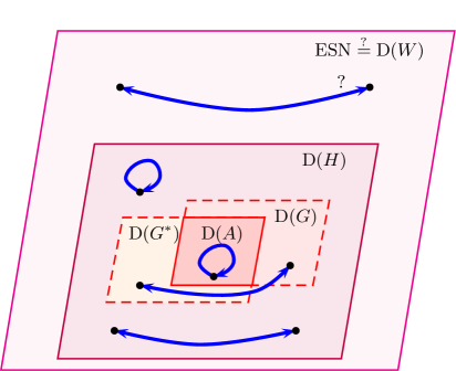
Figure 1: The duality landscape of quantum double models. We represent: Quantum doubles $\mathrm{D}(A)$ based on Abelian groups, including the toric code, all of which are self-dual; general group quantum double models $\mathrm{D}(G)$, related by duality to quantum double models $\mathrm{D}(G^{\ast})$ based on algebras of functions on groups, whose intersection with $\mathrm{D}(G)$ is $\mathrm{D}(A)$; these are all instances of quantum double models $\mathrm{D}(H)$ based on $C^{\ast}$-Hopf algebras, a larger class closed under duality, with cases of self-duality beyond groups [BMCA]. We conjecture that EM duality can be defined for all extended string-net models $\mathrm{ESN}$, and that these can be identified as quantum double models $\mathrm{D}(W)$ based on weak $C^{\ast}$-Hopf algebras. Arrows denote model identifications by EM duality.

At the level of SN models, dualities between two models are equivalences between two systems of bulk excitations. Mathematically, they correspond to braided equivalences of unitary modular tensor categories. As shown in [KK], they can be further identified with invertible (or transparent) domain walls. We will show in Section 9 that the EM duality between the electric and magnetic projections of an ESN model is canonically associated to a certain invertible domain wall. The corresponding domain wall at the level of ESN models is also briefly discussed.

In Section 10, we discuss a physical application of the EM duality in topology measurements in the form of pairs of dual tensor networks.

2 The toric code and self-duality

Let us begin by reviewing the well-known self-duality in the toric code [Ki], the quantum double model based on the group $\mathbb{Z}_{2}$. This is a model of qubits along the edges of a $2D$ lattice $\Lambda$, with a Hamiltonian of the form

$$\mathcal{H}=-\,\sum_{v}A_{v}-\,\sum_{p}B_{p}\;,$$ (1)

where $v$ runs over vertices and $p$ runs over plaquettes of $\Lambda$. Mutually commuting vertex and plaquette operators are projectors involving Pauli matrices:

$$A_{v}=\frac{1+\otimes_{i\in v}\sigma^{x}_{i}}{2}\;,\quad B_{p}=\frac{1+\otimes_{j\in p}\sigma^{z}_{j}}{2}\;,$$ (2)

with support on the edges around the corresponding vertex or plaquette. Ground states of the frustration-free Hamiltonian (1) minimise each term in the sum, that is, they satisfy all vertex and plaquette constraints $A_{v}|\psi\rangle=|\psi\rangle$, $B_{p}|\psi\rangle=|\psi\rangle$. Breakdown of any one such constraint means that the state is in an excited level, and can be interpreted as the presence of a localised excitation, or ‘particle’, sitting at the vertex or the plaquette whose constraint is broken; from the gauge theory interpretation, these are called electric and magnetic excitations, respectively.

Self-duality means that the global unitary

$$U_{\Lambda}=\otimes_{i\in\Lambda}U_{i}\;,\quad U_{i}=\frac{(\sigma^{x}+\sigma^{z})_{i}}{\sqrt{2}}\;,$$ (3)

built from Hadamard maps on each edge $i$, maps the toric code on $\Lambda$ to a toric code on the dual lattice $\Lambda^{\ast}$:

$$U_{\Lambda}\,A_{v}\,U_{\Lambda}^{\dagger}=\widetilde{B}_{v}\;,\quad U_{\Lambda}\,B_{p}\,U_{\Lambda}^{\dagger}=\widetilde{A}_{p}\;,$$ (4)

where now $\widetilde{B}_{v}$ corresponds to dual plaquette $v$, and $\widetilde{A}_{p}$ to dual vertex $p$ in $\Lambda^{\ast}$. The electric-magnetic nature of duality (4) comes from the interchange of vertices and plaquettes in going from the original to the dual lattice.

Hidden in the action of the global Hadamard map $U_{\Lambda}$ are $(a)$ the mapping from $\Lambda$ to $\Lambda^{\ast}$, with the corresponding reinterpretation of vertex and plaquette operators, and $(b)$ a mapping of the elements of the group $\mathbb{Z}_{2}$ to the functions from this group to the scalars. We obtain again a toric code on the dual lattice because, for an Abelian group, the space of functions has the same structure as the group algebra, which is the space of linear combinations of group elements. One can exploit this algebraic fact to extend the self-duality of the toric code to all quantum double models based on Abelian groups in a straightforward way: this is the $\mathrm{D}(A)$ region of Figure 1.

3 Quantum double models based on groups

Let us now define general quantum double models $\mathrm{D}(G)$ based on groups. Here, we start from a lattice with oriented edges, whose Hilbert spaces have an orthonormal basis $\{|g\rangle\}_{g\in G}$ labelled by elements of a finite group $G$. The Hamiltonian of the $\mathrm{D}(G)$ model is still of the form (1), but now the mutually commuting vertex and plaquette operators are the projectors defined in Figure 2.

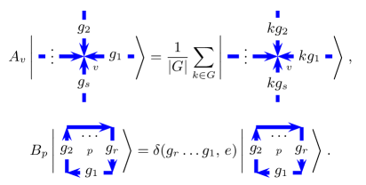
Figure 2: Projectors in the $\mathrm{D}(G)$ model. Vertex ($A_{v}$) and plaquette ($B_{p}$) projectors in the Hamiltonian of Kitaev’s $\mathrm{D}(G)$ model are defined by their action on a basis of the corresponding multi-edge Hilbert space. Oriented edges are labelled by group elements, denoting kets in the orthonormal computational basis $\{|g\rangle\}_{g\in G}$; change of orientation is implemented by applying the inversion map $g\mapsto g^{-1}$. The vertex operator projects onto gauge-invariant configurations, that is, symmetrises over simultaneous multiplication with group elements. The plaquette operator involves a Kronecker delta on the unit element $e\in G$ and projects onto trivial magnetic flux across $p$.

From the gauge theory point of view, edge degrees of freedom correspond to parallel transport operators taking values in the gauge group, vertex operators project onto gauge invariant configurations, and plaquette projectors minimise the Wilson action, i. e., they project onto configurations with trivial magnetic flux across the plaquette.

Excitations of the $\mathrm{D}(G)$ models are classified algebraically. Magnetic excitations, sitting on plaquettes, correspond to conjugacy classes of the gauge group; electric charges, sitting on vertices, are labelled by irreducible representations of $G$; and there are excitations, called dyons, living at the combination of a plaquette and a vertex and having both a magnetic part (a conjugacy class $C$ of $G$) and an electric part (an irreducible representation of the centraliser of $C$, which is a subgroup of $G$). In terms of more general algebraic structures, all these objects are just the irreducible representations of a quasitriangular Hopf algebra, Drinfel’d’s quantum double $\mathrm{D}(G)$ [Dr], and the distribution of topological charges over the lattice can be characterised by its reaction to operators representing this algebra, of which the vertex and plaquette projectors are examples.

The obvious parallelism of plaquettes and vertices in the Abelian case is lost if $G$ is non-Abelian. Upon switching to the dual lattice, we cannot reinterpret the operators $A_{v}$ and $B_{p}$ as, respectively, plaquette and vertex operators in a quantum double model based on a group, since the functions on a non-Abelian group no longer have the same structure as the group algebra itself. Hence, the extension of the EM duality to non-Abelian $\mathrm{D}(G)$ models is not possible within the class of quantum doubles based on groups. Yet dual models can be constructed which are quantum doubles based no longer on groups, but rather on algebras of functions; this is shown as the arrow between the regions $\mathrm{D}(G)$ and $\mathrm{D}(G^{\ast})$ in Figure 1.

To make sense of this, one has to widen the construction of quantum double lattice models beyond the group case. As we will show, the natural habitat for the EM duality of $\mathrm{D}(G)$ models is the class of quantum double models based on Hopf algebras [BMCA]; this is the region $\mathrm{D}(H)$ in Figure 1. This is the smallest class containing all the $\mathrm{D}(G)$ models that is closed under tensor products and EM duality. The duality, moreover, takes a remarkably simple form in the language of Hopf algebras.

4 The class of Hopf algebras

When studying quantum many-body systems, more general notions of symmetry emerge than those furnished by group theory. In particular, linear transformations acting on tensor products of vector spaces lead naturally to Hopf algebras. For a detailed account of these in our context we refer to [BMCA]. In the following we give an intuitive grasp of their structure, which is necessary to understand the $\mathrm{D}(H)$ lattice models.

We regard a Hopf algebra $H$ as a space of transformations on a many-body Hilbert space. First of all, the linear nature of the target is naturally extended to its transformations, so Hopf algebras are vector spaces. We must be able to compose transformations and to include the identity transformation, so $H$ has a multiplication of vectors, and a unit, making it into an algebra. Most importantly, we must have a rule to distribute the action of an element of $H$ into a tensor product of target spaces; this is the so-called comultiplication. Additionally $H$ has a trivial representation $\varepsilon$, called counit, making precise the notion of spaces invariant under the action of $H$. In the same way as for groups, the representation theory of Hopf algebras includes a notion of conjugate representation, implemented via an antipode mapping, which for groups is just the inversion $g\mapsto g^{-1}$.

To be able to construct Hilbert spaces we use finite-dimensional Hopf $C^{\ast}$-algebras, where an inner product can be defined. In addition, they come equipped with a canonical, normalised, highly symmetric element, the Haar integral $h\in H$, invariant under multiplication in the sense $a\cdot h=\varepsilon(a)\,h$ for all elements $a$ of $H$. This canonical element is crucial for the construction of the lattice model and its ground states.

A graphical language which is particularly advantageous for the treatment of Hopf algebras is outlined with reference to the first row of Figure 3. Each diagram in the first row represents one of the structure maps of a Hopf algebra as introduced above: multiplication, unit, comultiplication, counit, and antipode, all viewed as linear mappings from a vector space at the bottom of the diagram to a vector space at the top of the diagram. Tensor factors of these vector spaces are represented by juxtaposition.

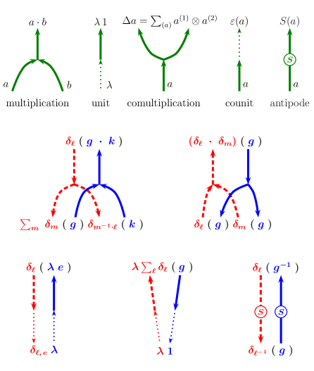
Figure 3: Structure and dualities in Hopf algebras. The first row represents the structure maps of a Hopf algebra $H$. The second and third rows illustrate the algebraic duality within the class of Hopf algebras, taking as examples a group algebra $H=\mathbb{C}G$ and its dual $H^{\ast}$, whose structure is defined implicitly in the figure.

The root of the EM duality to be unveiled in the following is an algebraic fact: The class of finite-dimensional Hopf $C^{\ast}$-algebras is closed under dualisation. That is, given a finite-dimensional $C^{\ast}$-Hopf algebra $H$, its dual space $H^{\ast}$ (the functions from $H$ to the scalars) is again a finite-dimensional $C^{\ast}$-Hopf algebra, whose structure is, moreover, determined by the structure of $H$. This closure property is shared by the class of Abelian group algebras, which are all self-dual, but not by the whole class of group algebras. The landscape of Figure 1 reflects these statements in the world of lattice models.

With reference to the second and third rows of Figure 3, we use the case where the Hopf algebra is a group algebra, $H=\mathbb{C}G$ to illustrate the algebraic duality in the class of Hopf algebras. For each diagram, the upper expression is equal to the lower expression; the structure maps of $H$ and $H^{\ast}$ are represented by solid and dashed lines, respectively, according to the conventions of the first row. Hence, the comultiplication in $H^{\ast}$ is determined by the multiplication in $H$, the multiplication in $H^{\ast}$ is determined by the comultiplication in $H$, the counit in $H^{\ast}$ is determined by the unit in $H$, the unit in $H^{\ast}$ is determined by the counit in $H$, and the antipode in $H^{\ast}$ is determined by the antipode in $H$; this duality holds for general finite-dimensional Hopf algebras. We use the form of the structure maps in the basis $\{g;\,g\in G\}$ of the group algebra, and the basis $\{\delta_{\ell};\,\ell\in G\}$ of its dual, where $\delta_{\ell}\colon g\mapsto\delta_{\ell,\,g}$ are Kronecker delta functions. As for the extra structure needed to define our lattice models, the $C^{\ast}$-algebra structures of $H$ and $H^{\ast}$ are defined by declaring $\{g\}$ to be an orthonormal basis, and $\{\delta_{\ell}\}$ to be orthonormal up to a factor, $(\delta_{\ell},\,\delta_{m})=|G|^{-1}\,\delta_{\ell,\,m}$. The Haar integrals $h$ and $\phi$ in the group algebra and its dual are defined in equation (6) below.

5 The $\mathrm{D}(H)$ lattice models

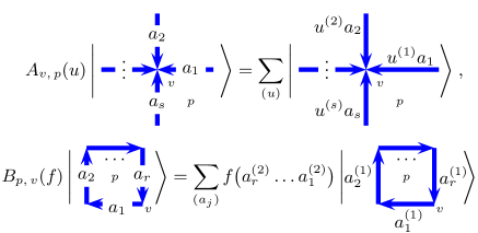
Figure 4: The core of $\mathrm{D}(H)$ models. Topological models based on Hopf algebras are defined via these vertex and plaquette representations of elements $u$ of Hopf algebra $H$ and elements $f$ of the dual $H^{\ast}$.

Quantum double models based on Hopf algebras, $\mathrm{D}(H)$ models for short, are a class of topological models, defined on $2D$ lattices whose local Hilbert space along oriented edges is a finite-dimensional $C^{\ast}$-Hopf algebra $H$. Figure 4 defines a set of operators on this lattice which depend on elements $u\in H$ and $f\in H^{\ast}$. Oriented edges carry, in general, elements of the finite-dimensional $C^{\ast}$-Hopf algebra $H$. Orientation can be reversed by using the antipode map $S$. The sums in the formulas of Figure 4 denote the appropriate comultiplication or splitting of algebra elements $u$ into several tensor factors $\sum u^{(1)}\otimes u^{(2)}\otimes\ldots\otimes u^{(s)}$. Vertex operators $A_{v,\,p}$ now depend also on a plaquette $p$ marking the beginning of a loop around the vertex $v$, and correspondingly for the plaquettes. These operators probe the algebraic structure of the models: Given overlapping vertex $v$ and plaquette $p$, the corresponding vertex operator $A_{v,\,p}(u)$ and the plaquette operator $B_{p,\,v}(f)$ interact nontrivially with each other, building representations of Drinfel’d’s quantum double algebra $\mathrm{D}(H)$ [Dr]. The irreducible representations of $\mathrm{D}(H)$ classify the superselection sectors, and thus the anyonic excitations, of the quantum double lattice model [Ki].

When elements $u$ and $f$ in Figure 4 are taken as the canonical Haar integrals $h\in H$ and $\phi\in H^{\ast}$, respectively, the resulting operators

$$A_{v}=A_{v,\,p}(h)\;,\quad B_{p}=B_{p,\,v}(\phi)$$ (5)

are mutually commuting projectors defining via (1) the Hamiltonian of the $\mathrm{D}(H)$ model [BMCA]. The Hamiltonian is thus entirely constructed from the canonical elements $h$, $\phi$ and the algebraic structure of $H$.

Kitaev’s models constitute a subclass of $\mathrm{D}(H)$ models, recovered when $H$ is the group algebra of a finite group $G$. Both this algebra $\mathbb{C}G$ and its dual $G^{\ast}$ have particularly simple $C^{\ast}$-Hopf algebra structures, summarised in the second and third rows of Figure 3. In particular, their Haar integrals read

$$h=\frac{1}{|G|}\,\sum_{g\in G}g\in\mathbb{C}G\;,\quad\phi=\delta_{e}\in G^{\ast}\;.$$ (6)

Taking into account this equation, operators in Figure 2, defining the Hamiltonian of the $\mathrm{D}(G)$ model, can be checked to coincide with the general expression (5).

6 Electric-magnetic duality

We now define EM duality for general $\mathrm{D}(H)$ models. Consider the following unitary map $U$ from $H$ to its dual $H^{\ast}$:

$$a\stackrel{{\scriptstyle U}}{{\longmapsto}}f_{a}\;,\quad f_{a}(b)=\sqrt{\dim H}\,\phi(a\cdot b)\;,$$ (7)

where the function $f_{a}$ is constructed via the dual Haar integral $\phi\in H^{\ast}$ (for instance, for groups, $f_{g}=\sqrt{|G|}\,\delta_{g^{-1}}$). We associate this mapping with the transformation of $\Lambda$ into its dual lattice $\Lambda^{\ast}$ as shown in Figure 5. In this figure, the solid edge is in $\Lambda$, while the dashed edge is its dual in $\Lambda^{\ast}$. The orientation of the dual edge is chosen by convention so that it points to the left of the direct edge. The degree of freedom $a\in H$ in the Hilbert space $H$ of the edge in $\Lambda$ becomes a degree of freedom $f_{a}$ of the Hilbert space $H^{\ast}$ of the dual edge. When applied simultaneously on all edges of $\Lambda$, this mapping implements EM duality.

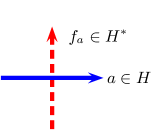
Figure 5: Going over to the dual lattice. The mapping $U\colon H\rightarrow H^{\ast}$ is here associated with a lattice dualisation $\Lambda\rightarrow\Lambda^{\ast}$.

The vertex and plaquette representations in Figure 4, which in particular determine the Hamiltonian of the $\mathrm{D}(H)$ model on $\Lambda$, are mapped by the global operation $U_{\Lambda}=\bigotimes_{i\in\Lambda}U_{i}$ into precisely the representations associated with the $\mathrm{D}(H^{\ast})$ model on the dual lattice $\Lambda^{\ast}$:

$$U_{\Lambda}\,B_{p,\,v}(f)\,U_{\Lambda}^{\dagger}={\widetilde{A}}_{p,\,v}(f)\;,\quad U_{\Lambda}\,A_{v,\,p}(u)\,U_{\Lambda}^{\dagger}={\widetilde{B}}_{v,\,p}(u)\;,$$ (8)

where $u\in H$ and $f\in H^{\ast}$. Here $p$ is a plaquette of $\Lambda$ and a vertex of $\Lambda^{\ast}$; $v$ is a vertex of $\Lambda$ and a plaquette of $\Lambda^{\ast}$. Expression (8) generalises equation (4), singling out $U_{\Lambda}$ as the EM duality mapping.

Thus, $U_{\Lambda}$ identifies the $\mathrm{D}(H)$ model on $\Lambda$ with the $\mathrm{D}(H^{\ast})$ model on $\Lambda^{\ast}$, as it unitarily transforms the Hilbert spaces and Hamiltonian of the former into those of the latter. We write this symbolically as $[\mathrm{D}(H)]_{\Lambda}=[\mathrm{D}(H^{\ast})]_{\Lambda^{\ast}}$.

But EM duality is deeper than a mere identification of energy levels. The Hamiltonian involves just the operators $A_{v}(h)$ and $B_{p}(\phi)$, but, according to (8), $U_{\Lambda}$ induces a transformation of all operators of Figure 4 that respects their algebra structure, and relates the anyonic excitations of both models.

7 From quantum doubles to extended string-nets

In [BA] the $\mathrm{D}(G)$ model was identified, via a Fourier transformation, with an extended string-net model on the same lattice. In particular, the edge degrees of freedom can be spanned by a Fourier basis

$$|\mu ab\rangle=\sqrt{\frac{\dim\mu}{|G|}}\sum_{g\in G}\,\,D^{\mu}(g)_{ab}|g\rangle,$$ (9)

where $\mu$ runs over the irreducible representations (irreps) of $G$ and $D^{\mu}$ is a fixed matrix realization of the irreducible representation $\mu$. Using this new basis, $A_{v}$ and $B_{p}$ operators in the Hamiltonian can both be expressed in terms of certain projectors [BA, Eq.(11)(17)] as follows:

$$A_{v}|\{\mu_{i}a_{i}b_{i}\}\rangle_{v}=\sum_{c_{1},\cdots,c_{r}}W_{\{c_{i}\},\{b_{i}\}}^{\{\mu_{i}\}}|\{\mu_{i}a_{i}b_{i}\}\rangle_{v}$$ (10)

where

$$W_{\{c_{i}\},\{b_{i}\}}^{\{\mu_{i}\}}=\frac{1}{|G|}\sum_{l\in G}\prod_{i}D^{\mu_{i}}(l)_{c_{i}b_{i}}$$

is the projector onto the trivial isotopic subspace of $\otimes_{i}\mu_{i}$, and

$$B_{p}\coloneqq\sum_{\nu}\frac{\dim\nu}{|G|}B_{p}(\nu)$$ (11)

with $B_{p}(\nu)$ acting on a hexagon-shaped plaquette as follows:

$$\langle\{\mu_{j}^{\prime}a_{j}^{\prime}b_{j}^{\prime}\}|B_{p}(\nu)|\{\mu_{j}a_{j}b_{j}\}\rangle=\prod_{i=1}^{6}\sqrt{\dim\mu_{i}\dim\mu_{i}^{\prime}}\sum_{c_{1},\cdots,c_{6}}\prod_{i=1}^{6}W_{a_{i}a_{i}^{\prime}c_{i},b_{i}b_{i}^{\prime}c_{i+1}}^{\mu_{i}\mu_{i}^{\prime}\nu}$$ (12)

where the index $i$ is cyclic, i.e. $i+1=1$ when $i=6$.

The representation theory of finite-dimensional $C^{\ast}$-Hopf algebras is essentially identical to that of finite groups, the only real difference being that the fusion of representations need not be commutative. Therefore the construction of [BA] generalizes to any $\mathrm{D}(H)$ model. That is, if $H$ has matrix irreps $D^{\mu}$ associated to irrep $\mu$, we define a Fourier basis in $H$ containing the following algebra elements:

$$|\mu ab\rangle=\sqrt{\frac{\dim\mu}{\dim H}}\,\sum_{(h)}D^{\mu}(h^{(1)})_{ab}\,h^{(2)}\;,$$ (13)

where $a,\,b=1,\,\ldots,\,\dim\mu$ are matrix indices for irrep $D^{\mu}$. This is an orthonormal basis for the Hilbert spaces at each edge. The analysis of [BA] carries through intact to show that the $[\mathrm{D}(H)]_{\Lambda}$ model can be written as an extended string-net model $[\mathrm{ESN}_{(\mathcal{C},\omega)}]_{\Lambda}$, where the meaning of $(\mathcal{C},\omega)$ will be explained later, with edge degrees of freedom labeled by triplets $|\mu ab\rangle$.

Readers might wonder why we give the $[\mathrm{D}(H)]_{\Lambda}$ model the new name “extended string-net model $[\mathrm{ESN}_{(\mathcal{C},\omega)}]_{\Lambda}$”. The reason is that the above construction for the $[\mathrm{D}(H)]_{\Lambda}$ model can be reformulated completely in terms of tensor categorical notions, i.e. a pair $(\mathcal{C},\omega)$ (explained later), without referring to groups or Hopf algebras at all. This reformulation, which will be given explicitly below, is important and deserves a new name because we believe that the tensor-categorical structures should be viewed as more fundamental than groups or Hopf algebras, and the latter notions should be viewed as symmetries emerging from the former notions. Such a point of view was expressed earlier in [LW] and will be made more precise in this article. Mathematically, this reformulation is possible due to the so-called Tannaka-Krein duality [U] which explains the equivalence between the notion of a Hopf algebra and that of a tensor category $\mathcal{C}$ equipped with a fiber functor $\omega$.

In the rest of this section we outline the definition of ESN models purely from tensor-categorical structures. The developments in the following sections will be presented in terms of the quantum double and/or the tensor-categorical formulation where appropriate.

We will start from a unitary finite fusion category $\mathcal{C}$ with simple objects $\mu,\nu,\lambda,\ldots\in I$, where $I$ is a finite set, and a simple unit $1_{\mathcal{C}}\in I$. Associating auxiliary matrix indices with each simple object in $\mathcal{C}$ amounts to assigning a vector space $\omega(\mu)$ to each simple object $\mu\in I$. In the quantum double model picture, $\mu$ is the label for an irreducible representation of a finite group or a Hopf algebra, and $\omega(\mu)$ is nothing but the representation space associated with $\mu$. It is easy to generalize this assignment to all objects in $\mathcal{C}$ by requiring $\mu\oplus\nu\mapsto\omega(\mu)\oplus\omega(\nu)$ for $\mu,\nu\in I$ so that we obtain a functor $\omega\colon\mathcal{C}\to\mathcal{H}\mathrm{ilb}$, where $\mathcal{H}\mathrm{ilb}$ is the category of finite dimensional Hilbert spaces. The assignment $\omega(\mu)$ cannot be arbitrary. The consistency condition needed for the construction of our lattice models is that the functor $\omega\colon\mathcal{C}\to\mathcal{H}\mathrm{ilb}$ is a monoidal functor. In particular, it means that there are isomorphisms

$$\phi_{2}\colon\omega(\mu\otimes\nu)\xrightarrow{\simeq}\omega(\mu)\otimes\omega(\nu)$$ (14)

and $\phi_{0}\colon\omega(1_{\mathcal{C}})\xrightarrow{\simeq}\mathbb{C}$ satisfying certain coherence conditions. Such a functor $\omega$ is called a fiber functor of $\mathcal{C}$.

We would like to build a Hamiltonian model on a trivalent lattice with oriented edges. Note that the restriction to trivalent lattices (instead of more general planar lattices) is merely a matter of convenience. We associate to each oriented internal edge $e$ a Hilbert space

$$\mathcal{H}_{e}=H_{(\mathcal{C},\omega)}=\oplus_{\mu\in I}\,\,\omega(\mu)\otimes\omega(\mu)^{\ast},$$ (15)

where $\omega(\mu)^{\ast}$ is the dual vector space of $\omega(\mu)$. The total Hilbert space is just $\mathcal{H}=\otimes_{e}\mathcal{H}_{e}$.

The Hamiltonian is still defined as:

$$H=-\sum_{v}A_{v}-\sum_{p}B_{p},$$ (16)

where $v$ labels the trivalent vertices and $p$ labels the plaquettes. The operator $A_{v}$ for each trivalent vertex $v$ (with all edges pointing towards $v$) is a linear map: $\otimes_{i=1}^{3}\omega(\mu_{i})^{\ast}\otimes\omega(\mu_{i})\rightarrow\otimes_{i=1}^{3}\omega(\mu_{i})^{\ast}\otimes\omega(\mu_{i})$ defined by:

$$A_{v}\coloneqq P_{\omega(\mu_{1})\omega(\mu_{2})\omega(\mu_{3})}\otimes\mathrm{id}_{\omega(\mu_{1})^{\ast}}\otimes\mathrm{id}_{\omega(\mu_{2})^{\ast}}\otimes\mathrm{id}_{\omega(\mu_{3})^{\ast}},$$ (17)

where $P_{\omega(\mu_{1})\omega(\mu_{2})\omega(\mu_{3})}\colon\otimes_{i=1}^{3}\omega(\mu_{i})\rightarrow\otimes_{i=1}^{3}\omega(\mu_{i})$ is intuitively the projection onto the vacuum channel. However, we do not know if $\mathcal{C}$ is the category of representations of any group or Hopf algebra a priori. We must therefore define $P_{\omega(\mu_{1})\omega(\mu_{2})\omega(\mu_{3})}$ independently in terms of the data in $\mathcal{C}$ and the fiber functor $\omega$. Note that the fusion rule in $\mathcal{C}$ gives a canonical projector morphism $P_{\mu_{1}\mu_{2}\mu_{3}}\colon\mu_{1}\otimes\mu_{2}\otimes\mu_{3}\to\oplus 1_{\mathcal{C}}$ in $\mathcal{C}$ that maps $\mu_{1}\otimes\mu_{2}\otimes\mu_{3}$ to the subobject consisting of only a direct sum of copies of the unit object $1_{\mathcal{C}}$. Since $\omega$ is monoidal, using (14), we obtain a canonical isomorphism

$$\phi_{3}\colon\omega(\mu_{1})\otimes\omega(\mu_{2})\otimes\omega(\mu_{3})\xrightarrow{\cong}\omega(\mu_{1}\otimes\mu_{2}\otimes\mu_{3}).$$ (18)

Then we define $P_{\omega(\mu_{1})\omega(\mu_{2})\omega(\mu_{3})}\coloneqq\phi_{3}^{-1}\circ\omega(P_{\mu_{1}\mu_{2}\mu_{3}})\circ\phi_{3}$. It is clear that $P_{\omega(\mu_{1})\omega(\mu_{2})\omega(\mu_{3})}$ so defined is a projector.

The operator $B_{p}$ for each plaquette $p$ (taken, for convenience only, as a hexagon) is a map:

$$B_{p}\colon\otimes_{i=1}^{6}(\oplus_{\lambda_{i}}\omega(\lambda_{i})^{\ast}\otimes\omega(\lambda_{i}))\rightarrow\otimes_{i=1}^{6}(\oplus_{\mu_{i}}\omega(\mu_{i})^{\ast}\otimes\omega(\mu_{i}))$$

which can be viewed as an element in the space

$$\oplus_{\{\mu_{i}\}}\oplus_{\{\lambda_{i}\}}\otimes_{i=1}^{6}(\omega(\mu_{i})^{\ast}\otimes\omega(\mu_{i})\otimes\omega(\lambda_{i}^{\ast})^{\ast}\otimes\omega(\lambda_{i}^{\ast}))$$ (19)

where we have used $\omega(\lambda^{\ast})\cong\omega(\lambda)^{\ast}$ because $\omega$ is monoidal. We define this element $B_{p}$ to be

$$B_{p}=\sum_{\nu\in I}\frac{\dim\omega(\nu)}{\dim\mathcal{H}_{e}}\,\,B_{p}(\nu),$$ (20)

where $B_{p}(\nu)$ is again an element in the space of (19). We define $B_{p}(\nu)$ in the following way. First we have the element

$$\oplus_{\{\mu_{i}\}}\oplus_{\{\lambda_{i}\}}\otimes_{i=1}^{6}\sqrt{\dim\mu_{i}\dim\lambda_{i}}\,P_{\omega(\mu_{i})\omega(\lambda_{i}^{\ast})\omega(\nu_{i})},$$

where all $\nu_{i}=\nu$, in the space

$$\oplus_{\{\mu_{i}\}}\oplus_{\{\lambda_{i}\}}\otimes_{i=1}^{6}(\omega(\mu_{i})^{\ast}\otimes\omega(\mu_{i})\otimes\omega(\lambda_{i}^{\ast})^{\ast}\otimes\omega(\lambda_{i}^{\ast})\otimes\omega(\nu_{i})\otimes\omega(\nu_{i})^{\ast}).$$ (21)

Using the evaluation map $\mathrm{ev}_{i}\colon\omega(\nu_{i})^{\ast}\otimes\omega(\nu_{i+1})\rightarrow\mathbb{C},i=1,\dots,6$ where $\nu_{7}=\nu_{1}$, we obtain a map $\otimes_{i=1}^{6}\mathrm{ev}_{i}$ from the space (21) to the space (19). Then we define

$$B_{p}(\nu)\coloneqq\otimes_{i=1}^{6}\mathrm{ev}_{i}(\oplus_{\{\mu_{i}\}}\oplus_{\{\lambda_{i}\}}(\otimes_{i=1}^{6}\sqrt{\dim\mu_{i}\dim\lambda_{i}}\,P_{\omega(\mu_{i})\omega(\lambda_{i}^{\ast})\omega(\nu_{i})})).$$ (22)

If $\mathcal{C}=\mathrm{Rep}_{H}$ for some $C^{\ast}$-Hopf algebra $H$, then we simply take $\omega$ to be the forgetful functor $F\colon\mathrm{Rep}_{H}\to\mathcal{H}\mathrm{ilb}$. Then the Hilbert space $H_{(\mathcal{C},\omega)}$ (recall Eq. (15)) is isomorphic to the underlying Hilbert space of the $C^{\ast}$-Hopf algebra $H$. Moreover, it is easy to check that the definition of $A_{v}$ and $B_{p}$ (Eq. (17), (20), (22)) coincides exactly with that of $A_{v}$ and $B_{p}$ (see for example Eq. (10), (11), (12) in $\mathrm{D}(G)$ cases) in $\mathrm{D}(H)$ models. Therefore, we have

$$[\mathrm{D}(H)]_{\Lambda}=[\mathrm{ESN}_{(\mathrm{Rep}_{H},F)}]_{\Lambda}.$$

Conversely, for any unitary finite fusion category $\mathcal{C}$ admitting a fiber functor $\omega$, the Hilbert space $H_{(\mathcal{C},\omega)}$ is automatically equipped with the structure of a semisimple $C^{\ast}$-Hopf algebra such that $\mathcal{C}\simeq\mathrm{Rep}_{H_{(\mathcal{C},\omega)}}$. This result is nothing but the statement of the so-called Tannaka-Krein duality [U].

The EM-duality for ESN models can be defined in terms of tensor-categorical notions as well. On the one hand, given a pair $(\mathcal{C},\omega)$, the category $\mathcal{H}\mathrm{ilb}$ is automatically a $\mathcal{C}$-module. Then we can define the dual tensor category

$$\mathcal{C}^{\ast}\coloneqq\mathrm{Fun}_{\mathcal{C}}(\mathcal{H}\mathrm{ilb},\mathcal{H}\mathrm{ilb})^{\otimes_{\mathrm{op}}}$$

by the category of $\mathcal{C}$-module functors from $\mathcal{H}\mathrm{ilb}$ to $\mathcal{H}\mathrm{ilb}$ with tensor product defined by the opposite composition of functors. The dual tensor category $\mathcal{C}^{\ast}$ is again a unitary finite fusion category. Moreover, $\mathcal{H}\mathrm{ilb}$ is naturally equipped with a $\mathcal{C}^{\ast}$-module structure, which further gives rise to a fiber functor [Os] $\omega^{\ast}\colon\mathcal{C}^{\ast}\to\mathcal{H}\mathrm{ilb}$. More explicitly, $\omega^{\ast}$ can be defined by $\omega^{\ast}\colon F\mapsto F(\mathbb{C})$ for $F\in\mathcal{C}^{\ast}$, where $\mathbb{C}$ is the tensor unit of $\mathcal{H}\mathrm{ilb}$. By the proof of Theorem 5 in [Os], it is easy to conclude that $H_{(\mathcal{C}^{\ast},\omega^{\ast})}\simeq H_{(\mathcal{C},\omega)}^{\ast}$ as Hopf algebras. In other words, we have

$$[\mathrm{ESN}_{(\mathcal{C},\omega)}]_{\Lambda}=[\mathrm{D}(H_{(\mathcal{C},\omega)})]_{\Lambda}\xleftrightarrow{\mbox{EM duality}}[\mathrm{D}(H_{(\mathcal{C},\omega)}^{\ast})]_{\Lambda^{\ast}}=[\mathrm{ESN}_{(\mathcal{C}^{\ast},\omega^{\ast})}]_{\Lambda^{\ast}}.$$

In tensor-categorical language, the EM duality is a duality between $(\mathcal{C},\omega)$ and $(\mathcal{C}^{\ast},\omega^{\ast})$. Indeed, it is easy to show that $(\mathcal{C}^{\ast\ast},\omega^{\ast\ast})=(\mathcal{C},\omega)$. This categorical duality is related to the Morita equivalence between $\mathcal{C}$ and its dual $\mathcal{C}^{\ast}$. We will explain this point in Section 9 where the EM duality is studied from the perspective of domain wall.

8 From extended string-net models to string-net models

We now make the connection with string-net models. String-net models were introduced by Levin and Wen in [LW] and further developed and enriched by boundaries and defects of all codimensions in [KK].

The local Hilbert spaces of SN models, solely determined by the data of a unitary tensor category $\mathcal{C}$, are different from those of ESN models in general. However, the ground levels of SN models and their extended versions are identical. They describe the same topological phases. Given an $[\mathrm{ESN}_{(\mathcal{C},\omega)}]_{\Lambda}$ model (or equivalently a $[\mathrm{D}(H_{(\mathcal{C},\omega)})]_{\Lambda}$ model), one can project out the additional degrees of freedom controlled by the fiber functor $\omega\colon\mathcal{C}\to\mathcal{H}\mathrm{ilb}$, in a manner entirely analogous to the construction in [BA], to obtain a SN model defined by the unitary tensor category $\mathcal{C}$. This resulting SN model is called the magnetic projection of the original ESN model on $\Lambda$, and will be denoted as $[\mathrm{SN}_{\mathcal{C}}^{\mathrm{mag}}]_{\Lambda}$.

The same construction can be applied to the $[\mathrm{ESN}_{(\mathcal{C}^{\ast},\omega^{\ast})}]_{\Lambda^{\ast}}$ model (or equivalently the $[\mathrm{D}(H_{(\mathcal{C},\omega)}^{\ast})]_{\Lambda^{\ast}}$ model). Its magnetic projection is a string-net model $[\mathrm{SN}_{\mathcal{C}^{\ast}}^{\mathrm{mag}}]_{\Lambda^{\ast}}$. We will call $[\mathrm{SN}_{\mathcal{C}^{\ast}}^{\mathrm{mag}}]_{\Lambda^{\ast}}$ the electric projection of $[\mathrm{ESN}_{(\mathcal{C},\omega)}]_{\Lambda}$, i.e. $[\mathrm{SN}_{\mathcal{C}}^{\mathrm{el}}]_{\Lambda}\coloneqq[\mathrm{SN}_{\mathcal{C}^{\ast}}^{\mathrm{mag}}]_{\Lambda^{\ast}}$.

The EM duality between $[\mathrm{ESN}_{(\mathcal{C},\omega)}]_{\Lambda}$ and $[\mathrm{ESN}_{(\mathcal{C}^{\ast},\omega^{\ast})}]_{\Lambda^{\ast}}$ induces a duality between $[\mathrm{SN}_{\mathcal{C}}^{\mathrm{mag}}]_{\Lambda}$ and $[\mathrm{SN}_{\mathcal{C}^{\ast}}^{\mathrm{mag}}]_{\Lambda^{\ast}}$, which describe the same topological phase. This net of correspondences and dualities is illustrated in Figure 6.

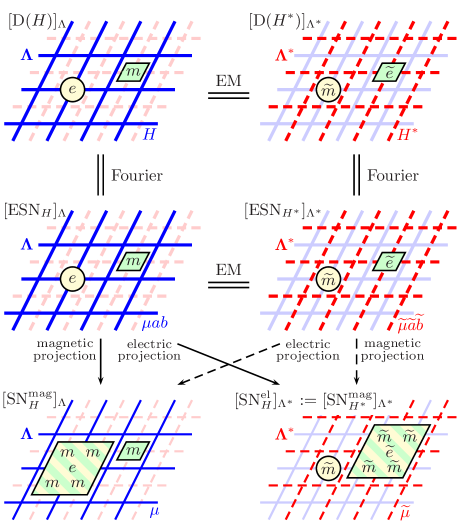
Figure 6: From quantum doubles to string-nets. Quantum double models and string-net models are interconnected by EM duality, the Fourier mapping, and a projection to SN degrees of freedom as illustrated herein and discussed in detail in the text.

In this figure, the direct lattice is drawn solid, the dual lattice dashed. The first layer represents a quantum double model in its two EM-dual formulations on the direct and dual lattices $\Lambda$ and $\Lambda^{\ast}$. Via a Fourier mapping we write the quantum doubles as extended string-net models, depicted in the second layer, which are entirely equivalent. The degrees of freedom of the ESN model on $\Lambda$ are labelled by irreducible representations $\mu$ of $H$ and auxiliary matrix indices $a$, $b$; for the dual model on $\Lambda^{\ast}$ the labels are irreducible representations $\widetilde{\mu}$ of $H^{\ast}$, and auxiliary matrix indices $\widetilde{a}$, $\widetilde{b}$. These models support excitations both at vertices (electric) and at plaquettes (magnetic), which we represent by blobs and lozenges. An electric excitation $e$ becomes a magnetic excitation $\widetilde{m}$ in the dual, and vice versa. The third layer in Figure 6 represents the string-net models obtained, respectively, by projecting to degrees of freedom $\mu$ on the direct lattice, or to $\widetilde{\mu}$ on the dual lattice; these we refer to as magnetic and electric projections of the ESNs, respectively. Excitations in SN models are less symmetric than in the ESN: for instance, violation of a vertex constraint implies the violation of all surrounding plaquette constraints (see [BA]). This is due to the fact that the local Hilbert spaces of a SN model is too small to support a well-defined splitting of electric and magnetic excitations.

For instance, in [BA] the magnetic SN projection of the $\mathrm{D}(G)$ model was analysed. Its electric SN projection, on the other hand, has the same local degrees of freedom as the $\mathrm{D}(G)$ model, since group elements are the (one-dimensional) irreps of the dual of the group algebra. This connection of SN and $\mathrm{D}(G)$ models had been recognised long ago by Héctor Bombín [B].

9 EM duality and domain walls

A duality-defect correspondence was obtained in [KK]. In particular, it was shown that invertible dualities between two bulk SN models based on the unitary tensor categories $\mathcal{C}$ and $\mathcal{D}$ are in one-to-one correspondence with the invertible domain walls between these two SN models. Therefore, the EM duality between $[\mathrm{SN}_{\mathcal{C}}^{\mathrm{mag}}]_{\Lambda}$ and $[\mathrm{SN}_{\mathcal{C}^{\ast}}^{\mathrm{mag}}]_{\Lambda^{\ast}}$ defined (for a given fiber functor) in Section 8 must correspond to an invertible domain wall. This domain wall, depicted in Fig. 7, is nothing but the category $\mathcal{H}\mathrm{ilb}$, which is viewed as an invertible $\mathcal{C}$-$\mathcal{C}^{\ast}$-bimodule. Moreover, the category $\mathcal{H}\mathrm{ilb}$ defines a Morita equivalence between $\mathcal{C}$ and $\mathcal{C}^{\ast}$, and provides a braided equivalence (defined below by Eq. (23) when $\mathcal{M}=\mathcal{H}\mathrm{ilb}$) from the bulk excitations $Z(\mathcal{C})$ to the bulk excitations $Z(\mathcal{C}^{\ast})$. This braided equivalence describes exactly how a bulk excitation in a $\mathcal{C}$-lattice tunnels through the domain wall into a $\mathcal{C}^{\ast}$-lattice [KK].

Figure 7: A neighborhood of a defect line between a $\mathcal{C}$-lattice and a $\mathcal{C}^{\ast}$-lattice, where $\mu_{i}\in\mathcal{C}$ and $\nu_{i}^{\prime}\in\mathcal{C}^{\ast}$. There is no edge label on the domain wall because there is only one simple object $\mathbb{C}$ in $\mathcal{H}\mathrm{ilb}$.

Although we can define the EM duality between two SN models obtained from the magnetic and electric projections of a given ESN model, there is no way to define EM duality for general SN models because (i) a fiber functor $\mathcal{C}\to\mathcal{H}\mathrm{ilb}$ does not exist in general (and so a parent ESN model as introduced above does not exist, either), and (ii) even if such a fiber functor does exist it is not unique in general. In other words, each fiber functor is as canonical as any other and does not deserve to be called “the” EM duality.

It is, however, possible to associate to every SN model based on a unitary tensor category $\mathcal{C}$ a family of dualities parametrized by indecomposable semisimple $\mathcal{C}$-modules. Indeed, given such a $\mathcal{C}$-module $\mathcal{M}$, we can define the dual tensor category $\mathcal{C}_{\mathcal{M}}^{\ast}\coloneqq\mathrm{Fun}_{\mathcal{C}}(\mathcal{M},\mathcal{M})^{\otimes_{\mathrm{op}}}$ by the category of $\mathcal{C}$-module functors from $\mathcal{M}$ to $\mathcal{M}$ with tensor product defined by the opposite composition of functors. Then there is a duality between the SN model based on $\mathcal{C}$ and that based on $\mathcal{C}_{\mathcal{M}}^{\ast}$. This duality $\alpha_{\mathcal{M}}$ is precisely determined by the domain wall (or the defect line) associated to $\mathcal{M}$ via the duality-defect correspondence [KK]. More precisely, the duality $\alpha_{\mathcal{M}}$, as an invertible braided monoidal functor $\alpha_{\mathcal{M}}\colon Z(\mathcal{C})\to Z(\mathcal{C}_{\mathcal{M}}^{\ast})$ from the bulk excitations $Z(\mathcal{C})$ of a $\mathcal{C}$-lattice to the bulk excitations $Z(\mathcal{C}_{\mathcal{M}}^{\ast})$ of a $\mathcal{C}_{\mathcal{M}}^{\ast}$-lattice, is defined by:

$$Z(\mathcal{C})=\mathrm{Fun}_{\mathcal{C}|\mathcal{C}}(\mathcal{C},\mathcal{C}) \to\mathrm{Fun}_{\mathcal{C}|\mathcal{C}}(\mathcal{M}^{\mathrm{op}}\boxtimes_{\mathcal{C}}\mathcal{C}\boxtimes_{\mathcal{C}}\mathcal{M},\mathcal{M}^{\mathrm{op}}\boxtimes_{\mathcal{C}}\mathcal{C}\boxtimes_{\mathcal{C}}\mathcal{M})\simeq Z(\mathcal{C}_{\mathcal{M}}^{\ast})$$

$$\mathcal{F} \mapsto\mathrm{id}_{\mathcal{M}^{\mathrm{op}}}\boxtimes_{\mathcal{C}}\mathcal{F}\boxtimes_{\mathcal{C}}\mathrm{id}_{\mathcal{M}}.$$ (23)

If $\mathcal{C}$ is equipped with a fiber functor $\omega\colon\mathcal{C}\to\mathcal{H}\mathrm{ilb}$, then the category $\mathcal{H}\mathrm{ilb}$ is automatically a $\mathcal{C}$-module. Then the functor $\alpha_{\mathcal{M}}$ for $\mathcal{M}=\mathcal{H}\mathrm{ilb}$ defines the EM duality between the bulk excitations in $[\mathrm{SN}_{\mathcal{C}}^{\mathrm{mag}}]_{\Lambda}$ and those in $[\mathrm{SN}_{\mathcal{C}^{\ast}}^{\mathrm{mag}}]_{\Lambda^{\ast}}$.

We have shown that EM duality can be realized by an invertible domain wall (or a defect line) at the level of SN models. We would like to mention that it is also possible to associate EM duality to an invertible domain wall at the level of ESN models. The theory of ESN models enriched by boundaries and defects demands many new mathematical notions and tools, and will be developed elsewhere [Ko2]. We will provide a quick glance here into this rich theory so that we will be able to say something about the EM duality.

The boundary-defect theory of ESN models relies on a generalization of the representation theory of a tensor category $\mathcal{C}$ to that of a pair $(\mathcal{C},\omega_{\mathcal{C}})$ where $\omega_{\mathcal{C}}$ is a fiber functor. In particular, a $(\mathcal{C},\omega_{\mathcal{C}})$-module is a pair $(\mathcal{M},\omega_{\mathcal{M}})$ where $\mathcal{M}$ is a $\mathcal{C}$-module and $\omega_{\mathcal{M}}$ is such that the following diagram:

commutes (up to a coherent isomorphism). Such a pair $(\mathcal{M},\omega_{\mathcal{M}})$ can be easily constructed from a special symmetric Frobenius algebra $A$ in $\mathcal{C}$, by setting $\mathcal{M}$ to be the category $\mathrm{Mod}_{A}(\mathcal{C})$ of $A$-modules internal to $\mathcal{C}$ and $\omega_{\mathcal{M}}$ to be the composition of the functors $\mathrm{Mod}_{A}(\mathcal{C})\hookrightarrow\mathcal{C}\xrightarrow{\omega_{\mathcal{C}}}\mathcal{H}\mathrm{ilb}$. An ESN model with a boundary can be defined by the data $(\mathcal{C},\omega_{\mathcal{C}})$ in the bulk and by $(\mathcal{M},\omega_{\mathcal{M}})$ on the boundary. Similarly, an ESN model containing a domain wall between a $(\mathcal{C},\omega_{\mathcal{C}})$-lattice and a $(\mathcal{D},\omega_{\mathcal{D}})$-lattice can be constructed by a pair $(\mathcal{M},\omega_{\mathcal{M}})$ where $\mathcal{M}$ is a $\mathcal{C}$-$\mathcal{D}$-bimodule equipped with a fiber functor $\omega_{\mathcal{M}}$ compatible with $\mathcal{C}$-$\mathcal{D}$-actions, $\omega_{\mathcal{C}}$ and $\omega_{\mathcal{D}}$. With all of this in mind, the EM duality is then given by the domain wall associated to the pair $(\mathcal{H}\mathrm{ilb},\mathrm{id}_{\mathcal{H}\mathrm{ilb}})$ where the $\mathcal{C}$-$\mathcal{C}^{\ast}$-bimodule structure on $\mathcal{H}\mathrm{ilb}$ is induced from the monoidal functor $\omega_{\mathcal{C}}$. Intuitively, it is just an empty wall in the lattice without any physical degrees of freedom on it, i.e. $\mathcal{H}_{e}$ is one-dimensional for each internal edge $e$ on the wall. So it shifts a lattice to its dual lattice. This $(\mathcal{H}\mathrm{ilb},\mathrm{id}_{\mathcal{H}\mathrm{ilb}})$-wall is clearly invertible with the inverse given by itself.

An example of such a domain wall in the toric code is explicitly given as the vertical dotted line in Fig. 1 in [KK]. In that case, by applying local operators given by $\sigma$-matrices, one can see explicitly how an electric charge tunnels through the wall and becomes a magnetic flux. This tunneling process gives the EM duality in the toric code model.

10 Measuring topology with tensor networks

Some physical consequences of EM duality are immediate. First of all, EM duality allows us to measure the topology of the surface underlying the lattice models by using only locally defined states.

As shown in [BMCA], each $[\mathrm{D}(H)]_{\Lambda}$ model has one canonical tensor network ground state $|\psi(H,\,\Lambda)\rangle$ constructed from identical tensors at each site, which are defined solely by the structure of $H$.

From the corresponding canonical state $|\psi(H^{\ast},\,\Lambda^{\ast})\rangle$ of the dual $[\mathrm{D}(H^{\ast})]_{\Lambda^{\ast}}$ model on the dual lattice we can obtain another ground state of the original $[\mathrm{D}(H)]_{\Lambda}$ model by using the duality map (7):

$$|\widetilde{\psi}(H,\,\Lambda)\rangle=U_{\Lambda}^{\dagger}\,|\psi(H^{\ast},\,\Lambda^{\ast})\rangle\;.$$ (24)

The relation between $|\psi(H,\,\Lambda)\rangle$ and $|\widetilde{\psi}(H,\,\Lambda)\rangle$ depends on the topology of the surface underlying $\Lambda$. On the sphere, for instance, the ground level is nondegenerate, so both ground states are the same. On a topologically nontrivial surface such as the torus, these ground states can be shown to always be linearly independent.

For instance, in the toric code the tensor network construction of the canonical state $|\psi(H,\,\Lambda)\rangle$ coincides with the projected entangled-pair state (PEPS) ansatz in [VWPC]. On the torus this yields the logical $|++\rangle$ state; the dual ground state $|\widetilde{\psi}(H,\,\Lambda)\rangle$ is the logical $|00\rangle$ state.

On the other hand, the correspondence between string-net and quantum double models can be used to relate these PEPS to the tensor network descriptions of string-net ground states put forward in [BAV] and [GSW]. These come from the $|\psi(H,\,\Lambda)\rangle$ construction of the corresponding $[\mathrm{D}(H)]_{\Lambda}$ model, while the $|\widetilde{\psi}(H,\,\Lambda)\rangle$ can be seen to yield a new TN given simply by the knitting together of $3j$ symbols at vertices in the ESN degrees of freedom. The Fourier construction is also expected to relate to the entanglement renormalization analyses of $\mathrm{D}(H)$ [AV, BMCA] and SN models [KRV].

11 Discussion and outlook

We have defined the EM duality for non-Abelian $\mathrm{D}(G)$ models, showing how it arises naturally in the context of $\mathrm{D}(H)$ models. The connection to SN models comes from the Fourier construction of ESN models and their electric and magnetic projections. We have also shown that the EM-duality can be realized by an invertible domain wall. The EM duality offers nonlocal information about the systems, unveiling global characteristics of space, from tensor networks defined locally. Beyond this, it serves as an organising principle for topological models; indeed, we envisage a net of dualities for topological phases (not unlike that connecting theories of strings and branes). This then reflects on the field theories underlying topological systems and on their mathematical structures, such as tensor category theory.

We wish to stress the importance of the whole class of ESN models. This is indeed the natural habitat to study electric-magnetic duality among lattice models for intrinsic, non-chiral topological orders. We thus shift the focus away from lattice gauge theories based on groups, which are a primary concern in high energy theory, even when the Hopf algebra language is applied [Oe]. Ours is, moreover, the first proposal for a general EM duality governing topologically ordered systems.

Nevertheless there is a remaining issue with the magnetic projection from ESN models to SN models: it is not onto because not all finite fusion categories have fiber functors or, equivalently, come from the representations of a semisimple Hopf algebra. However, for every unitary finite fusion category $\mathcal{C}$ there exists a functor $\omega\colon\mathcal{C}\to\mathcal{H}\mathrm{ilb}$ which is equipped with a separable Frobenius structure [H, P]. Such a structure is weaker than a monoidal functor, yet it is good enough to construct projectors $A_{v}$ and $B_{p}$ in a way similar to the construction in Section 7. Correspondingly, the space $\mathcal{H}_{e}=\oplus_{\mu\in I}\omega(\mu)\otimes\omega(\mu)^{\ast}$ has a natural structure of a weak $C^{\ast}$-Hopf algebra. So in order to recover all SN models via magnetic projection, we need to generalize the construction of quantum double models to weak $C^{\ast}$-Hopf algebras. We believe that such a generalization is possible and will leave it to future study.

Finally, the nature of the anyonic models controlling the excitations of the $\mathrm{D}(H)$ models (or ESN models) has a bearing on the experimental realisation of string-net models, which we contend would be most natural in their extended incarnations. In particular, protocols for anyonic manipulation in the spirit of [ABVC] and [BAC] would then be possible. Moreover, the invertible domain wall associated to the EM duality is of the simplest kind. There is no physical degree of freedom associated to the edges on the wall. If an ESN model is ever to be realized in a lab, we expect that the EM domain wall will be among the first types of walls to be observed. A further key question to be explored is the meaning of EM duality under perturbation of the models considered, that is, away from topological fixed points; notice that notions of duality different from the EM duality discussed here are relevant for the toric code and its perturbations, as shown in [VTSD].

Acknowledgements: We would like to thank H. Bombín, J. M. Mombelli, G. Ortiz, J. Slingerland, and G. Vidal for discussions. MC acknowledges financial support by the German Science Foundation (grant CH 843/2-1), the Swiss National Science Foundation (grants PP00P2_128455, 20CH21_138799 (CHIST-ERA project CQC)), the Swiss National Center of Competence in Research ‘Quantum Science and Technology (QSIT)’ and the Swiss State Secretariat for Education and Research supporting COST action MP1006. LK is supported by the Gordon and Betty Moore Foundation through CPI in Caltech, NSF under Grant No. PHY-0803371, the Basic Research Young Scholars Programs, the Initiative Scientific Research Program of Tsinghua University, and NSFC under Grant No. 11071134. Research at Perimeter Institute is supported by the Government of Canada through Industry Canada and by the Province of Ontario through the Ministry of Research.

References

- [ABVC] M. Aguado, G.K. Brennen, F. Verstraete, J.I. Cirac, Phys. Rev. Lett. 101 (2008) 260501. arXiv:0802.3163.
- [AV] M. Aguado, G. Vidal, Phys. Rev. Lett. 100 (2008) 070404. arXiv:0712.0348.
- [B] H. Bombín, private communication to M. A.
- [BA] O. Buerschaper, M. Aguado, Phys. Rev. B 80 (2009) 155136. arXiv:0907.2670.
- [BAC] G. K. Brennen, M. Aguado, J.I. Cirac, New J. Phys. 11 (2009) 053009. arXiv:0901.1345.
- [BAV] O. Buerschaper, M. Aguado, G. Vidal, Phys. Rev. B 79 (2009) 085119. arXiv:0809.2393.
- [BMCA] O. Buerschaper, J.M. Mombelli, M. Christandl, M. Aguado, J. Math. Phys. 54 (2013) 012201. arXiv:1007.5283.
- [Di] P.A.M. Dirac, Proc. Roy. Soc. London A 133 (1931) 60.
- [Dr] V.G. Drinfel’d, in: A. M. Gleason (Ed.), Proceedings of the International Congress of Mathematicians, Berkeley, California, August 3–11, 1986, AMS, Providence, RI, 1988.
- [ENO] E. Etingof, D. Nikshych, V. Ostrik, Fusion categories and homotopy theory, Quantum Topol. 1 (2010), no. 3, 209-273, arXiv:0909.3140.
- [F] P. Fendley, Annals Phys. 323 (2008) 3113. arXiv:0804.0625.
- [GSW] Zh.-Ch. Gu, M. Levin, B. Swingle, X.-G. Wen, Phys. Rev. B 79 (2009) 085118. arXiv:0809.2821.
- [H] T. Hayashi, A canonical Tannaka duality for finite semisimple tensor categories, (1999), arXiv:math/9904073.
- [Ka] Z. Kádár, A. Marzuoli, M. Rasetti, Adv. Math. Phys. 2010 (2010) 671039. arXiv:0907.3724.
- [Ki] A.Yu. Kitaev, Annals Phys. 303 (2003) 2. arXiv:quant-ph/9707021.
- [KK] A.Yu. Kitaev, L. Kong, Commun. Math. Phys. 313 (2012) 351. arXiv:1104.5047.
- [Ko1] L. Kong, Some universal properties of Levin-Wen models, arXiv:1211.4644.
- [Ko2] L. Kong, in preparation.
- [KRV] R. König, B.W. Reichardt, G. Vidal, Phys. Rev. B 79 (2009) 195123. arXiv:0806.4583.
- [LW] M.A. Levin, X.-G. Wen, Phys. Rev. B 71 (2005) 045110. arXiv:cond-mat/0404617.
- [MS] G. Mack, V. Schomerus, Nucl. Phys. B 370 (1992) 185.
- [Oe] R. Oeckl, Discrete gauge theory. From lattices to TQFT, Imperial College Press, London, 2005.
- [Os] V. Ostrik, Module categories, weak Hopf algebras and modular invariants, Transform. Group 8 (2003) no. 2, 177-206. arXiv:math/0111139.
- [P] H. Pfeiffer, Tannaka-Krein reconstruction and a characterization of modular tensor categories, Journal of Algebra 321 No. 12 (2009) 3714-3763. arXiv:0711.1402.
- [Sa] R. Savit, Rev. Mod. Phys. 52 (1980) 453.
- [Se] N. Seiberg, Nucl. Phys. B 435 (1995) 129. arXiv:hep-th/9411149.
- [U] K. Ulbrich, On Hopf algebras and rigid monoidal categories, Isr. J. Math. 72 252-256, 1990.
- [VTSD] J. Vidal, R. Thomale, K.P. Schmidt, S. Dusuel, Phys. Rev. B 80 (2009) 081104. arXiv:0902.3547.
- [VWPC] F. Verstraete, M.M. Wolf, D. Pérez-García, J.I. Cirac, Phys. Rev. Lett. 96 (2006) 220601. arXiv:quant-ph/0601075.
- [We] X.-G. Wen, Adv. Phys. 44 (1995) 405. arXiv:cond-mat/9506066.
- [Wit] E. Witten, Commun. Math. Phys. 117 (1988) 353.
- [Wil1] F. Wilczek, Phys. Rev. Lett. 48 (1982) 1144.
- [Wil2] F. Wilczek, Phys. Rev. Lett. 49 (1982) 957.