DESY 09-155

SFB/CPP-10-03

Edinburgh 2010/15

MKPH-T-10-04

LPT-Orsay/10-35

HQET at order $1/m$: III. Decay constants in the quenched approximation

Benoît Blossier^a, Michele Della Morte^b, Nicolas Garron^c,d, Georg von Hippel^b,e, Tereza Mendes^e,f, Hubert Simma^e, Rainer Sommer^e
a Laboratoire de Physique Théorique, Bâtiment 210, CNRS et Université Paris-Sud XI, F-91405 Orsay Cedex, France ^b Institut für Kernphysik, University of Mainz, D-55099 Mainz, Germany ^c Departamento de Física Teórica and Instituto de Física Teórica IFT-UAM/CSIC

Universidad Autónoma de Madrid, Cantoblanco 28049 Madrid, Spain ^d SUPA, School of Physics, University of Edinburgh, Edinburgh EH9 3JZ, U.K. ^e NIC, DESY, Platanenallee 6, D-15738 Zeuthen, Germany ^f IFSC, University of São Paulo, C.P. 369, CEP 13560-970, São Carlos SP, Brazil
Abstract

We report on the computation of the $\rm B_{\rm s}$ meson decay constant in Heavy Quark Effective Theory on the lattice. The next to leading order corrections in the HQET expansion are included non-perturbatively. We estimate higher order contributions to be very small. The results are extrapolated to the continuum limit, the main systematic error affecting the computation is therefore the quenched approximation used here. The Generalized Eigenvalue Problem and the use of all-to-all propagators are important technical ingredients of our approach that allow to keep statistical and systematic errors under control. We also report on the decay constant $f_{\rm B^{\prime}_{\rm s}}$ of the first radially excited state in the $\rm B_{\rm s}$ sector, computed in the static limit.

Key words: Lattice QCD; Heavy Quark Effective Theory; Hadronic Matrix Elements PACS: 12.38.Gc; 12.39.Hg; 13.20.He; 14.40.Nd

1 Introduction

Flavour physics is becoming a precision field. B-physics measurements may produce stringent tests of the Standard Model (SM) and consequently reveal possible effects coming from New Physics. They are complementary to direct searches and they provide constraints on the flavour structure of any possible extension of the Standard Model. At the moment the significance of such tests is limited by the uncertainties on the theoretical side [?]. A typical example is the process ${\rm B_{\rm s}}\to\mu^{+}\mu^{-}$. The SM prediction for the branching ratio is O($10^{-9}$) [?,?,?] and the best experimental upper bound (from D0) is $4.2\times 10^{-8}$ @ 90% CL [?]. The decay is very sensitive to an extended Higgs sector and may be strongly enhanced in various extensions of the Standard Model (e.g. the supersymmetric model discussed in [?]). LHCb has a potential to measure a branching ratio as small as $9\times 10^{-9}$ at 3 $\sigma$ with 0.1 fb^-1 of data [?]. The hadronic parameter entering the SM prediction is the $\rm B_{\rm s}$ meson decay constant $f_{\rm B_{\rm s}}$, which is known from the lattice with an uncertainty of about 15% [?,?].

More precise lattice computations are needed to make progress, however heavy quarks on the lattice are difficult due to O$((am_{\rm b})^{n})$ discretization errors, where $a$ is the lattice spacing. A description of heavy-light systems which is suitable for lattice QCD simulations is given by Heavy Quark Effective Theory (HQET) [?,?] with non-perturbatively determined parameters [?].

In this paper we report on a quenched computation of $f_{\rm B_{\rm s}}$ performed entirely in HQET including $1/m_{\rm b}$ corrections non-perturbatively. The plan of the paper is the following. In section 2 we restate the strategy that we have used and already explained in [?], with particular emphasis on the use of the GEVP variational method [?]. In section 3 we give the numerical values of $f_{\rm B_{\rm s}}$ and $f_{\rm B^{\prime}_{\rm s}}$ obtained at the 3 lattice spacings that we have considered and discuss the extrapolation to the continuum limit. We briefly conclude in section 4.

2 Strategy of the computation

2.1 Non-perturbative HQET

We aim at computing the decay constant $f_{\rm B_{\rm s}}$, defined in QCD as

$$\langle{\rm B}_{\rm s}({\bf p}=0)|\overline{\psi}_{\rm s}\gamma_{0}\gamma_{5}\psi_{\rm b}|0\rangle=f_{\rm B_{\rm s}}m_{\rm B_{\rm s}}\;,$$ (2.1)

with the normalization of states $\langle{\rm B}_{\rm s}({\bf p})|{\rm B}_{\rm s}({\bf p}^{\prime})\rangle=2E({\bf p})\delta^{3}({\bf p}-{\bf p}^{\prime})$, from matrix elements defined in HQET. To this end we need to match the HQET Lagrangian and the currents to their QCD counterparts. To order $1/m_{\mathrm{b}}$, the HQET Lagrangian reads

$${\mathscr{L}}_{\rm HQET}(x) = {\mathscr{L}}_{\rm stat}(x)-\omega_{\rm kin}{\cal{O}}_{\rm kin}(x)-\omega_{\rm spin}{\cal{O}}_{\rm spin}(x)\,,$$ (2.2)

$${\mathscr{L}}_{\rm stat}(x) = \overline{\psi}_{\rm h}(x)\left(D_{0}+\delta m\right)\psi_{\rm h}(x)\,,$$ (2.3)

$${\cal{O}}_{\rm kin}(x) = \overline{\psi}_{\rm h}(x){\bf D}^{2}\psi_{\rm h}(x)\,,\quad{\cal{O}}_{\rm spin}(x)\;=\;\overline{\psi}_{\rm h}(x){\bf\sigma}\cdot{\bf B}\psi_{\rm h}(x)\,,$$ (2.4)

where $\psi_{\rm h}$ satisfies $\hbox{$1+\gamma_{0}\over 2$}\psi_{\rm h}=\psi_{\rm h}$, and $\omega_{\rm kin}$ and $\omega_{\rm spin}$ are matching parameters whose tree-level values are $\omega_{\rm kin}=\omega_{\rm spin}=1/(2m_{\rm b})$, and $\delta m$ is a counter-term that absorbs the power-divergences of the static quark self energy.

Again to order $1/m_{\mathrm{b}}$, the time-component of the QCD axial current $A_{0}^{\rm QCD}(x)=\overline{\psi}_{\rm s}(x)\gamma_{0}\gamma_{5}\psi_{\rm b}(x)$ corresponds to the effective current

$$A_{0}^{\rm HQET}(x) = Z^{\rm HQET}_{\rm A}[A_{0}^{\rm stat}(x)+\sum_{i=1}^{2}c_{\rm A}^{(i)}A_{0}^{(i)}(x)]\;,$$ (2.5)

$$A_{0}^{(1)}(x) = \overline{\psi}_{\rm s}\hbox{$1\over 2$}\gamma_{5}\gamma_{i}(\nabla_{i}^{\rm S}-\overleftarrow{\nabla}_{i}^{\rm S})\psi_{\rm h}(x)\;,$$ (2.6)

$$A_{0}^{(2)}(x) = -\tilde{\partial}_{i}A_{i}^{\rm stat}(x)\;,\quad A_{i}^{\rm stat}(x)=\overline{\psi}_{\rm s}(x)\gamma_{i}\gamma_{5}\psi_{\rm h}(x)\,,$$ (2.7)

where all derivatives are symmetrized

$$\tilde{\partial}_{i}=\hbox{$1\over 2$}(\partial_{i}+\partial_{i}^{*})\;,\quad\nabla^{\rm S}_{i}=\hbox{$1\over 2$}(\nabla_{i}+\nabla_{i}^{*})\;,\quad\overleftarrow{\nabla}^{\rm S}_{i}=\hbox{$1\over 2$}(\overleftarrow{\nabla}_{i}+\overleftarrow{\nabla}_{i}^{*})\;.$$ (2.8)

The renormalization constant $Z_{\rm A}^{\rm HQET}$ depends on the ratio $m_{\rm s}/m_{\rm b}$. This is a small effect, which is further reduced by a factor of the coupling constant $\alpha(m_{\rm b})$. We will ignore this dependence and use the value of $Z_{\rm A}^{\rm HQET}$ determined with a massless light quark [?]. Note in addition that the operator $A_{0}^{(2)}$ does not contribute to correlation functions and matrix elements at zero spatial momentum, such as those we are interested in here.

At the static order the Lagrangian is automatically ${\rm O}(a)$ improved, therefore the current and its on-shell matrix elements are ${\rm O}(a)$ improved if one sets $c_{\rm A}^{(1)}=ac_{\rm A}^{\rm stat}$, where $c_{\rm A}^{\rm stat}$ is the improvement coefficient of the static-light axial current introduced in [?]. When ${\rm O}(1/m_{\mathrm{b}})$ corrections are included, the only terms linear in $a$ that are introduced are accompanied by a factor $1/m_{\mathrm{b}}$, so that the leading discretization errors are ${\rm O}(a/m_{\rm b},\,a^{2})$.

In order to retain the renormalizability of the static theory also at ${\rm O}(1/m_{\mathrm{b}})$, we treat the theory in a strict expansion in $1/m_{\mathrm{b}}$, where the ${\rm O}(1/m_{\mathrm{b}})$ parts of the action are inserted in correlations functions that are computed in the static approximation. As new divergences appear at each order in the expansion, the renormalization constants are also expanded in $1/m_{\mathrm{b}}$, i.e. $\log Z_{\rm A}^{\rm HQET}=\log Z_{\rm A}^{\rm stat}+\log Z_{\rm A}^{1/m}$, and all terms quadratic in $1/m_{\mathrm{b}}$ are consistently dropped.

As long as we restrict our studies to the decay constants only, to fully specify HQET the parameters $\delta m$, $\omega_{\rm kin}$, $\omega_{\rm spin}$, $Z^{\rm HQET}_{\rm A}$, and $c_{\rm A}^{(1)}$ must be determined by matching the effective theory to QCD. Using the Schrödinger functional, our collaboration has performed a fully non-perturbative determination of the parameters of HQET [?]. Here we employ the same discretization of QCD and HQET and in particular use the determined values for the parameters of the effective theory.

2.2 The Generalized Eigenvalue Problem

We follow here the application of the GEVP [?,?] described in [?]. For the sake of completeness we recall the basic ingredients of the method. The matrix of Euclidean space correlation functions between the zero-momentum projection $a^{3}\sum_{\it\bf x}O_{i}(x)=\tilde{O}_{i}(x_{0})$ of some local composite fields $O_{i}(x)$ with the spectral representation

$$C_{ij}(t) = \langle\tilde{O}_{i}(t)\tilde{O}_{j}^{*}(0)\rangle=\sum_{n=1}^{\infty}{\rm e}^{-E_{n}t}\psi_{ni}\psi_{nj}^{*}\,,\quad i,j=1,\ldots,N$$

$$\quad\psi_{ni}\equiv(\psi_{n})_{i}=\langle 0|\hat{O}_{i}|n\rangle\,,\quad E_{n}<E_{n+1}\,,$$

provides the basis for the Generalized Eigenvalue Problem (GEVP)

$$C(t)\,v_{n}(t,t_{0})=\lambda_{n}(t,t_{0})\,C(t_{0})\,v_{n}(t,t_{0})\,,\quad n=1,\ldots,N\,,\quad t>t_{0}\,.$$ (2.10)

An effective creation operator for the $n^{{\rm th}}$ state can be defined by

$$\left.{\cal\hat{Q}}_{n}^{\mathrm{eff}}\right.^{\dagger}(t,t_{0}) = R_{n}(t,t_{0})\,(v_{n}(t,t_{0})\,,\,\hat{O}^{\dagger})\,,$$ (2.11)

$$R_{n}(t,t_{0}) = \left(v_{n}(t,t_{0})\,,\,C(t)\,v_{n}(t,t_{0})\right)^{-1/2}\left(\lambda_{n}(t_{0}+a,t_{0})\over\lambda_{n}(t_{0}+2a,t_{0})\right)^{t/(2a)}\,,$$ (2.12)

with

$$(u,w)=\sum_{i=1}^{N}u^{*}_{i}w_{i}\,.$$ (2.13)

Defining the vector of correlators of a composite field $P$ (which does not have to be among the $\tilde{O}_{i}$)

$$C_{{\rm P},i}(t)=\langle P(t)\tilde{O}_{i}^{*}(0)\rangle\,,\quad i=1,\ldots,N\,,$$ (2.14)

the effective matrix elements

$$p_{n}^{\mathrm{eff}}(t,t_{0})=R_{n}(t,t_{0})\,(v_{n}(t,t_{0})\,,\,C_{\rm{P}}(t)\,)\,,$$ (2.15)

approximate the matrix elements of the corresponding operator $\hat{P}$ as

$$p_{n}^{\mathrm{eff}}(t,t_{0}) = \langle 0|\hat{P}|n\rangle+\pi(t,t_{0})\,,$$ (2.16)

$$\pi(t,t_{0}) = {\rm O}\left({\rm e}^{-(E_{N+1}-E_{n})t_{0}}\right)\,.$$ (2.17)

The definition of $R_{n}$ in eq. (2.12) is slightly different from the one in [?] and has the advantage of being defined at all (and not only even) values of $t$, thus giving better statistical precision for the final result while preserving the same control (2.17) over the contamination from excited states as proven in [?].

After expanding the correlators to first order in $\omega\sim 1/m_{\mathrm{b}}$

$$C(t) = C^{\mathrm{stat}}(t)+\omega\,C^{1/m}(t)+{\rm O}(\omega^{2})\,,$$ (2.18)

$$C_{\rm{P}}(t) = C_{\rm{P}}^{\mathrm{stat}}(t)+\omega\,C_{\rm{P}}^{1/m}(t)+{\rm O}(\omega^{2})\,,$$ (2.19)

we consider the GEVP in perturbation theory in $1/m_{\mathrm{b}}$ and find

$$p_{n}^{\mathrm{eff}}(t,t_{0}) = p_{n}^{\mathrm{eff,stat}}(t,t_{0})\left(1+\omega\,p_{n}^{{\rm eff},1/m}(t,t_{0})+{\rm O}(\omega^{2})\right)\,,$$ (2.20)

$$p_{n}^{{\rm eff},1/m}(t,t_{0}) = {R_{n}^{1/m}\over R_{n}^{\mathrm{stat}}}\,+\,{(v_{n}^{\mathrm{stat}},C_{\mathrm{P}}^{1/m}(t))\over(v_{n}^{\mathrm{stat}},C_{\mathrm{P}}^{\mathrm{stat}}(t))}\,+\,{(v_{n}^{1/m},C_{\mathrm{P}}^{\mathrm{stat}}(t))\over(v_{n}^{\mathrm{stat}},C_{\mathrm{P}}^{\mathrm{stat}}(t))}\,,$$

where

$${R^{1/m}_{n}\over R^{\mathrm{stat}}_{n}}=-{1\over 2}{(v^{\mathrm{stat}}_{n},C^{1/m}(t)v^{\mathrm{stat}}_{n})\over(v^{\mathrm{stat}}_{n},C^{\mathrm{stat}}(t)v^{\mathrm{stat}}_{n})}+{t\over 2a}\left({\lambda^{1/m}_{n}(t_{0}+a,t_{0})\over\lambda^{\mathrm{stat}}_{n}(t_{0}+a,t_{0})}-{\lambda^{1/m}_{n}(t_{0}+2a,t_{0})\over\lambda^{\mathrm{stat}}_{n}(t_{0}+2a,t_{0})}\right)\,,$$

$${\lambda_{n}^{1/m}(t,t_{0})\over\lambda_{n}^{\mathrm{stat}}(t,t_{0})} = \left(v_{n}^{\mathrm{stat}}\,,\,[[\lambda_{n}^{\mathrm{stat}}(t,t_{0})]^{-1}\,C^{{1/m}}(t)-C^{{1/m}}(t_{0})]v_{n}^{\mathrm{stat}}\right),$$ (2.21)

$$v_{n}^{1/m} = \sum_{k=1,k\neq n}^{N}v_{k}^{\mathrm{stat}}{\left({v}_{k}^{\mathrm{stat}},[C^{1/m}(t)-\lambda_{n}^{\mathrm{stat}}(t,t_{0})C^{1/m}(t_{0})]\,{v}_{n}^{\mathrm{stat}}\right)\over\lambda_{n}^{\mathrm{stat}}(t,t_{0})-\lambda_{k}^{\mathrm{stat}}(t,t_{0})}\,.$$

Thus, in order to obtain the effective matrix elements, the GEVP has to be solved for the static correlation functions only

$$C^{\mathrm{stat}}(t)\,v_{n}^{\mathrm{stat}}=\lambda_{n}^{\mathrm{stat}}(t,t_{0})\,C^{\mathrm{stat}}(t_{0})\,v_{n}^{\mathrm{stat}}\,,\quad v_{n}^{\mathrm{stat}}\equiv v_{n}^{\mathrm{stat}}(t,t_{0})\;.$$ (2.22)

With these definitions, and by organizing the $1/m_{\mathrm{b}}$ expansion in the way we discussed in the previous section, the decay constant of a pseudoscalar $\rm B_{s}$ meson ($n=1$) or of radial excitations ($n>1$) computed in the static approximation and in HQET (i.e. including terms of order $1/m_{\rm b}$), respectively, read

$$f^{\rm stat}_{n}\sqrt{m_{n}/2} = Z_{\rm A}^{\rm stat}\,(1+b_{\rm A}^{\rm stat}am_{\rm q})\,p^{\rm stat}_{n}\left(1+c_{\rm A}^{\rm stat}p^{{\rm A}^{(1)}}_{n}\right)\;,$$ (2.23)

$$f^{\rm HQET}_{n}\sqrt{m_{n}/2} = Z_{\rm A}^{\rm HQET}\,(1+b_{\rm A}^{\rm stat}am_{\rm q})\,p^{\rm stat}_{n}\left(1+\omega_{\rm kin}\,p^{\rm kin}_{n}+\omega_{\rm spin}\,p^{\rm spin}_{n}+c_{\rm A}^{(1)}p^{{\rm A}^{(1)}}_{n}\right),$$

where $p^{\rm stat}_{n}$, $p^{\rm kin}_{n}$, $p^{\rm spin}_{n}$ and $p^{{\rm A}^{(1)}}_{n}$ are the plateau values of the corresponding effective matrix elements (see [?] where however $p^{{\rm A}^{(1)}}_{n}$ is called $p^{\delta{\rm A}}_{n}$). For the improvement term proportional to $b_{\rm A}^{\rm stat}am_{\rm q}$ we use the 1-loop estimates of the coefficient $b_{\rm A}^{\rm stat}$ from [?]. In the formulae $am_{\rm q}$ is the bare subtracted strange quark mass $\hbox{$1\over 2$}\left(\hbox{$1\over\kappa_{\rm s}$}-\hbox{$1\over\kappa_{\rm c}$}\right)$, with $\kappa_{\rm c}$ the critical value of the hopping parameter defined through the vanishing of the quark mass derived from the axial Ward identity.

In order to consistently truncate the expansion at order $1/m_{\mathrm{b}}$, it is convenient to take the logarithm of (2.23) and expand the logarithms (rather than expanding directly the product of the factors from the correlation function times its renormalization constant).

3 Numerical results

3.1 Simulation parameters

We are now ready to present the result of our numerical simulations to extract $f_{\rm B_{s}}$. The parameters of the simulations are given in Table 1. Each ensemble contains 100 quenched configurations. The heavy quark is described by the HYP1 and HYP2 static actions [?,?,?] while the valence strange quark is described by the non-perturbatively ${\cal O}(a)$-improved Wilson action [?,?]. Our lattices are $L^{3}\times T$ with $L\approx 1.5$ fm, $T=2L$, and periodic boundary conditions are applied in all directions. We use all-to-all propagators based on the Dublin method [?], but with even-odd preconditioning and $N_{\rm L}$ approximate (instead of exact) low modes; for details of our method the reader is referred to [?]. No low modes have been computed for $\beta=6.4956$ because the numerical cost would have been too high with respect to the gain in statistical precision; instead, we have improved the statistics by using $N_{\eta}=4$ stochastic noises, twice the number of noise sources used at the other lattice spacings.

$\beta$	$r_{0}/a$	$L^{3}\times T$	$\kappa_{\rm s}$	$\kappa_{\rm c}$	$N_{\rm L}$	$N_{\eta}$
6.0219	5.57	$16^{3}\times 32$	0.133849	0.135081	50	2
6.2885	8.38	$24^{3}\times 48$	0.1349798	0.135750	50	2
6.4956	11.03	$32^{3}\times 64$	0.1350299	0.135593	0	4

Table 1: Parameters of the simulations: inverse coupling $\beta$, approximate scale parameter $r_{0}$ in lattice units [?], spacetime volume, hopping parameter corresponding to the strange quark mass [?], critical hopping parameter [?], and numbers of low-lying eigenmodes and stochastic noises used.

3.2 Bare matrix elements

In Table 2 we give the numerical values of the bare hadronic matrix elements entering the formulae in eq. (2.23) for $f_{\rm B_{s}}\equiv f^{\rm HQET}_{1}$ and $f^{\rm stat}_{\rm B_{s}^{\prime}}\equiv f^{\rm stat}_{2}$ at each of our three lattice spacings for both the HYP1 and the HYP2 static quark action.

		HYP1		HYP2
$\beta$	Observable	Fit	Plateau	Fit	Plateau
6.0219	$a^{3/2}p^{\rm stat}_{1}$	0.1424(5)	0.1429(9)	0.1238(4)	0.1242(8)
	$a^{3/2}p^{\rm stat}_{2}$	0.204(5)	0.203(4)	0.164(4)	0.164(3)
	$ap^{\rm kin}_{1}$	-1.46(1)	-1.46(1)	-0.802(9)	-0.802(8)
	$ap^{\rm spin}_{1}$	0.421(2)	0.423(6)	0.408(2)	0.409(5)
	$ap^{\rm A^{(1)}}_{1}$	0.4186(6)	0.420(1)	0.3755(5)	0.376(1)
	$ap^{\rm A^{(1)}}_{2}$	0.615(4)	0.614(4)	0.599(5)	0.599(5)
6.2885	$a^{3/2}p^{\rm stat}_{1}$	0.0767(2)	0.0771(7)	0.0690(2)	0.0692(6)
	$a^{3/2}p^{\rm stat}_{2}$	0.099(1)	0.102(5)	0.085(1)	0.086(4)
	$ap^{\rm kin}_{1}$	-1.069(6)	-1.07(1)	-0.604(5)	-0.61(1)
	$ap^{\rm spin}_{1}$	0.401(2)	0.401(3)	0.386(1)	0.386(2)
	$ap^{\rm A^{(1)}}_{1}$	0.3524(3)	0.3532(9)	0.3122(3)	0.313(3)
	$ap^{\rm A^{(1)}}_{2}$	0.494(2)	0.492(7)	0.460(2)	0.458(3)
6.4956	$a^{3/2}p^{\rm stat}_{1}$	0.0491(2)	0.0499(5)	0.0448(2)	0.0455(4)
	$a^{3/2}p^{\rm stat}_{2}$	0.0659(9)	0.066(3)	0.059(1)	0.059(3)
	$ap^{\rm kin}_{1}$	-0.97(1)	-0.97(3)	-0.51(1)	-0.48(3)
	$ap^{\rm spin}_{1}$	0.365(3)	0.368(8)	0.353(3)	0.354(6)
	$ap^{\rm A^{(1)}}_{1}$	0.3095(5)	0.311(1)	0.2719(4)	0.273(1)
	$ap^{\rm A^{(1)}}_{2}$	0.424(2)	0.423(6)	0.386(2)	0.386(8)

Table 2: Bare matrix elements involved in the decay constants of the $\rm B_{s}$ ground state (in HQET to order $1/m_{\mathrm{b}}$) and first radial excitation (at static order).

The interpolating fields are constructed using quark bilinears

$$O_{k}(x) = \overline{\psi}_{\rm h}(x)\gamma_{0}\gamma_{5}\psi_{\rm l}^{(k)}(x)\,,$$ (3.24)

$$O_{k}^{*}(x) = \overline{\psi}_{\rm l}^{(k)}(x)\gamma_{0}\gamma_{5}\psi_{\rm h}(x)\,,$$

built from the static quark field $\psi_{\rm h}(x)$ and different levels of Gaussian smearing [?] for the light quark field with APE smeared links [?,?] in the Laplacian

$$\psi_{\rm l}^{(k)}(x)=\left(1+\kappa_{\rm G}\,a^{2}\,\Delta\right)^{R_{k}}\psi_{\rm l}(x)\,,$$ (3.25)

with exactly the same parameters as in [?].

For these bilinears, we compute the following correlators:

$$C^{\rm{stat}}_{ij}(t) = \sum_{x,\bf{y}}\left<O_{i}(x_{0}+t,{\it\bf y})\,O^{*}_{j}(x)\right>_{\mathrm{stat}},$$

$$C^{\rm{kin/spin}}_{ij}(t) = \sum_{x,{\bf y},z}\left<O_{i}(x_{0}+t,{\it\bf y})\,O^{*}_{j}(x)\,O_{\rm kin/spin}(z)\right>_{\mathrm{stat}}\,,$$ (3.26)

$$C^{\rm{stat}}_{A^{(1)},i}(t) = \sum_{x,{\bf y}}\left<A^{(1)}_{0}(x_{0}+t,{\bf y})O^{*}_{i}(x)\right>_{\mathrm{stat}}\,,$$

where the ${\rm O}(1/m_{\mathrm{b}})$ fields and $A^{(1)}_{0}$ have been defined in eq. (2.4) and eq. (2.6).

We have followed the procedure explained in detail in [?] to choose the time ranges over which we fit the various plateaux. Some examples of the plateaux found are shown in Figure 1; it can be seen that without some knowledge of the analytical form of the leading corrections it would often be difficult to tell whether a reliable plateau has been found.

We first fit the matrix elements to the expected form

$$p_{n}^{N,\rm stat}(t,t_{0}) = p_{n}^{\rm stat}+\gamma_{n,N}^{\rm stat}\,{\rm e}^{-(E^{\rm stat}_{N+1}-E^{\rm stat}_{n})t_{0}}\,,$$

$$p_{n}^{N,\rm x}(t,t_{0}) = p_{n}^{\rm x}+\left[\gamma_{n,N}^{\rm x}-{\gamma_{n,N}^{\rm stat}\over p_{n}^{\rm stat}}\,t_{0}\,(E^{\rm x}_{N+1}-E^{\rm x}_{n})\right]{\rm e}^{-(E^{\rm stat}_{N+1}-E^{\rm stat}_{n})t_{0}}\,,$$

$$p_{n}^{N,A^{(1)}}(t,t_{0}) = p_{n}^{A^{(1)}}+\gamma_{n,N}^{A^{(1)}}\,{\rm e}^{-(E^{\rm stat}_{N+1}-E^{\rm stat}_{n})t_{0}}\,,$$ (3.27)

(where ${\rm x}\in\{{\rm kin},{\rm spin}\}$) using the energy levels extracted by the procedure described in [?] as input parameters. Then, in a second step, we form plateau averages starting from $t_{0}=t_{0,\rm min}$ at each value of $N$ and $\Delta t=t-t_{0}$, and take as our final estimate that plateau for which the sum $\sigma_{\rm tot}=\sigma_{\rm stat}+\sigma_{\rm sys}$ of the statistical error $\sigma_{\rm stat}$ of the plateau average and the maximum systematic error $\sigma_{\rm sys}=\pi(t,t_{0,\rm min})$ becomes minimal, subject to the constraint that $\sigma_{\rm sys}<\hbox{$1\over 3$}\sigma_{\rm stat}$. We impose the latter constraint in order to ensure that the total error is dominated by statistical errors. The extracted bare matrix elements are given in table 2, quoting not only the final plateau average, but also the result of the fit, which generally agrees rather well with the final result.

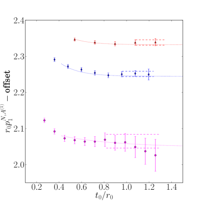
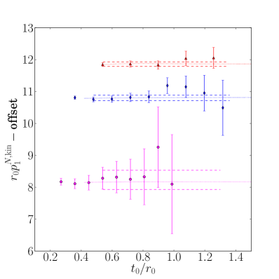
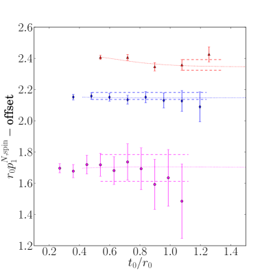
Figure 1: Illustration of some plateaux. Top: $p_{1}^{N,\rm stat}$ (left) and $p_{1}^{N,A^{(1)}}$ (right); bottom $p_{1}^{N,\rm kin}$ (left) and $p_{1}^{N,\rm spin}$ (right). In each plot, the lattice spacing is decreasing from top to bottom. Dotted lines represent the global fit, while dashed lines indicate the chosen plateau. In the plots, $N=5$ and $t-t_{0}=3a$.

3.3 Continuum limit

From the bare matrix elements and the parameters of HQET, determined in [?] with the HYP1 and HYP2 static actions, we form dimensionless quantities

$$\tilde{\Phi}^{\mathrm{stat}}_{n}= \log\left(r_{0}^{3/2}\Phi^{\mathrm{stat}}_{n}\right/\sqrt{2}) =\log Z_{\rm A}^{\mathrm{stat}}+\log(r_{0}^{3/2}p^{\mathrm{stat}}_{n})\;,$$ (3.28)

$$\tilde{\Phi}^{\mathrm{stat},\rm imp}_{n}= \log\left(r_{0}^{3/2}\Phi^{\mathrm{stat},\rm imp}_{n}/\sqrt{2}\right) =\log Z_{\rm A}^{\mathrm{stat},\rm imp}+\log(r_{0}^{3/2}p^{\mathrm{stat}}_{n})$$

$$+c_{\rm A}^{\rm stat}ap_{n}^{A^{(1)}}+b_{\rm A}^{\rm stat}am_{\rm q}\;,$$

$$\tilde{\Phi}^{\rm HQET}_{1}= \log\left(r_{0}^{3/2}\Phi^{\rm HQET}_{1}/\sqrt{2}\right) =\tilde{\Phi}^{\mathrm{stat}}_{1}+b_{\rm A}^{\rm stat}am_{\rm q}+\log Z_{\rm A}^{1/m}$$

$$+\omega_{\rm kin}p_{1}^{\rm kin}+\omega_{\rm spin}p_{1}^{\rm spin}+c_{\rm A}^{(1)}p_{1}^{A^{(1)}}\,,$$

in which the divergences cancel exactly to order ${\rm O}(1/m_{\mathrm{b}})$, and use them to compute $f^{\rm x}_{\rm B_{s}}=\Phi^{\rm x}_{1}/\sqrt{m_{\rm B_{s}}}$.

For a comparison to the static limit and previous work, we also consider

$$\tilde{\Phi}^{\rm RGI}_{1}= \log\left(r_{0}^{3/2}\Phi^{\rm RGI}_{1}/\sqrt{2}\right) =\log Z_{\rm A,RGI}^{\rm stat}+\log(r_{0}^{3/2}p^{\mathrm{stat}}_{1})+c_{\rm A}^{\rm stat}ap_{1}^{{\rm A}^{(1)}}\;,$$ (3.31)

where $Z_{\rm A,RGI}^{\rm stat}$ is the renormalization factor of the Renormalization Group Invariant static-light axial current, as defined in [?]. In contrast to $Z_{\rm A,RGI}^{\rm stat}$, the HQET parameter $Z_{\rm A}^{\rm stat}$ in eq. (3.28) has been determined by a non-perturbative matching at finite mass. The correspondence is

$$Z_{\rm A}^{\rm stat}=Z_{\rm A,RGI}^{\rm stat}\,C_{\rm PS}(M_{\rm b}/\Lambda)\;,$$ (3.32)

in terms of the conversion function $C_{\rm PS}$ introduced in [?] and now known up to three-loops [?,?,?]. For $Z_{\rm A,RGI}^{\rm stat}$ we use the non-perturbative value from [?].

Since both of the static actions used are discretizations of the same continuum theory, we perform a combined continuum limit by fitting a function of the form ($k=1,2$ for HYP1, HYP2 actions)

$$\Psi_{i,k}(a/r_{0})=A_{i}+B_{i,k}\cdot(a/r_{0})^{s_{i}}\,.$$ (3.33)

For $\Psi_{i}\in\{\tilde{\Phi}^{\mathrm{stat},\rm imp}_{1},r_{0}^{3/2}\Phi^{\mathrm{stat},\rm imp}_{1},\tilde{\Phi}^{\rm RGI}_{1},r_{0}^{3/2}\Phi^{\rm RGI}_{1}\}$, we use $s_{i}=2$ because the static axial current has been ${\rm O}(a)$-improved using the coefficients $c_{\rm A}^{\rm stat}$ given in [?] for the actions HYP1 and HYP2. For $\Psi_{i}\in\{\tilde{\Phi}^{\rm HQET}_{1},r_{0}^{3/2}\Phi^{\rm HQET}_{1}\}$, the ${\rm O}(a)$ corrections are suppressed by $1/m_{\mathrm{b}}$, and given the flatness of the observables in $a$, we feel justified in employing $s_{i}=2$ in this case, too.

To estimate the systematic error on $r_{0}^{3/2}\Phi^{\mathrm{stat},\rm imp}_{1}$ incurred from using the one-loop value of $c_{\rm A}^{\rm stat}$, we compute the continuum limit also for $c_{\rm A}^{\rm stat}=0$ using a quadratic extrapolation and compare the result to the continuum limit obtained using the one-loop value. As can be seen from table 3, the influence of $c_{\rm A}^{\rm stat}$ is negligible at this level.

Statistical errors are computed by a jackknife analysis that also includes the correlation among HQET parameters. We find that the results obtained from taking the continuum limit of $\tilde{\Phi}^{\rm x}_{n}$ and using it to compute $\Phi^{\rm x}_{n}$, and from taking the continuum limit of $\Phi^{\rm x}_{n}$ directly agree well within the errors.

		$\beta=6.0219$	$\beta=6.2885$	$\beta=6.4956$	cont. limit
$r_{0}^{3/2}\Phi^{\mathrm{stat}}_{1}$	HYP1	2.30(4)	2.22(4)	2.19(4)	2.14(4)
	HYP2	2.19(3)	2.16(4)	2.15(4)
$r_{0}^{3/2}\Phi^{\mathrm{stat},\rm imp}$	HYP1	2.31(3)	2.22(3)	2.19(4)	2.15(4)
	HYP2	2.23(3)	2.18(3)	2.16(3)
$r_{0}^{3/2}\Phi^{\rm HQET}_{1}$	HYP1	1.96(4)	2.02(4)	1.94(5)	2.02(4)
	HYP2	2.00(3)	2.02(4)	2.04(5)
$r_{0}^{3/2}\Phi^{\rm RGI}_{1}$	HYP1	1.95(3)	1.87(3)	1.85(3)	1.80(3)
($c_{\rm A}^{\rm stat}=0$)	HYP2	1.87(3)	1.83(3)	1.81(3)
$r_{0}^{3/2}\Phi^{\rm RGI}_{1}$	HYP1	1.96(3)	1.88(3)	1.85(3)	1.81(3)
(1-loop $c_{\rm A}^{\rm stat}$)	HYP2	1.90(3)	1.84(3)	1.82(3)

Table 3: The matrix elements in units of the scale $r_{0}$. Shown are the results at each $\beta$ for both static-quark actions, together with their common continuum limit. Note that to compare $\Phi_{1}^{{\rm RGI}}$ with the first three continuum-limit results one has to consider the combination $C_{\rm PS}\times\Phi_{1}^{{\rm RGI}}=2.20(4)$ (1-loop $c_{\rm A}^{\rm stat}$). Here the conversion function $C_{\rm PS}$ [?,?] has been computed with the three-loop anomalous dimension from [?,?].

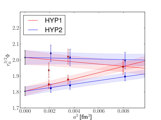
Figure 2: Extrapolation to the continuum limit of $\Phi_{1}^{{\rm RGI}}$ (circles) and $\Phi_{1}^{\rm HQET}$ (diamonds).

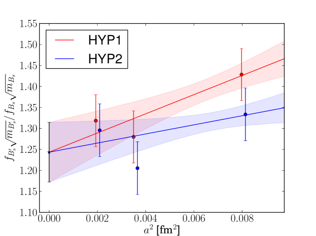
Figure 3: Extrapolation to the continuum limit of $f_{\rm B^{\prime}_{\rm s}}^{\rm stat}\sqrt{m_{\rm B^{\prime}_{\rm s}}}/(f_{\rm B_{\rm s}}^{\rm stat}\sqrt{m_{\rm B_{\rm s}}})$.

In Figures 2 and 3, we show the continuum extrapolations of some relevant quantities. It is easily seen on those plots that the combination of HYP1 and HYP2 results is legitimate because they point to the same continuum limit within the errors.

Numerically we finally get:

$$r_{0}^{3/2}\,f^{\rm stat}_{\rm B_{\rm s}}\sqrt{m_{\rm B_{s}}} = 2.14(4)\,,$$ (3.34)

$$r_{0}^{3/2}\,f^{\rm HQET}_{\rm B_{\rm s}}\sqrt{m_{\rm B_{s}}} = 2.02(5)\,.$$ (3.35)

For $r_{0}=0.5$ fm, our results correspond to $f^{\rm stat}_{\rm B_{\rm s}}=229(3)$ MeV and $f^{\rm HQET}_{\rm B_{\rm s}}=216(5)$ MeV, and for $r_{0}=0.45$ fm to $f^{\rm stat}_{\rm B_{\rm s}}=269(4)$ MeV and $f^{\rm HQET}_{\rm B_{\rm s}}=252(7)$ MeV.

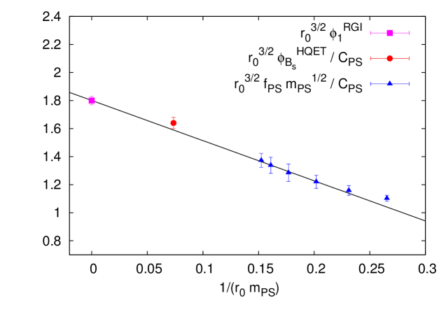
Figure 4: Comparison between our estimation of $\Phi^{\rm HQET}_{\rm B_{s}}=f^{\rm HQET}_{\rm B_{s}}\,\sqrt{m_{\rm B_{s}}}$ and the interpolation at $m_{\rm B_{s}}$ of $f^{\rm stat}_{\rm B_{s}}$ and $f_{\rm D_{s}}$ for a range of $\rm D_{s}$ masses [?]. The notations are explained in the text.

Although our direct computation of $f_{\rm B_{s}}$ in HQET avoids any interpolation (or extrapolation) in the heavy mass, we show in Figure 4 a comparison of our HQET result with an interpolation between previous results for $f_{\rm D_{s}}$ [?] and the static value. As the decay constant itself does not have a well defined infinite mass limit, in the figure we plot the quantity $r_{0}^{3/2}{{f_{\rm PS}\sqrt{m_{\rm PS}}}\over{C_{\rm PS}(M/\Lambda_{\overline{\rm MS}})}}$, by properly rescaling our non-perturbative result for $\Phi_{1}^{\rm HQET}$ (red circle in Figure 4) and the non-perturbative result in [?] for the decay constant around the charm quark mass (blue triangles in Figure 4). The static limit of this quantity is $r_{0}^{3/2}\Phi_{1}^{\rm RGI}$, which we have also non-perturbatively computed here (purple square in Figure 4). As explained above we rely on perturbation theory only for the evaluation of the conversion function $C_{\rm PS}(M/\Lambda_{\overline{\rm MS}})$ relating the RGI matrix elements in static HQET with their counterpart in QCD defined at a given heavy quark mass [?,?]. Thus, dividing by $C_{\rm PS}(M_{\rm b}/\Lambda_{\overline{\rm MS}})$ compensates for the well-known logarithmic scaling of the decay constant with the heavy-quark mass [?,?]. One can see that our result is falling rather well on the straight line expected from heavy quark scaling, indicating that the neglected ${\rm O}(1/m_{\mathrm{b}}^{n})|_{n\geq 2}$ corrections are small. We note, however, that this comparison and conclusion rely on the perturbative evaluation of $C_{\rm PS}$, and that the associated $\alpha_{\mathrm{s}}(m)^{3}$ errors are very difficult to estimate.

Our use of the GEVP method also allows us to extract some information on the matrix element for $n=2$, i.e. of the first excited state of the $\rm B_{s}$ system, for which we obtain

$${f^{\rm stat}_{\rm B^{\prime}_{\rm s}}\sqrt{m_{\rm B^{\prime}_{s}}}\over f^{\rm stat}_{\rm B_{\rm s}}\sqrt{m_{\rm B_{s}}}}=1.24(7)$$ (3.36)

from the ratio ${{p^{\rm stat}_{2}(1+c_{\rm A}^{\rm stat}p_{2}^{\rm A^{(1)}})}\over{p^{\rm stat}_{1}(1+c_{\rm A}^{\rm stat}p_{1}^{\rm A^{(1)}})}}$ quadratically extrapolated to the continuum limit. The unimproved version of this quantity (i.e. $p^{\rm stat}_{2}/p^{\rm stat}_{1}$), quadratically extrapolated to the continuum, gives the same result of 1.24(7). We have obtained the same qualitative result as [?] concerning this ratio: it is noticeably larger than 1, in good qualitative agreement with predictions from quark models that become Lorentz covariant in the heavy quark limit [?] and relativistic quasi-potential quark models [?,?], while other models predict a value less than 1 for this quantity [?].

4 Conclusion

In this paper we have reported on the computation of the $\rm B_{\rm s}$ meson decay constant by using lattice simulations in quenched HQET. Including $1/m_{\mathrm{b}}$ corrections introduces power divergences $\sim 1/(am_{{\rm b}})$ which have to be subtracted non-perturbatively. These non-perturbative subtractions have here been carried out successfully for the first time in lattice gauge theory computations. The necessary couplings of the effective theory had been determined non-perturbatively by matching it to QCD [?].

Our strategy had already been developed earlier [?] but its implementation revealed relatively large statistical errors in the matrix elements of the $1/m_{\mathrm{b}}$ operators (not due to the computation of the non-perturbative parameters of the theory). This shortcoming has now been cured by exploiting (i) a method based on solving a GEVP to reduce the systematic errors on bare matrix elements coming from the contribution of excited states to correlation functions and (ii) all-to-all propagators to improve the statistical precision. For example, at the finest lattice resolution considered, we have obtained a result for the bare static decay constant (HYP2 action), which is three times more precise than the result in [?] at $\beta=6.45$ where ten times more configurations were analyzed in the Schrödinger Functional setup.

We used three lattice spacings to extrapolate to the continuum limit. With $r_{0}=0.5$ fm we have obtained $f^{\rm stat,N_{\rm f}=0}_{\rm B_{\rm s}}=229(3)$ MeV and $f^{\rm HQET,N_{\rm f}=0}_{\rm B_{\rm s}}=216(5)$ MeV. Thus the relative $1/m_{\mathrm{b}}$ corrections are small as expected from simple estimates such as $400\,{\rm MeV}/m_{{\rm b}}$ and we have found evidence that ${\rm O}(1/m_{\mathrm{b}}^{2})$ corrections are very small. In addition, we have shown that the GEVP method is useful for studying phenomenologically interesting quantities involving radial excitations of mesonic states, such as the ratio $f_{\rm B^{\prime}_{\rm s}}/f_{\rm B_{\rm s}}$. In this respect we confirm a recent lattice calculation [?] finding that $f_{\rm B^{\prime}_{\rm s}}/f_{\rm B_{\rm s}}>1$ at least in the static approximation.

We intend to apply the approach described in this paper to the computation of $f_{\rm B_{\rm s}}$ and $f_{\rm B}$ on dynamical $N_{\rm f}=2$ configurations in the near future. Note that the problem posed for charm physics on the lattice by the rapid slowing-down of the topological modes of the gauge fields with decreasing lattice spacing [?,?,?] is less relevant in this case, since in HQET we can afford to work with coarser lattices.

Acknowledgements. We thank NIC for allocating computer time on the APE computers and the computer farm at DESY, Zeuthen, and the staff of the computer center at Zeuthen for their support. This work is supported by the Deutsche Forschungsgemeinschaft in the SFB/TR 09, and by the European community through EU Contract No. MRTN-CT-2006-035482, “FLAVIAnet”. N.G. acknowledges financial support from the MICINN grant FPA2006-05807, the Comunidad Autónoma de Madrid programme HEPHACOS P-ESP-00346, and participates in the Consolider-Ingenio 2010 CPAN (CSD2007-00042). T.M. thanks the A. von Humboldt Foundation for support.

References

- [1] M. Antonelli et al., Flavor Physics in the Quark Sector, 0907.5386.
- [2] M. Misiak and J. Urban, QCD corrections to FCNC decays mediated by Z-penguins and W-boxes, Phys. Lett. B451 (1999) 161–169, [hep-ph/9901278].
- [3] G. Buchalla and A. J. Buras, The rare decays , and : An update, Nucl. Phys. B548 (1999) 309–327, [hep-ph/9901288].
- [4] A. J. Buras, Relations between and in models with minimal flavor violation, Phys. Lett. B566 (2003) 115–119, [hep-ph/0303060].
- [5] D0 Collaboration, V. M. Abazov et al., Search for the rare decay , Phys. Lett. B693 (2010) 539–544, [1006.3469].
- [6] K. S. Babu and C. F. Kolda, Higgs mediated in minimal supersymmetry, Phys. Rev. Lett. 84 (2000) 228–231, [hep-ph/9909476].
- [7] LHCb Collaboration, P. Perret et al., Prospects for New Physics in CP Violation and Rare Decays at LHCb, 0901.2856.
- [8] M. Della Morte, Standard Model parameters and heavy quarks on the lattice, PoS LAT2007 (2007) 008, [0711.3160].
- [9] E. Gamiz, Heavy flavour phenomenology from lattice QCD, PoS LATTICE2008 (2008) 014, [0811.4146].
- [10] E. Eichten and B. R. Hill, An Effective Field Theory for the Calculation of Matrix Elements Involving Heavy Quarks, Phys. Lett. B234 (1990) 511.
- [11] E. Eichten and B. R. Hill, Static effective field theory: 1/m corrections, Phys. Lett. B243 (1990) 427–431.
- [12] ALPHA Collaboration, B. Blossier, M. Della Morte, N. Garron, and R. Sommer, HQET at order : I. Non-perturbative parameters in the quenched approximation, JHEP 06 (2010) 002, [1001.4783].
- [13] ALPHA Collaboration, B. Blossier, M. Della Morte, N. Garron, and R. Sommer, Heavy-light decay constant at the 1/m order of HQET, PoS LAT2007 (2007) 245, [0710.1553].
- [14] ALPHA Collaboration, B. Blossier, M. Della Morte, G. von Hippel, T. Mendes, and R. Sommer, On the generalized eigenvalue method for energies and matrix elements in lattice field theory, JHEP 04 (2009) 094, [0902.1265].
- [15] ALPHA Collaboration, M. Kurth and R. Sommer, Renormalization and O()-improvement of the static axial current, Nucl. Phys. B597 (2001) 488–518, [hep-lat/0007002].
- [16] C. Michael and I. Teasdale, Extracting glueball masses from lattice qcd, Nucl. Phys. B215 (1983) 433–446.
- [17] M. Lüscher and U. Wolff, How to calculate the elastic scattering matrix in two-dimensional quantum field theories by numerical simulation, Nucl. Phys. B339 (1990) 222–252.
- [18] ALPHA Collaboration, A. Grimbach, D. Guazzini, F. Knechtli, and F. Palombi, O(a) improvement of the HYP static axial and vector currents at one-loop order of perturbation theory, JHEP 03 (2008) 039, [0802.0862].
- [19] A. Hasenfratz and F. Knechtli, Flavor symmetry and the static potential with hypercubic blocking, Phys. Rev. D64 (2001) 034504, [hep-lat/0103029].
- [20] A. Hasenfratz, R. Hoffmann, and F. Knechtli, The static potential with hypercubic blocking, Nucl. Phys. Proc. Suppl. 106 (2002) 418–420, [hep-lat/0110168].
- [21] ALPHA Collaboration, M. Della Morte, A. Shindler, and R. Sommer, On lattice actions for static quarks, JHEP 08 (2005) 051, [hep-lat/0506008].
- [22] B. Sheikholeslami and R. Wohlert, Improved continuum limit lattice action for QCD with Wilson fermions, Nucl. Phys. B259 (1985) 572.
- [23] M. Lüscher, S. Sint, R. Sommer, P. Weisz, and U. Wolff, Non-perturbative O(a) improvement of lattice QCD, Nucl. Phys. B491 (1997) 323–343, [hep-lat/9609035].
- [24] TrinLat Collaboration, J. Foley et al., Practical all-to-all propagators for lattice QCD, Comput. Phys. Commun. 172 (2005) 145–162, [hep-lat/0505023].
- [25] ALPHA Collaboration, B. Blossier et al., HQET at order : II. Spectroscopy in the quenched approximation, JHEP 05 (2010) 074, [1004.2661].
- [26] ALPHA Collaboration, M. Guagnelli, R. Sommer, and H. Wittig, Precision computation of a low-energy reference scale in quenched lattice QCD, Nucl. Phys. B535 (1998) 389–402, [hep-lat/9806005].
- [27] ALPHA Collaboration, J. Garden, J. Heitger, R. Sommer, and H. Wittig, Precision computation of the strange quark’s mass in quenched QCD, Nucl. Phys. B571 (2000) 237–256, [hep-lat/9906013].
- [28] S. Güsken et al., Nonsinglet Axial Vector Couplings of the Baryon Octet in Lattice QCD, Phys. Lett. B227 (1989) 266.
- [29] APE Collaboration, M. Albanese et al., Glueball masses and string tension in lattice QCD, Phys. Lett. 192B (1987) 163.
- [30] S. Basak et al., Combining Quark and Link Smearing to Improve Extended Baryon Operators, PoS LAT2005 (2006) 076, [hep-lat/0509179].
- [31] ALPHA Collaboration, J. Heitger, M. Kurth, and R. Sommer, Non-perturbative renormalization of the static axial current in quenched QCD, Nucl. Phys. B669 (2003) 173–206, [hep-lat/0302019].
- [32] ALPHA Collaboration, J. Heitger, A. Jüttner, R. Sommer, and J. Wennekers, Non-perturbative tests of heavy quark effective theory, JHEP 11 (2004) 048, [hep-ph/0407227].
- [33] K. G. Chetyrkin and A. G. Grozin, Three-loop anomalous dimension of the heavy-light quark current in HQET, Nucl. Phys. B666 (2003) 289–302, [hep-ph/0303113].
- [34] S. Bekavac et al., Matching QCD and HQET heavy-light currents at three loops, Nucl. Phys. B833 (2010) 46–63, [0911.3356].
- [35] M. Della Morte et al., Heavy-strange meson decay constants in the continuum limit of quenched QCD, JHEP 02 (2008) 078, [0710.2201].
- [36] M. A. Shifman and M. B. Voloshin, On Annihilation of Mesons Built from Heavy and Light Quark and Oscillations, Sov. J. Nucl. Phys. 45 (1987) 292.
- [37] H. D. Politzer and M. B. Wise, Leading Logarithms of Heavy Quark Masses in Processes with Light and Heavy Quarks, Phys. Lett. B206 (1988) 681.
- [38] T. Burch, C. Hagen, C. B. Lang, M. Limmer, and A. Schäfer, Excitations of single-beauty hadrons, Phys. Rev. D79 (2009) 014504, [0809.1103].
- [39] V. Morénas, A. Le Yaouanc, L. Oliver, O. Pène, and J. C. Raynal, Decay constants in the heavy quark limit in models à la Bakamjian and Thomas, Phys. Rev. D58 (1998) 114019, [hep-ph/9710298].
- [40] D. Ebert, V. O. Galkin, and R. N. Faustov, Mass spectrum of orbitally and radially excited heavy- light mesons in the relativistic quark model, Phys. Rev. D57 (1998) 5663–5669, [hep-ph/9712318].
- [41] D. Ebert, R. N. Faustov, and V. O. Galkin, Decay constants of heavy-light mesons in the relativistic quark model, Mod. Phys. Lett. A17 (2002) 803–808, [hep-ph/0204167].
- [42] A. M. Badalian, B. L. G. Bakker, and Y. A. Simonov, Decay constants of the heavy-light mesons from the field correlator method, Phys. Rev. D75 (2007) 116001, [hep-ph/0702157].
- [43] L. Del Debbio, H. Panagopoulos, and E. Vicari, theta dependence of SU() gauge theories, JHEP 0208 (2002) 044, [hep-th/0204125].
- [44] L. Del Debbio, G. M. Manca, and E. Vicari, Critical slowing down of topological modes, Phys. Lett. B594 (2004) 315–323, [hep-lat/0403001].
- [45] S. Schaefer, R. Sommer, and F. Virotta, Investigating the critical slowing down of QCD simulations, 0910.1465.