The Abelian Manna model on two fractal lattices

Abstract

We analyze the avalanche size distribution of the Abelian Manna model on two different fractal lattices with the same dimension $d_{g}=\ln 3/\ln 2$, with the aim to probe for scaling behavior and to study the systematic dependence of the critical exponents on the dimension and structure of the lattices. We show that the scaling law $D(2-\tau)=d_{w}$ generalizes the corresponding scaling law on regular lattices, in particular hypercubes, where $d_{w}=2$. Furthermore, we observe that the lattice dimension $d_{g}$, the fractal dimension of the random walk on the lattice $d_{w}$, and the critical exponent $D$, form a plane in $3D$ parameter space, i.e. they obey the linear relationship $D=0.632(3)d_{g}+0.98(1)d_{w}-0.49(3)$.

Although extensive research has been performed on self-organized criticality Bak et al. (1987) for models on hypercubic lattices, far less work has been done on fractal lattices Kutnjak-Urbance et al. (1996); Lee et al. (2009). It remains somewhat unclear what to conclude from the latter studies. Fractal lattices are important for the understanding of critical phenomena for a number of reasons. Firstly, results for critical exponents in lattices with non-integer dimensions might provide a means to determine the terms of their $\epsilon=4-d$ expansion. Secondly, fractal lattices are particularly suitable for a real space renormalization group procedures, in particular that by Migdal and Kadanoff Migdal (1976); Kadanoff (1976); Carmona et al. (1998). Thirdly, scaling relations that are derived in a straightforward fashion on hypercubic lattices can be put to test in a more general setting. In this Brief Report, we address the first and the third aspect, by examining both numerically and analytically the scaling behaviour of the Abelian version of the Manna model (Manna, 1991; Dhar, 1999, 2006) on two different fractal lattices.

The fractal lattices used in this study are generated from the arc-fractal system Huynh and Chew (2010). The lattice sites are the invariant set of points of the arc-fractal. We consider nearest neighbor interactions among sites. Here, the nearest neighbors of a given site are all sites which have the (same) shortest Euclidean distance to it. Our fractal lattices have no natural boundary; instead, they have only two end points at which two copies can join to form a bigger lattice. The dimension of the lattices is the same as the arc-fractal that generates them.

In this study, we shall consider two fractal lattices: the Sierpinski arrowhead and the crab (see Fig. 1). The former is named “Sierpinski arrowhead” because it is the same as the well-known Sierpinski arrowhead Mandelbrot (1982), whereas the latter is termed “crab” because the overall shape of the generated lattice looks like a crab. These fractal lattices are generated through the arc-fractal system with number of segments $n=3$ and opening angle of the arc $\alpha=\pi$. For the Sierpinski arrowhead, the rule for orientating the arc at each iteration is “in-out-in”, while the rule is “out-in-out” for the crab. Both lattices have the same dimension $d_{g}=\ln 3/\ln 2\approx 1.58$. The total number of sites on the lattice at the $i$-th iteration is $N_{i}=3^{i}+1$. The coordination number of sites on these lattices varies between two and three. Asymptotically, one-third of the sites have three nearest neighbors (called extended sites), while the remaining two thirds have two nearest neighbors (called normal sites). Since the lattice sites are being stringed up by arcs (see Fig. 1), they can be labeled as sites on a $1D$ linear chain. In order to determine the linear size (to be used in finite size scaling) of the lattice, reference sites (hollow circles, which are not part of the lattice) have been added between the real sites (solid circles). This is possible because of the uniform spacing between sites. The linear size is then equal to the total number of hollow and solid circles along $L$ (see Fig. 1). At the $i$-th iteration, the linear size is given by $L_{i}=2^{i}+1$ for the arrowhead lattice and $L_{i}=3\times 2^{i-1}$ for the crab lattice. Indeed, one observes that the dimension of the lattice obeys the following relation with the total number of sites and linear size of the lattice: $d_{g}=\lim_{i\rightarrow\infty}\ln{N_{i}}/\ln{L_{i}}$.

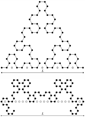
Figure 1: Sierpinski arrowhead (top) and crab (bottom) lattice at $4^{th}$ iteration with definition of linear size. In the figure, $L=17$ for arrowhead and $L=24$ for crab lattice.

We implement the Abelian Manna model on these two fractal lattices that have the same dimension but possess different microscopic structures. Let us denote the variable $z_{j}$, which is a non-negative integer, to be the “height” or the number of particles at lattice site $j$. The lattice is first initialized with $z_{j}=0$ for all sites. The value of $z_{j}$ is then evolved according to the following algorithm. When the system is in a stable configuration, i.e. $z_{j}\leq 1$ for all sites, the external drive is implemented by picking a site $j$ at random and increasing its $z_{j}$ by one unit. At this juncture, an avalanche might occur in the following manner: as long as there exist any $j$ with $z_{j}$ exceeding the threshold $z_{c}=1$ (an “active” site), pick one of them at random, say $k$, and reduce $z_{k}$ by two. At the same time, pick two of its nearest neighbours, say $k^{\prime}$, randomly and independently, and increment $z_{k^{\prime}}$ by one unit. This procedure constitutes a toppling, which in the bulk is conservative, i.e. the total $\sum_{j}z_{j}$ remains unchanged by the bulk topplings. In one dimension, every bulk site has two neighbours. On the fractal lattices described above, a bulk site can have either two or three nearest neighbours. Note that particles can leave the system at the two end sites (labeled as $1$ and $3^{i}+1$ respectively). Owing to the Abelianess of the model, the statistics of the avalanche sizes is independent from the order of updates. This is different for time-dependent observables such as the avalanche duration, which is not studied in the following.

An avalanche ceases as soon as $z_{j}\leq 1$ for all $j$ (quiescence). The size $s$ of the avalanche is measured as the number of topplings performed between two quiescent configurations. The probability density $\mathcal{P}\left(s\right)$ for an avalanche of size $s$ to occur is expected to follow simple (finite size) scaling

$$\mathcal{P}\left(s\right)=as^{-\tau}\mathcal{G}\left(\frac{s}{bL^{D}}\right)$$ (1)

asymptotically in large $s\gg s_{0}$ with lower cutoff $s_{0}$, linear system size $L$, non-universal metric factors $a$ and $b$ and universal exponents $\tau$ and $D$. The universal scaling function $\mathcal{G}$ decays, for large arguments, faster than any power law, so that all moments

$$\left\langle s^{q}\right\rangle=\int\mathchoice{\!\mathrm{d}s\,}{\!\mathrm{d}s\,}{\!\mathrm{d}s\,}{\!\mathrm{d}s\,}\mathcal{P}\left(s\right)s^{q}$$ (2)

exist for any finite system. Provided that $q+1-\tau>0$ one can easily show that

$$\left\langle s^{q}\right\rangle\propto L^{D(q+1-\tau)}\ .$$ (3)

The results presented in the following are based on Monte Carlo simulations for four different system sizes, corresponding to four different levels of iteration $i=3,4,5,6$, containing $N=28,82,244,730$ sites and with linear size $L=9,17,33,65$ for the Sierpinski arrowhead lattice and $L=12,24,48,96$ for the crab lattice. In all four cases, $10^{8}$ avalanches were triggered and the data recorded in regular intervals of $10^{6}$ avalanches. Stationarity was verified by inspecting avalanche size moments and the transient was determined to be shorter than $5\cdot 10^{4}$ avalanches. Errors for the moments are derived from a Jackknife estimator Efron (1982); Berg (1992) of the variance based on the moments taken in each set of $10^{6}$ measurements. The scaling exponents were determined by a nonlinear least square fitting Press et al. (2007) of the avalanche size moments against the linear size of the lattice:

$$\left\langle s^{q}\right\rangle=\left(a_{q}+\frac{b_{q}}{L}+\frac{c_{q}}{L^{2}}\right)L^{D(q+1-\tau)}\ .$$ (4)

The exponents derived in this procedure were $\tau=1.170(5)$ and $D=2.792(2)$ for the arrowhead lattice; and $\tau=1.153(4)$ and $D=3.026(2)$ for the crab lattice.

In addition, the scaling behaviour can be probed in a data collapse, as illustrated in Fig. 2.

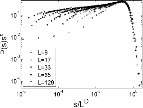
Figure 2: Data collapse of binned data for Sierpinski arrowhead lattice. Preliminary statistics of large system size ($7^{th}$ iteration, $L=129$) are also included to test the consistency of the data. The plots confirm the estimated values of the critical exponents.

With the critical exponents determined, one can immediately verify the scaling law of avalanche size distribution. From hypercubic lattices it is well known Nakanishi and Sneppen (1997) that the first moment of the avalanche size is given by the expected number of moves that a random walker performs on the given lattice before it reaches the boundary and leaves, i.e. by its residence time. This is essentially because of bulk conservation: In the stationary state one particle leaves the system for every particle added (avalanche attempt) and the average number of moves it performs during its residency is exactly twice the average number of topplings occuring in the system per particle added, which is the avalanche size. Regardless of the specifics of the boundary, i.e. regardless of whether only two sites are dissipative or all sites along the perimeter, the first moment normally scales with the linear size of the lattices squared, $D(2-\tau)=2$, independent from the dimension of the hypercubic lattice. This is easily understood, as the time and thus the total number of moves performed by a random walker scales quadratically in the linear distance traversed.

For the fractal lattices, it is obvious that $D(2-\tau)$ is not equal to 2 since it is $2.317(8)$ for the arrowhead lattice and $2.564(6)$ for the crab lattice. We will now show that the scaling law has in fact changed to $D(2-\tau)=d_{w}$, where $d_{w}$ is the fractal dimension of random walk on the lattice. The scale law $D(2-\tau)=d_{w}$ remains true for any lattice regardless of dimension and microscopic details.

We will now calculate $d_{w}$ for the Sierpinski arrowhead lattice and the crab lattice by using the first-passage time method Avraham and Havlin (2000). Due to the nearest neighbor structure of the fractal lattices, the calculation is not coarse-grained renormalization-like, but rather, it is carried out by considering every single edge that connects between the two end sites on the lattice.

We label the sites of the lattice sequentially with $j=1,2,\cdots,3^{i}+1$ and denote by $T_{j}^{(i)}$ the average time for the random walker to exit through the end sites from site $j$ ($i$ is the number of iterations of the lattice). Also, we denote by $t$ the traverse time from one site to its nearest neighbor.

Let us define $E^{(i)}$ to be the set of extended sites at the $i$-th iteration. On the lattice, each normal site $j$ has two nearest neighbors $j-1$ and $j+1$. If $j$ is an extended site, it has in addition a third nearest neighbor $j^{*}$. If the walker is at site $j$, we have 2 situations:

If $j\not\in E^{(i)}$, the walker has only 2 options to choose from: go to $j-1$ or go to $j+1$. The probability for each choice is $1/2$. We have

$$T_{j}^{(i)} = \frac{1}{2}\left(t+T_{j-1}^{(i)}\right)+\frac{1}{2}\left(t+T_{j+1}^{(i)}\right)$$ (5)

$$= t+\frac{1}{2}T_{j-1}^{(i)}+\frac{1}{2}T_{j+1}^{(i)}\ .$$

If $j\in E^{(i)}$, the walker has up to 3 options to choose from: go to $j-1$, go to $j+1$ or go to $j^{*}$. The probability for each choice is $1/3$. Thus we have

$$T_{j}^{(i)} = \frac{1}{3}\left(t+T_{j-1}^{(i)}\right)+\frac{1}{3}\left(t+T_{j+1}^{(i)}\right)+\frac{1}{3}\left(t+T_{j^{*}}^{(i)}\right)$$ (6)

$$= t+\frac{1}{3}T_{j-1}^{(i)}+\frac{1}{3}T_{j+1}^{(i)}+\frac{1}{3}T_{j^{*}}^{(i)}\ .$$

Since this gives a system of linear equations, we can write them in the form of a matrix equation: $A^{(i)}T^{(i)}=B^{(i)}$, where $T^{(i)}$ is the column vector of $T_{j}^{(i)}$, $A^{(i)}$ is the degree-normalised adjacency matrix, while $B^{(i)}$ is a column vector contains $t$ in every entry. As $A^{(i)}$ is invertible, we can solve for $T^{(i)}=\left(A^{(i)}\right)^{-1}B^{(i)}$. By defining the new variable: $S_{j}^{(i)}=T_{j}^{(i+1)}/T_{j}^{(i)}$, we obtain the results as shown in Table 1 for the arrowhead lattice and the crab lattice.

Table 1: Convergence of $S_{1}^{(i)}$ as the number of iterations $i$ increases. After $i=7$, we have $S_{1}^{(i)}\approx 5$ for the Sierpinski arrowhead lattice and $S_{1}^{(i)}\approx 6$ for the crab lattice. Other $S_{j}^{(i)}$’s are found to converge to the same limits.

$i$	1	2	3	4	5	6	7
Arrowhead	11	5.5076	4.7553	4.8806	4.9610	4.9893	4.9974
Crab	10	7.1417	6.9528	6.3729	6.1014	6.0303	5.9727

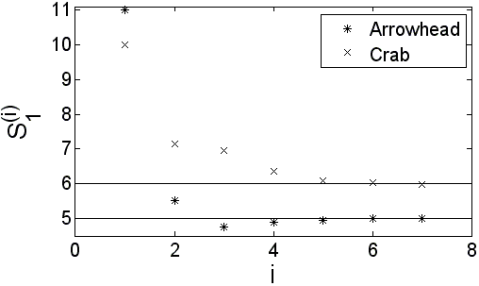
Figure 3: Convergence of $S_{1}^{(i)}$ as number of iterations $i$ increases. After $i=7$ we have $S_{1}^{(i)}=5$ for arrowhead lattice and $S_{1}^{(i)}\approx 6$ for crab lattice. Other $S_{j}^{(i)}$’s converge to the same limits.

We observe that for both lattices $S_{j}^{(i)}$ converges to some value $S_{j}^{*}$ as $i$ increases. For the arrowhead lattice, $S_{j}^{*}=5$, while for the crab lattice, $S_{j}^{*}\approx 6$. On going from the $i$-th to $(i+1)$-th iteration, the lattice size increases by a factor $L_{i+1}/L_{i}=2$, while the escape time increases by a factor $T^{(i+1)}/T^{(i)}=S_{j}^{*}$ for large $i$, so that $d_{w}=\ln{S_{j}^{*}}/\ln 2$. By comparing the calculated $d_{w}$ to the estimated value of $D(2-\tau)$ from simulation, we can see that they are in good agreement (see Table 2).

Table 2: The calculated $d_{w}$ and the estimated $D(2-\tau)$ for the Sierpinski arrowhead lattice and the crab lattice.

Lattice	Arrowhead	Crab
$d_{w}$	$2.322$	$2.578$
$D(2-\tau)$	$2.317\pm 0.008$	$2.564\pm 0.006$

One surprising conclusion from the above results is that for two lattices with the same dimension but different microscopic structure, the critical exponents $D$ and $\tau$ can both be different, which suggests that on fractal lattices, the critical exponents depend not only on the dimension but also on the microscopic details of the lattice. In addition, our results have validated the scaling relation $D(2-\tau)=d_{w}$ for two fractal lattices with different $d_{w}$. Since on lattices with integer dimensions $d_{w}=2$ regardless of the lattice’s structure, this scaling relation generalizes the standard version $D(2-\tau)=2$ known for the hypercubic lattices. The last unexpected conclusion pertains to the relation between the dimensions $d_{g}$ and $d_{w}$, and the critical exponent $D$. We found that they obey the general linear relationship: $D=\alpha d_{g}+\beta d_{w}+\gamma$. This was uncovered by plotting the following six points in $3D$ parameter space: $(d_{g},d_{w},D)=(1,2,2.1),(2,2,2.73),(3,2,3.36),(4,2,4)$, $(1.58,2.32,2.79),(1.58,2.58,3.03)$, which correspond to the linear chain Nakanishi and Sneppen (1997), the square Chessa et al. (1999a); Manna (1991), the cube Pastor-Satorras and Vespignani (2001); Ben-Hur and Biham (1996), the hypercube Lübeck (2004), the arrowhead and the crab lattices respectively. It is interesting that while the first four points due to the hypercubic lattices are found to lie on a straight line, all six points together make up a plane instead of a tetrahedron. We have determined the coefficients $\alpha=0.632\pm 0.003$, $\beta=0.980\pm 0.014$ and $\gamma=-0.492\pm 0.034$ from the six points, which leads to the following relationship:

$$D\approx D_{trial}(d_{g},d_{w})=0.632d_{g}+0.980d_{w}-0.492\ .$$ (7)

Table 3: Data for $(d_{g},d_{w},D)$ from 6 different lattices and the calculated $D_{trial}$ from Eq. (7).

Lattices	$1D$	$2D$	$3D$	$4D$	Arrowhead	Crab
$d_{g}$	1	2	3	4	1.58	1.58
$d_{w}$	2	2	2	2	2.32	2.58
$D$	2.2(1)	2.73(2)	3.36(1)	4	2.792(2)	3.026(2)
$D_{trial}$	2.10(7)	2.73(7)	3.36(7)	4.00(7)	2.78(7)	3.03(7)

A comparison of the value of $D$ determined by Eq. (7) and that from the simulation is shown in Table 3.

Finally, we comment on the slight mismatches between the calculated $d_{w}$ and the estimated $D(2-\tau)$ in Table 2. They seem to be caused by finite size corrections, which are further suppressed at $7$ iterations and above, as observed in preliminary data not included in the main analysis above. In the presence of strong finite size corrections and high accuracy measurements of the moments, the estimates for $D$ and $\tau$ are sensitive to the choice of the fitting function, which is constrained by the number of data points (i.e. system sizes) available, but needs to contain as many correction terms as possible to account for the accurate data. Our choice Eq. (4) reflects the desire to reduce the sensitivity of the estimate on the initial values.

It is important to note that there is a level of ambiguity in the finite size scaling in fractal lattices, because due to its highly irregular nature, there is, a priori, no unique way of increasing the lattice size of a fractal Pruessner et al. (2001). At a given level of iterations in order to increase the lattice size further, one might either proceed by iterating the fractal, or use the given fractal to tessellate the hypercubic lattice of appropriate (embedding) dimension. One might argue that finite size scaling is of course sensitive to that choice and as a result, generates asymptotically either the exponents of the fractal lattice or of the embedding space. However, in ordinary critical phenomena, there are cases Pruessner et al. (2001) where the (effective) critical point and even the scaling functions change with the level of iteration $i$. In the current context that translates to, for example, the amplitude $A_{q}=a_{q}+b_{q}/L+c_{q}/L^{2}$ in Eq. (4) to acquire a dependence on $i$, which might distort the resulting estimates. The exponents derived above can thus be seen only as effective exponents of a fractal lattice.

References

- Bak et al. (1987) P. Bak, C. Tang, and K. Wiesenfeld, Phys. Rev. Lett. 59, 381 (1987).
- Kutnjak-Urbance et al. (1996) B. Kutnjak-Urbanc, S. Zapperi, S. Milosevic, and H. E. Stanley, Phys. Rev. E 54, 272 (1996).
- Lee et al. (2009) K. E. Lee, J. Y. Sung, M. Y. Cha, S. E. Maeng, Y. S. Bang, and J. W. Lee, Phys. Lett. A 373, 4260 (2009).
- Migdal (1976) A. A. Migdal, Sov. Phys.-JETP 42, 413 (1976).
- Kadanoff (1976) L. P. Kadanoff, Ann. Phys. 100, 359 (1976).
- Carmona et al. (1998) J. M. Carmona, U. M. B. Marconi, J. J. Ruiz-Lorenzo, and A. Tarancón, Phys. Rev. B 58, 14387 (1998), eprint arXiv:cond-mat/9802018v2.
- Manna (1991) S. S. Manna, J. Phys. A: Math. Gen. 24, L363 (1991).
- Dhar (1999) D. Dhar, Physica A 263, 4 (1999a), proceedings of the 20th IUPAP International Conference on Statistical Physics, Paris, France, Jul 20–24, 1998, eprint arXiv:cond-mat/9808047.
- Dhar (2006) D. Dhar, Physica A 369, 29 (2006), proceedings of the 11th International Summerschool on ’Fundamental Problems in Statistical Physics’, Leuven, Belgium, Sep 4 – 17, 2005.
- Huynh and Chew (2010) H. N. Huynh and L. Y. Chew, submitted to Fractals, unpublished, eprint available on the journal’s world wide web: http://www.worldscinet.com/fractals/editorial/paper/910421.pdf.
- Mandelbrot (1982) B. B. Mandelbrot, The Fractal Geometry of Nature (W. H. Freeman, New York, USA, 1982), pp141-142
- Efron (1982) B. Efron, The Jackknife, the Bootstrap and Other Resampling Plans (SIAM, Philadelphia, PA, USA, 1982).
- Berg (1992) B. A. Berg, Comp. Phys. Comm. 69, 7 (1992).
- Press et al. (2007) W. H. Press, S. A. Teukolsky, W. T. Vetterling, and B. P. Flannery, Numerical Recipes (Cambridge University Press, Cambridge, UK, 2007), 3rd ed.
- Nakanishi and Sneppen (1997) H. Nakanishi and K. Sneppen, Phys. Rev. E 55, 4012 (1997).
- Avraham and Havlin (2000) D. ben-Avraham and S. Havlin, Diffusion and Reactions in Fractals and Disordered Systems (Cambridge University Press, Cambridge, UK, 2000).
- Chessa et al. (1999a) A. Chessa, H. E. Stanley, A. Vespignani, and S. Zapperi, Phys. Rev. E 59, R12 (1999a).
- Pastor-Satorras and Vespignani (2001) R. Pastor-Satorras and A. Vespignani, Eur. Phys. J. B 19, 583 (2001), eprint arXiv:cond-mat/0101358.
- Ben-Hur and Biham (1996) A. Ben-Hur and O. Biham, Phys. Rev. E 53, R1317 (1996).
- Lübeck (2004) S. Lübeck, Int. J. Mod. Phys. B 18, 3977 (2004).
- Pruessner et al. (2001) G. Pruessner, D. Loison, and K.-D. Schotte, Phys. Rev. B 64, 134414 (pages 10) (2001).