Effective Hamiltonian study of excitations in a boson- fermion mixture with attraction between components

Abstract

An effective Hamiltonian for the Bose subsystem in the mixture of ultracold atomic clouds of bosons and fermions with mutual attractive interaction is used for investigating collective excitation spectrum. The ground state and mode frequencies of the ⁸⁷Rb and ⁴⁰K mixture are analyzed quantitatively at zero temperature. We find analytically solutions of the hydrodynamics equations in the Thomas- Fermi approximation. We discuss the relation between the onset of collapse and collective modes softening and the dependence of collective oscillations on scattering length and number of boson atoms.

I Introduction

Bose-Einstein condensation (BEC) in ultracold trapped atomic gases [1] ; [2] ; [3] has been the subject of intense theoretical and experimental interest Bloch08 ; Giorgini08 . Experimental studies of the BEC properties in confined vapours of alkali atoms have been extended to double Bose condensates cr1 ; cr2 ; cr3 ; cr4 , to the achievement of quantal degeneracy in gases of fermionic atoms sci99 , and to dilute mixtures of Bose and Fermi particles sci01 ; prl1 ; NaLi ; Modugno02 ; KRb .

Collisional interaction between bosons and fermions greatly affects the properties and leads to a rich phase diagram of the degenerate mixtures. Theoretical considerations predict the phenomenon of component separation for systems with a positive coupling constant Nygaard99 ; Yi01 ; Minguzzi2000 ; Akdeniz02 ; Capuzzi02 , instabilities and significant modification of the properties of individual component in a case of boson-fermion attraction Roth02 ; Molmer98 ; jezek , the formation of a superfluid state due to boson-induced fermion-fermion attraction Stoof2000 . The simultaneous collapse of the two species has been observed experimentally in the ⁴⁰K - ⁸⁷Rb mixture by Modugno and co-workers Modugno02 as a sudden disappearance of fermion cloud when the number of bosons is increased over an instability value $N_{Bc}\approx 10^{5}$, the critical number of fermions being $N_{K}\approx 2\times 10^{4}$. The stability diagram for the ⁴⁰K - ⁸⁷Rb mixture and the critical particle number for the onset of the collapse has been considered in Ospelkaus06 .

The dynamical properties have been investigated for various boson-fermion mixtures, i.e., ³⁹K – ⁴⁰K Capuzzi01 ; Maruyama05 , ⁶Li – ⁷Li Capuzzi03 ; Capuzzi03_2 , ⁸⁷Rb – ⁴⁰K Capuzzi04 . The theoretical studies of the collective oscillations based on a random-phase approximation Capuzzi01 ; Capuzzi03 ; Capuzzi03_2 , direct numerical integration of the time-dependent equations Maruyama05 , semi-analytical methods Miyakawa2000 ; Sogo02 , or on numerical solutions of the coupled eigenvalue equations for boson and fermion density fluctuations Capuzzi04 .

The analytic treatment of the elementary excitations for Bose- condensed gases confined in magnetic traps has been given by Stringari Stringari96 . The Stringari’s dispersion law of the discretized normal modes does not depend on the interparticle interaction strength and holds in the hydrodynamic limit $N_{B}a_{B}/a_{ho}\gg 1$, where $a_{ho}=(\hbar/m_{B}\omega_{B})^{1/2}$ is the harmonic oscillator length, $a_{B}>0$ is the bosonic scattering length, and $N_{B}$ is the number of bosons. The numerical confirmation of these behavior has been given in Edwards96 by applying linear-response theory. In the case of attractive interaction ($a_{B}<0$) the system becomes more compressible when approaching the critical number $N_{Bc}$ for collapse. The $N_{B}$ dependence of the lowest monopole frequency $\omega_{M}$ can be determined analytically Ueda98 using a variational calculation of the ground state based on Gaussian trial wave function for the order parameter. It vanishes as $\omega_{M}\sim\left(1-N_{B}/N_{Bc}\right)^{1/4}$.

Collective modes of a boson-fermion mixture with mutual attractive interaction have been studied by Capuzzi and coworkers Capuzzi04 using the equations of generalized hydrodynamics. The numerical procedure included the decomposition of the density fluctuations into components of definite angular momentum $l$, i.e. $\delta\rho({\bf r})=\delta\rho_{l}(r)Y_{lm}(\theta,\varphi)$, and solving an eigenvalue problem for coupled equations in a given $l$ subspace by means of standard linear-algebra routines. It was found that the collective spectra show a frequency softening of a family of modes of bosonic nature as a signature of the incipient collapse. This softening becomes most pronounced in a very narrow region of parameters near collapse.

The purpose of the present work is to present an analytical method for studying the dynamics of a harmonically confined Bose- Fermi clouds and provide a theoretical discussion of interaction effects on the collective oscillations. We analyze quantitatively dynamical properties of the ⁸⁷Rb and ⁴⁰K mixture with an attractive interaction between bosons and fermions at $T=0$ . The dynamics of a boson-fermion mixture is found amenable to analytic approaches by effective Hamiltonian method ChRyz04 ; cr5 . This method well describe the density profiles of the Bose- Fermi mixtures even close to collapse and predicts the correct value for critical particle number to make the collapse diagram Ospelkaus06 . In order to gain more physical insight and to solve analytically the linearized hydrodynamic equations we consider a special limiting case in which the kinetic energy term is negligible compared to confining and boson- boson interaction energy, the Thomas- Fermi (TF) approximation for equilibrium condensate profile similar to Stringari’s approach Stringari96 . But in contrast to Stringari96 our spectrum explicitly depends on the ratio of the boson- boson and boson- fermion couplings. We show a signature of the softening of the bosonic collective mode spectra in the vicinity of a collapse, resulting from peculiar property of the ground state density when the system become more and more compressible in the vicinity of the collapse.

The paper is organized as follows. In Sec. II, we present our effective Hamiltonian approach and introduce necessary notations. In Sec. III we give our results for ground state boson density distribution and collective mode spectrum. We then summarize in Sec. IV.

II Theoretical model

II.1 Effective interaction

Our starting point is the functional-integral representation of the grand-canonical partition function of the Bose-Fermi mixture. It has the form popov1 ; stoof1 :

$$Z=\int D[\phi^{*}]D[\phi]D[\psi^{*}]D[\psi]\exp\left\{-\frac{1}{\hbar}\left[S_{B}(\phi^{*},\phi)+\right.\right.\\ +\left.\left.S_{F}(\psi^{*},\psi)+S_{int}(\phi^{*},\phi,\psi^{*},\psi)\right]\right\},$$ (1)

and consists of an integration over a complex field $\phi(\tau,{\bf r})$, which is periodic on the imaginary-time interval $[0,\hbar\beta]$, and over the Grassmann field $\psi(\tau,{\bf r})$, which is antiperiodic on this interval. The field $\phi(\tau,{\bf r})$ describes the Bose component of the mixture, whereas $\psi(\tau,{\bf r})$ corresponds to the Fermi component. The term describing the Bose gas has the form:

$$S_{B}(\phi^{*},\phi)=\int_{0}^{\hbar\beta}d\tau\int d{\bf r}\left\{\phi^{*}(\tau,{\bf r})\left(\hbar\frac{\partial}{\partial\tau}-\frac{\hbar^{2}\nabla^{2}}{2m_{B}}+\right.\right.\\ +\left.\left.V_{B}({\bf r})-\mu_{B}\right)\phi(\tau,{\bf r})+\frac{g_{B}}{2}|\phi(\tau,{\bf r})|^{4}\right\}.$$ (2)

Because $s$- wave collisions between fermionic atoms in the same hyperfine state are forbidden by the Pauli principle the Fermi-gas term can be written in the form:

$$S_{F}(\psi^{*},\psi)=\int_{0}^{\hbar\beta}d\tau\int d{\bf r}\left\{\psi^{*}(\tau,{\bf r})\left(\hbar\frac{\partial}{\partial\tau}-\frac{\hbar^{2}\nabla^{2}}{2m_{F}}+\right.\right.\\ +\left.\left.V_{F}({\bf r})-\mu_{F}\right)\psi(\tau,{\bf r})\right\}.$$ (3)

Here $V_{B,F}({\bf r})$ are the external confining potentials, and $\mu_{B,F}$ are the chemical potentials for the Bose- and Fermi- components respectively. Under isotropic harmonic confinement $V_{B,F}({\bf r})=m_{B,F}\omega_{B,F}^{2}r^{2}/2$, $m_{B}$ and $m_{F}$ are the masses of bosonic and fermionic atoms respectively. The trap parameters $\omega_{B}$ and $\omega_{F}$ are chosen in such a way that $m_{B}\omega_{B}^{2}/2=m_{F}\omega_{F}^{2}/2=V_{0}$, that is why $\omega_{F}=\sqrt{m_{B}/m_{F}}\omega_{B}$. The radius of the Fermi- cloud $R_{F}$ can be estimated as $V_{0}R_{F}^{2}\simeq\mu_{F}$.

The term describing the interaction between the two components of the Fermi- Bose mixture is:

$$S_{int}(\phi^{*},\phi,\psi^{*},\psi)=g_{BF}\int_{0}^{\hbar\beta}d\tau\int d{\bf r}|\psi(\tau,{\bf r})|^{2}|\phi(\tau,{\bf r})|^{2},$$ (4)

where $g_{B}=4\pi\hbar^{2}a_{B}/m_{B}$ and $g_{BF}=2\pi\hbar^{2}a_{BF}/m_{I}$, $m_{I}=m_{B}m_{F}/(m_{B}+m_{F})$, $a_{B}$ and $a_{BF}$ are the $s$- wave scattering lengths of boson-boson and boson-fermion interactions.

The integral over Fermi fields

$$Z_{F}=\int D[\psi^{*}]D[\psi]e^{-\frac{1}{\hbar}\left(S_{F}(\psi^{*},\psi)+S_{int}(\phi^{*},\phi,\psi^{*},\psi)\right)}$$ (5)

is Gaussian, we can calculate this integral and obtain the partition function of the Fermi system as a functional of Bose field $\phi(\tau,{\bf r})$ which for $T=0$ has the form ChRyz04 ; cr5 :

$$Z_{F}=\exp\left(-\frac{1}{\hbar}S_{eff}\right),\quad S_{eff}=\int\limits_{0}^{\hbar\beta}d\tau\int d{\bf r}f_{eff}(|\phi(\tau,{\bf r})|),$$

$$f_{eff}(|\phi(\tau,{\bf r})|)=-\frac{2}{5}\varkappa\left[\mu_{F}-V_{F}({\bf r})-g_{BF}|\phi(\tau,{\bf r})|^{2}\right]^{5/2},$$ (6)

where $\varkappa=\sqrt{2}m_{F}^{3/2}/(3\pi^{2}\hbar^{3})$.

Using the fact that due to the Pauli principle (quantum pressure) the radius of the Bose condensate is much less than the radius of the Fermi cloud $R_{F}\approx\sqrt{\mu_{F}/V_{0}}$, one can use an expansions in powers of $V_{F}({\bf r})/\mu_{F}$ and obtain the effective Hamiltonian in the form ChRyz04 ; cr5 :

$$Z=\int D[\phi^{*}]D[\phi]{\>}e^{-\frac{1}{\hbar}(S_{B}+S_{eff})},\quad S_{B}+S_{eff}=$$

$$=\int\limits_{0}^{\hbar\beta}d\tau\left[\int d^{3}r{\,}\phi^{*}(\tau,{\bf r})\hbar\frac{\partial}{\partial\tau}\phi(\tau,{\bf r})+H_{eff}[\phi^{*},\phi]\right],$$ (7)

$$H_{eff}[\phi^{*},\phi]=\int d{\bf r}\left\{\frac{\hbar^{2}}{2m_{B}}|\nabla\phi|^{2}+\right.\\ +(V_{eff}({\bf r})-\mu_{B})|\phi|^{2}+\left.\frac{g^{BB}_{eff}}{2}|\phi|^{4}+\frac{g_{eff}^{BF}}{3}|\phi|^{6}\right\},$$ (8)

where

$$V_{eff}({\bf r})=k_{0}\frac{m_{B}\omega_{B}^{2}}{2}r^{2},{\;}k_{0}=(1-\frac{3}{2}\varkappa\mu_{F}^{1/2}g_{BF}),$$

$$g^{BB}_{eff}=g_{B}-\frac{3}{2}\varkappa\mu_{F}^{1/2}g_{BF}^{2},\quad g_{eff}^{BF}=\frac{3\varkappa}{8\mu_{F}^{1/2}}g_{BF}^{3}.$$ (9)

The first three terms in (8) have the conventional Gross-Pitaevskii Dalfovo99 form, and the last term is a result of boson-fermion interaction. It corresponds to the three-particle elastic collisions induced by the boson-fermion interaction. In contrast with inelastic 3-body collisions which result in the recombination and removing particles from the system Kagan9698 , this term for $g_{BF}<0$ leads to increase of the gas density in the center of the trap in order to lower the total energy.

II.2 Hydrodynamic approach

Now rewrite the action in terms of hydrodynamic variables density and phase $\phi(\tau,{\bf r})=\sqrt{\rho(\tau,{\bf r})}e^{i\theta(\tau,{\bf r})}$

$$Z=\int D[\rho]D[\theta]{\>}e^{-\frac{1}{\hbar}(S_{B}+S_{eff})},\\ S_{B}+S_{eff}=\int\limits_{0}^{\hbar\beta}d\tau\int d^{3}r\left[i\hbar\rho\frac{\partial\theta}{\partial\tau}+\frac{\hbar^{2}\rho}{2m_{B}}(\nabla\theta)^{2}+\right.\\ +\left.\frac{\hbar^{2}}{8m_{B}}\frac{(\nabla\rho)^{2}}{\rho}+(V_{eff}({\bf r})-\mu_{B})\rho+\frac{g^{BB}_{eff}}{2}\rho^{2}+\frac{g_{eff}^{BF}}{3}\rho^{3}\right].$$ (10)

To simplify the formalism we introduce dimensionless variables rescaled by the natural quantum harmonic oscillator units of length $a_{ho}=\sqrt{\hbar/m_{B}\omega_{B}}$, and energy $\hbar\omega_{B}$: ${\bf r}=a_{ho}{\bf r^{\prime}}$, $\tau=\tau^{\prime}/\omega_{B}$, $E=\hbar\omega_{B}E^{\prime}$, $\rho=\rho^{\prime}/a^{3}_{ho}$, $P=\hbar\omega_{B}P^{\prime}/a^{3}_{ho}$, $S=S^{\prime}/\hbar$. Then the effective Hamiltonian takes the form (the primes omitted)

$$S_{B}+S_{eff}=\int\limits_{0}^{\beta}d\tau\left[\int d^{3}r{\>}i\rho\frac{\partial\theta}{\partial\tau}+H_{eff}[\rho,\theta]\right],\\ H_{eff}[\rho,\theta]=\int d^{3}r\left[\frac{\rho}{2}(\nabla\theta)^{2}+\frac{1}{8}\frac{(\nabla\rho)^{2}}{\rho}+\right.\\ +\left.(V_{eff}({\bf r})-\mu_{B})\rho+\frac{u}{4}\rho^{2}+\frac{v}{6}\rho^{3}\right],$$ (11)

where $V_{eff}({\bf r})=k_{0}{\,}r^{2}/2$, and we introduced dimensionless parameters for boson- boson and boson- fermion couplings $u=2g^{BB}_{eff}/a_{ho}^{3}\hbar\omega_{B}$ and $v=2g_{eff}^{BF}/a_{ho}^{6}\hbar\omega_{B}$.

To obtain equation of motion of Bose condensate density and phase one varies the action $S_{B}+S_{eff}$ and goes to the real time $\tau=it$ stoof1 . Variation over the phase $\theta(\tau,{\bf r})$

$$\frac{\delta(S_{B}+S_{eff})}{\delta\theta}=0,\qquad\frac{\partial\rho}{\partial t}-\frac{\delta H_{eff}}{\delta\theta}=0,$$ (12)

yields the continuity equation

$$\frac{\partial\rho}{\partial t}+{\rm div}(\rho{\bf v})=0,$$ (13)

where ${\bf v}=\hbar/m[\nabla\theta({\bf r},t)]$. Variation over the density $\rho(\tau,{\bf r})$

$$\frac{\delta(S_{B}+S_{eff})}{\delta\rho}=0,\qquad\frac{\partial\theta}{\partial t}+\frac{\delta H_{eff}}{\delta\rho}=0,$$ (14)

yields the equation of motion for the phase

$$\frac{\partial\theta}{\partial t}+\frac{{\bf v}^{2}}{2}+\widetilde{\mu}-\mu_{B}=0,$$ (15)

$$\widetilde{\mu}=-\frac{\nabla^{2}\sqrt{\rho}}{2\sqrt{\rho}}+k_{0}\frac{r^{2}}{2}+\frac{u}{2}\rho+\frac{v}{2}\rho^{2}.$$ (16)

Taking the gradient we obtain quantum Bernoulli’s equation Fetter96 ; Dalfovo99

$$\frac{\partial{\bf v}}{\partial t}+\nabla\left(\frac{{\bf v}^{2}}{2}+\widetilde{\mu}\right)=0.\\$$ (17)

Equations (13), (17) are the modified hydrodynamic equations of Bose- fluid, which incorporates the effect of Bbose- Fermi interaction. They correspond to the equation of state of the mixture where pressure and density are related by

$$P=\frac{1}{4}u\rho^{2}+\frac{1}{3}v\rho^{3}+P_{kin}(\rho),$$ (18)

where $P_{kin}(\rho)$ is a kinetic energy contribution associated with spatial variations of the condensate density $\rho({\bf r})$.

Now to obtain elementary excitations one linearizes Eqs. (13), (17) around ground state solution $\rho_{0}({\bf r})$, ${\bf v}_{0}=0$ and looks for eigenvalue mode $\delta\rho({\bf r},t)=\delta\rho({\bf r})e^{-i\omega t}$. The hydrodynamic amplitudes can be combined into a single second- order equation for the density perturbation Stringari96

$$\omega^{2}\delta\rho+{\rm div}(\rho_{0}\nabla\delta\widetilde{\mu})=0.$$ (19)

Solutions of (19) give the low- frequency condensate collective modes of an inhomogeneous Bose component with a local condensate density $\rho_{0}({\bf r})$. The Eq. (19) replaces two coupled eigenvalue equations for the density fluctuations $\delta\rho_{B,F}$ of each species Capuzzi03 ; Capuzzi04 . The coupled eigenvalue equations predicts two sets of eigenvectors Capuzzi03 ; Capuzzi04 , which can be labeled as fermionic and bosonic ones, according to the nature of their eigenvalue in the limit of vanishing $g_{BF}$. Solutions of (19) describe oscillations of the bosonic cloud on the background of the fermionic component and corresponds to that branch of excitations which has the bosonic origin.

III Results and discussion

III.1 Ground state

To clarify the main features of excitation spectrum of a Bose- Fermi mixture we illustrate our results on the example of ⁸⁷Rb – ⁴⁰K mixture and consider an isotropic trap when the problem can be treated effectively as a one-dimensional. In the experiment of Modugno et al. Modugno02 K and Rb atoms experience potentials with an elongated symmetry with substantial value of trap asymmetry parameter $\lambda=\omega_{z}/\omega_{\perp}$. To compare our results with those in the experiment we have to rescale number of bosons $N_{B}$ by the reverse trap asymmetry ratio $N_{B}\to N_{B}/\lambda$. For the chemical potential of an ideal Fermi gas in a trap one can use the relation $\mu_{F}=\hbar\omega_{F}(6\lambda N_{F})^{1/3}$ Butts97 .

The parameters of the ⁸⁷Rb and ⁴⁰K mixture are the following Modugno02 : $N_{F}=2\cdot 10^{4}$, $a_{B}=5.25$ nm, $a_{BF}=-21.7^{+4.3}_{-4.8}$ nm. The magnetic potential had an elongated symmetry, with harmonic oscillation frequencies for Rb atoms $\omega_{\perp}=\omega_{B}=2\pi\times 215$ Hz and $\omega_{B,z}=\lambda\omega_{B}=2\pi\times 16.3$ Hz. At this parameter values the reverse trap asymmetry ratio $1/\lambda=13.2$, characteristic length $a_{ho}=735$ nm, the chemical potential for fermions $\mu_{F}\approx 31{\,}\hbar\omega_{B}$, $\omega_{F}\approx 1.47{\,}\omega_{B}$, $k_{0}=1.07$, $u=0.11$, $v=-0.0003$.

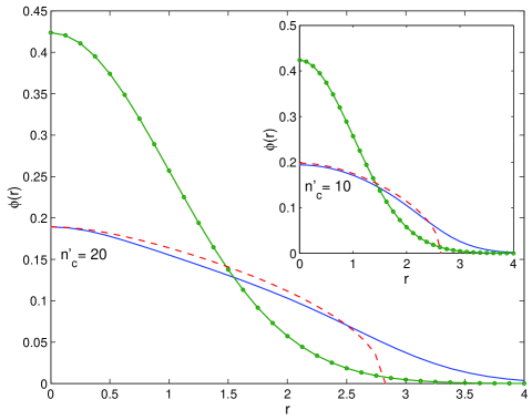
Figure 1: The profile of the ground state condensate wave function at $n^{\prime}_{c}=20$ and $n^{\prime}_{c}=10$ (solid line). The line with circle markers corresponds to the ideal Bose gas in an external harmonic confinement. Dashed line is for the density profile in the TF approximation (22).

The ground state density distribution $\rho_{0}({\bf r})$ is defined by the stationary equation ${\bf v}=0$, $\widetilde{\mu}=\mu_{B}$ and gives rise to the modified Gross- Pitaevskii equation

$$-\frac{\nabla^{2}\sqrt{\rho_{0}}}{2\sqrt{\rho_{0}}}+k_{0}\frac{r^{2}}{2}+\frac{u}{2}\rho_{0}+\frac{v}{2}\rho_{0}^{2}=\mu_{B}.$$ (20)

The condensate density $\rho({\bf r},t)$ is normalized to the number of atoms in the condensate $\int d^{3}r\rho({\bf r},t)=N$. In the $T\to 0$ limit, $N$ coincides with the total number of bosonic atoms in the trap.

Ground state properties of the mixture and numerical solutions of Eq. (20) have been considered in Ryzhov07 ; cr6 . It was shown that the TF approximation gives the good description of density distribution and BF mixture can be accurately considered in the TF approximation PRA06 . In TF approximation

$$k_{0}r^{2}-2\mu_{B}+u\rho_{0}+v\rho_{0}^{2}=0.$$ (21)

In this case the density profile has the form

$$\rho_{0}({\bf r})=\frac{n_{cr}}{R_{cr}}\left[R_{cr}-\sqrt{a^{2}+k_{0}r^{2}}\right],\quad r\leqslant R_{B},$$ (22)

where $n_{cr}=u/(2|v|)$, $R_{cr}^{2}=u^{2}/(4|v|)$, $R_{B}=R/\sqrt{k_{0}}$, $R^{2}=2\mu_{B}$, $a^{2}=R^{2}_{cr}-R^{2}$. In the limiting case of noninteracting Bose and Fermi clouds ($g_{BF}\to 0$, $v\to 0$, $a\gg 1$, $R_{cr}\approx a+R^{2}/2a$, $k_{0}\approx 1$, $n_{cr}/2R_{cr}=1/u$) we recover the TF distribution for single bose- condensate $\rho_{0}(r)=(R^{2}-r^{2})/u$.

The parameter $R$ up to a multiplicative factor $1/\sqrt{k_{0}}$ is the radius $R_{B}$ of the Bose condensate. In TF approximation Eq. (21) for the center of the trap enables to relate the value of $R$, i.e. $\mu$, with central density as $R^{2}=u\rho_{0}+v\rho_{0}^{2}$. Let us express $R$ through parameter $n^{\prime}_{c}$ as

$$R^{2}=n^{\prime}_{c}(1-\frac{|v|}{u^{2}}n^{\prime}_{c}).$$ (23)

The values of the parameter $R$ gains the maximal value $R=R_{cr}$ at $n^{\prime}_{c}=u^{2}/2|v|\approx 20$.

The numerical solution of Eq. (20) for the condensate wave function $\phi({\bf r})=\sqrt{\rho_{0}({\bf r})}$ and TF profile (22) are presented in Fig.  1. They parameterized by rescaled central density $n^{\prime}_{c}=un_{c}$, $n_{c}=|\phi(0)|^{2}$. Note that the wave functions in the figure are normalized to unity.

Figure 1 shows two characteristic profile of the condensate wave function with increasing the central density from $n^{\prime}_{c}=10$ to $n^{\prime}_{c}=20$. For $n^{\prime}_{c}\lesssim 20$, the behavior is characteristic of the Bose gas with repulsion, i.e. the evolution of the profile corresponds to a monotonic expansion of the boson cloud with increasing number of bosons. The cloud density becomes more flat at the trap center, approaching TF analytical solution. For $n^{\prime}_{c}\gtrsim 20$, the solution changes qualitatively: the central density begins to increase.

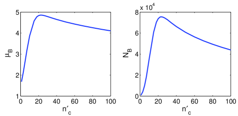
Figure 2: Chemical potential $\mu_{B}$ (in the unit of $\hbar\omega_{B}$) and number of bosons $N_{B}$ as functions of the rescaled central density $n^{\prime}_{c}$.

For $n^{\prime}_{c}\gtrsim 20$, the central density increases significantly in a small region near the trap center. We attribute the solution with $n^{\prime}_{c}\gtrsim 20$ to the nonstationary states of the condensate through which the collapse of the condensate wave function occurs. The value $n^{\prime}_{c}\approx 23$ corresponds the critical particle number $N_{Bc}\simeq 8\cdot 10^{4}$ above which collapse occurs. In that point the branch of stable solutions meets the branch of unstable solutions of the GP equation. This qualitative behavior is the generic signature of a Hamiltonian saddle node bifurcation Brachet99 .

Fig.  2 shows the boson chemical potential $\mu_{B}$ and the number of bosons $N_{B}$ as function of the parameter $n^{\prime}_{c}$, obtained at numerical solution of Eq. (20). Both curve have maximal value at $n^{\prime}_{c}\simeq 23$. The condition $\partial N/\partial n^{\prime}_{c}=0$ is a sufficient condition of the zero excitation mode Stoof96 . It means that it does not cost energy to deform the initial density profile continuously into the final, which indicates the threshold for instability

$$N(n^{\prime}_{c}+\delta n^{\prime}_{c})=\int{\>}d^{3}r{\,}\rho_{0}({\bf r},n^{\prime}_{c}+\delta n^{\prime}_{c})\simeq\\ \simeq\int{\>}d^{3}r{\,}\rho_{0}({\bf r},n^{\prime}_{c})=N(n^{\prime}_{c}).$$ (24)

It is interesting to note that the radius of the condensate $R_{B}=R/\sqrt{k_{0}}$ for TF function (23) qualitatively conform these behavior, i.e. it increases for $n^{\prime}_{c}<n^{\prime}_{c0}$ and decreases for $n^{\prime}_{c}>n^{\prime}_{c0}$. There is a critical point where the dependence $R_{B}(\mu_{B})$ shows the maximum. This remarkable feature indicates the onset of a collapse in the system Ryzhov07 . So we can anticipate some features in the dynamics of the bose- cloud near the collapse and in the eigenfrequency spectrum.

III.2 Collective excitation spectrum

We now give a brief overview of the calculation of the low- frequency collective mode spectrum. We have to give explicit solution of Eq. (19). The main difficulty associated with Eq. (19) is the proper treatment of the differential operator term ${\rm div}(\rho_{0}\nabla\delta\widetilde{\mu})$ with

$$\delta\widetilde{\mu}=-\frac{1}{2}\delta\left(\frac{1}{\sqrt{\rho}}{\>}\Delta\sqrt{\rho}\right)+\frac{u}{2}\delta\rho+v\rho\delta\rho_{0}.$$ (25)

For uniform Bose fluid with constant condensate density $\rho_{0}$ the first term accounting for quantum pressure reduces to $-1/(4\rho_{0})\Delta\delta\rho$ and the differential operator term is handled in the straightforward manner

$${\rm div}(\rho_{0}\nabla\delta\widetilde{\mu})=\rho_{0}{\>}\Delta\delta\widetilde{\mu}=-\frac{1}{4}{\,}\Delta^{2}\delta\rho+\frac{u\rho_{0}}{2}\Delta\delta\rho.$$ (26)

Eigenvalue modes are the plane waves $\delta\rho_{\bf q}({\bf r})=Ce^{i{\bf qr}}$ and the resulting eigenvalues are given by Lifshitz80 $\omega_{\bf q}^{2}=u\rho_{0}{\bf q}^{2}/2+{\bf q}^{4}/4$.

For an inhomogeneous Bose- condensate in a trap the TF approximation must be called on to describe analytically the condensate collective modes Stringari96 . For the ground state the TF density has the form

$$\rho_{0}(r)=\frac{R^{2}-r^{2}}{u},\qquad r\leqslant R,$$ (27)

where the radius of Bose- condensate is $R=2\mu_{B}$. In Eq. (25) one omits the quantum pressure term, $\delta\widetilde{\mu}\simeq u\delta\rho/2$, and

$${\rm div}(\rho_{0}\nabla\delta\widetilde{\mu})\simeq\frac{R^{2}-r^{2}}{2}\Delta\delta\rho+\nabla\left(\frac{R^{2}-r^{2}}{2}\right)\cdot\nabla\delta\rho$$ (28)

For a spherical trap, an eigenfunction of Eq. (19) can be written as a product $\delta\rho({\bf r})=\delta\rho_{nl}(r)Y_{lm}(\theta,\varphi)$ of the radial eigenfunction $\delta\rho_{nl}(r)$ and a spherical harmonic $Y_{lm}(\theta,\varphi)$, where $n$ is the radial quantum number. The associated eigenfunctions are polynomials of the form

$$\delta\rho_{nl}(r)=Cr^{l}w_{nl}(r^{2}/R^{2}){\>}\Theta(R-r),$$ (29)

where $\Theta(R-r)$ is the step function. The polynomials $w_{nl}(y)$ are polynomials of order $n$ and satisfy equation

$$y(1-y)w^{\prime\prime}+\left(\frac{2l+3}{2}-\frac{2l+5}{2}y\right)w^{\prime}-\frac{\epsilon-l}{2}w=0,$$ (30)

where $\epsilon=\omega^{2}$. They can be expressed through the hypergeometric function $w_{nl}(y)=F(\alpha,\beta,\gamma,y)$ with parameters $\alpha=n$, $\beta=l+3/2+n$, $\gamma=l+3/2$. The associated energy eigenvalues are found to be

$$\omega_{nl}^{2}=\omega_{B}^{2}(2n^{2}+l+n(2l+3)).$$ (31)

The hypergeometric function $F(\alpha,\beta,\gamma,y)$ satisfies the equation Abramowitz

$$y(1-y)F^{\prime\prime}+[\gamma-(\alpha+\beta+1)y]F^{\prime}-\alpha\beta F=0.$$ (32)

The eigenfunctions (29) for the Bose-condensed cloud fluctuations vanish outside the cloud radius $R$ and present a discontinuity at $R$. The discontinuity is physically acceptable in view of the fact that the kinetic energy term has been set as negligible in taking the strong- coupling limit.

Let us now address the issue in the case Bose- Fermi mixture. As well as in the previous case we omit the quantum pressure term in (25) and the perturbation for $\widetilde{\mu}$ takes the form

$$\delta\widetilde{\mu}=\frac{u}{2}\delta\rho+v\rho_{0}\delta\rho,\quad\nabla\delta\widetilde{\mu}=\left(\frac{u}{2}+v\rho_{0}\right)\nabla\delta\rho+v(\nabla\rho_{0})\delta\rho,$$ (33)

and

$${\rm div}(\rho_{0}\nabla\delta\widetilde{\mu})=\left(\frac{u}{2}\rho_{0}+v\rho_{0}^{2}\right)\Delta\delta\rho+\\ +\left(\frac{u}{2}\nabla\rho_{0}+\frac{3}{2}v\nabla\rho_{0}^{2}\right)\cdot\nabla\delta\rho+v\rho_{0}^{2}\left[\left(\frac{\nabla\rho_{0}}{\rho_{0}}\right)^{2}+\frac{\Delta\rho_{0}}{\rho_{0}}\right]\delta\rho.$$ (34)

Due to $\nabla\rho_{0}/\rho_{0}\ll 1$ we should omit the last two terms in square brackets in TF approximation. So we can rewrite the expression (34) in the form

$${\rm div}(\rho_{0}\nabla\delta\widetilde{\mu})\simeq\left(\frac{1}{2}(u\rho_{0}+v\rho_{0}^{2})+\frac{v}{2}\rho_{0}^{2}\right)\Delta\delta\rho+\\ +\nabla\left(\frac{1}{2}\left(u\rho_{0}+v\rho_{0}^{2}\right)+v\rho_{0}^{2}\right)\cdot\nabla\delta\rho.$$ (35)

Now we use in Eq. (35) the ground state density profile $\rho_{0}(\bf r)$ from Eq. (22), which simply states that due to Eq. (21) $u\rho_{0}+v\rho_{0}^{2}=2\mu_{B}-k_{0}r^{2}$ and come to the result

$${\rm div}(\rho_{0}\nabla\delta\widetilde{\mu})\simeq\left(\frac{R^{2}-k_{0}r^{2}}{2}+\frac{v\rho_{0}^{2}}{2}\right)\Delta\delta\rho+\\ +\nabla\left(\frac{R^{2}-k_{0}r^{2}}{2}+v\rho_{0}^{2}\right)\cdot\nabla\delta\rho.$$ (36)

Note that in the $v\to 0$ limit the Eq. (36) transforms into Eq. (28) for single Bose condensate. In principal, the solution of Eq. (19) with approximate ${\rm div}(\rho_{0}\nabla\delta\widetilde{\mu})$ giving by Eq. (36) should give rise to collective excitations spectra in TF approximation. But the term $v\rho_{0}^{2}$ is the complicated function with square root singularity. In order give analytical treatment of collective excitations we have to approximate the $v\rho_{0}^{2}$ term by more analytically simple function. It is reasonable to simplify the $v\rho_{0}^{2}$ term and approximate it by quadratic function on the radius $r$. For $\rho_{0}^{2}$ we use Eq. (22) and expand the radical near the center of the trap which gives rise to

$$\rho_{0}^{2}(r)\simeq\frac{1}{|v|}\frac{k_{0}b}{a}\left((R^{\prime}_{B})^{2}-r^{2}\right),$$ (37)

where $R^{\prime}_{B}=ab/k_{0}$ and $b=R_{cr}-a$. In the framework of the density profile (37) it is possible to give explicitly solutions of Eq. (19) through the hypergeometric functions.

It is clear that the result (37) does not describe density near $r=R^{\prime}_{B}$. This fact is an artifact of the TF approximation, arising from the vanishing of $\rho_{0}({\bf r})$ at $r=R^{\prime}_{B}$. The dependence $\rho_{0}^{2}$ in Eq. (37) has slightly different radius of the cloud $R^{\prime}_{B}$ in comparing with $R_{B}$ in Eq. (22), but this approximation is consistent with the TF approximation because in the region near boundary density of the cloud is small. Note that $(R^{\prime}_{B})^{2}=R^{2}/k_{0}-(R^{2}_{cr}-\sqrt{R_{cr}^{2}-R^{2}})/k_{0}$ and $R^{\prime}_{B}\simeq R_{B}$ at $R\ll R_{cr}$. In this regime the density profiles giving by Eqs. (22) and (37) are the similar. In contrast in the critical regime at $R\lesssim R_{cr}$ the parameter $R^{\prime}_{B}\ll R_{B}$ and the approximation Eq. (37) is no longer valid.

Now for $v\rho_{0}^{2}$ term in Eq. (36) we use expression (37) and introduce notations $\alpha_{1}=k_{0}(1-b/a)$, $\alpha_{2}=k_{0}(1-2b/a)$. Then

$${\rm div}(\rho_{0}\nabla\widetilde{\mu})=\frac{k_{0}R_{B}^{2}-\alpha_{1}r^{2}}{2}\Delta\delta\rho-\alpha_{2}r\frac{\partial}{\partial r}\delta\rho.$$ (38)

Now the equation (19) takes the form

$$\frac{R_{*}^{2}-r^{2}}{2}\Delta\delta\rho-\alpha_{3}r\frac{\partial}{\partial r}\delta\rho+\epsilon\delta\rho=0.$$ (39)

where $R_{*}^{2}=k_{0}R_{B}^{2}/\alpha_{1}$, $\alpha_{3}=\alpha_{2}/\alpha_{1}$, $\epsilon=\omega^{2}/\alpha_{1}$. Separating variables $\delta\rho({\bf r})=r^{l}{\,}G(r)Y_{lm}(\theta,\varphi)$ and substituting $y=r^{2}/R_{*}^{2}$, one obtains for the function $w(y)=G(r(y))$ the following equation:

$$y(1-y)w^{\prime\prime}+\left(\frac{2l+3}{2}-\frac{2l+3+2\alpha_{3}}{2}y\right)w^{\prime}+\frac{\epsilon-\alpha_{3}l}{2}w=0.$$ (40)

If we compare it with analogous Eq. (30) we can see that it contains additional parameters $\alpha_{1}$ and $\alpha_{2}$ including the effect of interparticle interaction. At $v\to 0$ the coefficients $\alpha_{1},\alpha_{2}\to 1$, and the Eq. (40) transforms into Eq. (30) for a pure boson system. Eq. (40) is a standard equation of the form (32) for hypergeometrical function $F(\alpha,\beta,\gamma,y)$. It should be a polynomial of $n$- th degree, which for $v\to 0$ tends to Stringari’s solution (29). So the parameters of the hypergeometrical function $F(\alpha,\beta,\gamma,y)$ get the values $\alpha=-n$, $\beta=(2l+1+2\alpha_{3})/2+n$, and $\gamma=(2l+3)/2$.

The associated energy eigenvalue are found to be (in dimensional units)

$$\omega_{nl}^{2}=\omega_{B}^{2}\left[\alpha_{1}(2n^{2}+n(2l+1))+\alpha_{2}(2n+l)\right].$$ (41)

The result (41) can be considered as a qualitative signature of shifts of eigenfrequencies in the presence of the boson- fermion coupling. At $v\to 0$ frequencies (41) transform into the Stringari’s spectrum (31).

The dispersion law of the normal modes given by the formula (41) has the additional coefficients $\alpha_{1}$ and $\alpha_{2}$ which incorporate the effect of interparticle interaction. In explicit form the coefficients $\alpha_{1}$ and $\alpha_{2}$ are related with $N_{B}$, $N_{F}$, and $g_{BF}$ through the parameters $R$ and $R_{cr}$

$$\alpha_{1}=k_{0}\left(1-\frac{R_{cr}-\sqrt{R_{cr}^{2}-R^{2}}}{\sqrt{R_{cr}^{2}-R^{2}}}\right)$$

$$\alpha_{2}=k_{0}\left(1-2\frac{R_{cr}-\sqrt{R_{cr}^{2}-R^{2}}}{\sqrt{R_{cr}^{2}-R^{2}}}\right)$$ (42)

Formally these relations are valid only at $R\ll R_{cr}$. In our approach we interpolate they up to $R\lesssim R_{cr}$. These rather crude approximation nevertheless gives rise to the qualitatively correct picture of collective excitation spectra tendency to become softening near the collapse transition.

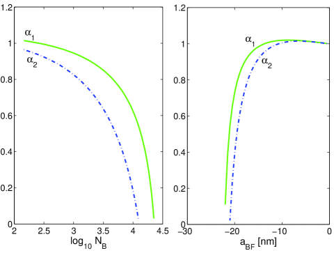
Figure 3: The coefficients $\alpha_{1}$ and $\alpha_{2}$ of the formula (41) as functions of $N_{B}$ and $|a_{BF}|$. Left panel: $u=0.11$, $v=-0.0003$. Right panel: $u=0.11$, $N_{B}=5\cdot 10^{3}$.

The coefficients $\alpha_{1}$ and $\alpha_{2}$ are plotted in Fig. 3 as functions of the number of bosons $N_{B}$ and scattering length $|a_{BF}|$. The chemical potential $\mu_{B}$, and the number of bosons $N_{B}$ are fixed by $N_{B}=\int\rho_{0}({\bf r})d^{3}r$. For small values of the $|a_{BF}|$ and $N_{B}$ the coefficients $\alpha_{1}$ and $\alpha_{2}$ approach to one, while for $N_{B}$ and $|a_{BF}|$ large enough, one observes, as expected, important deviations due to the boson- fermion interaction effects. The figure shows that the system will be in the collapse regime both at sufficiently large $|a_{BF}|$ and $N_{B}$.

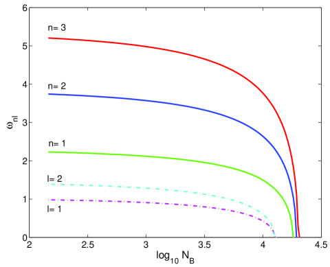
Figure 4: Frequencies $\omega_{nl}$ (in units $\omega_{B}$) of low- lying monopole modes $l=0$, $n=1,2,3$ (solid line), dipole and quadrupole modes $n=0$, $l=1,2$ (dashed-dotted line) as functions of the number of boson atoms $N_{B}$.

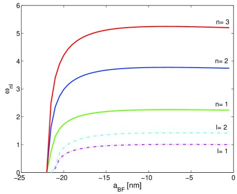
Figure 5: Frequencies $\omega_{nl}$ (in units $\omega_{B}$) of low-lying monopole modes $l=0$, $n=1,2,3$ (solid line), dipole and quadrupole modes ($n=0$, $l=1,2$) (dashed-dotted line) as functions of the scattering length $a_{BF}$ for $N_{B}=5\cdot 10^{3}$.

We will further limit the discussion to the case of excitations of low multipolarity corresponding to the energy range $\omega_{nl}\lesssim\mu$, where prediction (41) is expected to be accurate. To illustrate the dependence (41) we consider the low-lying monopole modes ($l=0$) and the surface excitation modes ($n=0$), and keep the number of fermions fixed.

In Fig. 4 we show the evolution of $\omega_{nl}$ as a function of number of bosons for $a_{BF}=-21.7$ nm. Three low- lying monopole modes corresponding $n=1,2,3$ and dipole and quadrupole modes are shown. At increasing values of the boson number the frequencies of modes display a monotonic decrease and ultimately vanish in the vicinity of the collapse. Points of a collapse are slightly different for different modes. This is a result of a rather crude approximation that we chose for the equilibrium density $\rho_{0}({\bf r})$. The second source of errors comes from the TF approximation. Results based on the TF approximation are in fact not adequate in the vicinity of $r\simeq R_{B}$ and beyond. If one works with the full hydrodynamic theory keeping the kinetic energy contributions in (19), one finds that $\rho_{0}({\bf r})$ does not abruptly vanish at $r=R_{B}$ but exhibits a small tail which slowly goes to zero. This tail is neglected in our approximation. Nevertheless the behavior correctly display the situation which occurs near the collapse. The similar frequency behavior of the bosonic modes as a signature of the incipient collapse has been obtained Capuzzi et al. with numerical calculations on the basis of generalized hydrodynamics equations Capuzzi04 .

Fig. 5 shows the frequencies $\omega$ of the same low- lying monopole and surface modes as in Fig. 4 as functions of the scattering length $a_{BF}$ at fixed number of bosons $N_{B}=5\cdot 10^{3}$. At larger values of $|a_{BF}|$ the eigenfrequencies show softening as collapse is approached. In contrast with the previous picture the points of the collapse are approximately the same for different modes. At increasingly large boson- fermion attraction the densities of the two species increase in their overlap region and collapse occurs when this attraction overcomes the Fermi kinetic pressure and the boson- boson repulsion. Similar behavior has been revealed in ⁷Li-⁶Li mixture with numerical calculation of eigenfrequencies Capuzzi04 .

Note that both components of the ⁸⁷Rb-⁴⁰K mixture are inside the same magnetic trap, but their trapping frequencies differ considerably as a consequence of the large difference in atomic masses. At this conditions the generalized Kohn theorem Dobson94 is satisfied when the species are uncoupled ($a_{BF}\to 0$) and each component enable to oscillate with its own frequency. From Fig.  5 one can see that the dipole mode frequency $\omega_{D}$ ($n=0,l=1$) in broad region on $a_{BF}$ except near the collapse regime is found to be not affected by the interactions and equals to the confining potential frequency $\omega_{B}$. In fact this mode corresponds to the oscillation of the center of mass of the Bose- gas with $\omega_{D}=\omega_{B}$ driven by the external harmonic potentials. The same one can say on the monopole $\omega_{M}$ and the quadrupole $\omega_{Q}$ mode frequencies. In this limit ($a_{BF}\to 0$) one recovers the results $\omega_{M}=\sqrt{5}\omega_{B}$ ($n=1,l=0$) and $\omega_{Q}=\sqrt{2}\omega_{B}$ ($n=0,l=2$) predicted by the hydrodynamic theory of superfluid Stringari96 .

In Ref. Miyakawa2000 ; Sogo02 the collective oscillations were calculated by the sum-rule approach and collisionless random-phase approximation (RPA). Mixing angle of bosonic and fermionic multipole operators was introduced so that the mixing characters of the low- lying collective modes were studied as functions of the boson- fermion interaction strength. For an attractive boson- fermion interaction it was shown that the low-lying monopole mode becomes a coherent oscillation of bosons and fermions and shows a rapid decrease in the excitation energy towards the instability point of the ground state. In contrast, the quadrupole mode give indications of frequency increasing and it contradicts the behavior of modes in Ref. Capuzzi04 . In Ref. Capuzzi04 instead it was found that, as the mixture is driven towards collapse instability, the frequencies of the modes of bosonic origin show a softening, which becomes most pronounced in the very proximity of collapse. Explicit illustrations of these trends were given for the monopolar spectra.

A comparison of the hydrodynamic spectra Capuzzi04 with the spectra calculated on the basis of the effective Hamiltonian suggests that eigenvalue equations with the dynamical coupling between the two components yield the similar bosonic mode behavior both as functions of $N_{B}$ and $a_{BF}$ as the hydrodynamic- type equations (19) with the fermion degree of freedom being integrated out. Softening of the bosonic mode spectrum is a general signature of the dynamics of the Bose- Fermi mixture with attraction between components arising from peculiar properties of the ground state and instability point near the collapse transition.

IV Summary

We have studied the collective mode frequencies in the boson- fermion mixture. To this purpose we have used the effective Hamiltonian for the Bose system, where the fermion degrees of freedom are integrated out ChRyz04 ; cr5 . The effective Hamiltonian incorporates the three- particle elastic collisions induced by the boson- fermion interaction. In terms of coupled eigenvalue density fluctuation equations for the bosonic and fermionic components it means that we exclude fermion fluctuations from the bosonic density fluctuation component resulting in more involved structure of bosonic fluctuations.

This approach enables to account for interparticle interaction strength in collective excitation frequencies and can be considered as an extension of Stringari’s solution Stringari96 for Bose - Fermi mixtures. The analysis of the mode frequencies as function of the number of boson atoms and the boson- fermion coupling strength yields a dynamical condition for a collapse of the system. The behavior of mode frequencies is consistent with numerical analysis on the basis of generalized hydrodynamics equations Capuzzi04 . The effective Hamiltonian approach proves to be efficient tool for the analysis of both the ground state and dynamical properties of boson- fermion mixtures and can be considered as alternatives to Capuzzi’s et al. Capuzzi04 approach for analysis boson eigenfrequencies. We also note that the present study can be extended to take into account finite temperature effect Ryzhov08 on the excitations.

V Acknowledgement

The work was supported by CRDF (A.M.B.) [Grant No. BF4M11] and the Russian Foundation for Basic Research (V.N.R)(Grants No 08-02-00781 and No 10-02-00700), and Russian Federal Program 02.740.11.5160.

References

- (1) M. N. Anderson, J. R. Ensher, M. R. Matthews et al., Science 269, 198 (1995).
- (2) K. B. Davis, M.-O. Mewes, M. R. Andrews et al., Phys. Rev. Lett. 75, 3969 (1995).
- (3) C. C. Bradley, C. A. Sackett, and R. G. Hulet, Phys. Rev. Lett. 78, 985 (1997).
- (4) I. Bloch, J. Dalibard, and W. Zwerger, Rev. Mod. Phys. 80, 885 (2008).
- (5) S. Giorgini, L. P. Pitaevskii, and S. Stringari, Rev. Mod. Phys. 80, 1215 (2008).
- (6) S. T. Chui, V. N. Ryzhov, and E. E. Tareyeva, JETP 91,1183(2000).
- (7) S. T. Chui, V. N. Ryzhov, and E. E. Tareyeva, Phys. Rev. A 63, 023605 (2001).
- (8) S. T. Chui, V. N. Ryzhov, and E. E. Tareyeva, J. Phys.: Condensed Matter 14, L77 (2002).
- (9) S. T. Chui, V. N. Ryzhov, and E. E. Tareyeva, Jetp Letters, 75, 233 (2002).
- (10) B. DeMarco and D. S. Jin, Science 285, 1703 (1999).
- (11) A. G. Truscott, K. E. Strecker, W. I. McAlexander et al, Science 291, 2570 (2001).
- (12) F. Schreck, L. Khaykovich, K. L. Corwin et al, Phys. Rev. Lett. 87, 080403 (2001).
- (13) Z. Hadzibabic, C. A. Stan, K. Dieckmann et al, Phys. Rev. Lett. 88, 160401 (2002).
- (14) G. Modungo, G. Roati, F. Riboli et al, Science 297, 2240 (2002).
- (15) J. Goldwin, S. B. Papp, B. DeMarco, and D. S. Jin, Phys. Rev. A 65, 021402(R) (2002).
- (16) N. Nygaard and K. Molmer, Phys. Rev. A 59, 2974 (1999).
- (17) X.X. Yi and C.P. Sun, Phys. Rev. A 64, 043608 (2001).
- (18) A. Minguzzi and M.P. Tosi, Phys. Lett. A 268, 142 (2000).
- (19) Z. Akdeniz, A. Minguzzi, P. Vignolo and M.P. Tosi, Phys. Rev. A 66, 013620 (2002).
- (20) P. Capuzzi and E.S. Hernandez, Phys. Rev. A 66, 035602 (2002);
- (21) R. Roth and H. Feldmeier, Phys. Rev. A 65, 021603(R) (2002); R. Roth, ibid. 66, 013614 (2002).
- (22) K. Molmer, Phys. Rev. Lett. 80, 1804 (1998).
- (23) D.M. Jezek, M. Barranco, M. Guilleumas, R. Mayol, and M. Pi, Phys. Rev. A 70, 043630 (2004).
- (24) M.J. Bijlsma, B.A. Heringa, and H.T.C. Stoof, Phys. Rev. A 61, 053601 (2000).
- (25) C. Ospelkaus, S. Ospelkaus, K. Sengstock, and K. Bongs, Phys. Rev. Lett. 96, 020401 (2006).
- (26) P. Capuzzi and E.S. Hernandez, Phys. Rev. A 64, 043607 (2001); J. Low Temp. Phys. 126, 425 (2002).
- (27) T. Maruyama, H. Yabu, and T. Suzuki, Phys. Rev. A 72, 013609 (2005).
- (28) P. Capuzzi, A. Minguzzi, and M.P. Tosi, Phys. Rev. A 67, 053605 (2003).
- (29) P. Capuzzi, A. Minguzzi, and M.P. Tosi, Phys. Rev. A 68, 033605 (2003).
- (30) P. Capuzzi, A. Minguzzi, and M.P. Tosi, Phys. Rev. A 69, 053615 (2004).
- (31) T. Miyakawa, T. Suzuki, and H. Yabu, Phys. Rev. A 62, 063613 (2000).
- (32) T. Sogo, T. Miyakawa, T. Suzuki, and H. Yabu, Phys. Rev. A 66, 013618 (2002).
- (33) S. Stringari, Phys. Rev. Lett. 77, 2360 (1996).
- (34) M. Edwards, P. A. Ruprecht, K. Burnett, R. J. Dodd and C. W. Clark, Phys. Rev. Lett. 77, 1671 (1996).
- (35) M. Ueda and A. Leggett, Phys. Rev. Lett. 80, 1576 (1998).
- (36) S. T. Chui and V. N. Ryzhov, Phys. Rev. A 69, 043607 (2004).
- (37) S. T. Chui, V. N. Ryzhov, and E. E. Tareyeva, JETP Lett. 80, 274 (2004).
- (38) V. N. Popov, Functional Integrals in Quantum Field Theory and Statistical Physics (Reidel, Dordrecht, 1983).
- (39) H. T. C. Stoof, in Proceedings of the Les Houches Summer School on Coherent Atomic Matter Waves, Session LXXII, 1999, Ed. by R. Kaiser, C. Westbrook, and F. David (Springer, Berlin, 2001), pp. 219-316; e-print arXiv: cond-matt/9910441.
- (40) F. Dalfovo, S. Giorgini, L. P. Pitaevskii, and S. Stringari, Rev. Mod. Phys. 71, 463 (1999).
- (41) Yu. Kagan, G. V. Shlyapnikov, and J. T. M. Walraven, Phys. Rev. Lett. 76, 2670 (1996); Yu. Kagan, A. E. Muryshev, and G. V. Shlyapnikov, ibid. 81, 933 (1998).
- (42) A.L. Fetter, Phys. Rev. A 53, 4245 (1996).
- (43) D. A. Butts and D. S. Rokhsar, Phys. Rev. A 55, 4346 (1997).
- (44) A.M. Belemuk, V.N. Ryzhov, and S.-T. Chui, Phys. Rev. A 76, 013609 (2007).
- (45) A. M. Belemuk, V. N. Ryzhov, and S.-T. Chui, JETP Lett. 84, 294 (2006).
- (46) A.M. Belemuk, N.M. Chtchelkatchev, V.N. Ryzhov, and S.-T. Chui, Phys. Rev. A 73, 053608 (2006).
- (47) C. Huepe, S. Metens, G. Dewel, P. Borckmans, and M.E. Brachet, Phys. Rev. Lett. 82, 1616 (1999).
- (48) M. Houbiers and H.T.C. Stoof, Phys. Rev. A 54, 5055 (1996).
- (49) J.F. Dobson, Phys. Rev. Lett. 73, 2244 (1994).
- (50) A.M. Belemuk and V.N. Ryzhov, JETP Lett. 87, 376 (2008)
- (51) E. M. Lifshitz and L. P. Pitaevskii, Statistical Physics, Part 2 (Pergamon Press, Oxford, 1980).
- (52) Handbook of Mathematical Functions with Formulas, Graphs, and Mathematical Tables, edited by M. Abramowitz and I.A. Stegun, Natl. Bur. Stand. Appl. Math. Ser. No. 55 (U.S. GPO, Washington, DC, 1968), Chaps. 15 and 22.