On Graphs and Codes Preserved by
Edge Local Complementation

Abstract

Orbits of graphs under local complementation (LC) and edge local complementation (ELC) have been studied in several different contexts. For instance, there are connections between orbits of graphs and error-correcting codes. We define a new graph class, ELC-preserved graphs, comprising all graphs that have an ELC orbit of size one. Through an exhaustive search, we find all ELC-preserved graphs of order up to 12 and all ELC-preserved bipartite graphs of order up to 16. We provide general recursive constructions for infinite families of ELC-preserved graphs, and show that all known ELC-preserved graphs arise from these constructions or can be obtained from Hamming codes. We also prove that certain pairs of ELC-preserved graphs are LC equivalent. We define ELC-preserved codes as binary linear codes corresponding to bipartite ELC-preserved graphs, and study the parameters of such codes.

1 Introduction

The local complementation (LC) operation was first defined by Kotzig [26] and later studied by de Fraysseix [15], Fon-der-Flaas [17], and Bouchet [7]. Bouchet also introduced edge local complementation (ELC) [7], an operation which is also known as pivoting on a graph. LC orbits of graphs have been used to study quantum graph states [20, 31], which are equivalent to self-dual additive codes over $\mathbb{F}_{4}$ [10]. LC orbits have been used to classify such codes [12]. There are also connections between graph orbits and properties of Boolean functions [29, 30]. Interlace polynomials of graphs have been defined with respect to both LC [1] and ELC [3]. These polynomials encode certain properties of the graph orbits, and were originally used to study a problem related to DNA sequencing [2]. Connections between interlace polynomials and error-correcting codes have also been studied [14]. Bouchet [8] proved that a graph is a circle graph if and only if certain induced subgraphs, or obstructions, do not appear anywhere in its LC orbit. Similarly, circle graph obstructions under ELC were described by Geelen and Oum [18].

In this paper, we introduce ELC-preserved graphs as a new class of graphs, namely those that are invariant under the ELC operation and therefore having trivial ELC orbits of size one. In light of the previous works and various applications listed in the previous paragraph, we feel that ELC-preserved graphs are fundamental objects worthy of study and, for this paper, we consider both graph- and code-theoretic interpretations of these objects.

Bipartite graphs correspond to binary linear error-correcting codes. ELC can be used to generate orbits of equivalent codes and has previously been used to classify codes [13]. It has also been shown that ELC can improve the performance of iterative decoding [25, 22, 24, 23]. ELC-preserved graphs are of particularly interest in this context, since for such graphs the decoding algorithm is equivalent to a variant of permutation decoding [25, 19].

We will show that the class of codes corresponding to bipartite ELC-preserved graphs, which we will call ELC-preserved codes, is a superset of both the Hamming codes and the extended Hamming codes, which makes it an interesting class of codes. When it comes to practical applications in iterative decoding, we conclude that the ELC-preserved criterion might be too strict to obtain good codes with appropriate length. However, we suggest that ELC-preserved graphs could be a building block for good codes, and when we look at “almost ELC-preserved” graphs with ELC-orbits of size two, we find both the Golay code and a BCH code. Other relaxations of the ELC-preserved criterion yielding practical error-correction applications have been considered in other works [25, 24]. In this paper we focus on the theoretical properties of ELC-preserved graphs and codes.

This paper is organized as follows. Section 2 introduces all necessary notation from graph theory and coding theory. In Section 3, we show that there do exist non-trivial bipartite and non-bipartite ELC-preserved graphs. We find all ELC-preserved graphs of order up to 12 and all ELC-preserved bipartite graphs of order up to 16. In Section 4, we show that star graphs and complete graphs as well as graphs corresponding to Hamming codes and extended Hamming codes are ELC-preserved. We then prove that more ELC-preserved graphs can be obtained from four recursive constructions. Given a bipartite ELC-preserved graph, a larger bipartite ELC-preserved graph is constructed by star expansion. Similarly, clique expansion produces non-bipartite ELC-preserved graphs. Hamming expansion and the related Hamming clique expansion use a special graph of order seven, corresponding to a Hamming code, to obtain new ELC-preserved graphs. In Section 5, we show that all ELC-preserved graphs of order up to 12, and all ELC-preserved bipartite graphs of order up to 16, are obtained from these constructions. We also prove that certain pairs of ELC-preserved graphs are LC equivalent. In particular, from extended Hamming codes, we obtain new non-bipartite ELC-preserved graphs via LC. The properties of ELC-preserved codes obtained from star expansion and Hamming expansion are described in Section 6. In particular, we enumerate and construct new self-dual ELC-preserved codes. In Section 7 we briefly consider the generalization from ELC-preserved graphs to graphs with orbits of size two, and study the corresponding codes. Finally, in Section 8, we conclude with some ideas for future research.

2 Preliminaries

2.1 Graphs

A graph is a pair $G=(V,E)$ where $V$ is a set of vertices, and $E\subseteq V\times V$ is a set of edges. The order of $G$ is $n=|V|$. A graph of order $n$ can be represented by an $n\times n$ adjacency matrix $\Gamma$, where $\Gamma_{i,j}=1$ if $\{i,j\}\in E$, and $\Gamma_{i,j}=0$ otherwise. We will only consider simple undirected graphs, whose adjacency matrices are symmetric with all diagonal elements being 0, i.e., all edges are bidirectional and no vertex can be adjacent to itself. The neighborhood of $v\in V$, denoted $N_{v}\subset V$, is the set of vertices connected to $v$ by an edge. The number of vertices adjacent to $v$ is called the degree of $v$. The induced subgraph of $G$ on $W\subseteq V$ is the graph that has $W$ as a set of vertices and has all edges in $E$ whose endpoints are both in $W$. The complement of $G$ is a graph with the same vertex set, $V$, but whose edge set consists of the edges not present in G, i.e., the complement of $E$. (Note that the complement will also be a simple graph, i.e., no loops are introduced.) Two graphs $G=(V,E)$ and $G^{\prime}=(V,E^{\prime})$ are isomorphic if and only if there exists a permutation $\pi$ on $V$ such that $\{u,v\}\in E$ if and only if $\{\pi(u),\pi(v)\}\in E^{\prime}$. A path is a sequence of distinct vertices, $(v_{1},v_{2},\ldots,v_{i})$, such that $\{v_{1},v_{2}\},\{v_{2},v_{3}\},$ $\ldots,\{v_{i-1},v_{i}\}\in E$. A graph is connected if there is a path from any vertex to any other vertex in the graph. A graph is bipartite if its set of vertices can be decomposed into two disjoint sets, called partitions, such that no two vertices within the same set are adjacent, and non-bipartite otherwise. We call a graph $(a,b)$-bipartite if these partitions are of size $a$ and $b$, respectively.

Definition 1 ( [17, 7, 15]).

Given a graph $G=(V,E)$ and a vertex $v\in V$, let $N_{v}\subset V$ be the neighborhood of $v$. Local complementation (LC) on $v$ transforms $G$ into $G*v$ by replacing the induced subgraph of $G$ on $N_{v}$ by its complement. (For an example, see Fig. 1)

(a) The graph $G$

(b) The graph $G*1$

Fig. 1: Example of local complementation

Definition 2 ( [7]).

Given a graph $G=(V,E)$ and an edge $\{u,v\}\in E$, edge local complementation (ELC) on $\{u,v\}$ transforms $G$ into $G^{(u,v)}=G*u*v*u=G*v*u*v$.

Definition 3 ( [7]).

ELC on $\{u,v\}$ can equivalently be defined as follows. Decompose $V\setminus\{u,v\}$ into the following four disjoint sets, as visualized in Fig. 2.

1. Vertices adjacent to $u$, but not to $v$.

2. Vertices adjacent to $v$, but not to $u$.

3. Vertices adjacent to both $u$ and $v$.

4. Vertices adjacent to neither $u$ nor $v$.

To obtain $G^{(u,v)}$, perform the following procedure. For any pair of vertices $\{x,y\}$, where $x$ belongs to class $A$, $B$, or $C$, and $y$ belongs to a different class $A$, $B$, or $C$, “toggle” the pair $\{x,y\}$, i.e., if $\{x,y\}\in E$, delete the edge, and if $\{x,y\}\not\in E$, add the edge $\{x,y\}$ to $E$. Finally, swap the labels of vertices $u$ and $v$.

Fig. 2: Visualization of the ELC operation

Definition 4.

The graphs $G$ and $G^{\prime}$ are LC-equivalent (resp. ELC-equivalent) if a graph isomorphic to $G^{\prime}$ can be obtained by applying a finite sequence of LC (resp. ELC) operations to $G$. The LC orbit (resp. ELC orbit) of $G$ is the set of all non-isomorphic graphs that can be obtained by performing any finite sequence of LC (resp. ELC) operations on $G$.

For bipartite graphs, we can simplify the ELC operation, since the set $C$ in Definition 3 must be empty. Given a bipartite graph $G=(V,E)$ and an edge $\{u,v\}\in E$, $G^{(u,v)}$ can be obtained by “toggling” all edges between the sets $N_{u}\setminus\{v\}$ and $N_{v}\setminus\{u\}$, followed by a swapping of vertices $u$ and $v$. Moreover, if $G$ is an $(a,b)$-bipartite graph, then, for any edge $\{u,v\}\in E$, $G^{(u,v)}$ must also be $(a,b)$-bipartite [29]. Note that LC does not, in general, preserve bipartiteness. It follows from Definition 2 that every LC orbit can be partitioned into one or more ELC orbits. If $G=(V,E)$ is a connected graph, then, for any vertex $v\in V$, $G*v$ must also be connected. Likewise, for any edge $\{u,v\}\in E$, $G^{(u,v)}$ must be connected.

Definition 5.

A graph $G$ is ELC-preserved if for any edge $\{u,v\}\in E$, $G^{(u,v)}$ is isomorphic to $G$. In other words, $G$ is ELC-preserved if and only if the ELC orbit has $G$ as the only element.

We only consider connected graphs, since a disconnected graph is ELC-preserved if and only if its connected components are ELC-preserved. Trivially, empty graphs, i.e., graphs with no edges, are ELC-preserved.

2.2 Codes

A binary linear code, $\mathcal{C}$, is a linear subspace of $\mathbb{F}_{2}^{n}$ of dimension $k$. The $2^{k}$ elements of $\mathcal{C}$ are called codewords. The Hamming weight of a codeword is the number of non-zero components. The minimum distance of $\mathcal{C}$ is equal to the smallest non-zero weight of any codeword in $\mathcal{C}$. A code with minimum distance $d$ is called an $[n,k,d]$ code. Two codes are equivalent if one can be obtained from the other by a permutation of the coordinates. A permutation that maps a code to itself is called an automorphism. All automorphisms of $\mathcal{C}$ make up its automorphism group. We define the dual code of $\mathcal{C}$ with respect to the standard inner product, $\mathcal{C}^{\perp}=\{\boldsymbol{u}\in\mathbb{F}_{2}^{n}\mid\boldsymbol{u}\cdot\boldsymbol{c}=0\text{ for all }\boldsymbol{c}\in\mathcal{C}\}$. $\mathcal{C}$ is called self-dual if $\mathcal{C}=\mathcal{C}^{\perp}$, and isodual if $\mathcal{C}$ is equivalent to $\mathcal{C}^{\perp}$. The code $\mathcal{C}$ can be defined by a $k\times n$ generator matrix, $C$, whose rows span $\mathcal{C}$. By column permutations and elementary row operations $C$ can be transformed into a matrix of the form $C^{\prime}=(I\mid P)$, where $I$ is a $k\times k$ identity matrix, and $P$ is some $k\times(n-k)$ matrix. The matrix $C^{\prime}$, which is said to be of standard form, generates a code which is equivalent to $\mathcal{C}$. The matrix $H^{\prime}=(P^{\text{T}}\mid I)$, where $I$ is an $(n-k)\times(n-k)$ identity matrix is the generator matrix of $\mathcal{C}^{\prime\perp}$ and is called the parity check matrix of $\mathcal{C}^{\prime}$.

Definition 6 ( [11, 27]).

Let $\mathcal{C}$ be a binary linear $[n,k]$ code with generator matrix $C=(I\mid P)$. Then the code $\mathcal{C}$ corresponds to the $(k,n-k)$-bipartite graph on $n$ vertices with adjacency matrix

$$\Gamma=\begin{pmatrix}\boldsymbol{0}_{k\times k}&P\\ P^{\text{T}}&\boldsymbol{0}_{(n-k)\times(n-k)}\end{pmatrix},$$

where $\boldsymbol{0}$ denotes all-zero matrices of the specified dimensions.

Theorem 1 ( [13]).

Applying any sequence of ELC operations to a graph corresponding to a code $\mathcal{C}$ will produce another graph corresponding to the code $\mathcal{C}$. Moreover, graphs corresponding to equivalent codes will always belong to the same ELC orbit (up to isomorphism).

Note that, up to isomorphism, one bipartite graph corresponds to both the code $\mathcal{C}$ generated by $(I\mid P)$, and the code $\mathcal{C}^{\perp}$ generated by $(P^{\text{T}}\mid I)$. When $\mathcal{C}$ is isodual, the ELC-orbit of the associated graph corresponds to a single equivalence class of codes. Otherwise, the ELC-orbit corresponds to two equivalence classes, that of $\mathcal{C}$ and that of $\mathcal{C}^{\perp}$ [13].

Definition 7.

An ELC-preserved code is a binary linear code corresponding to an ELC-preserved bipartite graph.

It follows from Theorem 1 that ELC allows us to jump between all standard form generator matrices of a code. Hence an ELC-preserved code is a code that has only one standard form generator matrix, up to column permutations.

Theorem 2 ( [13]).

The minimum distance of an $[n,k,d]$ binary linear code $\mathcal{C}$ is $d=\delta+1$, where $\delta$ is the smallest vertex degree of any vertex in a fixed partition of size $k$ over all graphs in the associated ELC orbit. The minimum vertex degree in the other partition over the ELC orbit gives the minimum distance of $\mathcal{C}^{\perp}$.

For an ELC-preserved graph, Theorem 2 means that the minimum distance of the associated code, and its dual code, can be found simply by finding the minimum vertex degree in each partition of the graph.

In the technique of iterative decoding with ELC [25, 22, 24, 23], labeled graphs are used, so that ELC is equivalent to row additions on an initial generator matrix of the form $(I\mid P)$, which means that the corresponding code is preserved. (It is the parity check matrix of the code that is actually used for decoding, but we have already seen that, up to isomorphism, the bipartite graph corresponding to the generator matrix and parity check matrix of a code is the same.) For an ELC-preserved code, all generator matrices must be column permutations of one unique generator matrix, and hence these permutations must all be automorphisms of the code. It follows that iterative decoding with ELC on an ELC-preserved code is equivalent to a variant of permutation decoding [25, 19].

3 Enumeration

From previous classifications [12, 13], we know the ELC orbit size for all graphs of order $n\leq 12$, and all bipartite graphs of order $n\leq 15$. (A database of ELC orbits is available on-line at http://www.ii.uib.no/~larsed/pivot/.) We find that a small number of ELC orbits of size one exist for each order $n$. Despite the much smaller number of bipartite graphs, there are approximately the same number of ELC-preserved bipartite and non-bipartite graphs for $n\leq 12$. The numbers of ELC-preserved graphs, together with the total numbers of ELC orbits, are given in Table 1. Note that all numbers are for connected graphs.

By using an extension technique we were also able to generate all ELC-preserved bipartite graphs of order $n=16$. Given the 1,156,716 ELC orbit representatives for $n=15$, we extend each $(a,b)$-bipartite graph in $2^{a}+2^{b}-2$ ways, by adding a new vertex and connecting it to all possible combinations of at least one of the old vertices. The complete set of extended graphs is significantly smaller than that set of all bipartite connected graphs of order 16, but it must contain at least one representative from each ELC orbit. To see that this is true, consider a connected bipartite graph $G$ of order 16. The induced subgraph on any 15 vertices of $G$ must be ELC-equivalent to one of the graphs that were extended to form the extended set, and hence there must be at least one graph in the extended set that is ELC-equivalent to $G$. We check each member of the extended set, and find that there are 6 connected bipartite ELC-preserved graphs of order 16. Note that this is the same extension technique that was used to classify ELC orbits [13], but checking if a graph is ELC-preserved is much faster than generating its entire ELC orbit, since we only need to consider ELC on each edge of the graph, and can stop and reject the graph as soon as a second orbit member is discovered.

Table 1: Number of non-bipartite ELC orbits ($nb_{n}$), non-bipartite ELC-preserved graphs ($nbp_{n}$), bipartite ELC orbits ($b_{n}$), and bipartite ELC-preserved graphs ($bp_{n}$)

$n$	$nb_{n}$	$nbp_{n}$	$b_{n}$	$bp_{n}$
2	-	-	1	1
3	1	1	1	1
4	2	1	2	1
5	7	1	3	1
6	27	2	8	2
7	119	1	15	2
8	734	2	43	3
9	6,592	3	110	2
10	104,455	3	370	2
11	3,369,057	2	1,260	1
12	231,551,924	6	5,366	5
13			25,684	1
14			154,104	5
15			1,156,716	4
16			?	6

4 Constructions

For all $n\geq 2$, there is a bipartite ELC-preserved graph of order $n$, namely the star graph, denoted $s^{n}$. This graph has one vertex, $v$, of degree $n-1$ and $n-1$ vertices, $u_{1},u_{2},\ldots,u_{n-1}$, of degree 1. Clearly the graph is ELC-preserved, since for all edges $\{u_{i},v\}$, $N_{u_{i}}\setminus\{v\}=\emptyset$. The construction given in Theorem 3 gives us more bipartite ELC-preserved graphs. For brevity, we will denote $N_{v}^{u}=N_{v}\setminus(N_{u}\cup\{u\})$. Let $e^{n}$ denote the empty graph on $n$ vertices, i.e., a graph with no edges.

Definition 8 ( [6, 3]).

Given a graph $G=(V,E)$, a vertex $v\in V$, and another graph $H=(V^{\prime},E^{\prime})$, where $V\cap V^{\prime}=\emptyset$, by substituting $v$ with $H$, we obtain the graph $G^{\prime}=((V\setminus\{v\})\cup V^{\prime},E^{\prime\prime})$, where $E^{\prime\prime}$ is obtained by taking the union of $E$ and $E^{\prime}$, removing all edges incident on $v$, and joining all vertices in $V^{\prime}$ to $w$ whenever $\{v,w\}\in E$.

Definition 9 ( [16]).

Given a graph $G=(V,E)$, and a vertex $v\in V$, we add a pendant at $v$ by adding a new vertex $w$ to $V$ and a new edge $\{v,w\}$ to $E$.

Theorem 3 (Star expansion).

Given an ELC-preserved bipartite graph $G=(V,E)$ on $k$ vertices and an integer $m>1$, we obtain an ELC-preserved bipartite graph $S^{m}(G)$ on $n=km$ vertices by substituting all vertices in one partition of $G$ with $e^{m}$ and adding $m-1$ pendants to all vertices in the other partition.

Proof.

Let $\{u,v\}\in E$. Without loss of generality, assume that $u$ is substituted by $u_{1},\ldots,u_{m}$, all incident on $v$. Moreover, pendant vertices $w_{1},\ldots,w_{m-1}$ are added, with $v$ as their only neighbor. Clearly ELC on $\{v,w_{i}\}$ is ELC-preserving. Due to symmetries, it only remains to show that ELC on an edge $\{u_{i},v\}$ preserves $S^{m}(G)$. In the graph $G$, let $A=N_{u}^{v}$ and $B=N_{v}^{u}$. In the graph $S^{m}(G)$, $N_{u_{i}}^{v}=A$, and $N_{v}^{u_{i}}=(B_{1}\cup\cdots\cup B_{m})\cup C\cup D$, where $C=\{w_{1},\ldots,w_{m-1}\}$ and $D=\{u_{1},\ldots,u_{m}\}\setminus\{u_{i}\}$. The subgraph induced on $A\cup B_{j}$ in $S^{m}(G)$, for $1\leq j\leq m$, is isomorphic to the subgraph induced on $A\cup B$ in $G$. ELC on $\{u_{i},v\}$ means that we toggle all pairs of vertices between $N_{u_{i}}^{v}$ and $N_{v}^{u_{i}}$. Toggling pairs between $A$ and $B_{j}$, for $1\leq j\leq m$, preserves $S^{m}(G)$, since toggling pairs between $A$ and $B$ preserves $G$. (The fact that all vertices in $A$ have $m-1$ added pendants has no effect on this.) Finally, in addition to swapping $u_{i}$ and $v$, ELC has the effect of toggling pairs of vertices between $A$ and $C$, and between $A$ and $D$. In $S^{m}(G)$, all vertices in $A$ are connected to all vertices in $D$, and no vertex in $A$ is connected to any vertex in $C$. The sets $C$ and $D$ are both of size $m-1$, the vertices in $C$ have no other neighbors than $v$, and the vertices in $D$ have no other neighbors than $A\cup\{v\}$. Hence ELC on $\{u_{i},v\}$ simply swaps the vertices in $C$ with the vertices in $D$. This means that $S^{m}(G)^{(u_{i},v)}$ is isomorphic to $S^{m}(G)$, and it follows that $S^{m}(G)$ is ELC-preserved. Furthermore, $S^{m}(G)$ must be bipartite, since substituting vertices by empty graphs and adding pendants cannot make a bipartite graph non-bipartite. ∎

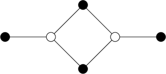
(a) The graph $S_{-}^{2}(s^{3})$

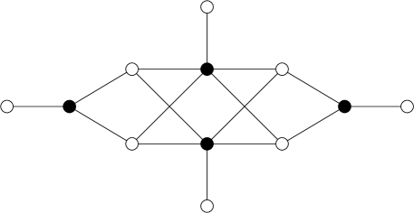
(b) The graph $S_{-}^{2}(S_{-}^{2}(s^{3}))$

Fig. 3: Examples of star expansion

Examples of graphs obtained by star expansion are shown in Fig. 3. From Theorem 3 we can obtain two different graphs, by choosing in which partition of $G$ we substitute vertices by $e^{m}$. In our examples, when the partitions of $G$ are of unequal size, we write $S_{+}^{m}(G)$ when we substitute the vertices in the largest partition, and $S_{-}^{m}(G)$ when we substitute the vertices in the smallest partition. In the cases where the partitions are of equal size, $S^{m}(G)$ will give the same graph for both partitions in all examples in this paper. If $G$ is an $(r,k-r)$-bipartite graph, then $S^{m}(G)$ will be $(r+k(m-1),k-r)$-bipartite. Since its output is always bipartite, the star expansion construction can be iterated to obtain new ELC-preserved graphs, such as the graph $S_{-}^{2}(S_{-}^{2}(s^{3}))$ of order 12, shown in Fig. 3b. However, some of these iterated constructions can be simplified. For instance, it is easy to verify that $S_{+}^{m}(s^{k})=s^{km}$ and $S_{+}^{m_{2}}(S_{-}^{m_{1}}(s^{k}))=S_{-}^{m_{1}m_{2}}(s^{k})$.

For all $n\geq 3$, there is a non-bipartite ELC-preserved graph on $n$ vertices, namely the complete graph, denoted $c^{n}$. This graph has $n$ vertices, $v_{1},v_{2},\ldots,v_{n}$, of degree $n-1$. Clearly the graph is ELC-preserved, since for all edges $\{v_{i},v_{j}\}$, $N_{v_{i}}=N_{v_{j}}$, and hence the sets $A$ and $B$ in Fig. 2 are empty. The following more general construction gives us more non-bipartite ELC-preserved graphs.

Theorem 4 (Clique expansion).

Given an ELC-preserved graph $G$ on $k$ vertices and an integer $m>1$, we obtain an ELC-preserved non-bipartite graph $C^{m}(G)$ on $n=km$ vertices by substituting all vertices of $G$ with $c^{m}$.

Proof.

Let $\{u,v\}\in E$. Let $u$ be substituted by $u_{1},\ldots,u_{m}$, and let $v$ be substituted by $v_{1},\ldots,v_{m}$. ELC on any edge within a substituted subgraph, such as $\{u_{i},u_{j}\}$, must preserve $C^{m}(G)$, since $N_{u_{i}}=N_{u_{j}}$. Due to symmetries, it only remains to show that ELC on an edge $\{u_{i},v_{j}\}$ preserves $C^{m}(G)$. In the graph $G$, let $A=N_{u}^{v}$, $B=N_{v}^{u}$, and $C=N_{u}\cap N_{v}$. In the graph $C^{m}(G)$, $N_{u_{i}}^{v_{j}}=A_{1}\cup\cdots\cup A_{m}$, $N_{v_{j}}^{u_{i}}=B_{1}\cup\cdots\cup B_{m}$, and $N_{u_{i}}\cap N_{v_{j}}=(C_{1}\cup\cdots\cup C_{m})\cup U\cup V$, where $U=\{u_{1},\ldots,u_{m}\}\setminus\{u_{i}\}$ and $V=\{v_{1},\ldots,v_{m}\}\setminus\{v_{j}\}$. Let $X,Y\in\{A,B,C\}$, $X\neq Y$. All subgraphs in $C^{m}(G)$ induced on $X_{r}$ are isomorphic to subgraphs in $G$ induced on $X$. A vertex $x_{r}\in X_{r}$ is connected to a vertex $y_{s}\in Y_{s}$ in $C^{m}(G)$, for $1\leq r,s\leq m$ if and only if $x\in X$ is connected to $y\in Y$ in $G$. Hence, toggling pairs between $X_{r}$ and $Y_{s}$, for $1\leq r,s\leq m$, preserves $C^{m}(G)$ since toggling pairs between $X$ and $Y$ preserves $G$. (The fact that edges have been added between $X_{r}$ and $X_{t}$, for $1\leq r,t\leq m$, by the clique substitution, has no effect on this, since the subgraphs in $C^{m}(G)$ induced on $X_{r}\cup X_{t}$ are isomorphic for all $1\leq r,t\leq m$.) The final effect of ELC on $\{u_{i},v_{j}\}$ is to toggle all pairs between $U\cup V$ and $A_{1}\cup\cdots\cup A_{m}$, and all pairs between $U\cup V$ and $B_{1}\cup\cdots\cup B_{m}$. But, since we also swap $u_{i}$ and $v_{j}$, the total effect is equivalent to swapping $u_{r}$ and $v_{r}$ for all $1\leq r\leq m$. It follows that $C^{m}(G)^{(u_{i},v_{j})}$ is isomorphic to $C^{m}(G)$, and hence that $C^{m}(G)$ is ELC-preserved. ∎

(a) The graph $C^{2}(s^{3})$

(b) The graph $C^{2}(S_{-}^{2}(s^{3}))$

Fig. 4: Examples of clique expansion

Examples of graphs obtained by clique expansion are shown in Fig. 4. The output of a clique expansion will always be a non-bipartite graph, except for the trivial case $C^{2}(e^{1})=s^{2}$. However, the input can be a bipartite graph, and hence the construction can be combined with star expansion to obtain new ELC-preserved graphs, such as the graph $C^{2}(S_{-}^{2}(s^{3}))$ of order 12, shown in Fig. 4b. Iterating clique expansion on its own does not produce new graphs, since, trivially, $C^{m}(c^{k})=c^{mk}$ and $C^{m_{2}}(C^{m_{1}}(G))=C^{m_{1}m_{2}}(G)$.

Definition 10.

Let the graph $h^{r}$ be an $(r,2^{r}-r-1)$-bipartite graph on $n=2^{r}-1$ vertices. To obtain $h^{r}$, let one partition, $U$, consist of $r$ vertices, and the other partition, $W$, be divided into $r-1$ disjoint subsets, $W_{i}$, for $2\leq i\leq r$, where $W_{i}$ contains $\binom{r}{i}$ vertices. Let each vertex in $W_{i}$ be connected to $i$ vertices in $U$, such that $N_{a}\neq N_{b}$ for all $a,b\in W$.

Theorem 5.

The graph $h^{r}$, for $r\geq 3$, is ELC-preserved and corresponds to the $[2^{r}-1,2^{r}-r-1,3]$ Hamming code.

Proof.

From the construction of the graph $h^{r}$, we see that it corresponds to a code with parity check matrix $(I\mid P)$, where the columns are all non-zero vectors from $\mathbb{F}_{2}^{r}$, which is the parity check matrix of a Hamming code [28]. We know from Theorem 1 that any ELC operation on $h^{r}$ must give a graph that corresponds to an equivalent code. Since the distance of the code is greater than two, all columns of the parity check matrix must be distinct. It follows that all parity check matrices of equivalent codes must contain all non-zero vectors from $\mathbb{F}_{2}^{r}$, in some order. Hence the corresponding graphs are isomorphic, and $h^{r}$ must be ELC-preserved. ∎

A graph is even if all its vertices have even degree, and odd if all its vertices have odd degree. (Connected even graphs are also known as Eulerian graphs.) An odd graph must have even order, and is always the complement of an even graph. Odd graphs have been shown to correspond to Type II self-dual additive codes over $\mathbb{F}_{4}$ [12].

Lemma 1.

Let $G=(V,E)$ be an odd graph. After performing any LC or ELC operation on $G$, we obtain a graph $G^{\prime}$ which is also odd.

Proof.

Let $v\in V$ and $w\in N_{v}$. LC on $v$ transforms $N_{w}$ into $N_{w}^{\prime}=(N_{w}\cup N_{v})\setminus(N_{w}\cap N_{v})\setminus\{w\}$, where $\left|N_{w}^{\prime}\right|=\left|N_{w}\right|+\left|N_{v}\right|-(2\left|N_{w}\cap N_{v}\right|+1)$. Since $G$ is odd, $\left|N_{w}\right|$ and $\left|N_{v}\right|$ must be odd. We then see that $\left|N_{w}^{\prime}\right|$ is the sum of three odd numbers, and must therefore be odd. The same argument holds for all neighbors of $v$, so $G*v$ is odd. That ELC also preserves oddness then follows from Definition 2. ∎

Definition 11.

Let the graph $h^{r}_{e}$ be an $(r+1,2^{r}-r-1)$-bipartite graph on $n=2^{r}$ vertices. To obtain $h^{r}_{e}$, first construct $h^{r}$, as in Definition 10, and then add a new vertex which is connected by edges to all existing vertices of even degree.

Theorem 6.

The graph $h^{r}_{e}$, for $r\geq 3$, is ELC-preserved and corresponds to the $[2^{r},2^{r}-r-1,4]$ extended Hamming code.

Proof.

$h^{r}_{e}$ must be bipartite, since all vertices of $h^{r}$ in the partition of size $r$ have degree $\sum_{i=2}^{r}\binom{r}{i}\frac{i}{r}=2^{r-1}-1$, which is odd. The new vertex added to $h^{r}$ also has odd degree, since the number of vertices in $h^{r}$ of even degree is $\sum_{i=1}^{\lfloor\frac{r}{2}\rfloor}\binom{r}{2i}=2^{r-1}-1$. Hence $h^{r}_{e}$ is odd. It follows from the construction that $h^{r}_{e}$ corresponds to a code with parity check matrix $(I\mid P)$, where the columns are all odd weight vectors from $\mathbb{F}_{2}^{r+1}$, which is the parity check matrix of an extended Hamming code [28]. We know from Theorem 1 that any ELC operation on $h^{r}_{e}$ must give a graph that corresponds to an equivalent code. Since the distance of the code is greater than two, all columns of the parity check matrix must be distinct. The graph $h^{r}_{e}$ is odd, and must remain so after ELC, according to Lemma 1. It follows that all parity check matrices of equivalent codes must contain all odd weight vectors from $\mathbb{F}_{2}^{r+1}$, in some order. Hence the corresponding graphs are isomorphic, and $h^{r}_{e}$ must be ELC-preserved. ∎

For $n=7$, we obtain from Theorem 5 the bipartite ELC-preserved graph $h^{3}$, shown in Fig. 5a, corresponding to the Hamming code of length 7. This is an important graph, as it forms the basis for the general constructions given by Theorems 7 and 8. The graph $h^{3}_{e}$ is shown in Fig. 5b.

(a) The graph $h^{3}$

(b) The graph $h^{3}_{e}$

Fig. 5: ELC preserved graphs from Hamming codes

Definition 12.

Given a graph $G=(V,E)$ on $k$ vertices, let the Hamming expansion $H(G)$ be a graph on $n=7k$ vertices constructed as follows. For all vertices $v_{i}\in V$, $0\leq i<k$, we replace $v_{i}$ by the subgraph $h_{i}$ with vertices $\{w_{7i},\ldots,w_{7i+6}\}$ and edges $\{\{w_{7i},w_{7i+3}\}$, $\{w_{7i},w_{7i+4}\}$, $\{w_{7i+1},w_{7i+3}\}$, $\{w_{7i+1},w_{7i+5}\}$, $\{w_{7i+2},w_{7i+4}\}$, $\{w_{7i+2},w_{7i+5}\}$, $\{w_{7i+3},w_{7i+6}\}$, $\{w_{7i+4},w_{7i+6}\}$, $\{w_{7i+5},w_{7i+6}\}\}$. (Note that $h_{i}$ is a specific labeling of the graph $h^{3}$. The labeled graph $h_{0}$ is depicted in Fig. 5a.) If $\{v_{i},v_{j}\}\in E$, we connect each of the vertices $w_{7i}$, $w_{7i+1}$, and $w_{7i+2}$ to all the vertices $w_{7j}$, $w_{7j+1}$, and $w_{7j+2}$. (Note that this differs from the graph substitution in Definition 8.) As an example, consider the graph $H(s^{2})$ shown in Fig. 6.

Theorem 7 (Hamming expansion).

The graph $H(G)$ is ELC-preserved if $G$ is ELC-preserved.

Proof.

Let $a=w_{6}$, $b=w_{3}$, and $c=w_{0}$. If $k>1$, let $d=w_{7}$, and assume (without loss of generality) that there is an edge $\{v_{0},v_{1}\}\in E$. Due to the symmetry of $H(G)$ and ELC-preservation of $G$, we only need to consider ELC on the three edges $\{a,b\}$, $\{b,c\}$, and $\{c,d\}$ to prove the ELC-preservation of $H(G)$. That $h_{0}$ is ELC-preserved, and hence that $\{a,b\}$ preserves $H(G)$ is easily verified by hand. We then consider the edge $\{b,c\}$. Note that $N_{b}^{c}=\{a,c^{\prime}=w_{1}\}$, where $c^{\prime}$ has exactly the same neighbors as $c$ outside $h_{0}$, and $a$ has no common neighbors with $c$ outside $h_{0}$. Since we know that the subgraph $h_{0}$ is ELC-preserved, the effect of ELC on $\{b,c\}$ is simply to swap $a$ and $c^{\prime}$. The edge $\{c,d\}$ corresponds to the edge $\{v_{0},v_{1}\}\in E$. In the graph $G$, let $A=N_{v_{0}}^{v_{1}}$, $B=N_{v_{1}}^{v_{0}}$, and $C=N_{v_{0}}\cap N_{v_{1}}$. In the graph $H(G)$, $c$ is connected to three copies of $A$, $d$ is connected to three copies of $B$, and both $c$ and $d$ are connected to three copies of $C$. Since ELC on $\{v_{0},v_{1}\}$ preserves $G$, toggling pairs between these multiplied neighborhoods must preserve $H(G)$, as in Theorem 4. There are only eight remaining vertices to consider: $c$ is connected to $D=\{w_{3},w_{4}\}$ and $E=\{w_{8},w_{9}\}$, and $d$ is connected to $F=\{w_{10},w_{11}\}$ and $G=\{w_{1},w_{2}\}$. The vertices in $D$ have no neighbors outside $h_{0}$, and the vertices in $F$ have no neighbors outside $h_{1}$. The vertices in $E$ share the same neighbors as $d$ outside $h_{1}$, and the vertices in $G$ share the same neighbors as $c$ outside $h_{0}$. The effect of ELC on $\{c,d\}$ is to swap $D$ with $E$ and $F$ with $G$. Hence $H(G)$ must be preserved, except for the local structure of $h_{0}$ and $h_{1}$, which it remains to check. ELC on $\{c,d\}$ has the effect of toggling pairs between $D$ and $G$ and between $E$ and $F$. Finally we swap $u$ and $v$. The result is that the structure of $h_{0}$ and $h_{1}$ is preserved, as illustrated in Fig. 6 and Fig. 7. It follows that $H(G)$ is ELC-preserved. ∎

Fig. 6: The graph $H(s^{2})$

Fig. 7: The graph $H(s^{2})^{(w_{0},w_{7})}$

Theorem 8 (Hamming clique expansion).

For $k\geq 1$ and $m\geq 1$, we obtain an ELC-preserved graph $H_{k}^{m}$ on $n=7k+m$ vertices by taking the union of $G=H(c^{k})$ and $K=c^{m}$. We add edges from each vertex in $K$ to all the $3k$ vertices in $G$ labeled (as in Theorem 7) $w_{7i}$, $w_{7i+1}$, and $w_{7i+2}$, for $0\leq i<k$. (Note that $H_{1}^{1}=h^{3}_{e}$.) As an example, the graph $H_{3}^{3}$ is shown in Fig. 8.

Proof.

Without loss of generality, let $a=w_{6}$, $b=w_{3}$, $c=w_{0}$, $d=w_{7}$, and let $e$ and $f$ be two distinct vertices in $K$. (For $k=1$, ignore $d$, and for $m=1$, ignore $f$.) Due to the symmetry of $H_{k}^{m}$, we only need to consider ELC on the five edges $\{a,b\}$, $\{b,c\}$, $\{c,d\}$, $\{c,e\}$, and $\{e,f\}$ to prove the ELC-preservation of $H_{k}^{m}$. The proof for $\{a,b\}$, $\{b,c\}$, and $\{c,d\}$ are the same as in Theorem 7. (The proof still works with $K=c^{m}$ added to $N_{c}$ and $N_{d}$.) The edge $\{e,f\}$ is trivial, since $N_{e}=N_{f}$. It only remains to show that ELC on $\{c,e\}$ preserves $H_{k}^{m}$. Observe that $N_{c}^{e}=\{w_{3},w_{4}\}$ and $N_{e}^{c}=\{w_{1},w_{2}\}$. All other neighbors of $c$ and $e$ are in $N_{c}\cap N_{e}$, since the underlying graph of $G=H(c^{k})$ is a complete graph. Furthermore, $w_{1}$ and $w_{2}$ are connected to all vertices in $N_{c}\cap N_{e}$, and $w_{3}$ and $w_{4}$ are not connected to any vertex in $N_{c}\cap N_{e}$. The effect of ELC is to swap the vertices in $N_{c}^{e}$ with the vertices in $N_{e}^{c}$. $h_{0}$ is preserved as before. It follows that $H_{k}^{m}$ is ELC-preserved. ∎

Fig. 8: The graph $H_{3}^{3}$

Proposition 1.

$H(G)$ is bipartite when $G=(V,E)$ is bipartite. $H_{k}^{m}$ is bipartite only in the trivial case where $k=m=1$.

Proof.

Let $V=\{v_{0},\ldots v_{k-1}\}$. In $H(G)$, each $v_{i}$ is replaced by a bipartite subgraph, $h_{i}$, and edges are added between these subgraphs, such that the induced subgraph on $\{w_{7i},$ $w_{7i+1},$ $w_{7i+2},$ $w_{7j},$ $w_{7j+1},$ $w_{7j+2}\}$ in $H(G)$ is a complete bipartite graph if there is an edge $\{v_{i},v_{j}\}\in E$ and an empty graph otherwise. It follows that $H(G)$ is bipartite whenever $G$ is bipartite. (The trivial case $H(e^{1})=h^{3}$ is clearly also bipartite.) $H_{k}^{m}$ is clearly non-bipartite if $k>2$ or $m>2$, since it contains a 3-clique. It is easily checked that for the remaining cases, only $H_{1}^{1}=h^{3}_{e}$ is bipartite. ∎

5 Classification

Tables 2 and 3 show how all bipartite ELC-preserved graphs of order $n\leq 16$, and all non-bipartite ELC-preserved graphs of order $n\leq 12$ arise from the constructions described in the previous section.

Table 2: Classification of bipartite ELC-preserved graphs

$n$
2	$s^{2}$
3	$s^{3}$
4	$s^{4}$
5	$s^{5}$
6	$s^{6}$, $S_{-}^{2}(s^{3})$
7	$s^{7}$, $h^{3}$
8	$s^{8}$, $S_{-}^{2}(s^{4})$, $h^{3}_{e}$
9	$s^{9}$, $S_{-}^{3}(s^{3})$
10	$s^{10}$, $S_{-}^{2}(s^{5})$
11	$s^{11}$
12	$s^{12}$, $S_{-}^{2}(s^{6})$, $S_{-}^{3}(s^{4})$, $S_{-}^{4}(s^{3})$, $S_{-}^{2}(S_{-}^{2}(s^{3}))$
13	$s^{13}$
14	$s^{14}$, $S_{-}^{2}(s^{7})$, $S_{-}^{2}(h^{3})$, $S_{+}^{2}(h^{3})$, $H(s^{2})$
15	$s^{15}$, $S_{-}^{3}(s^{5})$, $S_{-}^{5}(s^{3})$, $h^{4}$
16	$s^{16}$, $S_{-}^{2}(s^{8})$, $S_{-}^{4}(s^{4})$, $S_{-}^{2}(S_{-}^{2}(s^{4}))$, $S^{2}(h^{3}_{e})$, $h^{4}_{e}$

Table 3: Classification of non-bipartite ELC-preserved graphs

$n$
3	$c^{3}$
4	$c^{4}$
5	$c^{5}$
6	$c^{6}$, $C^{2}(s^{3})$
7	$c^{7}$
8	$c^{8}$, $C^{2}(s^{4})$
9	$c^{9}$, $C^{3}(s^{3})$, $H_{1}^{2}$
10	$c^{10}$, $C^{2}(s^{5})$, $H_{1}^{3}$
11	$c^{11}$, $H_{1}^{4}$
12	$c^{12}$, $C^{2}(s^{6})$, $C^{3}(s^{4})$, $C^{4}(s^{3})$, $C^{2}(S_{-}^{2}(s^{3}))$, $H_{1}^{5}$

We observe that certain pairs of ELC-preserved graphs are LC-equivalent. It is easy to verify that $c^{n}$ and $s^{n}$ form a complete LC orbit, for all $n\geq 3$. The following theorem explains all the remaining pairs of LC-equivalent ELC-preserved graphs for $n\leq 12$, namely $\{S_{-}^{2}(s^{4}),C^{2}(s^{4})\}$, $\{S_{-}^{2}(s^{6}),C^{2}(s^{6})\}$, $\{S_{-}^{3}(s^{4}),C^{3}(s^{4})\}$, and $\{S_{-}^{2}(S_{-}^{2}(s^{3})),C^{2}(S_{-}^{2}(s^{3}))\}$. (Note that all these pairs of graphs are part of larger LC orbits whose other members are not ELC-preserved.)

Theorem 9.

Let $G=(U\cup W,E)$ be a $(r,n-r)$-bipartite graph with partitions $U=\{u_{1},\ldots,u_{r}\}$ and $W=\{w_{1},\ldots,w_{n-r}\}$. Let $S^{m}(G)$ be the graph where the vertices in $U$ are substituted with $e^{m}$. If all vertices in $U$ have odd degree, and all pairs of vertices from $U$ have an even number of (or zero) common neighbors, then $C^{m}(G)=S^{m}(G)*w_{1}*\cdots*w_{n-r}$, i.e., we can get from $S^{m}(G)$ to $C^{m}(G)$ by performing LC on all vertices in $W$. (The order of the LC operations is not important.)

Proof.

Consider performing LC on a vertex $w_{i}$ in $S^{m}(G)$. This vertex will be connected to the set $X$ of $m-1$ pendant vertices, and to $km$ other vertices, where $k$ is the degree of $w_{i}$ in $G$. Let $u$ be a neighbor of $w_{i}$ in $G$, and let $Y$ be the set of $m$ vertices that $u$ is replaced with in $S^{m}(G)$. The subgraph induced on $Y$ is $e^{m}$. After LC on $w_{i}$, the induced subgraph on $Y$ will be $c^{m}$. Moreover, the induced subgraph on $X\cup\{w_{i}\}$ will also be $c^{m}$, and all vertices in $Y$ will be connected to all vertices of $X\cup\{w_{i}\}$. Subsequent LC on another vertex $w_{j}$, where $w_{j}$ is also connected to $u$ in $G$, will change the subgraph induced on $Y$ back to $e^{m}$. To ensure that the induced subgraph on $Y$ is $c^{m}$ in the final graph, we must require $u$ to have odd degree in $G$. If $w_{i}$ is also connected to another vertex $u^{\prime}$ in $G$, which is replaced by $Y^{\prime}$ in $S^{m}(G)$, LC on $w_{i}$ will connect all vertices in $Y$ to all vertices in $Y^{\prime}$. Since we require that $u$ and $u^{\prime}$ share an even number of neighbors, none of these edges will remain in the final graph. With these considerations, it follows that after performing LC on all vertices in $W$, we obtain a graph where every vertex of $G$ is substituted by $c^{m}$, which is the definition of $C^{m}(G)$. ∎

New non-bipartite ELC-preserved graphs, $h^{r}_{*}$, of order $n=2^{r}$ for $r\geq 4$, can be obtained from the following theorem, by applying the given LC operations to ELC-preserved bipartite graphs corresponding to extended Hamming codes, $h^{r}_{e}$. The smallest example of this, $h^{4}_{*}$, is shown in Fig. 9b. (Note that $h^{3}_{*}=h^{3}_{e}$. For $r\geq 4$, $h^{r}_{*}$ is a non-bipartite ELC-preserved graph that cannot be obtained from any of our other constructions.)

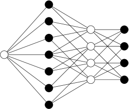
(a) The Graph $h^{4}_{e}$

(b) The Graph $h^{4}_{*}$

Fig. 9: Example of new ELC-preserved graph obtained by LC

Theorem 10.

Given the bipartite ELC-preserved graph $h^{r}_{e}$, defined in Definition 11, then $2^{r}-r-1$ LC operations applied, in any order, one to each vertex in the partition of size $2^{r}-r-1$, preserve the graph, while $r+1$ LC operations applied, in any order, one to each vertex in the partition of size $r+1$ gives an ELC-preserved graph $h^{r}_{*}$ which is non-bipartite when $r\geq 4$.

Proof.

Let $U$ denote the set of vertices in the partition of size $r+1$, and $W$ denote the set of vertices in the partition of size $2^{r}-r-1$. After performing LC on all vertices in $W$, two vertices $u,v\in U$ will be connected by an edge if and only if $u$ and $v$ have an odd number of common neighbors in $W$. To show that LC on all vertices in $W$ preserves $h^{r}_{e}$, we must show that all pairs of vertices from $U$ have an even number of common neighbors. Let $u_{e}$ be the extension vertex that was added to $h^{r}$ to form $h^{r}_{e}$, as described in Definition 11, and let $u_{i}$ and $u_{j}$ be two other vertices in $U$. The number of neighbors common between $u_{e}$ and $u_{i}$ is $\sum_{i=1}^{\lfloor\frac{r}{2}\rfloor}\binom{r}{2i}\frac{2i}{r}=2^{r-2}$. The number of neighbors common between $u_{i}$ and $u_{j}$ is $\sum_{i=2}^{r}\binom{r-2}{i-2}=2^{r-2}$.

We will now show that LC on all vertices in $U$ transforms $h^{r}_{e}$ into the ELC-preserved graph $h^{r}_{*}$. The adjacency matrix of $h^{r}_{e}$ can be written $\Gamma=\begin{pmatrix}\boldsymbol{0}_{r\times r}&P\\ P^{\text{T}}&\boldsymbol{0}_{(n-r)\times(n-r)}\end{pmatrix}$, where $(I\mid P)$ is the parity check matrix of $\mathcal{C}$, an extended Hamming code. LC on a vertex $u\in U$ can be implemented on $\Gamma$ by adding row $u$ to all rows in $N_{u}$ and then changing the diagonal elements $\Gamma_{v,v}$, for all $v\in N_{u}$, from 1 to 0. After performing LC on all vertices in $U$, the adjacency matrix of $h^{r}_{*}$ is $M=\begin{pmatrix}\boldsymbol{0}&P\\ P^{\text{T}}&X\end{pmatrix}$. Since each vertex in $W$ has an odd number of neighbors in $U$, each row of $X$ is the linear combination of an odd number of rows from $P$, except that all diagonal elements of $X$ have been changed from 1 to 0. Moreover, the non-zero coordinates of row $i$ of $P^{T}$ indicate which rows of $P$ were added to form row $i$ of $X$. It follows that the rows of the matrix $\begin{pmatrix}I&P\\ P^{\text{T}}&X+I\end{pmatrix}$ are the $2^{r}$ codewords of $\mathcal{C}^{\perp}$ formed by taking all linear combinations of an odd number of rows from $(I\mid P)$, since $(I\mid P)$ contains all odd weight columns from $\mathbb{F}_{2}^{r+1}$. After performing ELC on an edge $\{u,v\}$ in $h^{r}_{*}$, where $u\in U$ and $v\in W$, and then swapping vertices $u$ and $v$, we obtain an adjacency matrix $M^{\prime}=\begin{pmatrix}\boldsymbol{0}&P^{\prime}\\ {P^{\prime}}^{\text{T}}&X^{\prime}\end{pmatrix}$. After ELC on an edge $\{u,v\}$ where $u,v\in W$, the vertices in $U$ will no longer be an independent set, but by permuting vertices from $U$ with vertices from $N_{u}$ or $N_{v}$, we can obtain the form $M^{\prime}$. We need to show that the rows of $M^{\prime}+I$ are $2^{r}$ codewords of a code equivalent to $\mathcal{C}^{\perp}$ formed by taking linear combinations of an odd number of rows from $(I\mid P^{\prime})$. Since, according to Theorem 6, the extended Hamming code only has one parity check matrix, up to column permutations, this implies that $h^{r}_{*}$ is ELC-preserved. ELC on $\{u,v\}$ is the same as LC on $u$, followed by LC on $v$, followed by LC on $u$ again. We have seen that LC corresponds to row additions and flipping diagonal elements. We only need to show that all diagonal elements of $M$ are flipped from 1 to 0 an even number of times to ensure that all rows of $M^{\prime}+I$ are the codewords described above. If we swap vertices $u$ and $v$ after performing ELC, it follows from the definition of ELC that rows $u$ and $v$ of $M^{\prime}$ must be the same as in $M$. As for the other rows, LC on $u$ flips $M_{i,i}$ for $i\in N_{u}\setminus\{v\}$ , LC on $v$ then flips $M_{i,i}$ for $i\in(N_{v}\cup N_{u})\setminus(N_{v}\cap N_{u})$, and finally, LC on $u$ flips $M_{i,i}$ for $i\in N_{v}\setminus\{v\}$. In total, this means that for each $i\in N_{u}\cup N_{v}\setminus\{u,v\}$, the diagonal element $M_{i,i}$ has been flipped from 1 to 0 two times.

The graph $h^{r}_{*}$ is non-bipartite if there is at least one pair of vertices from $W$ with an odd number of common neighbors in $U$. For $r\geq 4$, there must be a pair of vertices from $W_{2}\subset W$, the set of $\binom{r}{2}$ vertices of degree $2$ in $h^{r}$, with no common neighbors in $h^{r}$ and hence one common neighbor, i.e. the extension vertex, in $h^{r}_{e}$. ∎

6 ELC-preserved Codes

As we have already shown, the graph $h^{3}$ corresponds to the $[7,4,3]$ Hamming code, and its dual $[7,3,4]$ simplex code. The graph $h^{3}_{e}$ corresponds to the self-dual $[8,4,4]$ extended Hamming code. The star graph $s^{n}$ corresponds to the $[n,1,n]$ repetition code, and its dual $[n,n-1,2]$ parity check code. We can obtain larger ELC-preserved bipartite graphs using Hamming expansion or star expansion, and the parameters of the corresponding codes are given by the following theorems.

Theorem 11.

For a connected ELC-preserved $(r,k-r)$-bipartite graph $G$ on $k\geq 2$ vertices, the graph $H(G)$ corresponds to a $[7k,3k+r,4]$ code $\mathcal{C}$, and to the dual $[7k,4k-r,4]$ code $\mathcal{C}^{\perp}$.

Proof.

From the construction of $H(G)$, we get that $\mathcal{C}$ must have length $n=7k$. The codes $\mathcal{C}$ and $\mathcal{C}^{\perp}$ have dimension $3k+r$ and $4k-r$, respectively, since $H(G)$ has partitions of size $3k+r$ and $4k-r$ when $G$ has partitions of size $r$ and $k-r$. That both $\mathcal{C}$ and $\mathcal{C}^{\perp}$ have minimum distance 4 follows from the fact that the minimum vertex degree in both partitions of $H(G)$ is 3. This is verified by observing that the subgraph $h_{0}$, shown in Fig. 5a, has one vertex $w_{6}$ of degree 3, and three vertices $w_{3}$, $w_{4}$, and $w_{5}$ of degree 3, belonging to different partitions. Moreover, the degrees of $w_{0}$, $w_{1}$, and $w_{2}$ must be at least 5, since $G$ is connected. ∎

Theorem 12.

Let $G$ be a connected ELC-preserved $(r,k-r)$-bipartite graph on $k\geq 2$ vertices and assume, without loss of generality, that $r\leq k-r$. Let $G$ correspond to a $[k,r,d]$ code and its dual $[k,k-r,d^{\prime}]$ code. Then $S_{+}^{m}(G)$ corresponds to an $[mk,r,md]$ code and its dual $[mk,mk-r,2]$ code. $S_{-}^{m}(G)$ corresponds to an $[mk,k-r,md^{\prime}]$ code and its dual $[mk,mk-k-r,2]$ code.

Proof.

From the construction of $S^{m}(G)$, we get that all the codes must have length $n=mk$. In $G$, the minimum vertex degree in the partition of size $r$ must be $d-1$, and the minimum vertex degree in the other partition must be $d^{\prime}-1$. In $S_{+}^{m}(G)$, $k-r$ vertices of $G$ have been substituted by $e^{m}$ and $m$ pendants have been added to the other $r$ vertices. Hence, $S_{+}^{m}(G)$ must contain a partition of size $r$ with minimum vertex degree $md-1$, since the vertex of degree $d-1$ in $G$ is now connected to $d-1$ copies of $e^{m}$ plus $m-1$ pendants. The other partition of $S_{+}^{m}(G)$ has size $mk-r$, and contains pendants, i.e., vertices of degree one. By similar argument, $S_{-}^{m}(G)$ has a partition of size $k-r$ with minimum vertex degree $md^{\prime}-1$ and a partition of size $mk-k-r$ with minimum vertex degree one. The dimensions and minimum distances of the corresponding codes follow. ∎

We observe that the ELC-preserved graphs $h^{3}_{e}$ and $H(s^{2})$ correspond to $[8,4,4]$ and $[14,7,4]$ self-dual codes. A natural question to ask is whether there are other ELC-preserved self-dual codes. All self-dual binary codes of length $n\leq 34$ have been classified by Bilous and van Rees [5, 4]. A database containing one representative from each equivalence class of codes with $n\leq 32$ and $d\geq 4$, and one representative from each equivalence class of codes with $n=34$ and $d\geq 6$ is available on-line at http://www.cs.umanitoba.ca/~umbilou1/. We have generated the ELC orbits of all the corresponding bipartite graphs, and found that $h^{3}_{e}$ and $H(s^{2})$ are the only ELC-preserved graphs, as shown in Table 4. However, as the following theorem shows, we can construct ELC-preserved self-dual codes with $n\geq 56$ by iterated Hamming expansion of $h^{3}_{e}$ and $H(s^{2})$.

Table 4: ELC orbit size of graphs corresponding to self-dual codes

$n$	$d$	Codes	ELC-preserved	Size two ELC orbits
8	$\geq 4$	1	1	-
10	$\geq 4$	-	-	-
12	$\geq 4$	1	-	1
14	$\geq 4$	1	1	-
16	$\geq 4$	2	-	1
18	$\geq 4$	2	-	-
20	$\geq 4$	6	-	1
22	$\geq 4$	8	-	-
24	$\geq 4$	26	-	2
26	$\geq 4$	45	-	-
28	$\geq 4$	148	-	1
30	$\geq 4$	457	-	-
32	$\geq 4$	2523	-	2
34	$\geq 6$	938	-	-

Theorem 13.

Let $H^{r}(G)=H(\cdots H(G))$ denote the $r$-fold Hamming expansion of $G$. Then for $r\geq 1$, $H^{r}(h^{3}_{e})$ corresponds to an ELC-preserved self-dual $[8\cdot 7^{r},4\cdot 7^{r},4]$ code, and $H^{r+1}(s^{2})$ corresponds to an ELC-preserved self-dual $[2\cdot 7^{r+1},7^{r+1},4]$ code.

Proof.

The parameters of the codes follows from Theorem 11. It remains to show that they are self-dual. A code with generator matrix $(I\mid P)$ is self-dual if the same code is also generated by $(P^{\text{T}}\mid I)$, i.e., if $P^{-1}=P^{\text{T}}$. The codes associated with both $h^{3}_{e}$ and $H(s^{2})$ have the property that $P=P^{\text{T}}$, and Hamming expansion must preserve this symmetry since it has the same effect on both partitions of the graph. In general, $P=P^{\text{T}}$ only implies that a code is isodual, but we can prove a stronger property in this case. Note that $P$ corresponding to $H(G)$ will have full rank when $P$ corresponding to $G$ has full rank, since we know that $P$ corresponding to $H(s^{2})$, which is the Hamming expansion of the induced subgraph on any pair of vertices connected by an edge in $G$, has full rank. Since an ELC-preserved code only has one generator matrix, up to column permutations, and the inverse of a symmetric matrix is symmetric, we must have that $P^{-1}(I\mid P)=(P\mid I)$. Hence the code is self-dual. ∎

7 Orbits of Size Two

ELC-preserved codes with good properties could have practical applications in iterative decoding [25, 22, 24, 23]. However, there seem to be extremely few such codes, and, except for the perfect Hamming codes, graphs arising from the constructions in Section 4 correspond to $[n,k,d]$ codes with either low minimum distance $d$ or low rate $\frac{k}{n}$, compared to the best known codes of the same length. Iterative decoding with ELC also works for graphs with larger ELC orbits, such as quadratic residue (QR) codes [22], and has performance close to that of iterative permutation decoding [19] for graphs with small ELC orbits, such as the extended Golay code [22]. The self-dual $[24,12,8]$ extended Golay code corresponds to a bipartite graph with an ELC orbit of size two. We have also found a $[15,5,7]$ Bose-Chaudhuri-Hocquenghem (BCH) code with an ELC-orbit of size two [24], but observed that larger QR and BCH codes have much larger orbits. As a generalization of ELC-preserved graphs, we now briefly consider graphs with ELC orbits of size two. The number of size two orbits are listed in Table 5.

We have also counted LC orbits of size two. (Note that the only connected graphs of order up to 12 which have LC orbits of size one are the trivial graphs of order one and two, and it remains an open problem to prove that these two graphs are the only graphs with LC orbits of size one.) Clearly there is an LC orbit $\{s^{n},c^{n}\}$ for all $n\geq 3$. The only other size two LC orbit we find for $n\leq 12$ is comprised of the two graphs of order six depicted in Fig. 10 (These two graphs correspond to the self-dual Hexacode over $\mathbb{F}_{4}$ [12].)

Table 5: Number of orbits of size two

$n$	Bipartite ELC	Non-bipartite ELC	LC
3	-	-	1
4	1	1	1
5	2	3	1
6	4	9	2
7	6	10	1
8	9	21	1
9	12	22	1
10	22	43	1
11	22	41	1
12	33	91	1
13	35
14	53
15	48

Fig. 10: LC orbit of size two

We have also looked at the ELC orbits corresponding to self-dual codes of length $n\leq 34$, as seen in Table 4. Except for the $[24,12,8]$ extended Golay code and a $[32,16,4]$ code, the remaining self-dual codes in this table with ELC orbits of size two, all with minimum distance four, can be constructed by the following theorem. It remains an open problem to devise a general construction for self-dual codes with ELC orbits of size two and minimum distance greater than four.

Theorem 14.

Let $G$ be a $(2m,2m)$-bipartite graph on $4m$ vertices, where $m\geq 3$. Let the vertices in one partition be labeled $v_{1},v_{2},\ldots,v_{2m}$, and the vertices in the other partition be labeled $w_{1},w_{2},\ldots,w_{2m}$. Let there be an edge $\{v_{i},w_{j}\}$ whenever $i\neq j$. Then $G$ has an ELC orbit of size two and corresponds to a self-dual $[4m,2m,4]$ code $\mathcal{C}$.

Proof.

The code $\mathcal{C}$ has generator matrix $(I\mid P)$ where $P$ is circulant with first row $(01\cdots 1)$. It can be verified that $P^{-1}=P=P^{\text{T}}$ when $P$ is of this form with even dimensions. Hence $P^{-1}(I\mid P)=(P^{\text{T}}\mid I)$ and $\mathcal{C}$ is self-dual. (An $(m,m)$-bipartite graph constructed as above for odd $m\geq 7$ would still have an ELC orbit of size two but would correspond to a non-self-dual $[2m,m,4]$ code.) Note that $m=1$ and $m=2$ must be excluded, since they produce the ELC-preserved graphs $s^{2}$ and $h^{3}_{e}$, respectively.

Due to the symmetry of $G$ we only need to consider ELC on one edge $\{v_{i},w_{j}\}$. This will take us to a graph $G^{\prime}$ where the neighborhoods of $v_{i}$, $v_{j}$, $w_{i}$, $w_{j}$ are unchanged, but where $N_{v_{k}}=\{v_{i},v_{j},w_{k}\}$ and $N_{w_{k}}=\{w_{i},w_{j},v_{k}\}$, for all $k\neq i,j$. We need to consider ELC on three types of edges in $G^{\prime}$. ELC on $\{v_{i},w_{j}\}$ or $\{v_{j},w_{i}\}$ will take us back to $G$. ELC on an edge $\{v_{k},w_{k}\}$ will preserve $G^{\prime}$, since it simply removes edges $\{v_{i},w_{j}\}$ and $\{v_{j},w_{i}\}$ and adds edges $\{v_{i},w_{i}\}$ and $\{v_{j},w_{j}\}$, thus in effect swapping vertices $v_{i}$ and $v_{j}$. Finally, ELC on an edge $\{v_{i},w_{k}\}$ also preserves $G^{\prime}$, since it swaps the roles of vertices $v_{j}$ and $v_{k}$. (ELC on $\{v_{k},w_{i}\}$ similarly swaps $w_{j}$ and $w_{k}$.) This can be seen by noting that $w_{k}$ has neighbors $v_{j}$ and $v_{k}$, with $v_{k}$ being connected to $w_{j}$ in $N_{v_{i}}^{w_{k}}$ and $v_{j}$ being connected to all vertices in $N_{v_{i}}^{w_{k}}$ except $w_{j}$. Hence these relations are reversed after complementation. Furthermore, $N_{v_{k}}\setminus N_{v_{i}}^{w_{k}}=N_{v_{j}}\setminus N_{v_{i}}^{w_{k}}=\{w_{k},w_{i}\}$, so isomorphism is preserved. We have shown that the ELC orbit of $G$ has size two. Since the minimum vertex degree over the ELC orbit is 3, the minimum distance of $\mathcal{C}$ is 4. ∎

8 Conclusions

We have introduced ELC-preserved graphs as a new class of graphs, found all ELC-preserved graphs of order up to 12 and all ELC-preserved bipartite graphs of order up to 16, and shown how all these graphs arise from general constructions. It remains an open problem to prove that all ELC-preserved graphs arise from these constructions, or give an example to the contrary. We therefore pose the following question.

Problem 1.

Is a connected ELC-preserved graph of order $n$ always either $s^{n}$, where $n$ is prime, $H_{k}^{m}$, where $n=7k+m$, $h^{r}$, where $n=2^{r}-1$, $h^{r}_{e}$ or $h^{r}_{*}$, where $n=2^{r}$, or can it be obtained as $S_{+}^{m}(G)$, $S_{-}^{m}(G)$, or $C^{m}(G)$, where $G$ is an ELC-preserved graph of order $\frac{n}{m}$, or $H(G)$, where $G$ is an ELC-preserved graph of order $\frac{n}{7}$?

Note that not all star graphs and complete graphs are primitive ELC-preserved graphs, since most of them can be obtained as follows. From the graph $e^{1}$, we can obtain all $c^{n}=C^{n}(e^{1})$. From $s^{2}=C^{2}(e^{1})$, we obtain all $s^{n}=S^{\frac{n}{2}}(s^{2})$ where $n$ is even. More generally, for $n=pq$ a composite number, $s^{n}=S_{+}^{p}(s^{\frac{n}{q}})=S_{+}^{q}(s^{\frac{n}{p}})$, so only $s^{p}$ with $p$ an odd prime is a primitive ELC-preserved graph.

Problem 2.

Enumerate or classify ELC-preserved graphs of order $n>12$ and ELC-preserved bipartite graphs of order $n>16$.

Our classification used a previous complete classification of ELC orbits [13], and a graph extension technique to obtain all bipartite ELC-preserved graphs of order 16. Perhaps the complexity of classification could be reduced by further exploiting restrictions on the structure of ELC-preserved graphs.

ELC-preserved graphs are an interesting new class of graphs from a theoretical point of view. As discussed in Section 1, LC and ELC orbits of graphs show up in many different fields of research, and ELC-preserved graphs may also be of interest in these contexts. We have seen that one possible use for bipartite ELC-preserved graphs is in iterative decoding of error-correcting codes. Hamming codes are perfect, but for this application we would like codes with rate $\frac{k}{n}\approx\frac{1}{2}$. Such ELC-preserved codes obtained from our constructions do not have minimum distance that can compete with the best known codes of similar length, except for the optimal $[8,4,4]$ code ($h^{3}_{e}$), for which iterative decoding has been simulated with good results [25], and the optimal $[14,7,4]$ code ($H(s^{2})$). Longer codes obtained from Hamming expansion will always have minimum distance 4, as shown in Theorem 11. Codes that have a negligible number of low weight codewords can still have good decoding performance, but the number of weight 4 codewords in these codes grows linearly with the length, since the number of degree 3 vertices in the corresponding graphs does so, and hence the codes are not well suited for this application. It is therefore interesting to consider ELC orbits of size two, one of them corresponding the extended Golay code of length 24, for which iterative decoding with ELC has been simulated with good results [22]. For codes of higher length, however, this criteria is probably also too restrictive. Graphs with ELC orbits of bounded size could be more suitable for this application, and would be interesting to study from a graph theoretical point of view. For some graphs, ELC on certain edges will preserve the graph, while ELC on other edges may not. Iterative decoding where only ELC on the subset of edges that preserve the graph are allowed has been studied [25]. Graphs where ELC on certain edges preserve the number of edges in the graph, or keep the number of edges within a given bound, have also been considered in iterative decoding [24]. ELC-preserved graphs are clearly a subclass of the graphs where all ELC orbit members have the same number of edges. This class of graphs, and other possible generalizations of ELC-preserved graphs, would be interesting to study further.

Acknowledgements

This research was supported by the Research Council of Norway. The authors would like to thank the anonymous reviewers for providing useful suggestions and corrections that improved the quality of the manuscript.

References

- [1] Aigner, M. and van der Holst, H.: “Interlace polynomials”. Linear Algebra Appl., 377, pp. 11–30, 2004.
- [2] Arratia, R., Bollobás, B., Coppersmith, D., and Sorkin, G. B.: “Euler circuits and DNA sequencing by hybridization”. Discrete Appl. Math., 104, pp. 63–96, 2000.
- [3] Arratia, R., Bollobás, B., and Sorkin, G. B.: “The interlace polynomial of a graph”. J. Combin. Theory Ser. B, 92(2), pp. 199–233, 2004.
- [4] Bilous, R. T.: “Enumeration of the binary self-dual codes of length 34”. J. Combin. Math. Combin. Comput., 59, pp. 173–211, 2006.
- [5] Bilous, R. T. and van Rees, G. H. J.: “An enumeration of binary self-dual codes of length 32”. Des. Codes Cryptogr., 26, pp. 61–86, 2002.
- [6] Bollobás, B.: Modern graph theory, volume 184 of Graduate Texts in Mathematics. Springer, New York, 1998.
- [7] Bouchet, A.: “Graphic presentations of isotropic systems”. J. Combin. Theory Ser. B, 45(1), pp. 58–76, 1988.
- [8] Bouchet, A.: “Circle graph obstructions”. J. Combin. Theory Ser. B, 60(1), pp. 107–144, 1994.
- [9] Briegel, H. J., Browne, D. E., Dür, W., Raussendorf, R., and Van den Nest, M.: “Measurement-based quantum computation”. Nature Phys., 5(1), pp. 19–26, 2009.
- [10] Calderbank, A. R., Rains, E. M., Shor, P. M., and Sloane, N. J. A.: “Quantum error correction via codes over GF(4)”. IEEE Trans. Inform. Theory, 44(4), pp. 1369–1387, 1998.
- [11] Curtis, R. T.: “On graphs and codes”. Geom. Dedicata, 41(2), pp. 127–134, 1992.
- [12] Danielsen, L. E. and Parker, M. G.: “On the classification of all self-dual additive codes over GF(4) of length up to 12”. J. Combin. Theory Ser. A, 113(7), pp. 1351–1367, 2006.
- [13] Danielsen, L. E. and Parker, M. G.: “Edge local complementation and equivalence of binary linear codes”. Des. Codes Cryptogr., 49, pp. 161–170, 2008.
- [14] Danielsen, L. E. and Parker, M. G.: “Interlace polynomials: Enumeration, unimodality, and connections to codes”. Discrete Appl. Math., 158(6), pp. 636–648, 2010.
- [15] de Fraysseix, H.: “Local complementation and interlacement graphs”. Discrete Math., 33(1), pp. 29–35, 1981.
- [16] Ellis-Monaghan, J. A. and Sarmiento, I.: “Distance hereditary graphs and the interlace polynomial”. Combin. Probab. Comput., 16(6), pp. 947–973, 2007.
- [17] Fon-der Flaas, D. G.: “On local complementations of graphs”. In Combinatorics (Eger, 1987), volume 52 of Colloq. Math. Soc. János Bolyai, pp. 257–266, North-Holland, Amsterdam, 1988.
- [18] Geelen, J. and Oum, S.: “Circle graph obstructions under pivoting”. J. Graph Theory, 61(1), pp. 1–11, 2009.
- [19] Halford, T. R. and Chugg, K. M.: “Random redundant iterative soft-in soft-out decoding”. IEEE Trans. Commun., 56(4), pp. 513–517, 2008.
- [20] Hein, M., Eisert, J., and Briegel, H. J.: “Multi-party entanglement in graph states”. Phys. Rev. A, 69(6), p. 062 311, 2004.
- [21] Joo, J. and Feder, D. L.: “Edge local complementation for logical cluster states”. New J. Phys., 13, p. 063 025, 2011.
- [22] Knudsen, J. G., Riera, C., Danielsen, L. E., Parker, M. G., and Rosnes, E.: “Iterative decoding on multiple Tanner graphs using random edge local complementation”. In Proc. IEEE Int. Symp. Inform. Theory, pp. 899–903, 2009.
- [23] Knudsen, J. G., Riera, C., Danielsen, L. E., Parker, M. G., and Rosnes, E.: “Improved adaptive belief propagation decoding using edge-local complementation”. In Proc. IEEE Int. Symp. Inform. Theory, pp. 774–778, 2010.
- [24] Knudsen, J. G., Riera, C., Danielsen, L. E., Parker, M. G., and Rosnes, E.: “Random edge-local complementation with applications to iterative decoding of HDPC codes”. Reports in Informatics 395, University of Bergen, August 2010.
- [25] Knudsen, J. G., Riera, C., Parker, M. G., and Rosnes, E.: “Adaptive soft-decision iterative decoding using edge local complementation”. In Second International Castle Meeting on Coding Theory and Applications – ICMCTA 2008, volume 5228 of Lecture Notes in Comput. Sci., pp. 82–94, Springer, Berlin, 2008.
- [26] Kotzig, A.: “Eulerian lines in finite 4-valent graphs and their transformations”. In Theory of Graphs (Proc. Colloq., Tihany, 1966), pp. 219–230, Academic Press, New York, 1968.
- [27] Parker, M. G. and Rijmen, V.: “The quantum entanglement of binary and bipolar sequences”. In Sequences and Their Applications – SETA ’01, Discrete Math. Theor. Comput. Sci., pp. 296–309, Springer, London, 2002.
- [28] Pless, V. S. and Huffman, W. C. (editors): Handbook of Coding Theory. North-Holland, 1998, Amsterdam.
- [29] Riera, C. and Parker, M. G.: “On pivot orbits of Boolean functions”. In Proc. Fourth International Workshop on Optimal Codes and Related Topics, pp. 248–253, Bulgarian Acad. Sci. Inst. Math. Inform., Sofia, 2005.
- [30] Riera, C. and Parker, M. G.: “Generalised bent criteria for Boolean functions (I)”. IEEE Trans Inform. Theory, 52(9), pp. 4142–4159, 2006.
- [31] Van den Nest, M., Dehaene, J., and De Moor, B.: “Graphical description of the action of local Clifford transformations on graph states”. Phys. Rev. A, 69(2), p. 022 316, 2004.