Robust approach to gravity
Abstract
We consider metric theories of gravity without mapping them to their scalar-tensor counterpart, but using the Ricci scalar itself as an “extra” degree of freedom. This approach avoids then the introduction of a scalar-field potential that might be ill defined (not single valued). In order to explicitly show the usefulness of this method, we focus on static and spherically symmetric spacetimes and deal with the recent controversy about the existence of extended relativistic objects in certain class of models.
pacs:
04.50.Kd, 04.40.Dg, 95.36.+xI Introduction
Modified theories of gravity are metric theories which postulate an a priori arbitrary function of the Ricci scalar as the Lagrangian density. These theories have been proposed to explain the late time accelerated expansion of the Universe as well as a mechanism to produce inflation in the early Universe in terms of geometry instead of introducing any dark energy ideas or a scalar inflaton accexp . Thanks to the above properties, these theories have become one of the most popular alternative theories of gravity. In recent years, several specific models have been analyzed in different settings (see Ref. f(R) , for a review). Although the early models were ruled out for failing several tests (like the Solar System experiments) new proposals were put forward to overcome such drawbacks. Nevertheless, a considerable amount of analysis and observational confrontation is still required in order to compare the preliminary successes of such theories with the great achievements of general relativity (GR). In particular, the models that were claimed to pass several cosmological and local tests have been scrutinized in the strong gravity regime only recently. In fact, the first studies concerning their ability to describe relativistic extended objects, like neutron stars, seem to give contradictory results. Using a model proposed by Starobinsky Starobinsky2007 , Kobayashi and Maeda Kobayashi2008 found that such relativistic objects were difficult to construct since a curvature singularity developed within the object. Later, this issue was reanalyzed by several authors Babichev2009 ; Upadhye2009 , who found that singularity-free relativistic objects can indeed be constructed, arguing that the conclusion reached in Kobayashi2008 was due to a bad choice of the matter model (i. e. the equation of state, hereafter EOS) Babichev2009 , while in Upadhye2009 it was claimed that a “chameleon” is the responsible for the existence of such “stars,” regardless of the EOS.
A common feature to all of the aforementioned works Kobayashi2008 ; Babichev2009 ; Upadhye2009 is that the analysis was performed by mapping the Starobinsky model to a scalar-tensor theory of gravity (STT) (cf. Faraoni2007 ). Under this mapping, the Ricci scalar has a behavior of the sort , where is the scalar-field associated with the corresponding STT and The key point is to determine if the dynamics of leads it or not to the value within the spacetime generated by the relativistic object. Irrespective of the different results and confusing explanations obtained in Kobayashi2008 ; Babichev2009 ; Upadhye2009 , we will argue that their conclusions are rather questionable due to the fact that the mapping to the STT is ill defined. To be more specific, the scalar-field potential used to study the dynamics of is not single valued and possesses pathological features. Since similar kind of singularities were also found in the cosmological setting Frolov2008 , it is then worrisome that the ill-defined potential play such a crucial role in those analyses (cf. Refs. Miranda2009 ; Goheer2009 for further criticisms. See also Nojiri2008 and references therein for a more detailed discussion on cosmological singularities in theories).
The goal of this communication is threefold: 1) to propose a straightforward and robust approach which consists in recasting the field equations in a more suitable way without mapping the original theory to any scalar-tensor counterpart. This method dispenses us from dealing with ill-defined quantities that might arise when performing such transformation; 2) to reanalyze carefully the issue about the existence of relativistic extended objects using our approach; 3) to stress that the analysis of theories based on the STT analogue with ill-defined quantities is not trustworthy, and that in cases where the STT approach is well defined (this depends on the specific model) it turns out to be rather convoluted and not very insightful. Since theories are still under close examination, a sound approach is required to treat them appropriately. This is the first step in that direction.
II theories of gravity
The general action for a theory of gravity is given by
| (1) |
where stands for the Ricci scalar, , and represents collectively the matter fields (we use units where ). The field equation arising from varying the action Eq. (1) with respect to the metric is
| (2) |
where and . It is straightforward to write the above equation in the following way
| (3) |
where . Taking the trace of this equation yields
| (4) |
where . Finally, using Eq. (4) in (II), we find
| (5) |
Equations (4) and (II) are the basic equations for gravity that we propose to treat in every application, instead of transforming them to STT. Now, several important remarks are in order regarding this set of equations. First, aside from the case , where the field equations reduce to those of GR, one is to consider functions such that (i. e. monotonically growing and convex functions) in order to avoid potential blowups in the field equations. These two conditions have been considered previously; the first one leads to a a positive definite gravitational “constant” when regarding theories as effective theories. The condition was suggested to avoid gravitational instabilities Dolgov2003 . Second, Eq. (II) supplies a second order equation for the metric provided that the Ricci scalar is considered as an independent field. This is possible thanks to Eq. (4) which provides the information needed to solve Eq. (II) for the metric alone (given a matter source).
As will become evident below, this approach is rather clean and free of the pathologies that can arise when mapping gravity to STT.
III Static and spherically symmetric spacetimes
In order to give some insight to the usefulness of our approach, we consider a static and spherically symmetric (SSS) spacetime with a metric given by , where the metric coefficients and are functions of the coordinate solely. The Ricci scalar as well as the matter variables will also be functions of . The analysis of this kind of spacetimes is interesting in many ways; however, we will focus here only on the issue about the existence (or absence thereof) of well behaved compact objects. Equation (4) yields
| (6) | |||||
(where ). From the , , and components of Eq. (II) and using also Eq. (6) we find
| (7) | |||||
| (8) | |||||
| (9) | |||||
Note that Eqs. (8) and (9) are not independent. In fact, one has the freedom of using one or the other (see Sec. IV below). Now, from the usual expression of in terms of the Christoffel symbols one obtains
| (10) | |||||
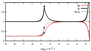
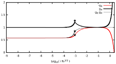
As one can check by a direct calculation, using Eqs. (7)(9) in Eq. (10) leads to an identity . This result confirms the consistency of our equations. When defining the first order variables and , Eqs. (6)(9) have the form , where , and therefore can be solved numerically. As far as we are aware, the system (6)(9) has not been considered previously (see Ref. Nzioki2010 for an alternative approach). These equations can be used to tackle several aspects of SSS spacetimes in gravity. Finally, we observe that for the above equations also reduce to the well known equations of GR for SSS spacetimes. When dealing with extended objects, notably those described by perfect fluids, the above equations are supplemented by the matter conservation equations. The Bianchi identities imply the conservation of the effective energy-momentum tensor [which corresponds to the right-hand-side (rhs) of Eq. (II)] which together with Eqs. (4) and (II) lead to the equation of conservation for the matter alone. So for a perfect fluid with , the conservation equation leads to [where is given explicitly by the rhs of Eq. (8)]. This is the modified Tolman-Oppenheimer-Volkoff equation of hydrostatic equilibrium to be complemented by an EOS.
In order to solve the differential equations some boundary conditions must be supplied, which in this case are rather regularity and asymptotic conditions. Regularity (smoothness) at implies the following expansion near : (where stands for or ). This implies at . We choose (local-flatness condition) and . The coefficients and associated with and the matter variables (and which correspond to the values of these quantities and its second derivatives evaluated at respectively) are related to each other. For instance, from the above power expansion and from Eqs. (9), (6) and (10), we find and , where the quantities at the rhs are evaluated at 111Note that in GR the field equations imply the algebraic relationship , which determine the value of in terms of the matter content solely. In theories this relationship is differential [cf. Eqs. (4) and (6)], and therefore the conditions for , and even for are not fixed in advance by the matter content only. We can recover the usual expressions of GR when taking ..
Now, as concerns the asymptotic conditions, we are interested in finding solutions that are asymptotically de Sitter, since the solutions are supposed to match a cosmological solution that represents the observed Universe. Therefore, we demand that asymptotically , where is a critical point (maximum or minimum) of a potential which is defined below. The value allows to define the effective cosmological constant as (like in GR with )222One can easily show that the system Eqs. (6)(9) in vacuum has the exact de Sitter solution , with and , which corresponds precisely where , as defined in the main text.. We mention that at the end of the numerical integration, we rescale in order to get the canonical asymptotic behavior . This rescaling amounts to redefine the coordinate. The asymptotic behavior depends on the value of . The details of the correlation between and depend on the matter model, and once this latter is fixed (for instance, an incompressible fluid with a given central pressure) the value can be found by a shooting method Numrec . Since we are interested in finding an exterior solution of Eq. (6) with (and ) asymptotically, we observe that such a solution exists if corresponds to a critical point of the “potential” . That is, is a point where vanishes [assuming in Eq. (6)] . This potential is radically different from the scalar-field potential that arises under the STT map. Furthermore, is as well defined as the function itself.
A technical difficulty that one faces when integrating the equations for neutron star models that asymptotically match realistic values of the cosmological constant is that a fortiori two completely different scales are involved. On one hand ; on the other (). That is, there are around 43 orders of magnitude between the typical density within a neutron star and the average density of the Universe. This ratio between densities naturally appears in the equations since the parameters which define the specific theory are of the order of , while the appropriate dimension within neutron stars is . So in units of , the cosmological constant turns out to be ridiculously small, while in units of , and turn out to be ridiculously large within the neutron star. So far, the authors that have studied relativistic objects in gravity Kobayashi2008 ; Babichev2009 ; Upadhye2009 ; Miranda2009 have faced this kind of technical problem, and, in order to avoid it, they have only constructed objects which are far from representing neutron stars embedded in a realistic de Sitter background. This means that either the background is realistic while the objects are ridiculously large (several orders of magnitude larger than a real neutron star) and not very dense, or the objects are realistic but is far too large. Such objects are relativistic in the sense that their pressure is of the same order of magnitude as their energy-density, and the ratio between a suitably defined mass and radius is not far from .
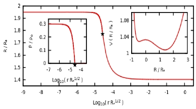
IV Numerical Results
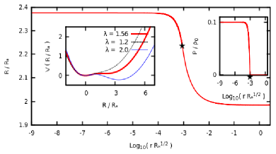
In order to test our method, we used first ( are positive constants; sets the scale), which was proposed in Ref. Miranda2009 . In that analysis the authors mapped the theory to the STT counterpart. However, unlike the Starobinsky model (see below), in this case the resulting scalar-field potential turns to be single valued and the authors of Miranda2009 did not find any singularity within the object. Under our approach, we associate to this the potential , where . This potential has several critical points. Figure 1 (top panel, right inset) depicts the potential for . Equations (6)(8) were integrated using a four-order Runge-Kutta algorithm by assuming an incompressible fluid with the same density and central pressure as in Miranda2009 . By implementing a shooting method Numrec , we found a solution for that goes from the global minimum of the potential to a positive value. The minimum at corresponds to the de Sitter value and gives rise to the effective cosmological constant . Figure 1 (top panel) depicts the solution for , the pressure (top panel, left inset) and the metric potentials (bottom panel) plotted up to the value where reaches the cosmological horizon given by . We checked that asymptotically the metric potentials matched perfectly well the de Sitter solution . We also verified that our solution corresponds to the one found in Miranda2009 and also confirmed that no singularity whatsoever was encountered. Furthermore, we checked that the numerical solutions found using the system Eqs. (6)(8) and the system Eqs. (6),(7) and (9) gave the same results within a relative error no larger than and that for both systems the identity Eq. (10) was satisfied within a relative error of . In this way, we ensured that no mistakes were introduced in the code during the typing of the equations. We emphasize that for this model the condition is satisfied by construction but the condition is not in general. However, for the solutions we found, this latter is always satisfied, particularly at . Having analyzed the solutions for this , we turned our attention to the Starobinsky model given by with . This is the model analyzed in Kobayashi2008 ; Babichev2009 ; Upadhye2009 using the transformation to STT. For such a model, the associated scalar-field potential is multiple-valued (cf. Fig. 1 in Frolov2008 and Fig. 2 in Kobayashi2008 ). Despite the potential being ill-defined, the authors in Kobayashi2008 argue that in the particular region where the scalar-field is evaluated, the potential is nevertheless well defined. It seems suspicious that in Babichev2009 ; Upadhye2009 the odd features of the potential are not mentioned at all. Even if one tried to ignore the region where the potential is pathological and consider only the single-valued region, there is no guarantee that the ill-defined region will not play any role in more general settings than the very specific case of static and spherically symmetric compact objects. Modifications of the Starobinsky model by adding a quadratic term do not cure this pathology, as one can see in Fig. 5 of Dev2008 . As we stressed before, the solutions found in Kobayashi2008 ; Babichev2009 ; Upadhye2009 gave rise to a controversy since in Kobayashi2008 the authors found a singularity in the Ricci scalar within the extended object, while in Babichev2009 ; Upadhye2009 the authors did not. Following our approach, we get . This potential has a rich structure depending on the value of (such structure arises also for the potential discussed above for different values of ). Figure 2 (top panel, left inset) depicts the potential for three values of . There is a value below which the potential has only one critical point (the global minimum) located at . In this regime (), we have found only oscillatory solutions around the global minimum. For , three critical points appear, with a minimum always located at (). In view of this structure, several kinds of solutions are possible for any given value of . We have found solutions where asymptotically approaches a minimum of at , the local maximum, and also solutions where oscillates asymptotically around . An asymptotic oscillatory behavior around seems a priori not adequate to produce the required de Sitter background; we plan to analyze those solutions in more detail elsewhere. Here, we are only interested in showing a solution for which goes to (a local minimum). Figure 2 shows the numerical solution which is asymptotically de Sitter. As one can appreciate, no singularity in the Ricci scalar was encountered in this solution and never crosses the two real-valued zeros of (which correspond to ) nor those of at which blowups in the equations can be produced. Even if for the static and spherically symmetric solutions, one can avoid the zeros of and , the Starobinsky model does not satisfy the conditions in general, and so, in other settings (e. g. cosmology) one has to keep this in mind when solving the equations.
V Conclusions
We have devised a straightforward and robust approach to treat metric gravity without resorting to the usual mapping to scalar-tensor theories. With this method, it is possible to analyze in a rather transparent and well defined way several aspects of these alternative theories. In particular, we focused on the existence of relativistic extended objects embedded in a de Sitter background and concluded that for some models such objects can be constructed without ambiguity and without resorting to any dubious explanations based on the use of ill-defined quantities. It seems that the analysis of the solutions presented here as well as other (i. e. solutions that admit different de Sitter backgrounds, even possibly Minkowski backgrounds) can only be carried out easily following our method since our potential depicts many features in a rather clear and clean fashion that allows us to identify the critical points which can reach asymptotically.
Building realistic neutron stars with a realistic de Sitter background in gravity still remains a technical challenge. In the near future, we plan to study in more detail this issue along with other aspects of gravity using our approach.
Acknowledgements.
Special thanks are due to S. Jorás and D. Sudarsky. This work was partially supported by CONACyT Grant No. SEP-2004-C01-47209-F and by DGAPA-UNAM Grants No. IN119309-3, No. IN115310, and No. IN-108309-3.References
- (1) A. A. Starobinsky, Phys. Lett. B 91, 99 (1980); A. A. Starobinsky, Sov. Astron. Lett. B9, 302 (1983); S. M. Carroll, V. Duvvuri, M. Trodden, and M. S. Turner Phys. Rev. D 70, 043528 (2004); S. Capozziello, S. Carloni, and A. Troisi, Recent Research Developments in Astronomy and Astrophysics-RSP/AA/21-2003 (2003), astro-ph/0303041; G. Cognola, E. Elizalde, S. Nojiri, S. D. Odintsov, L. Sebastiani, S. Zerbini Phys. Rev. D 77, 046009 (2008); S. Nojiri, and S. D. Odintsov, Phys. Rev. D 68, 123512 (2003); S. Nojiri, and S. D. Odintsov, AIP Conf. Proc. 1115:212-217, 2009
- (2) S. Nojiri and S. D. Odintsov, Int. J. Geom. Meth. Mod. Phys. 4, 115 (2007); T. P. Sotiriou and V. Faraoni, Rev. Mod. Phys. 82, 451 (2010); S. Capozziello, M. De Laurentis, and V. Faraoni, arXiv:0909.4672; A. De Felice, and S. Tsujikawa, Living Rev. Relativity 13, 3 (2010)
- (3) A. A. Starobinsky, JETP Lett. 86, 157 (2007)
- (4) T. Kobayashi, and K. I. Maeda, Phys. Rev. D 78, 064019 (2008); T. Kobayashi, and K. I. Maeda, Phys. Rev. D 79, 024009 (2009)
- (5) E. Babichev, and D. Langlois, Phys. Rev. D 80, 121501(R) (2009); E. Babichev, and D. Langlois Phys. Rev. D 81, 124051 (2010)
- (6) A. Upadhye, and W. Hu, Phys. Rev. D 80, 064002 (2009)
- (7) N. Lanahan-Tremblay, and V. Faraoni, Class. Quant. Grav. 24, 5667 (2007)
- (8) A. V. Frolov, Phys. Rev. Lett. 101, 061103 (2008)
- (9) V. Miranda, S. E. Jorás, I. Waga, M. Quartin, Phys. Rev. Lett. 102, 221101 (2009)
- (10) N. Goheer, J. Larena, and P. K. S. Dunsby, Phys. Rev. D 80, 061301(R) (2009)
- (11) S. Nojiri, and S. D. Odintsov, Phys. Rev. D 78, 046006 (2008)
- (12) A. D. Dolgov, and M. Kawasaki, Phys. Lett. B 573, 1 (2003)
- (13) A. M. Nzioki, S. Carloni, R. Goswami, P. K. S. Dunsby Phys. Rev. D 81, 084028 (2010)
- (14) W. H. Press, B. P. Flannery, S. A. Teukolsky, and W. T. Vettering, Numerical Recipes, Cambridge University Press, 1989
- (15) A. Dev, E. Jain, S. Jhingan, S. Nojiri, M. Sami, and I. Thongkool, Phys. Rev. D 78, 083515 (2008)