Polyharmonic Daubechies type wavelets in Image Processing and Astronomy, II

Abstract: We consider the application of the polyharmonic subdivision wavelets to Image Processing, in particular to Astronomical Images. The results show an essential advantage over some standard multivariate wavelets and a potential for better compression.

Key words: Wavelet Analysis, Daubechies wavelet, Image Processing, Astronomical Images.

1 Introduction

In [5] we have constructed the basic elements of the polyharmonic Wavelet Analysis. There we have provided all details of the construction of the filters for the whole infinite family of father and mother wavelets. Here we will finalize the multivariate construction and provide experimental evidence of the power of the new wavelets.

2 Polyharmonic Wavelet Analysis

The Polyharmonic Wavelet Analysis arises in the context of the polyharmonic subdivision. In general, it is obtained when the (one-dimensional) polynomials of degree $2N-1$ are replaced by polyharmonic functions of degree $N.$ The main element of the construction is the application of the Fourier transform in $n$ variables in $\mathbb{R}^{n+1}.$ For simplicity we assume that the Image which we consider is a function $u\left(t,y\right),$ for $t\in\mathbb{R}$ and $2\pi-$periodic in $y\in\mathbb{R}^{n}.$ We have

$$u\left(t.y\right) =\sum_{\eta\in\mathbb{Z}^{n}}\widehat{u}_{\eta}\left(t\right)e^{i\left\langle\eta,y\right\rangle}\qquad\text{where the Fourier coefficients are}$$ (1)

$$\widehat{u}_{\eta}\left(t\right) =\frac{1}{\left(2\pi\right)^{n}}\int_{0}^{2\pi}\cdot\cdot\cdot\int_{0}^{2\pi}u\left(t.y\right)e^{-i\left\langle\eta,y\right\rangle}dy.$$

For every fixed $\eta\in\mathbb{Z}^{n}$ and $\xi=\left|\eta\right|$ we make Wavelet Analysis which is based on the non-stationary father and mother wavelets $\left\{\varphi_{m}^{\xi}\left(t\right)\right\}_{m\geq 0}$ and $\left\{\psi_{m}^{\xi}\left(t\right)\right\}_{m\in\mathbb{Z}}$ of Theorem 4. Recall that they have refinement coefficients $M_{j}^{\left[m\right],\xi}$ and $\left(-1\right)^{j}M_{1-j}^{\left[m\right],\xi}$ respectively, where the polynomial $M^{\left[m\right],\xi}\left(z\right)$ was defined at the end of [5]. This gives the wavelet expansion

$$u\left(t.y\right)=\sum_{m,j\in\mathbb{Z}}\sum_{\eta\in\mathbb{Z}^{n}}\gamma_{\eta,m,j}\psi_{m}^{\left|\eta\right|}\left(t-j\right)e^{i\left\langle\eta,y\right\rangle}.$$ (2)

We summarize the results in the following theorem, for the proofs we refer to [3].

Theorem 1

For every $\xi\geq 0$ the functions $\psi_{m}^{\xi}\left(t\right)$ generate a non-stationary MRA of $L_{2}\left(\mathbb{R}\right)$ by means of the definitions

$$V_{m}^{\xi} :=clos_{L_{2}\left(\mathbb{R}\right)}\left\{\varphi_{m}^{\xi}\left(t-j\right):j\in\mathbb{Z}\right\}$$

$$L_{2}\left(\mathbb{R}\right) =clos_{L_{2}\left(\mathbb{R}\right)}\left(\bigcup_{m\in\mathbb{Z}}V_{m}^{\left|\xi\right|}\right).$$

Here $clos_{L_{2}\left(\mathbb{R}\right)}$ denotes the usual closure in a linear and topological sense with respect to the space $L_{2}\left(\mathbb{R}\right).$ Respectively, the Wavelet Analysis spaces $W_{m}^{\left|\xi\right|}$ defined by means of

$$W_{m}^{\xi}\bigoplus V_{m}^{\xi}=V_{m+1}^{\xi}$$

are generated as

$$W_{m}^{\xi}=clos_{L_{2}\left(\mathbb{R}\right)}\left\{\psi_{m}^{\xi}\left(t-j\right):j\in\mathbb{Z}\right\}.$$

As in the polyspline Wavelet Analysis studied in [4], the one-dimensional MRA $V_{j}^{\left|\eta\right|}$ which is generated for every $\eta\in\mathbb{Z}^{n}$ is related to a ”polyharmonic MRA” $PV_{j}$ as $PV_{j}=\bigoplus_{\eta\in\mathbb{Z}^{n}}V_{j}^{\left|\eta\right|}$ by means of the Fourier transform formula (1). Respectively, we have also the polyharmonic Wavelet Analysis defined by $PV_{j}\bigoplus PW_{j}=PV_{j+1}$ and reduced to infinitely many one-dimensional Wavelet Analyses for every $\eta\in\mathbb{Z}^{n}$ in the form $PW_{j}=\bigoplus_{\eta\in\mathbb{Z}^{n}}W_{j}^{\left|\eta\right|}$ by means of the Fourier transform formula (1).

Respectively, the space

$$L_{2,per}\left(\mathbb{R}^{n+1}\right)=\left\{f\left(t,y\right):t\in\mathbb{R},\ y\in\mathbb{R}^{n};f\text{ is }2\pi-\text{periodic in }y\right\}$$

is generated by an infinite amount of orthogonal (non-stationary) mother wavelets

$$\left\{\psi_{m}^{\left|\eta\right|}\left(t\right)e^{i\left\langle\eta,y\right\rangle}:\eta\in\mathbb{Z}^{n},\ m\in\mathbb{Z}\right\}.$$ (3)

Although these wavelets do not have a compact support in direction $y,$ it is important to note that they have ”elongated support” in the $y$ direction, which plays an essential role for the sparseness of the ”edge representation” in the images, a point of view nicely described in [2], see also [6].

3 The algorithm

From the above it follows that the algorithm for Decomposition and Reconstruction of the Polyharmonic Subdivision Wavelet Analysis (PhSdWav) consists of a Fourier transform in direction $y$ and consecutive application, for every $\eta\in\mathbb{Z}^{n},$ of one-dimensional Wavelet Analysis in direction $t.$ It consists of the following steps:

1. As usually we take as first approximation to the image the image itself where the expansion is in terms of the scaling functions $\left\{\varphi_{m}^{\left|\eta\right|}\left(t\right)\right\}_{m\geq 0}.$

2. Transforming to Wavelet Domain - this is the main difference with the usual approach. Roughly speaking, we obtain $\widehat{u}_{\eta}\left(t\right)$ in formula (1) and make its Wavelet Analysis for every $\eta\in\mathbb{Z}^{n}$ which gives us the coefficients $\gamma_{\eta,m,j}$ in the wavelet expansion (2). Let us note that these coefficients are in general complex numbers.

3. Filtering the small (insignificant) coefficients by using a threshold parameter.

4. Quantizing the remaining coefficients.

5. Encoding by arithmetic coder.

The algorithm was written in Matlab.

4 Experiments with images

We apply our Wavelet Analysis to different classes of images – synthetic and real. We compare the results of our method PhSdWav with parameter $N=9$ (see [5]) against the $2d$ wavelet transform with Daubechies wavelets $db9$ (which are tensor product wavelets and correspond to the one-dimensional Daubechies wavelets with parameter $N=9$). We use the standard function $dwt2$ in Matlab which contains a large class of $2d$ wavelets, and $db9$ is one of the most used representatives. In all Figures below we first display on top-left the original image, on top-right is the result of PhSdWav compressed representation obtained by wavelet thresholding, and on the bottom is the result of the $db9$ compressed representation obtained by wavelet thresholding. In order to make comparison between our method PhSdWav and $db9$ we perform thresholding which results in equal PSNR.

4.1 Elongated support tests on $64\times 64$ pixel edges

For the proper compression and representation of images it is of fundamental importance to understand how the method applies to ”edges”. For that reason we will first show the performance of our method to some synthetic edge images.

4.1.1 Vertical edge

In this test the image is a vertical edge which is a function $f_{vert}\left(t,y\right)$ defined in the rectangle $\left[0,1\right]\times\left[0,1\right]$ by

$$f_{vert}\left(t,y\right):=\left\{\begin{array}[c]{c}0\qquad\text{for }0\leq t\leq 1/2\\ 1\qquad\text{for }1/2<t\leq 1\end{array}\right..$$

We take a sampling of $f\left(t,y\right)$ by a $64\times 64$ pixel image. The performance of the polyharmonic Wavelets and the $db9$ wavelets is provided in Table 1 and Figure 1 below.

Table 1.

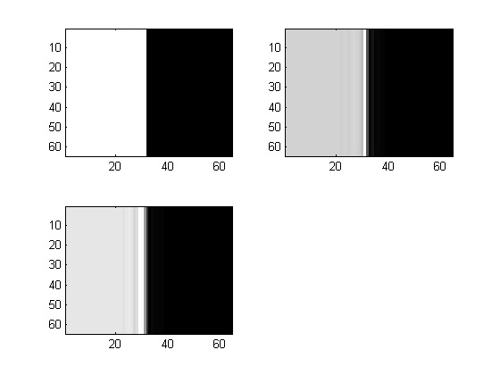
Figure 1: Vertical Edge

As we said above the wavelets of our basis (3) show elongation in direction $y$ and this makes the above image $f_{vert}$ perfect for representation and compression with the polyharmonic subdivision wavelets. We see that the quality of representation by means of PhSdWav (measured by the PSNR) is the same as the quality of representation by means of the standard $2-$dimensional Daubechies wavelet $db9$ but the number of coefficients is $20$ times less!

The image $f_{vert}$ would correspond to the one-dimensional image provided by the Heaviside function, $f\left(t\right)=0$ for $0\leq t\leq 1/2$ , $f\left(t\right)=1$ for $1/2<t\leq 1.$ The wavelets have an excellent performance for such images.

Just the opposite is the next example.

4.1.2 Horizontal edge

In this test the image is a horizontal edge, which is a function $f_{hor}\left(t,y\right)$ defined in the rectangle $\left[0,1\right]\times\left[0,1\right]$ by

$$f_{hor}\left(t,y\right):=\left\{\begin{array}[c]{c}0\qquad\text{for }0\leq y\leq 1/2\\ 1\qquad\text{for }1/2<y\leq 1\end{array}\right..$$

We take a sampling of $f_{hor}\left(t,y\right)$ by a $64\times 64$ pixel image. The performance of the polyharmonic Wavelets and the $db9$ wavelets is provided in Table 2 and Figure 2 below.

Table 2.

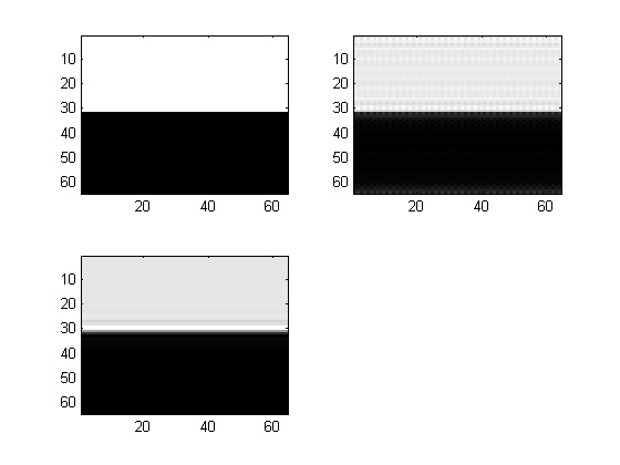
Figure 2: Horizontal Edge

We see now how inefficient the PhSdWav are for the representation of $f_{hor}$ compared to $db9$ wavelets, since for the same PSNR we need almost $3$ times more coefficients. This result is expected since PhSdWav has a very strong vertical orientation.

4.1.3 Skewed edge

Somewhere in the middle is the case of a skewed edge. In this test the image of skewed edge, which is a function $f_{skew}\left(t,y\right)$ defined in the rectangle $\left[0,1\right]\times\left[0,1\right]$ by (this is an approximate definition)

$$f_{skew}\left(t,y\right):=\left\{\begin{array}[c]{c}0\qquad\text{for }0\leq t\leq\frac{1}{6}\left(y+2.5\right)\\ 1\qquad\text{for }\frac{1}{6}\left(y+2.5\right)<t\leq 1\end{array}\right..$$

We take a sampling of $f_{skew}\left(t,y\right)$ by a $64\times 64$ pixel image. The performance of the polyharmonic Wavelets and the $db9$ wavelets is provided in Table 3 and Figure 3 below.

Table 3.

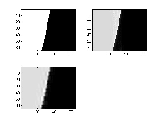
Figure 3: Skewed Edge

We see that although the edge is prettily skew (the slope is approximately $\tan\alpha=6$ ) the PhSdWav have a very nice performance compared to $db9.$

4.2 Lena image

Let us make a more detailed analysis of the seminal image of Lena in $128\times 128$ pixels. We provide the Compression Ratio and the Bits Encoded for both methods in Table 4 and Figure 4 below.

Table 4.

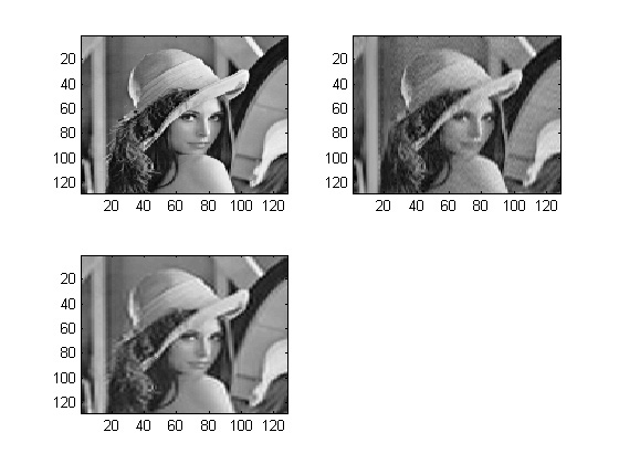
Figure 4: Lena Image

We see that for the same PSNR our method PhSdWav is better – it needs $20\%$ less coefficients. This is an astonishingly good result since as we have seen in the experiments with the synthetic edges in Section 4.1, our method of PhSdWav is adapted to the vertical direction $y$ and the Lena image does not have a dominating orientation of the edges.

4.3 Astronomical Images

Hereafter we analyze different types of astronomical images.

4.3.1 The Pleiades star cluster, a part with faint objects only, sized $128\times 128$

First we consider an image which is a part of the Pleiades image containing only faint stars. The results are provided in Table 5 and Figure 5 below.

Table 5.

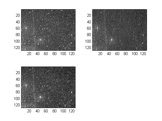
Figure 5: Pleiades star cluster, faint objects, 128x128 pixels

We see that for (almost) the same PSNR we have much less coefficients, the compression ratio is higher, and our entropy is much less, which shows a better potential for compression.

4.3.2 The Pleiades star cluster, a part with bright objects, sized $256\times 256$

Next we consider a part of the Pleiades containing several bright objects. The results are provided in Table 6 and Figure 6 below

Table 6.

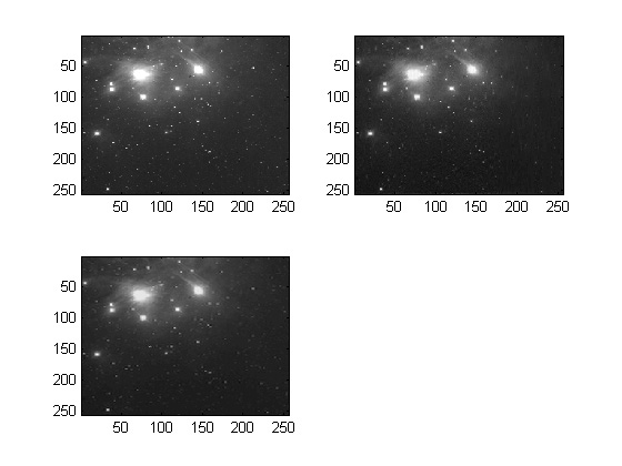
Figure 6: Pleiades star cluster, bright objects, 256x256 pixels

Again we see that for the same PSNR we have not only less coefficients but also a much higher compression ratio.

4.3.3 The Pleiades star cluster, chain, sized $128\times 128$

Here we consider a chain image of a part of the Pleiades image. The results are provided in Table 7 and Figure 7 below

Table 7.

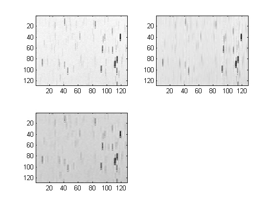
Figure 7: Pleiades star cluster, chain image, 128x128 pixels

For the same PSNR, the number of coefficients of our method PhSdWav is twice less than the number of $db9$ coefficients. This result is expected since the image is vertically oriented. However the compression ratio is not much bigger apparently due to more noise in the background of the image.

Acknowledgement. The first named author was sponsored partially by the Alexander von Humboldt Foundation, and all authors were sponsored by Project DO–2-275/2008 ”Astroinformatics” with Bulgarian NSF.

ABOUT THE AUTHORS

Ognyan Kounchev, Prof. Dr., Institute of Mathematics and Informatics, Bulgarian Academy of Science, tel. +359-2-9793851; kounchev@gmx.de

Damyan Kalaglarsky, Institute of Astronomy, Bulgarian Academy of Science, tel. +359-2-9793851; damyan@skyarchive.org.

Milcho Tsvetkov, Assoc. Prof., Dr., Institute of Astronomy, Bulgarian Academy of Science, tel. +359-2-9795935; milcho@skyarchive.org.

References

- [1] I. Daubechies, Ten lectures on wavelets, SIAM,
- [2] E. Candes, D. Donoho, Curvelets: A surprisingly effective nonadaptive representation of objects with edges, Curves and Surfaces, Larry L. Schumaker (eds.), by Vanderbilt University Press, Nashville, TN,
- [3] N. Dyn, O. Kounchev, D. Levin, H. Render, Polyharmonic subdivision for CAGD and multivariate Daubechies type wavelets, preprint,
- [4] O. Kounchev, Multivariate polysplines: Applications to Numerical and Wavelet Analysis, Academic Press, San Diego-London,
- [5] O. Kounchev, D. Kalaglarsky, Polyharmonic Daubechies type wavelets in Image Processing and Astronomy, I, present volume.
- [6] S. Mallat, G. Peyre, A Review of Bandlet Methods for Geometrical Image Representation, Numerical Algorithms, Vol. 44(3), p. 205-234, March 2007.