Analysis of Kepler’s short-cadence photometry for TrES-2b

Abstract

We present an analysis of 18 short-cadence (SC) transit lightcurves of TrES-2b using quarter 0 (Q0) and quarter 1 (Q1) from the Kepler Mission. The photometry is of unprecedented precision, 237 ppm per minute, allowing for the most accurate determination of the transit parameters yet obtained for this system. Global fits of the transit photometry, radial velocities and known transit times are used to obtain a self-consistent set of refined parameters for this system, including updated stellar and planetary parameters. Special attention is paid to fitting for limb darkening and eccentricity. We place an upper limit on the occultation depth to be $<72.9$ ppm to 3-$\sigma$ confidence, indicating TrES-2b has the lowest determined geometric albedo for an exoplanet, of $A_{g}<0.146$.

We also produce a transit timing analysis using Kepler’s short-cadence data and demonstrate exceptional timing precision at the level of a few seconds for each transit event. With 18 fully-sampled transits at such high precision, we are able to produce stringent constraints on the presence of perturbing planets, Trojans and extrasolar moons. We introduce the novel use of control data to identify phasing effects. We also exclude the previously proposed hypotheses of short-period TTV and additional transits but find the hypothesis of long-term inclination change is neither supported nor refuted by our analysis.

1. INTRODUCTION

TrES-2b is a transiting planet discovered by the Trans-atlantic Exoplanet Survey (TrES) which happens to reside in the field-of-view for the Kepler Mission (Basri et al., 2005; Koch et al., 2007). The fact that the planet was discovered by TrES (O’Donovan et al., 2007) provides several advantages for Kepler. Firstly, the star was selected as one of the 512 targets for immediate short-cadence (SC) observations. Secondly, the planet’s ephemeris is well-characterized from ground-based measurements meaning a search for long-term transit time variations (TTV) is possible. Thirdly, TrES targeted brighter stars than Kepler and thus TrES-2 is somewhat brighter (V=11.4) than typical Kepler stars (V = 12 to 14).

In Gilliland et al. (2010), a presentation of the first TrES-2b lightcurves was provided, but the focus of the paper was to demonstrate the properties of the SC data rather than a detailed study of the planet’s properties. In this paper, we present a comprehensive analysis of the first 18 transits observed by Kepler in quarter 0 (Q0) and quarter 1 (Q1) in short-cadence mode. The photometry is analyzed in combination with the radial velocity (RV) data and known transit times of the system, and the combined results allow for a refined YY-isochrone analysis (Yi et al., 2001) to derive a complete and self-consistent set of system parameters. Particular attention is paid to fitting for both eccentricity and limb darkening coefficients, making the results as model-independent as possible.

TrES-2 is somewhat remarkable, if nothing else, for having been the subject of numerous tentative detections. For example, Raetz et al. (2009) claimed to have detected repeated dips in the lightcurve 1-2 hours after the main transit event and proposed a second resonant planet as an explanation. Rabus et al. (2009) claimed to have detected transit timing variations for TrES-2b of period 0.21 cycles (where one cycle is one orbital period of TrES-2b) and 50 s amplitude and proposed a 52 $M_{\oplus}$ exomoon as a possible explanation. Finally, Mislis & Schmitt (2009) claim to have detected long-term inclination change in the system. In this work, we will also investigate the compatibility of these claims with the Kepler photometry.

The SC mode was made available for the purposes of studying asteroseismology and transit timing variations (TTV). Although Kipping & Bakos (2010) have shown that even the long-cadence (LC) is capable of performing TTV at the level of $\sim 20$ s, the SC data has the potential for further improvement on this. Such precision would allow for the detection of satellites (Sartoretti & Schneider, 1999; Kipping, 2009), Mars-mass perturbing planets (Agol et al., 2005; Holman & Murray, 2005) and Trojan bodies (Ford & Holman, 2007).

2. DATA HANDLING

In this section, we will list the sequential steps we took in processing the Kepler photometry for TrES-2b.

2.1. Data Acquisition

We make use of the “Data Release 5” (DR5) from the Kepler Mission, which consists of quarter 0 (Q0) and quarter 1 (Q1). Full details on the data processing pipeline can be found in the DR5 handbook. Numerous improvements have been made over the previously available MAST (Multimission Archive at STScI) data, including most relevant for this study an inclusion of BJD (Barycentric Julian Date) time stamps for each flux measurement. The previous version of the data only included cadence numbers and thus the inclusion of barycentric corrected time stamps is a marked improvement.

2.2. Long-Term Detrending with a Cosine Filter

We make use of the “raw” (labelled as “AP_RAW_FLUX” in the header) data processed by the DR5 pipeline and a detailed description can be found in the accompanying release notes. The “raw” data has been processed using PA (Photometric Analysis), which includes cleaning of cosmic ray hits, Argabrightenings, removal of background flux, aperture photometry and computation of centroid positions.

The data release also includes corrected fluxes (labelled as “AP_CORR_FLUX” in the header), which are outputted from the PDC (Pre-search Data Conditioning) algorithm developed by the DAWG (Data Analysis Working Group). As detailed in DR5, this data is not recommended for scientific use, owing to, in part, the potential for under/over-fitting of the systematic effects.

For the sake of brevity, we do not reproduce the details of the PA and PDC steps here, but direct those interested to Gilliland et al. (2010) and the DR5 handbook.

The Q0 and Q1 PA photometry are shown in Figure 1 respectively. One challenge in attempting a correction is assessing which components are astrophysical in nature and which are instrumental. In general, we wish to preserve the astrophysical signal as much as possible. However, in practice, any signals occurring on timescales greater than the orbital period of the transiting planet, whether instrumental or astrophysical, have a negligible impact on the morphology of the transit lightcurve, which is ultimately what we are interested in for this study. These signals may be removed by applying a high-pass filter to the photometry, in a similar way as was used by Mazeh et al. (2010) for the spaced-based CoRoT photometry.

To remove the long-term trend, visible in Figure 1, we applied a discrete cosine transform (Ahmed et al., 1974) adopted to the unevenly spaced data.

We first removed the 18 transit events with a margin of 6559.4 s either side of the times of transit minimum. This value was chosen as it represents the 1st-to-4th contact duration and thus we essentially remove the transit plus one half of the total transit duration either side of each event. We also remove outliers, identified as those points lying 3-$\sigma$ away from a spline-interpolated running median of window-size 20 minutes. Treating Q0 and Q1 separately, we fitted the remaining data with a linear combination of the first N low-frequency cosine functions:

$$f_{i}(t_{j})=\cos\Big{(}\frac{2\pi t_{j}i}{2D}\Big{)}$$ (1)

Where $t_{j}$ is the timing of the $j^{\mathrm{th}}$ measurement, $i=0,N$ in integer steps and $N$ is equal to the rounded integer value of $(2D/4P_{P})$ where $D$ is the timespan of the observations and $P_{P}$ is the orbital period of TrES-2b. For Q0, we used $N=2$ and for Q1, $N=7$. We then fit for the linear coefficient, $a_{i}$, for each of the cosine functions, so that the fitted model is:

$$\mathcal{M}(t_{j})=\sum_{i=0}^{N}a_{i}f_{i}(t_{j})$$ (2)

We then subtracted model $\mathcal{M}$ from the lightcurve (including the transits). The model is shown over the data for the Q0 and Q1 photometry in Figure 1.

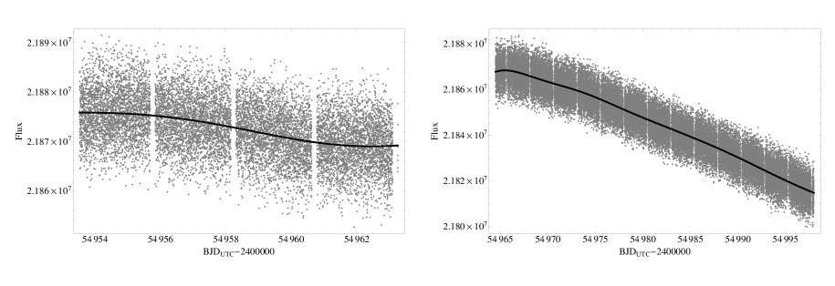
Figure 1.— “Raw” (PA output) flux from DR5 of the Kepler pipeline for Q0 (left panel) and Q1 (right panel) of the star TrES-2. Overlaid is our model for the long-term trend, computed using a discrete cosine transform for each data set. Outliers have been removed.

2.3. Median Normalizations

A second stage of normalization is applied to the data after the long-term detrending. Here, we split the lightcurve up into 18 individual transit and occultation events (giving 36 arrays in total). Each array spans from -0.125 to +0.125 in orbital phase surrounding the event in question. The fluxes and associated errors in each array and then divided by the median of each array. This is similar to the technique adopted by Kipping & Bakos (2010).

2.4. Outliers

Despite the PA processing, some outliers still remain in our detrended, normalized photometry. We must remove these before it is possible to perform the final lightcurve fits. Since these outliers can occur within the transit event itself, it is necessary to perform a preliminary fit of the transits and then remove outliers from the residuals.

For the purpose of the identifying outliers, we perform an initial global fit (as described later in § 3.2). The residuals are then used to search for outlier points by flagging those which occur 3-$\sigma$ away from the model.

2.5. Time Stamps

In the DR5 handbook, the following advise is given:

“The advice of the DAWG [Data Analysis Working Group] is not to consider as scientifically significant relative timing variations less than the read time (0.5s) or absolute timing accuracy better than one frame time (6.5s) until such time as the stability and accuracy of time stamps can be documented to near the theoretical limit.”

Relative time differences correspond to, for example, performing TTV (transit timing variations) and TDV (transit duration variations) on the Kepler data alone. Absolute time differences corresponds to, for example, performing TTV and TDV on the Kepler data plus all previously observed data. We stress these limitations early on in our study.

The Kepler time stamps from DR5 are in BJD_UTC (Barycentric Julian Date in Coordinated Universal Time) and a correction to $\mathrm{BJD}_{\mathrm{TDB}}$ (Barycentric Julian Date in Terrestrial Dynamic Time) is advocated by Eastman et al. (2010) in all transit timing studies. The correction between UTC and TDB is given by $\mathrm{BJD}_{\mathrm{TDB}}=\mathrm{BJD}_{\mathrm{UTC}}+N+32.184$, where $N$ is the number of leap seconds which have elapsed since 1961. This correction has been applied all data analyzed in this study.

2.6. Correlated Noise

Time-correlated noise may affect the estimation of lightcurve parameters (Carter et al., 2010) and so we here discuss the degree to which this data set is affected by correlated noise. We present two methods of assessing the degree of red noise, following the approach adopted by Carter et al. (2009).

First, using the residuals of our final fits (which will be introduced in more detail in §3.2), we bin the residuals into a bin size $N$ and evaluate the r.m.s. of the data. We repeat this process from $N=1$ up to $N=360$ (which is approximately equal to the time span of each discrete lightcurve array, 0.25 days) and the results are shown in Figure 2. The figure reveals that our corrected data is follows closely the expectation of independent random numbers, $\sigma_{N}=\sigma_{1}N^{-1/2}[M/(M-1)]^{1/2}$, where $M$ is the number of bins.

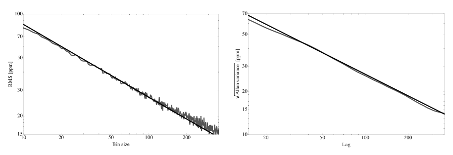
Figure 2.— Assessment of correlated noise. Left panel: The r.m.s. of the time-binned residuals as function of bin-size. Right panel: The square-root of the Allan variance of the residuals, as a function of lag. The gray lines are computed from the data and the black lines show the expected behavior for uncorrelated noise.

Second, we computed the Allan (1966) variance $\sigma_{A}^{2}(l)$ of the residuals, defined as:

$$\sigma_{A}^{2}(l)=\frac{1}{2(N+1-2l)}\sum_{i=0}^{N-2l}\Bigg{(}\frac{1}{l}\sum_{j=0}^{l-1}r_{i+j}-r_{i+j+l}\Bigg{)}^{2}$$ (3)

where $r_{k}$ denotes the residual of the $k^{\mathrm{th}}$ data points, $N$ is the number of data points and $l$ is the lag. For independent residuals, one expects $\sigma_{A}^{2}(l)\simeq\sigma_{A}^{2}(0)/l$, for which our residuals can be seen to be satisfy in Figure 2.

The bulk r.m.s. of our data set is 237.2 ppm. In comparison, the PCD corrected photometry has a bulk r.m.s. of 230.5 ppm (after removing outliers). It is possible that PCD overfitted the data or that our own correction is an underfit. Based upon the analysis above though, we find no strong evidence for correlated noise in our corrected photometry, which would be expected for underfitted detrending.

3. MODEL DETAILS

3.1. Model Generation

3.1.1 Lightcurves

The primary transit lightcurve model is computed using the Mandel & Agol (2002) limb darkening algorithm. The outputted fluxes are corrected for variable baseline flux, OOT, to propagate the baseline r.m.s. into the lightcurve. The occultation lightcurve is computed in the same way, except the limb darkening coefficients are fixed to zero and the final lightcurve is then squashed by a factor which is equal to the ratio of the transit to occultation depth. We note that multiplying the ratio-of-radii squared, $p^{2}$, by this factor and then feeding this value into the Mandel & Agol (2002) code instead would be erroneous, since the algorithm would think the planet was very small leading to sharper ingress/egress features. By applying the transformation at the end, we preserve the correct lightcurve morphology.

The true anomaly is calculated from the time stamps by solving Kepler’s Equation at every instance. Transit durations are computed using the expressions of Kipping (2008), which account for orbital eccentricity. Although TrES-2b is believed to be on a circular orbit (O’Donovan et al., 2007), using the most general equations allows us to float the eccentricity parameters to propagate their uncertainties. Recent Spitzer occultation measurements by O’Donovan et al. (2010) strongly constrain $e\cos\omega=(0.00053\pm 0.00102)$. We allow both $e\sin\omega$ and $e\cos\omega$ to be fitted for in our global fits, but as the $e\cos\omega$ term moves away from the value found by O’Donovan et al. (2010), a $\chi^{2}$ penalty is assigned (see Equation 3.2)

We initially use the errors from the normalized PA lightcurve and then rescale the errors after one iteration of the global fit. Errors are scaled such that the $\chi^{2}$ function for the transit data, the occultation data, the RV data and the transit times are each equal to the number of data points in that fit minus the number of degrees of freedom in the model.

3.1.2 Radial velocity

The radial velocity curve is computed assuming a single planet in a Keplerian orbit. The free parameters in the model are the time of transit, the orbital period, $e\cos\omega$, $e\sin\omega$ and the semi-amplitude $K$. We do not consider the Rossiter-McLaughlin (RM) effect since our principal goal is to characterize the orbit and the points for the RM lead to very little improvement in the parameters listed here (Winn et al., 2008), but severe increases in CPU time. As a result, we only use the radial velocities from O’Donovan et al. (2007), taking care to convert the times to BJD_TDB.

3.1.3 Transit times

So far we have three data sets which are fitted for; the transits, the occultations and the radial velocities. Usefully, TrES-2b is a relatively old discovery and several years of transit measurements exist. However, most of these come from amateur measurements, which have not been peer-reviewed, and thus may not be as reliable. A resolution to this is to use median statistics to define the merit function and therefore provide a robust estimation of the goodness of fit, even in the presence of outliers. We therefore add in a fourth data set to our global fits coming from the timings, which provides extremely tight constraints on the ephemeris.

Let us consider the typical merit of function first, which is based on mean statistics. In order to compute the ephemeris, we throw in a trial model of $\tau+nP$ and then calculate the residuals for each point, $r_{i}$. We then evaluate the weighted squares of each of these measurements, given by $(r_{i}/\sigma_{i})^{2}$, where $\sigma_{i}$ is the measurement error. In a normal analysis, we would then sum these weighted squares together to give the $\chi^{2}$ and then perturb the model until we obtain the lowest possible $\chi^{2}$:

$$\chi^{2} =\sum_{i=1}^{n}(r_{i}/\sigma_{i})^{2}$$

$$\chi^{2} =n\,\frac{\sum_{i=1}^{n}(r_{i}/\sigma_{i})^{2}}{n}$$

$$\chi^{2} =n\,\mathrm{Mean}\{(r_{i}/\sigma_{i})^{2}\}$$ (4)

Inspection of the above equation reveals the simple way in which we can change our merit function to be in the form of median statistics, to give “$\xi^{2}$”:

$$\xi^{2}=n\,\mathrm{Median}\{(r_{i}/\sigma_{i})^{2}\}$$ (5)

The $\xi^{2}$ distribution is very similar to that of the $\chi^{2}$ distribution, but a scaling factor is required to make them equivalent. This factor is frequently required when converting median statistics to mean statistics; for example the standard deviation is given by 1.4286 times by the median-absolute-deviation and the error on the sampling median is 1.253 times the error on the sampling mean. In this case, the factor was computed using Monte Carlo simulations where we found the factor $2.2\dot{6}$ provides the correct scaling.

Times of transit minimum found in the exoplanet literature and the ETD (Exoplanet Transit Database) are almost always in HJD_UTC (Heliocentric Julian Date in Coordinated Universal Time). We use the JPL Horizons ephemeris to convert the HJD_UTC times to BJD_UTC and then apply the correction for leap-seconds to yield BJD_TDB. The list of used transit times is presented in the appendix, Table 5.

3.2. Fitting Algorithm

Fits are accomplished by using a Metropolis-Hastings Markov Chain Monte Carlo (MCMC) algorithm (Tegmark et al., 2004; Holman et al., 2006). The routine begins from a starting point, which we select to be 5-$\sigma$ away from the estimated solution, and then generates new trial parameters by making a jump computed using a Gaussian proposal distribution centered upon the current position with a standard deviation given by the “jump size”. Jump sizes are selected, usually through a process of iteration, to be equal to the 1-$\sigma$ uncertainties for each parameter.

The trial parameters are then used to produce a model, which is compared to the observations to produce the goodness-of-fit merit function, $\chi^{2}$. Trials producing a lower $\chi^{2}$ than the current position are always accepted and the trial position becomes the current position, constituting an accepted jump. Trials producing a higher $\chi^{2}$ are accepted with a probability:

$$\mathrm{P}(\mathrm{accept}) =\exp(-\Delta\chi^{2}/2)$$ (6)

where $\Delta\chi^{2}$ is the difference in $\chi^{2}$ between the current position and the trial position. The algorithm stops when 125,000 trials have been accepted and the first 25,000 (20%) are discarded as burn-in leaving $10^{5}$ points for the posterior distributions. Our algorithm follows the same procedure detailed in Ford (2005). The overall merit function (see §3.1 for details) is given by:

$$\chi^{2}= \sum_{i=1}^{n_{P}}\Big{(}\frac{f_{\mathrm{obs},i}^{P}-f_{\mathrm{model},i}^{P}}{\delta f_{i}^{P}}\Big{)}^{2}+\sum_{i=1}^{n_{S}}\Big{(}\frac{f_{\mathrm{obs},i}^{S}-f_{\mathrm{model},i}^{S}}{\delta f_{i}^{S}}\Big{)}^{2}$$

$$+\sum_{i=1}^{n_{R}}\Big{(}\frac{v_{\mathrm{obs},i}-v_{\mathrm{model},i}}{\delta v_{i}}\Big{)}^{2}+\Big{(}\frac{e\cos\omega-0.00053}{0.00102}\Big{)}^{2}$$

$$+2.2\dot{6}n_{T}\mathrm{Median}\Big{\{}\Big{(}\frac{t_{\mathrm{obs},i}-t_{\mathrm{model},i}}{\delta t_{i}}\Big{)}^{2}\Big{\}}$$ (7)

We fit using 14 free parameters {$\tau$, $P$, $p^{2}$, $\tilde{T}_{1}$, $b$, $e\cos\omega$, $e\sin\omega$, OOT, OOS, $w_{1}$, $w_{2}$, $F_{P}/F_{*}$, $K$, $\gamma$}, which we elaborate on here. $\tau$ is the time of transit minimum for the optimum epoch (that epoch which produces the minimum correlation to $P$) and is defined as the instance when the planet-star sky-projected separation is minimized (note, this is frequently given the misnomer “mid-transit time”). $P$ is the orbital period, $p^{2}$ is the ratio-of-radii squared and $b$ is the impact parameter (defined as the planet-star sky-projected separation in units of the stellar radius at the instance of inferior conjunction). $\tilde{T}$ is the transit duration between the instance of the planet’s center crossing the stellar limb to exiting under the same condition. $\tilde{T}_{1}$ is the “one-term” approximate expression for this parameter, given by Equation 15 in Kipping (2010a) (an exact analytic form for $\tilde{T}$ is not possible, see Kipping (2010a) for details). Stellar limb darkening is accounted for using a quadratic limb darkening model, modeling the specific intensity as a function of $\mu$:

$$\frac{I_{\mu}}{I_{1}} =1-u_{1}(1-\mu)-u_{2}(1-\mu)^{2}$$ (8)

where $\mu$ is the cosine of the angle between the observer and the normal to the stellar surface. $u_{1}$ and $u_{2}$ are known to be highly correlated in typical lightcurve fits (Pál, 2008) and instead we opt to use $w_{1}$ and $w_{2}$, which are related to the quadratic limb darkening coefficients (Pál, 2008) via:

$$w_{1} =u_{1}\cos\varphi-u_{2}\sin\varphi$$

$$w_{2} =u_{2}\cos\varphi+u_{1}\sin\varphi$$ (9)

Pál (2008) has advocated using this linear combination instead of $u_{1}$ and $u_{2}$ due to the improved decorrelations. The author also recommends using $\varphi=40^{\circ}$, which was done so in this study. During the MCMC, we discard any trials which yield unphysical limb darkening coefficients, defined as those which are not everywhere positive and produce a monotonically decreasing profile from limb to center. This is implemented by using the conditions (Carter et al., 2009): $u_{1}+u_{2}<1$, $u_{1}+u_{2}>0$ and $u_{1}>0$.

Finally, the final parameter values quoted in this paper are given by the median of all of the accepted MCMC trials for the parameter in question. Similarly, 1-$\sigma$ uncertainties are calculated by evaluating the 34.1% quantiles either side of the median.

3.2.1 Why fit for eccentricity?

Some readers may question why we choose to fit for eccentricity when the orbit is consistent with a circular orbit (O’Donovan et al., 2007). Firstly, we point out that by using all of the known transit times, the Kepler lightcurves and occultation constraints we are able to derive the most precise constraints on $e$ yet for this system, which is a worthwhile goal in itself.

However, the most important reason for fitting for $e$ is that any uncertainty on $e$ leads to inflated uncertainties on the derived stellar density, $\rho_{*}$. As pointed out by Kipping (2010a), the retrieved stellar density is given by the approximation $\rho_{*}\simeq\rho_{*,\mathrm{circ}}/\Psi(e,\omega)$ where the first term is the stellar density derived from a circular fit and $\Psi$ is given by:

$$\Psi=\frac{(1+e\sin\omega)^{3}}{(1+e^{2})^{3/2}}$$ (10)

$\rho_{*,circ}$ is determined purely photometrically and thus the uncertainty will decrease as $\sim 1/\sqrt{N_{\mathrm{transits}}}$, where $N_{\mathrm{transits}}$ is the number of observed transits by Kepler. This parameter can therefore be expected to be known to very high precision by the end of the Kepler Mission, given the short orbital period of TrES-2b. In contrast, $\Psi$ can only be measured by radial velocities and/or occultation events. Given the visible bandpass of Kepler, occultation events are not expected to be detectable for the majority of transiting planets, and so the radial velocity determination dominates. With typical transiting planets receiving sparse radial velocity coverage, it can be appreciated that the uncertainty on $\Psi$ will often be the limiting factor in the measurement of a precise $\rho_{*}$.

The point is that we do not know the orbit is exactly circular (indeed this is practically impossible) and thus we cannot assume $e\sin\omega=0$ and $e\cos\omega=0$ exactly. In reality, we have errors on both of these and can only say it is circular to within a certain confidence level. This uncertainty therefore propagates into a much larger error for the stellar density. As an example, Kipping & Bakos (2010) compare fits for Kepler-4b through 8b using both circular and eccentric fits and find the errors on $\rho_{*}$ consistently inflate for the latter.

3.2.2 Why fit for limb darkening?

Another methodology we adopt, which is not a completely standard practice in the exoplanet literature, is that we fit for the limb darkening coefficients. Fitting for quadratic limb darkening requires a very high signal-to-noise if one wishes to achieve convergence, especially for a near-grazing transit. In many ground-based measurements, it is not possible to fit for these coefficients, although linear limb darkening could be used instead.

However, if fitting for the limb darkening is viable, it is always preferable. This is because transit parameters derived using fixed limb darkening coefficients are fundamentally model dependent, where the model is that of the stellar atmosphere model. In contrast, transit parameters derived using fitted limb darkening are independent of a stellar atmosphere. This makes them vastly more robust and reliable.

This point is particularly salient for TrES-2b. For a near-grazing transit, the planet only ever crosses the limb, where the star is most severely darkened. Thus the choice of limb darkening coefficients has a very significant effect on the derived planetary radius and transit depth especially. The total stellar flux, which defines the observed transit depth, is essentially extrapolated from the stellar centre to the limb based upon the fitted limb darkening coefficients of the limb only. This leads to large correlations between the limb darkening coefficients and the ratio-of-radii squared.

3.3. Blending

Recently, Daemgen et al. (2009) showed that the TrES-2 has a very nearby star, which was proposed to be in binary star system composed of the originally known G0 TrES-2A star and a previously undetected K4.5-K6 companion, (labeled TrES2/C by the authors). In the z’-band, the magnitude difference was estimated to be 3.43 and thus we estimate the blending factor $B$ (which is defined in Kipping & Tinetti (2010)) to be $B=(1.04246\pm 0.00023)$.

This blending acts to dilute the transit depth and thus causes us to underestimate the true planetary radius. Correcting for blends may be accomplished by following the prescription of Kipping & Tinetti (2010), which we adhere to in this work. Self-blending due to nightside emission is expected to be negligible in the Kepler bandpass (see same work) and thus need not be accounted for.

3.4. Limb Darkening Computation

In §4.1, we will discuss how limb darkening coefficients are fitted for in the final results. However, it is useful to generate the limb darkening coefficients from theoretical models for i) providing a sensible starting point for the fitting procedure ii) later comparison of theoretical models versus fitted limb darkening.

Limb darkening coefficients were calculated for the Kepler bandpass for TrES-2b. For the Kepler bandpass, we used the high resolution Kepler transmission function found at http://keplergo.arc.nasa.gov/CalibrationResponse.shtml. We adopted the SME-derived stellar properties reported in Sozzetti et al. (2007). We employed the Kurucz (2006) atmosphere model database providing intensities at 17 emergent angles, which we interpolated linearly at the adopted $T_{\mathrm{eff}}$ and $\log g$ values. The passband-convolved intensities at each of the emergent angles were calculated following the procedure in Claret (2000). To compute the coefficients we used the limb darkening law given in Equation 8.

The final coefficients resulted from a least squares singular value decomposition fit to 11 of the 17 available emergent angles. The reason to eliminate 6 of the angles is avoiding excessive weight on the stellar limb by using a uniform sampling (10 $\mu$ values from 0.1 to 1, plus $\mu=0.05$), as suggested by Díaz-Cordovés et al. (1995).

3.5. Drifts and Trojans

Before we provide the final results, we discuss how we performed global fits including a linear drift in the radial velocities, $\dot{\gamma}$, and a temporal offset between the radial velocity null and the time of transit minimum, $\Delta t$ (such a temporal offset is expected to be induced by Trojans (Ford & Gaudi, 2006)). By switching on and off these parameters, there are four possible permutations of the fits we can execute; eight when one switches on/off eccentricity as well (see Table 1).

In general, fitting for an excessive number of free parameters is undesirable as it increases the errors on the other terms. In order to decide whether these two additional parameters should be included or not, one may evaluate the Bayesian Information Criterion (BIC) (Schwarz, 1978; Liddle et al., 2007), for each of the proposed models. The model with the lowest BIC is accepted and subsequently used in the global fits reported in the next section. These fits used 125,000 MCMC trials with a more aggressive $\chi^{2}$ minimization downhill simplex implemented afterwards. It is based on this lowest $\chi^{2}$ solution from which the BIC is computed.

We therefore performed eight versions of our global fits, with the results for the BIC values presented in Table 1. We find that neither a drift nor a temporal offset are accepted for either the circular or eccentric models. We therefore proceed to consider them fixed to zero. The results, however, do allow us to place upper limits on $\dot{\gamma}$ and $\Delta t$. We find $|\dot{\gamma}|<0.12$ $\mathrm{m}\mathrm{s}^{-1}\mathrm{year}^{-1}$ and $|\Delta t|<0.15$ days to 3-$\sigma$ confidence. This excludes a $>0.94$ $M_{J}$ Trojan in a 1:1 resonance with TrES-2b.

Table 1Bayesian Information Criterion (BIC) values for eight models executed for the global fits. We highlight the lowest BIC values.

Model	BIC
$e=0$,$|\dot{\gamma}|=0$,$|\Delta t|=0$	34048.7
$e=0$,$|\dot{\gamma}|>0$,$|\Delta t|=0$	34064.2
$e=0$,$|\dot{\gamma}|=0$,$|\Delta t|>0$	34058.6
$e=0$,$|\dot{\gamma}|>0$,$|\Delta t|>0$	34069.7
$e>0$,$|\dot{\gamma}|=0$,$|\Delta t|=0$	34067.2
$e>0$,$|\dot{\gamma}|>0$,$|\Delta t|=0$	34077.5
$e>0$,$|\dot{\gamma}|=0$,$|\Delta t|>0$	34259.1
$e>0$,$|\dot{\gamma}|>0$,$|\Delta t|>0$	34268.4

4. RESULTS OF GLOBAL FITS

Table 2Results from global fits of TrES-2b using eighteen short-cadence (SC) Kepler transits. We show results for both circular and eccentric fits in columns 2 and 3. In column 4, we provide the previous estimates of the system parameters from O’Donovan et al. (2007)ⁱ Holman et al. (2007)ⁱⁱ and Sozzetti et al. (2007)ⁱⁱⁱ. In general, the eccentric fit leads to more realistic errors. Quoted values are medians of MCMC trials with errors given by 1-$\sigma$ quantiles. * = fixed parameter; $\dagger$ = parameter was floated but not fitted.

Parameter	Circular	Eccentric	Previous
Model indep. params.
$P$ [days]	$2.47061896_{-0.00000016}^{+0.00000022}$	$2.47061892_{-0.00000012}^{+0.00000018}$	$2.470621\pm 0.000017$ ii
$\tau$ [BJDTDB - 2,450,000]	$4849.526635_{-0.000026}^{+0.000026}$	$4849.526640_{-0.000021}^{+0.000022}$	-
$T_{1,4}$ [s]	$6438_{-33}^{+31}$	$6439_{-28}^{+25}$	$6624\pm 72$ ii
$\tilde{T}_{1}$ [s]	$4624_{-41}^{+42}$	$4624_{-31}^{+32}$	-
$T_{2,3}$ [s]	$1950_{-110}^{+110}$	$1942_{-86}^{+84}$	-
$(T_{1,2}\simeq T_{3,4})$ [s]	$2242_{-47}^{+49}$	$2247_{-37}^{+38}$	$2459\pm 162$ ii
$(R_{P}/R_{*})^{2}$ [%]	$1.643_{-0.052}^{+0.082}$	$1.633_{-0.045}^{+0.076}$	-
$b$	$0.8408_{-0.0053}^{+0.0047}$	$0.8418_{-0.0045}^{+0.0037}$	$0.8540\pm 0.0062$ ii
$\delta_{\mathrm{occultation}}$ [ppm]	$21_{-22}^{+23}$	$19_{-17}^{+18}$	-
$e\sin\omega$	$0^{\mathrm{*}}$	$-0.009_{-0.029}^{+0.024}$	$0^{\mathrm{*}}$ ii
$e\cos\omega$	$0^{\mathrm{*}}$	$0.0005_{-0.0018}^{+0.0018}$	$0^{\mathrm{*}}$
$\Psi$	$1^{\mathrm{*}}$	$0.973_{-0.082}^{+0.071}$	$1^{\mathrm{*}}$ ii
$K$ [ms-1]	$181.4_{-6.7}^{+6.8}$	$181.0_{-5.4}^{+5.5}$	$181.3\pm 2.6$ i
$\gamma$ [ms-1]	$-29.9_{-5.6}^{+5.6}$	$-29.2_{-2.6}^{+2.6}$	-
$B$	$1.04246\pm 0.00023$ $\dagger$	$1.04246\pm 0.00023$ $\dagger$	$1^{*}$ ii
$u_{1}$	$0.52_{-0.34}^{+0.44}$	$0.45_{-0.30}^{+0.42}$	$0.22^{*}$ ii
$u_{2}$	$0.06_{-0.48}^{+0.37}$	$0.12_{-0.46}^{+0.33}$	$0.32^{*}$ ii
$R_{P}/R_{*}$	$0.1282_{-0.0020}^{+0.0032}$	$0.1278_{-0.0018}^{+0.0029}$	$0.1253\pm 0.0010$ ii
$a/R_{*}$	$7.983_{-0.084}^{+0.132}$	$8.06_{-0.21}^{+0.25}$	$7.63\pm 0.12$ ii
$i$ [∘]	$83.952_{-0.094}^{+0.131}$	$84.07_{-0.31}^{+0.34}$	$83.57\pm 0.14$ ii
$e$	$0^{\mathrm{*}}$	$0.018_{-0.013}^{+0.023}$	$0^{\mathrm{*}}$ ii
$\omega$ [∘]	-	$268_{-180}^{+7}$	- ii
$\rho_{*}$ [g/,cm-3]	$1.63_{-0.13}^{+0.16}$	$1.63_{-0.13}^{+0.16}$	$1.375\pm 0.065$ iii
$\log(g_{P}\,[\mathrm{cgs}])$	$3.317_{-0.018}^{+0.018}$	$3.326_{-0.024}^{+0.025}$	-
Model depend. params.
$T_{\mathrm{eff}}$ [K] (SME)	$5850\pm 50$ $\dagger$	$5850\pm 50$ $\dagger$	$5850\pm 50$ iii
$\log(g\,[\mathrm{cgs}])$ (SME)	$4.4\pm 0.1$ $\dagger$	$4.4\pm 0.1$ $\dagger$	$4.4\pm 0.1$ iii
(Fe/H) [dex] (SME)	$-0.15\pm 0.10$ $\dagger$	$-0.15\pm 0.10$ $\dagger$	$-0.15\pm 0.10$ iii
$M_{*}$ [$M_{\odot}$]	$0.992_{-0.050}^{+0.040}$	$0.990_{-0.048}^{+0.041}$	$0.980\pm 0.062$ iii
$R_{*}$ [$R_{\odot}$]	$0.958_{-0.020}^{+0.018}$	$0.952_{-0.029}^{+0.028}$	$1.000_{-0.033}^{+0.036}$ iii
$\log(g\,[\mathrm{cgs}])$	$4.469_{-0.012}^{+0.015}$	$4.475_{-0.024}^{+0.024}$	$4.426_{-0.023}^{+0.021}$ iii
$L_{*}$ [$L_{\odot}$]	$0.961_{-0.057}^{+0.058}$	$0.948_{-0.070}^{+0.073}$	-
$M_{V}$ [mag]	$4.877_{-0.072}^{+0.074}$	$4.892_{-0.088}^{+0.090}$	$4.77\pm 0.09$ iii
Age [Gyr]	$3.3_{-1.3}^{+1.9}$	$3.1_{-1.6}^{+2.0}$	$5.1_{-2.3}^{+2.7}$ iii
Distance [pc]	$202.6_{-6.8}^{+6.8}$	$201.2_{-8.2}^{+8.3}$	$220\pm 10$ iii
$M_{P}$ [$M_{J}$]	$1.205_{-0.058}^{+0.058}$	$1.202_{-0.051}^{+0.050}$	$1.198\pm 0.053$ ii
$R_{P}$ [$R_{J}$]	$1.199_{-0.022}^{+0.020}$	$1.187_{-0.035}^{+0.034}$	$1.222\pm 0.038$ ii
$\rho_{P}$ [g cm-3]	$0.870_{-0.041}^{+0.042}$	$0.891_{-0.064}^{+0.074}$	-
$a$ [AU]	$0.03566_{-0.00062}^{+0.00048}$	$0.03563_{-0.00058}^{+0.00048}$	$0.0367_{-0.0005}^{+0.0012}$ i

The global fits were performed using the full Kepler time series as described in §3.1. The final results are given in Table 2. After the main MCMC fits, a downhill simplex routine is used to obtain the lowest $\chi^{2}$ solution. We plot this solution over the data in Figure 3. Histograms of the marginalized posterior distributions for each of the fitted parameters are shown in Figure 4, which clearly indicate convergence of the fitting parameters.

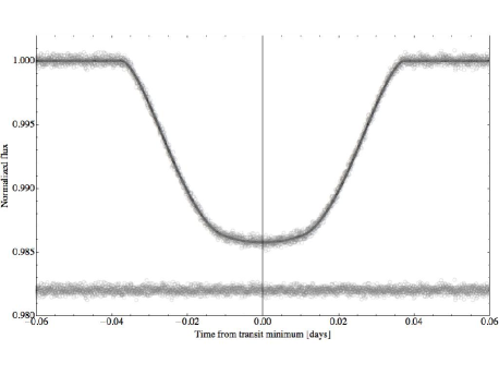
Figure 3.— Short-cadence folded transit lightcurve of TrES-2b (circles) with model fit overlaid. Residuals from the fit are shown below, offset by +0.982.

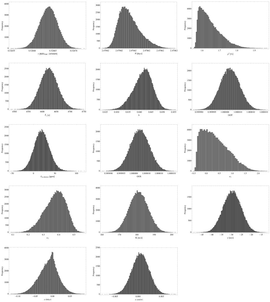
Figure 4.— Marginalized parameter posterior distributions. Reading down from top left to right, we have $\tau$, $P$, $p^{2}$, $\tilde{T}_{1}$, $b$, OOT, $\delta_{\mathrm{occultation}}$, OOS, $w_{1}$, $w_{2}$, $K$, $\gamma$, $e\sin\omega$ and $e\cos\omega$. Results come from global fits assuming no Trojan body and no linear drift in the RVs, but allowing orbital eccentricity.

4.1. Limb Darkening Fitting

Fitting for the limb darkening (LD) coefficients is challenging because TrES-2b is a near-grazing transit and thus only samples a fraction of the stellar surface. However, the extremely high quality of the Kepler SC photometry and the fact we have 18 transits does allow for a good solution (given in Table 2). The inevitably strong correlations between the quadratic coefficients is presented in Figure 5.

We find that the theoretical limb darkening coefficients lie within the 1-$\sigma$ confidence region of our fits, indicating an impressive prediction for the Kurucz (2006) atmosphere model. One major benefit of fitting for the limb darkening is that the uncertainty in the stellar properties is built into the model and thus leads to larger, and ultimately more realistic, estimates of the various parameter uncertainties. Parameters which are highly correlated to the limb darkening coefficients, such as the the transit depth (see §3.2.2), have their associated errors increase considerably as a result of this process.

As discussed in §3.2, we actually fitted for $w_{1}$ and $w_{2}$ rather than $u_{1}$ and $u_{2}$ to decrease the correlations, following the prescription of Pál (2008). We chose $\varphi=40^{\circ}$, as this was suggested as a useful first-guess for the term by Pál (2008). However, future studies of this system would benefit by using a more optimized value of $\varphi$. By using a principal component analysis (PCA), we are able to find this optimum angle to be $\varphi=42.7033^{\circ}$, very close to the $35^{\circ}-40^{\circ}$ range advocated by Pál (2008).

It is important to consider the effects of fitting for LD carefully. We re-ran our fits with the LD parameters fixed to their best-value and found that the errors on numerous parameters were considerably reduced, in many cases by an order-of-magnitude. As an example, the transit depth error is reduced by a factor of 17.5 when we fixed the LD parameters. The errors found using fitted LD correspond to the absolute uncertainty in each parameter. Therefore, if we wish to compare the duration found from Kepler photometry with, say, a ground-based measurement in a different bandpass, we must fit for the LD parameters separately in both cases. However, if we consistently employ the same bandpass and instrument response function for the same star, then there is no need to refit the LD parameters everytime. By fixing the LD parameters to their best-value, we compute the relative duration changes, within that bandpass.

For TTV, the error in the time of transit minimum does not appreciably change between fitting and not-fitting the LD parameters. Therefore, the TTV seems to be reliable across different bandpasses and instruments. This opportunity will be exploited later in §7.

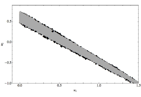
Figure 5.— Distribution of the quadratic limb darkening coefficients from the MCMC global fits of the short-cadence data. Black points correspond to the 3-$\sigma$ region and gray to the 1-$\sigma$. The diamond marks the theoretical limb darkening coefficients computed from a Kurucz (2006) style atmosphere.

4.2. Occultation

In the short cadence global fits, we do not detect an occultation for the planet in the circular nor the eccentric fits. Although no occultation is detected, a robust upper limit is obtained. We choose to use the eccentric fit from here on, as it provides the most realistic errors (see §3.2.1).

The best-fitted occultation depth is $\delta_{\mathrm{occultation}}=19_{-17}^{+18}$ ppm, indicating no detected signal. The posterior distribution of the occultation depth is presented in Figure 4. We exclude an occultation of depth $>72.9$ ppm to $3$-$\sigma$ confidence.

Recently, Spiegel & Burrows (2010) predicted that the occultation of TrES-2b, in Kepler’s bandpass, would be $\leq 20$ ppm, assuming no reflected light contribution. Our results are therefore highly consistent with the theoretical models for this planet.

The 3-$\sigma$ limit constrains the geometric albedo to be $A_{g}<0.146$ and a dayside brightness temperature of $T_{P,day}<2413$ K (for comparison, the equilibrium temperature is 1472 K). We note that our 3-$\sigma$ limit is tighter than that for HD 209458b as measured by Rowe et al. (2008) using MOST, where $A_{g}<0.17$ to $3$-$\sigma$ confidence. Therefore, TrES-2b is currently the darkest exoplanet known to exist. For comparison, the upper limit corresponds to a planet of similar albedo to Mercury (0.138).

4.3. A Search for Asymmetry

Lightcurve asymmetry is generally not expected but may reveal interesting, new physics for hot-Jupiters. One possible source would be an oblate star with a significant spin-orbit misalignment causing an asymmetry in the ingress/egress durations. We here describe how we searched for asymmetry in the lightcurve.

We divide the folded lightcurve into points before and after the globally fitted time of transit minimum, where the fold is performed using the globally fitted period. We then mirror the two halves upon each other to search for signs of asymmetry in the lightcurve. The residuals of these two halves are shown in Figure 6.

We first perform a linear interpolation of the folded data prior to the time of transit minimum. This function is then evaluated at the time stamps of the folded data after the time of transit minimum and the associated uncertainties are carried over. We then subtract the two and add the two sets of flux uncertainties in quadrature. The “mirror residue” exhibits an r.m.s. scatter of 305 ppm, whereas from a theoretical point-of-view one expects scatter equal to $\sqrt{2}\times 237.2$ ppm = $335$ ppm. A chi squared test gives 6990 for 7684 data points. The ingress and egress therefore exhibit remarkable symmetry.

The most significant feature in Figure 6 is a slight drop at around +0.02 days. This feature is only 2-$\sigma$ significant with the current data, but could be scrutinized further in later data releases.

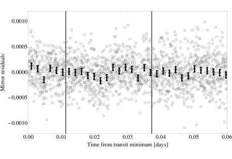
Figure 6.— Mirror residuals. Subtracting the two halves of the lightcurve from each other produces the “mirror” residuals, which would reveal any signs of lightcurve asymmetry - however, none are evident. The vertical black lines mark the start of ingress/egress and the end of ingress/egress.

4.4. Eccentricity

As shown in Table 2, we performed both circular and eccentric fits to illustrate the consequences of fitting for eccentricity. The fits find very similar $\chi^{2}$ values, with the circular fit being marginally larger by $\Delta\chi^{2}=1.89$ for 30697 data points. Using an F-test, we find that the eccentric fit is accepted over the circular fit with a confidence of 38.9%, which we consider to be insignificant. Therefore, we conclude the orbit of TrES-2b is consistent with a circular orbit, based upon the current data. Further, using the marginalized posterior distribution, we estimate that the eccentricity satisfies $e<0.094$ to 3-$\sigma$ confidence.

The $e\cos\omega$ prior from O’Donovan et al. (2010) places a much stronger constraint than that obtained for either component purely from the radial velocity. As a result, we find a much larger uncertainty on $e\sin\omega$ than $e\cos\omega$. Whilst both components are consistent with zero, it is unlikely from an a-priori perspective than $e\sin\omega$ will be non-zero given that $e\cos\omega$ is essentially zero. If both components had similar uncertainties, but consistent with zero, then the eccentricity would be tied down to $e<0.0085$, but we stress that this is not a conclusion which can supported purely based upon the data.

4.5. Revised Masses and Radii

Fundamental parameters of the host star such as the mass ($M_{*}$) and radius ($R_{*}$), which are needed to infer the planetary properties, depend strongly on other stellar quantities that can be derived spectroscopically. For this we used the spectroscopic analysis of Sozzetti et al. (2007) who determine $T_{\mathrm{eff}}=(5850\pm 50)$ K, [Fe/H]$=(-0.15\pm 0.10)$ and $\log(g\,[\mathrm{cgs}])=(4.4\pm 0.1)$.

In principle the effective temperature and metallicity, along with the surface gravity taken as a luminosity indicator, could be used as constraints to infer the stellar mass and radius by comparison with stellar evolution models.

For planetary transits a stronger constraint is often provided by the $a/R_{*}$ normalized semi-major axis, which is closely related to $\rho_{*}$, the mean stellar density. The quantity $a/R_{*}$ can be derived directly from the transit lightcurve (Seager & Mallén-Ornelas, 2003) and the RV data (for eccentric cases, see Kipping (2010a)). The results of our 100,000 MCMC trials are used to produce an array of 100,000 estimates for $\rho_{*}$, $T_{\mathrm{eff}}$ and [Fe/H]. For every trial, we match stellar evolution isochrones from Yi et al. (2001) to the observed properties to produce 100,000 estimates of the absolute dimensions of the star. Finally, the planetary parameters and their uncertainties were derived by the direct combination of the posterior distributions of the lightcurve, RV and stellar parameters.

After the first iteration for determining the stellar properties, as described in Bakos et al. (2009), we find that the surface gravity, $\log(g\,[\mathrm{cgs}])=4.475_{-0.024}^{+0.024}$, is highly consistent with the Sozzetti et al. (2007) analysis. Therefore, a second iteration (which would use the new $\log g$ value) of the isochrones was not required and we adopted the values stated above as the final atmospheric properties of the star (shown in Table 2).

The revised parameters are in excellent agreement with the estimates from O’Donovan et al. (2007), Holman et al. (2007) and Sozzetti et al. (2007), all shown in Table 2 for comparison. However, our derived stellar density is markedly larger and this leads to a slightly smaller, more massive star, which consequently ‘deflates’ TrES-2b slightly.

5. TRANSIT TIMING VARIATIONS (TTV)

We will here only consider short-term transit timing variations, which we define to be those occurring within the timescales of the eighteen observed Kepler transits in Q0 and Q1. A long-term transit timing analysis is provided in §7.

5.1. Fitting Method

For the individual fits, we do not expect limb darkening to vary from transit to transit and thus using a single, common set of LD coefficients is justified (as explained earlier in §LABEL:subsub:whyLD). We therefore fix the quadratic coefficients to those found to give the lowest $\chi^{2}$ in the global fit we performed earlier (selected values were $w_{1}=0.22366$ and $w_{2}=0.39288$). Aside from the limb darkening, the eccentricity terms $e\sin\omega$ and $e\cos\omega$ are also held fixed to the lowest $\chi^{2}$ solution ($e\sin\omega=-0.020864$ and $e\cos\omega=0.00076088$). In total, there are five free parameters used: $\{\tau,p^{2},\tilde{T}_{1},b,\mathrm{OOT}\}$. An initial run is used to compute scaling factors individually for each transit epoch, which span $\pm 0.125P$ of the linear ephemeris predictions. The scaling factors are selected so that the lowest $\chi^{2}$ solution found is equal to the number of degrees of freedom in the model, as before.

The individually fitted transit lightcurves are shown in Figure 7 and the parameters in Table 3. We note that in none of the transits is a second transit-like feature observed, as claimed by Raetz et al. (2009).

Figure 7.— Individual transits of TrES-2b from Q0 and Q1 Kepler photometry. Top lightcurve is Kepler epoch 0 going sequentially in time to epoch 18 at the bottom. Residuals are shown below.

5.2. Control Data

We describe here how we produce control data in the form of artificial lightcurves. The act of producing control data by which to compare the genuine observations is a practice frequently applied in many aspects of scientific study. In our case, the control data serves two principal functions:

1. Rescaling of the parameter uncertainties

2. Identification of signals due to “phasing”

5.2.1 Rescaling

Both of these issues were first noted in Kipping & Bakos (2010), although control data was not used. The rescaling issue was observed by the authors as they found that the errors produced by the Metropolis-Hastings MCMC method led to scatters in their TTV and TDV much lower than the parameter uncertainties. The chance of this occurring by coincidence in an isolated case was estimated to be $\sim$10%, however the pattern was recurring for the majority of parameters evaluated. This led the authors to conclude that there was strong evidence the measurement uncertainties were being overestimated.

Calculating the necessary rescaling factor can be achieved by generating control data. For a single global fit, as performed earlier, this would be too time consuming with the 30,000+ data points plus the correlations between limb darkening and depths taking several weeks to fit in a single run. Therefore, the uncertainties presented in Table 2 may in fact be overestimates as well, although we have not confirmed this. For the individual data, one may take advantage of the fact that a planet exhibiting no TTV, TDV, T$\delta$V (depth variations), TbV (impact parameter variations) or baseline variations should yield a $\chi^{2}$ equal to the number of degrees of freedom in each case. For example, for the TDV, we have 18 transits with one model parameter, the mean duration, and so we expect $\chi^{2}=17$.

Since no real system can be assumed to be absolutely temporally invariant, the only practical way forward is to generate artificial data for the control. To accomplish this, we take the global fit model found earlier and sample it at the exact time stamps in each individual transit epoch array. The global model implicitly assumes that no parameters vary from epoch to epoch, satisfying our control condition. Next, we introduce Gaussian noise into the lightcurve equal to the actual noise recorded at those time stamps. This noise includes the scaling factors found in the individual fits, to ensure equivalence. These control lightcurves are then fitting using the Metropolis-Hastings MCMC method using identical starting positions, jump sizes, etc as the individual fits.

The various parameter variations are then evaluated and the necessary scaling factor is computed. The scaling factors are given in the last line of Table 3. Our results agree with the conclusions of Kipping & Bakos (2010) i.e. that all parameters have overestimated errors by around a factor of $\sim 2$. The reason for this overestimation is unclear and despite close examination of our routines, we can find no obvious reason why this should occur. An independent code used for HATNet discoveries (Bakos et al., 2009), which also uses Metropolis-Hastings MCMC, finds very similar uncertainties to the algorithm used in this work (detailed comparisons of the two methods have been previously provided in Kipping & Bakos (2010) and Kipping et al. (2011)), suggesting this is not a specific flaw in our routine.

5.2.2 Phasing

In Kipping & Bakos (2010), the authors considered a new term which they labeled as the transit “phasing”. This corresponds to the time difference between the expected time of transit minimum and the nearest data point. For example, for data of cadence 60 s, we would expect this time difference to be in the range $\pm 30$ s. Phasing does not seem have a linear correlation to observed parameter variations, but does introduce false periods into the power spectrum of the variations (Kipping & Bakos, 2010). Removing the phasing effects is not currently possible, but we can at least generate the effects which phasing induce to compare to the real data.

By generating our control data with the exact same cadence and time stamps as the data which we fit in the individual transit arrays, we can recover any possible influence the phasing may have on our results. In what follows, figures showing parameter variations always have the real data on the left-hand-side and the control data on the right, so the effects of phasing are most clearly visible.

5.3. Analysis of Variance for TTV

Table 3Transit parameters of TrES-2b from individual fits of the SC data. Kepler epoch 0 is defined as the first transit observed by Kepler. In this data, we fix the limb darkening to the best fit values from the global fit. Therefore, the data can be used to look for relative changes between these 18 transits, but not against previous ground-based measurements of TrES-2b. Errors have not been re-scaled, but the scaling factor is provided on the last line, based upon the analysis of control data.

Kepler Epoch	$\tau$ [BJDTDB - 2,450,000]	$T_{1,4}$ [s]	$(R_{P}/R_{*})^{2}$ [%]	$b$	OOT
0	$4955.763285_{-0.000096}^{+0.000096}$	$6460_{-37}^{+37}$	$1.634_{-0.016}^{+0.016}$	$0.8454_{-0.0037}^{+0.0037}$	$0.999995_{-0.000016}^{+0.000016}$
1	$4958.233958_{-0.000098}^{+0.000098}$	$6447_{-39}^{+39}$	$1.631_{-0.016}^{+0.017}$	$0.8437_{-0.0042}^{+0.0040}$	$0.999996_{-0.000016}^{+0.000017}$
2	$4960.704556_{-0.000095}^{+0.000095}$	$6455_{-36}^{+36}$	$1.628_{-0.015}^{+0.016}$	$0.8444_{-0.0037}^{+0.0036}$	$1.000014_{-0.000016}^{+0.000016}$
3	$4963.175188_{-0.000098}^{+0.000099}$	$6426_{-39}^{+39}$	$1.623_{-0.016}^{+0.016}$	$0.8413_{-0.0041}^{+0.0040}$	$1.000006_{-0.000022}^{+0.000022}$
4	$4965.645708_{-0.000094}^{+0.000095}$	$6431_{-37}^{+37}$	$1.624_{-0.015}^{+0.015}$	$0.8401_{-0.0038}^{+0.0037}$	$1.000004_{-0.000016}^{+0.000016}$
5	$4968.116367_{-0.000093}^{+0.000093}$	$6426_{-37}^{+37}$	$1.624_{-0.015}^{+0.016}$	$0.8397_{-0.0040}^{+0.0039}$	$1.000015_{-0.000016}^{+0.000016}$
6	$4970.587001_{-0.000099}^{+0.000099}$	$6434_{-39}^{+39}$	$1.639_{-0.016}^{+0.017}$	$0.8452_{-0.0040}^{+0.0039}$	$0.999998_{-0.000017}^{+0.000017}$
7	$4973.057600_{-0.000099}^{+0.000100}$	$6469_{-38}^{+39}$	$1.626_{-0.016}^{+0.016}$	$0.8432_{-0.0039}^{+0.0037}$	$1.000010_{-0.000017}^{+0.000017}$
8	$4975.528262_{-0.000103}^{+0.000102}$	$6434_{-41}^{+41}$	$1.621_{-0.017}^{+0.018}$	$0.8400_{-0.0046}^{+0.0044}$	$0.999992_{-0.000017}^{+0.000017}$
9	$4977.998830_{-0.000100}^{+0.000100}$	$6430_{-40}^{+40}$	$1.637_{-0.017}^{+0.017}$	$0.8424_{-0.0043}^{+0.0041}$	$1.000010_{-0.000017}^{+0.000017}$
10	$4980.469389_{-0.000099}^{+0.000098}$	$6426_{-39}^{+40}$	$1.615_{-0.016}^{+0.017}$	$0.8407_{-0.0042}^{+0.0041}$	$0.999989_{-0.000017}^{+0.000017}$
11	$4982.939972_{-0.000102}^{+0.000103}$	$6504_{-41}^{+41}$	$1.631_{-0.017}^{+0.017}$	$0.8445_{-0.0041}^{+0.0040}$	$0.999994_{-0.000017}^{+0.000017}$
12	$4985.410672_{-0.000097}^{+0.000096}$	$6426_{-38}^{+38}$	$1.634_{-0.016}^{+0.016}$	$0.8434_{-0.0039}^{+0.0038}$	$0.999991_{-0.000016}^{+0.000016}$
13	$4987.881247_{-0.000096}^{+0.000097}$	$6403_{-37}^{+37}$	$1.626_{-0.015}^{+0.016}$	$0.8403_{-0.0039}^{+0.0037}$	$0.999991_{-0.000016}^{+0.000016}$
14	$4990.351850_{-0.000098}^{+0.000098}$	$6451_{-39}^{+39}$	$1.631_{-0.017}^{+0.017}$	$0.8427_{-0.0041}^{+0.0040}$	$1.000001_{-0.000016}^{+0.000017}$
15	$4992.822571_{-0.000098}^{+0.000097}$	$6448_{-39}^{+39}$	$1.629_{-0.016}^{+0.017}$	$0.8404_{-0.0042}^{+0.0040}$	$0.999997_{-0.000017}^{+0.000017}$
16	$4995.293071_{-0.000098}^{+0.000099}$	$6462_{-39}^{+39}$	$1.629_{-0.016}^{+0.016}$	$0.8436_{-0.0040}^{+0.0039}$	$1.000016_{-0.000016}^{+0.000016}$
17	$4997.763671_{-0.000103}^{+0.000102}$	$6439_{-40}^{+40}$	$1.623_{-0.017}^{+0.017}$	$0.8398_{-0.0043}^{+0.0042}$	$0.999999_{-0.000019}^{+0.000018}$
Scaling Factor	0.5695	0.6036	0.5044	0.5574	0.5171

The TTV, shown in the top-left panel of Figure 8, exhibits a r.m.s. scatter of 5.16 s, which demonstrates the impressive precision of these Kepler measurements. After rescaling the uncertainties, the scatter in the data is consistent with a linear ephemeris, exhibiting a $\chi^{2}=19.0$ for 16 degrees of freedom. The excess scatter is 1.1-$\sigma$ significant, which we consider below our detection threshold. The unscaled errors yield $\chi^{2}=6.2$ for 16 degrees of freedom, supporting the hypothesis that the errors are significantly underestimated and justifying our rescaling methodology. Figure 8 shows the results.

Figure 8.— TTVs of TrES-2b. Top left: Observed TTVs for TrES-2b using the ephemeris of the global fit. Bottom left: F-test periodogram of the observed TTVs. Top right: TTVs computed from control data (artificial lightcurves). Bottom right: F-test periodogram of the control TTVs.

5.4. F-test Periodogram for TTV

The F-test periodogram fits sinusoidal waveforms through the data of various periods, stepping through from the Nyquist frequency to the observational window in equally spaced steps of size 1/1000 of an epoch. Fitting for amplitude and phase, the $\chi^{2}$ is computed in each step, and then the F-test is performed. The false-alarm-probabilities (FAP) of these F-tests are then plotted in a periodogram. It is important to appreciate that the F-test is designed to look for sinusoidal waveforms, and thus periodic but non-sinusoidal waveforms would have their significances attenuated.

The control data reveals periodogram peaks at 2, 4 and 8 cycles which are harmonics of the sampling cadence of one transit measurement per transit epoch. In the real data, only one peak surpasses 95% confidence occurring at a period longer than the observation window. Such long period peaks cannot be considered genuine unless further transit epochs confirm the periodicity. In conclusion, there is no evidence for a TTV signal in the Kepler Q0 and Q1 TrES-2b photometry.

5.5. Excluded TTV Signals

We conclude our analysis of the TTV by evaluating the constraints on other planets, moons and Trojans in the system. For 16 degrees of freedom, r.m.s. scatter producing a $\chi^{2}=36.2$ is excluded to 3-$\sigma$ confidence. This excludes r.m.s. scatter of 7.11 s to the same confidence level.

An outer perturbing planet in a $j$:$j+1$ mean motion resonance (MMR) would cause the inner transiting planet to librate leading to TTVs (Holman & Murray, 2005; Agol et al., 2005). For 1:2, 1:3 and 1:4 resonances, the libration periods are 18.1, 10.5 and 7.2 cycles respectively. We therefore possess sufficient baseline to look for all such resonant planets. This excludes the presence of coplanar, MMR planets in these resonances of 0.11 $M_{\oplus}$, 0.17 $M_{\oplus}$ and 0.22 $M_{\oplus}$ respectively.

For an extrasolar moon in a retrograde orbit, the maximum dynamically stable orbital separation is 0.9309 Hill radii (Domingos et al., 2006). For such a body on a circular, coaligned orbit, we are able to exclude moons of 1.15 $M_{\oplus}$. As the orbital separation decreases, we are able to exclude moons of masses $\geq(1.07/f)\sin i_{s}$ $M_{\oplus}$, where $f$ is equal to the moon’s orbital separation in units of Hill radii.

Trojan bodies can also induce TTVs and thus constraints on their presence can be also established. Using Equation 1 of Ford & Holman (2007), and assuming a Trojan of angular displacement $\sim 10^{\circ}$ from the Lagrange point, we are sensitive to Trojans of cumulative mass $>0.46$ $M_{\oplus}$ to 3-$\sigma$ confidence. However, the expected libration period would be $\sim 75$ cycles and thus we do not yet possess sufficient baseline to definitively exclude such bodies.

5.6. Proposed 0.21 Cycle Period Signal

Another signal we are able to investigate is the one proposed by Rabus et al. (2009). The authors claimed a 0.21 cycle period sinusoid of amplitude 50 s provided a best-fit to the previously known transit times of TrES-2b, with a FAP of 1.1% and suggested a 52 $M_{\oplus}$ exomoon as a possible origin.

Fixing the amplitude and period to the proposed value and fitting for the phase term, we find a $\chi^{2}=1610$ for the 18 data points. In contrast, the static model obtains a $\chi^{2}=19.0$, which therefore excludes the claimed signal to high confidence. This highlights the dangers of looking for signals below the Nyquist frequency.

6. TRANSIT DURATION VARIATIONS (TDV)

6.1. Choosing a Statistic

Due to the near-grazing nature of the transit, the standard assumption that $\tilde{T}$ is the optimum statistic for TDV searches may not be valid (Carter et al., 2008; Kipping, 2009). In particular, the first-to-fourth contact duration, $T_{1,4}$, could potentially offer greater sensitivity. We found that the typical error on $T_{1,4}$ was 0.28% in the individual fits, whereas $\tilde{T}_{1}$ marginally better at 0.24%. Another factor in choosing a statistic comes from the effects of limb darkening. Whilst here we fix the limb darkening coefficients to the best-fit values from the global MCMC, it is preferable to still avoid using a statistic which is strongly correlated to limb darkening. This is because we may be using slightly incorrect limb darkening coefficients which therefore feed into incorrect duration estimations. Whilst this is generally unavoidable, strongly correlated terms would clearly excerbate the situation. We find that $T_{1,4}$ has a correlation of 0.021 to the limb darkening coefficient $w_{2}$ (the most strongly constrained coefficient) whereas $\tilde{T}_{1}$ has a correlation coefficient of 0.81. On this basis, we choose to use the $T_{1,4}$ statistic in what follows, defining the TDV of the $i^{\mathrm{th}}$ transit measurement as:

$$\mathrm{TDV}_{i}=[T_{1,4}]_{i}-[T_{1,4}]_{\mathrm{global}}$$ (11)

6.2. Analysis of Variance for TDV

The TDV, shown in the top-left panel of Figure 9, exhibits a r.m.s. scatter of 22.4 s. After rescaling the uncertainties, the scatter in the data is consistent with a constant duration, exhibiting a $\chi^{2}=15.4$ for 17 degrees of freedom. The unscaled errors yield $\chi^{2}=5.6$ for 17 degrees of freedom, again supporting the hypothesis that the errors are significantly underestimated. Figure 9 shows the results.

Figure 9.— TDVs of TrES-2b. Top left: Observed TDVs for TrES-2b using the duration of the global fit. Bottom left: F-test periodogram of the observed TDVs. Top right: TDVs computed from control data (artificial lightcurves). Bottom right: F-test periodogram of the control TDVs.

6.3. F-test Periodogram for TDV

We continue by computing the F-test periodogram for the TDV data (shown in lower-left of Figure 9). The TDV data yields only one interesting peak occurring with a broad distribution surrounding $4.72\pm 0.10$ cycles, significance 94.1%. Firstly, this is below our formal detection threshold. Secondly, the peak seems to occur in the control data, with distinct phasing periods occurring at 3, 5 and 8 cycles. In light of this, we do not consider the signal to be genuine.

6.4. Excluded TDV Signals

The TDVs exclude a signal of r.m.s. amplitude 35.1 s to 3-$\sigma$ confidence, or variations in the duration of 0.77% over the 18 cycles. This excludes exomoons inducing TDV-V of mass $\geq 23.5\sqrt{f}\cos i_{s}$ $M_{\oplus}$ to the same confidence level. Additionally, it excludes $fM_{S}\sin i_{s}\geq 1.17$ $M_{\oplus}$ through the TIP effect.

Combining the TTV limits, the TDV-V limits and the TDV-TIP limits allows us to plot the parameter space of excluded exomoon masses, at the 3-$\sigma$ confidence level, assuming a circular orbit in Figure 10. We make use of the expressions for the TTV, TDV-V and TDV-TIP presneted in Kipping (2009a, b). We find that Kepler is clearly sensitive to sub-Earth mass exomoons, as predicted by Kipping (2009).

Figure 10 shows that for moons co-aligned to the planet’s orbital plane ($i_{S}=90^{\circ}$), moons down to sub-Earth mass are excluded. The sensitivity drops off as inclination increases away from a co-aligned system but stabilizes for highly inclined moons (the kinks close $i_{S}\sim 0^{\circ}$ and $i_{S}\sim 180^{\circ}$) as a result of TDV-TIP effects dominating.

Figure 10.— Excluded exomoon masses for a companion to TrES-2b, as a function of the orbital distance of the moon around TrES-2b and the orbital inclination with respect to the orbital plane of TrES-2b. Contours are given in units of Earth masses, making steps of 0.25 $M_{\oplus}$. The Kepler data is able to easily probe down to sub-Earth mass exomoons.

6.5. Proposed Inclination Change

Mislis & Schmitt (2009) claimed to have detected a linear decrease in the duration of TrES-2b due to the inclination angle varying at a rate of $-0.195^{\circ}$ over $\sim$300 cycles, or $-0.00065^{\circ}$ per cycle.

Because the other ground-based measurements did not have their limb darkening coefficients fitted for, a fair comparison is not possible, in our view. Although the expression for the duration is independent of limb darkening parameters, we found that the duration was highly correlated to the limb darkening coefficients. However, we are able to use our 18 measurements of the inclination to quantify the constraints on the rate of inclination change in this system. Comparing data taken from the same instrument which has a constant CCD response function and bandpass is justifiable without fitting for limb darkening each time, since the LD parameters will not vary transit-to-transit.

Fitting a linear trend through our inclination data gives a rate of change of $+(0.0019\pm 0.0020)^{\circ}$ per cycle, which is clearly not significant. We exclude an inclination change of $-0.0041^{\circ}$ per cycle to 3-$\sigma$ confidence, which is larger than that claimed by Mislis & Schmitt (2009). Therefore, using the current Kepler data alone is not sufficient to yet confirm/reject the proposed inclination change in this system, largely due to the very small temporal baseline of just 18 cycles. We will return to this hypothesis in our study on the long term timing changes in §7.2.

6.6. Other Changes

6.6.1 Baseline

The baseline fluxes are in excellent agreement with the global mean at all epochs, giving $\chi^{2}=18.8$ for 16 degrees of freedom. This is not a surprise since the baseline has been normalized twice during our corrective procedure (see §2.2) to ensure precisely this result.

6.6.2 Transit depth

The transit depths are extremely stable yielding $\chi^{2}=8.7$ for 16 degrees of freedom, which is our most stable statistic. The T$\delta$Vs (transit depth variations) are shown in Figure 11, where the low scatter, of standard deviation 59.3 ppm, is evident. We exclude variations of 123 ppm to 3-$\sigma$ confidence. Over the timescale of years, transiting planets on periods $>10$ days may exhibit variations due to precession of an oblate planet’s rotation axis (Carter & Winn, 2010). However, we do not possess sufficient baseline to look for such effects with the 18 cycles of this study.

Figure 11.— Transit depth variations (T$\delta$V) of TrES-2b.

7. LONG-TERM TIMING VARIATIONS

7.1. Ephemeris Fitting

In Table 5 of the appendix, we show all of the measurements of the transit times of TrES-2b used in this study, including both amateur and professional measurements. The inclusion of the previous transit times leads to much tighter constraints on the period and epoch. We repeated our fits without using the previous transit times and found a local period of $P=2.4706112_{-0.0000018}^{+0.0000024}$ days. Using all of the transit times yields $P=2.47061892_{-0.00000012}^{+0.00000018}$ days, which is slightly longer than that found using the Kepler data only (note the much higher precision of using all of the transit times). This discrepancy is visible in Figure 8 where a drift in the TTVs is apparent and an excess of low-frequency power exists in the periodogram. Whilst both values are consistent with the Holman et al. (2007) values of $P=2.470621\pm 0.000017$ days, the reason for this discrepancy warrants further investigation.

The previous transit times have several differences to the Kepler times; they are mostly from amateur astronomers and they have a longer temporal baseline by a factor of 31.5. Another difference is that the DAWG do not recommend basing scientific conclusions on the Kepler times to an absolute accuracy of less than 6.5 s, until such a time as this level of accuracy can be verified (see ). 6.5 s is certainly sufficient to explain the observed low-frequency power observed in Figure 8. We therefore consider three possible hypotheses to explain the discrepancy:

1. The amateur transit times are unreliable and bias our results

2. There exists a long-term deviation away from a linear ephemeris

3. Systematic error in the Kepler times

7.1.1 Hypothesis 1 - The ETD measurements are unreliable

The list of transit times used in this study consists of 62 amateur measurements from the ETD and 22 from peer-reviewed publications. The professional times should be considered reliable by virtue of the peer review process, however the amateur times may or may not be reliable. For several epochs, there are simultaneous measurements from both camps and one may use these to evaluate the reliability of the amateur measurements.

Epoch 142 has two measurements from each camp (a total of four transit times). The weighted average of the professional measurements from Rabus et al. (2009) and Raetz et al. (2009) average to $\mathrm{BJD}_{\mathrm{TDB}}$ $2454308.46163$. Each timing measurement deviates from this point by $0.76$-$\sigma$ and $2.18$-$\sigma$ for the Rabus et al. (2009) and Raetz et al. (2009) measurements respectively. The ETD amateur measurements deviate from this same point by 0.13-$\sigma$ and 0.76-$\sigma$, indicative of a highly consistent result.

Epoch 278 has one from each camp, the professional measurement being from Raetz et al. (2009). The amateur measurement deviates from this point by 0.93-$\sigma$, even when negating the error on the professional measurement (0.74-$\sigma$ when including both errors).

Epoch 316 has one from each camp, the professional measurement being from Raetz et al. (2009). The amateur measurement deviates from this point by 1.89-$\sigma$, even when negating the error on the professional measurement (0.78-$\sigma$ when including both errors).

Epoch 395 has one from each camp, the professional measurement being from Mislis et al. (2010). The amateur measurement deviates from this point by 0.083-$\sigma$, even when negating the error on the professional measurement (0.076-$\sigma$ when including both errors).

Finally, epoch 414 is contemporaneous with one our Kepler transits (Kepler epoch 10), three ETD measurements and one professional time from Mislis et al. (2010). Neglecting the much smaller error on our Kepler transit time, the Mislis et al. (2010) time deviates away by 1.88-$\sigma$. The ETD measurements deviate by 3.18-$\sigma$, 0.43-$\sigma$ and 0.22-$\sigma$.

In conclusion, the contemporaneous sample of eight amateur transit times indicates that the amateur measurements are highly consistent with both the professional data and the Kepler times. Seven out of eight measurements were less than 1-$\sigma$ away from the professional determination, with one outlier at $3$-$\sigma$. This outlier point would be disregarded automatically by our fitting algorithm anyway as a result of using median statistics (see §3.1.3). Although we cannot perform this test on every signle amateur transit, it seems reasonable that the selected sample is a fair representation of the ETD database.

7.1.2 Hypothesis 2 - Long-term non-linear ephemeris

Having shown that hypothesis 1 is not supported by the current body of evidence, we move on to investigate our second hypothesis. We tried fitting all of the data again using a quadratic ephemeris through the transit times, using the same approach as that of Holman et al. (2010). The model is $\tau_{N}=\tau_{0}+nP+n^{2}C$, where $n$ is the epoch number and $C$ is the curl. For a period which decreases over time, one expects $C<0$.

Using both the $\chi^{2}$ and $\xi^{2}$ statistics, we found that there is no preference for a quadratic trend in the transit times. In Figure 12, we show the marginalized posterior distribution of $C$, which is symmetric about zero. The data excludes a change in the orbital period of $0.11$ seconds per year, to 3-$\sigma$ confidence.

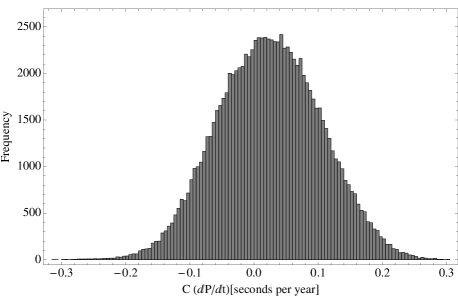
Figure 12.— Marginalized posterior distribution of the rate of change of the orbital period for TrES-2b ($C$). We find no evidence for a long-term change in the planet’s orbital period.

7.1.3 Hypothesis 3 - Systematic error in the Kepler times

The only contemporaneous transit measurement between Kepler and the professional measurements is insufficient to test this hypothesis. This is because the transit is question, measured by Mislis et al. (2010) for epoch 414, has a precision of 518 s and is therefore not useful for testing Kepler’s timing accuracy at the $<6.5$ s level.

In conclusion, the current body of evidence is insufficient to determine the cause of the discrepant periods. However, further transits from Kepler will resolve this issue in the future.

7.2. Duration Change

7.2.1 Comparing different bandpasses

As discussed in §6.5, Mislis & Schmitt (2009) claimed to have detected a linear decrease in the duration of TrES-2b due to the inclination angle varying at a rate of $0.195^{\circ}$ over $\sim$300 cycles, or $0.00065^{\circ}$ per cycle.

In order to look for evidence of long duration change, it is necessary to use data taken before the Kepler Mission. Holman et al. (2007) obtained three high-quality transits observations using the FLWO 1.2 m telescope, in anticipation of this requirement, with a mean cycle value of $20.\dot{6}$. In contrast, the Q0 and Q1 data have a mean cycle value of 412.5, giving a baseline to the FLWO data of $391.8\dot{3}$ cycles.

However, as also discussed in §6.5, we cannot compare data from different bandpasses unless we fit for limb darkening coefficients, especially since transit parameters are known to be acutely correlated to limb darkening for near-grazing transits (see §3.2.2 and §4.1). Holman et al. (2007) did not fit for limb darkening coefficients and so we here present a re-analysis of those three transits.

7.2.2 Re-analysis of Holman et al. (2007) photometry

We choose to fit for linear limb darkening due to the lower signal-to-noise from ground-based data. Using the corrected photometry from Holman et al. (2007), we perform these fits in the same manner used in this paper. We float $e\sin\omega$, $e\cos\omega$, $K$, $\gamma$ and $P$ around their best-fit values from the global eccentric run (see Table 2) to allow their errors to propagate into the MCMC. The results are reported in Table 4.

7.2.3 Choosing a statistic

In §6.1, we compared durations within the same bandpass and thus fixing limb darkening was justified. Since $\tilde{T}_{1}$ is highly correlated to the limb darkening coefficients, we find $T_{1,4}$ offers the highest signal-to-noise for TrES-2b when limb darkening is fitted and will be adopted here.

7.2.4 Limits on duration change

The Holman et al. (2007) global fit finds $T_{1,4}=6559_{-103}^{+102}$ s whereas the Kepler global fit finds $T_{1,4}=6439_{-28}^{+25}$ s, giving $\Delta T_{1,4}=(-120\pm 106)$ s over $391.8\dot{3}$ cycles, which we do not consider to be significant. The data exclude a decrease in the transit duration $|\Delta T_{1,4}|>438$ s, or 165 s per year, to 3-$\sigma$ confidence. In contrast, Mislis & Schmitt (2009) claim to have detected a duration decrease of $\sim 3.16$ minutes (189.6 s) over $\sim 300$ cycles (or 91 s per year). Whilst this is not supported by our analysis, it is also not excluded. Scuderi et al. (2010) have challenged the Mislis & Schmitt (2009) result recentlty using ground-based transit observations and the Gilliland et al. (2010) result. Future Kepler transits will resolve this issue definitively.

Table 4Results from re-analysis of TrES-2b using the Holman et al. (2007) photometry. Quoted values are medians of MCMC trials with errors given by 1-$\sigma$ quantiles. * = fixed parameter; $\dagger$ = parameter was floated but not fitted.

Parameter	Our fit	H07 value
$P$ [days]	$2.47061892_{-0.00000012}^{+0.00000018}$ $\dagger$	$2.470621\pm 0.000017$
$T_{1,4}$ [s]	$6559_{-103}^{+102}$	$6624\pm 72$
$\tilde{T}_{1}$ [s]	$4656_{-196}^{+155.6}$	-
$T_{2,3}$ [s]	$1706_{-913}^{+505}$	-
$(T_{1,2}\simeq T_{3,4})$ [s]	$2432_{-229}^{+411}$	$2459\pm 162$
$(R_{P}/R_{*})^{2}$ [%]	$1.674_{-0.118}^{+0.052}$	-
$b$	$0.848_{-0.018}^{+0.022}$	$0.8540\pm 0.0062$
$e\sin\omega$	$-0.009_{-0.029}^{+0.024}$ $\dagger$	$0^{*}$
$e\cos\omega$	$0.0005_{-0.0018}^{+0.0018}$ $\dagger$	$0^{*}$
$\Psi$	$0.973_{-0.082}^{+0.071}$ $\dagger$	$1^{*}$
$K$ [ms-1]	$181.0_{-5.4}^{+5.5}$ $\dagger$	-
$\gamma$ [ms-1]	$-29.2_{-2.6}^{+2.6}$ $\dagger$	-
$B$	$1.04246\pm 0.00023$ $\dagger$	$1^{*}$
$u_{1}$	$0.52_{-0.39}^{+0.18}$	$0.22^{*}$
$u_{2}$	$0^{\mathrm{*}}$	$0.32^{*}$
$R_{P}/R_{*}$	$0.1294_{-0.0046}^{+0.0020}$	$0.1253\pm 0.0010$
$a/R_{*}$	$7.93_{-0.24}^{+0.18}$	$7.63\pm 0.12$
$i$ [∘]	$83.99_{-0.35}^{+0.25}$	$83.57\pm 0.14$
$\rho_{*}$ [g cm-3]	$1543.4_{-135.6}^{+108.7}$	-
$\log(g_{P}\,[\mathrm{cgs}])$	$3.306_{-0.018}^{+0.018}$	-

8. SUMMARY OF RESULTS

Due to the large number of results presented in this paper, we summarize the key findings below:

• The Kepler SC data exhibit unprecedented precision with r.m.s. noise 237.2 ppm per 58.8 s.

• Fitting for limb darkening coefficients leads to much larger uncertainties in the system parameters of TrES-2b, due to the near-grazing nature of the orbit (e.g. a factor of 17.5 larger for the transit depth)

• We present a self-consistent, refined set of transit, radial velocity and physical parameters for the TrES-2b system, which are in close agreement with previous values.

• We do not detect an occultation of TrES-2b, constraining the depth to be $<72.9$ ppm to 3-$\sigma$ confidence, indicating that this object has the lowest measured geometric albedo for an exoplanet, of $A_{g}<0.146$.

• We detect no short or long term transit timing variations (TTV) in the TrES-2b system and exclude short-term signals of r.m.s. $>7.11$ s and a long-term variation of $0.11$ s per year in the orbital period, to 3-$\sigma$ confidence.

• We detect no short or long term transit duration variations (TDV) in the TrES-2b system and exclude short-term relative duration change of $>0.77$% and long-term change of $>2.5$% per year, to 3-$\sigma$ confidence.

• We exclude the presence of exomoons down to sub-Earth masses for TrES-2b.

• The Mislis & Schmitt (2009) hypothesis of long-term duration change is neither supported nor refuted by our analysis.

• We find the Rabus et al. (2009) hypothesis of a 0.2 cycle TTV is not supported by the Kepler photometry, to a high confidence level.

• We find no evidence for other dips in the lightcurve as reported by Raetz et al. (2009).

Table 5All measured transit times of TrES-2b taken from the literature, the ETD (Exoplanet Trasnit Database) and this work, at the time of writing. * = value presented in Mislis & Schmitt (2009) and Mislis et al. (2010) for this transit do not agree with each other and therefore these measurements are not included in our long-term TTV analysis. $\dagger$ = value comes from summing more than one transit lightcurve. ** = times are in BJD_TDB.

Epoch	$\tau$ [HJDUTC-2,450,000]	Reference	Epoch	$\tau$ [HJDUTC-2,450,000]	Reference
000	$3957.63580\pm 0.00100$	O’Donovan et al. (2007)	391	$4923.64380\pm 0.00070$	ETD
004	$3967.51800\pm 0.00043$	Rabus et al. (2009)	393	$4928.58752\pm 0.00143$	ETD
012	$3987.28000\pm 0.00800$	ETD	393	$4928.58757\pm 0.00626$	ETD
013	$3989.75286\pm 0.00029$	Holman et al. (2007)	393	$4928.58792\pm 0.00112$	ETD
015	$3994.69393\pm 0.00031$	Holman et al. (2007)	395	$4933.52740\pm 0.00076$	Mislis et al. (2010)
019	$4004.57500\pm 0.00140$	ETD	395	$4933.52726\pm 0.00168$	ETD
025	$4019.40150\pm 0.00600$	ETD	399	$4943.41320\pm 0.00138$	ETD
034	$4041.63579\pm 0.00030$	Holman et al. (2007)	404	$4955.763285_{-0.000055}^{+0.000055}$	This work **
087	$4172.57670\pm 0.00160$	Raetz et al. (2009)	405	$4958.233958_{-0.000056}^{+0.000056}$	This work **
106	$4219.52050\pm 0.00600$	ETD	406	$4960.704556_{-0.000054}^{+0.000054}$	This work **
108	$4224.46176\pm 0.00250$	Raetz et al. (2009)	407	$4963.175188_{-0.000056}^{+0.000056}$	This work **
127	$4271.39911\pm 0.00297$	ETD	408	$4965.645708_{-0.000054}^{+0.000054}$	This work **
130	$4278.81790\pm 0.00600$	ETD	409	$4968.116367_{-0.000053}^{+0.000053}$	This work **
138	$4298.57880\pm 0.00240$	Raetz et al. (2009)	410	$4970.587001_{-0.000056}^{+0.000056}$	This work **
140	$4303.52090\pm 0.00030$	Rabus et al. (2009)	410	$4970.58650\pm 0.00100$	ETD
142	$4308.46130\pm 0.00045$	Rabus et al. (2009)	411	$4973.057600_{-0.000057}^{+0.000056}$	This work **
142	$4308.46448\pm 0.00130$	Raetz et al. (2009)	412	$4975.528262_{-0.000058}^{+0.000059}$	This work **
142	$4308.46240\pm 0.00600$	ETD	412	$4975.52630\pm 0.00150$	ETD
142	$4308.46300\pm 0.00180$	ETD	412	$4975.52790\pm 0.00090$	ETD
151	$4330.70130\pm 0.00200$	ETD	413	$4977.998830_{-0.000057}^{+0.000057}$	This work **
155	$4340.58350\pm 0.00120$	ETD	414	$4980.469389_{-0.000056}^{+0.000056}$	This work **
157	$4345.51390\pm 0.00160$	ETD	414	$4980.46750\pm 0.00060$	Mislis et al. (2010) $\dagger$
157	$4345.51990\pm 0.00120$	ETD	414	$4980.46450\pm 0.00130$	ETD
157	$4345.52350\pm 0.00150$	ETD	414	$4980.46790\pm 0.00170$	ETD
163	$4360.34550\pm 0.00109$	Raetz et al. (2009) $\dagger$	414	$4980.46820\pm 0.00130$	ETD
165	$4365.28746\pm 0.00210$	Raetz et al. (2009)	415	$4982.939972_{-0.000058}^{+0.000058}$	This work **
170	$4377.63810\pm 0.00070$	ETD	416	$4985.410672_{-0.000055}^{+0.000055}$	This work **
170	$4377.64230\pm 0.00120$	ETD	417	$4987.881247_{-0.000055}^{+0.000055}$	This work **
174	$4387.52220\pm 0.00150$	Raetz et al. (2009)	418	$4990.351850_{-0.000056}^{+0.000056}$	This work **
229	$4523.40970\pm 0.00080$	ETD	419	$4992.822571_{-0.000055}^{+0.000056}$	This work **
242	$4555.52621\pm 0.00123$	ETD	420	$4995.293071_{-0.000057}^{+0.000056}$	This work **
242	$4555.52360\pm 0.00090$	ETD	421	$4997.763671_{-0.000058}^{+0.000059}$	This work **
259	$4597.52250\pm 0.00120$	ETD	421	$4997.76286\pm 0.00035$	ETD
263	$4607.40360\pm 0.00720$	Mislis & Schmitt (2009)	423	$5002.70200\pm 0.00090$	ETD
268	$4619.75990\pm 0.00130$	ETD	425	$5007.64270\pm 0.00190$	ETD
272	$4629.64510\pm 0.00240$	ETD	429	$5017.52520\pm 0.00100$	ETD
274	$4634.58280\pm 0.00030$	Rabus et al. (2009)	433	$5027.40740\pm 0.00190$	ETD
276	$4639.52320\pm 0.00031$	Rabus et al. (2009)	438	$5039.76060\pm 0.00110$	ETD
278	$4644.46608\pm 0.00140$	Raetz et al. (2009)	438	$5039.76480\pm 0.00070$	ETD
278	$4644.46440\pm 0.00180$	ETD	438	$5039.76607\pm 0.00096$	ETD
280	$4649.41490\pm 0.00330$	ETD	438	$5039.76680\pm 0.00120$	ETD
281	$4651.87560\pm 0.00070$	ETD	440	$5044.70310\pm 0.00080$	ETD
293	$4681.52240\pm 0.00210$	ETD	442	$5049.64530\pm 0.00120$	ETD
304	$4708.69870\pm 0.00110$	ETD	442	$5049.64940\pm 0.00085$	ETD
310	$4723.51790\pm 0.00190$	ETD	446	$5059.52244\pm 0.00076$	ETD
312	$4728.47400\pm 0.00710$	Mislis & Schmitt (2009) *	548	$5311.53095\pm 0.00077$	ETD
312	$4728.46400\pm 0.00710$	Mislis et al. (2010) *	550	$5316.47653\pm 0.00094$	ETD
316	$4738.35215\pm 0.00200$	Raetz et al. (2009)	552	$5321.41833\pm 0.00137$	ETD
316	$4738.35045\pm 0.00090$	ETD	555	$5328.82558\pm 0.00093$	ETD
318	$4743.28972\pm 0.00180$	Raetz et al. (2009)	557	$5333.76390\pm 0.00107$	ETD
321	$4750.70010\pm 0.00110$	ETD	557	$5333.76469\pm 0.00123$	ETD
333	$4780.34690\pm 0.00220$	ETD	567	$5358.47237\pm 0.00071$	ETD

References

- Agol et al. (2005) Agol, E., Steffen, J., Sari, R. & Clarkson, W. 2005, MNRAS, 359, 567
- Ahmed et al. (1974) Ahmed, N., T. Natarajan, T., & K. R. Rao, K. R. 1974, IEEE Trans. Computers, 90
- Allan (1966) Allan, D. 1966, Proceedings of IEEE, 54, 221-230
- Bakos et al. (2009) Bakos, G. A. et al. 2009, ApJ, 710, 1724
- Basri et al. (2005) Basri, G., Borucki, W. J. & Koch, D., 2005, New Astronomy Rev., 49, 478
- Carter et al. (2008) Carter, J. A., Yee, J. C., Eastman, J., Gaudi, B. S. & Winn, J. N., 2008, ApJ, 689, 499
- Carter et al. (2009) Carter, J. A., Winn, J. N., Gilliland, R. & Holman, M. J. 2009, ApJ, 696, 241
- Carter et al. (2010) Carter, J. A.& Winn, J. N., 2009, ApJ, 704, 51
- Carter & Winn (2010) Carter, J. A. & Winn, J. N., 2010, ApJ, 716, 850
- Claret (2000) Claret A., 2000, A&A, 363, 1081
- Czesla et al. (2009) Czesla, S., Huber, K. F., Wolter, U., Schroter, S. & Schmitt, J. H. M. M. 2009, A&A, 505, 1277
- Daemgen et al. (2009) Daemgen, S., Hormuth, F., Brandner, W., Bergfors, C., Janson, M., Hippler, S. & Henning, T., 2009, A&A, 498, 567
- Díaz-Cordovés et al. (1995) Díaz-Cordovés, J., Claret, A., & Giménez, A., 1995, A&AS, 110, 329
- Domingos et al. (2006) Domingos, R. C., Winter, O. C. & Yokoyama, T., 2006, MNRAS, 373, 1227
- O’Donovan et al. (2007) O’Donovan, F. T. et al., 2007, ApJ, 651, 61
- O’Donovan et al. (2010) O’Donovan, F. T., Charbonneau, D., Harrington, J., Madhusudhan, N., Seager, S., Deming, D., Knutson, H. A., 2010, ApJ, 710, 1551
- Eastman et al. (2010) Eastman, J., Siverd, R., Gaudi, B. S., 2010, PASP, submitted
- Gilliland et al. (2010) Gilliland, R. L. et al., 2010, ApJL, 713, 160
- Ford (2005) Ford, E. B. 2005, AJ, 129, 1706
- Ford & Gaudi (2006) Ford, E. B. & Gaudi, S. B. 2006, ApJ, 652, 137
- Ford & Holman (2007) Ford, E. B. & Holman, M. J., 2007, ApJ, 664, 51
- Holman & Murray (2005) Holman, M. J. & Murray, N. W., 2005, Science, 307, 1288
- Holman et al. (2006) Holman, M. J. et al., 2006, ApJ, 652, 1715
- Holman et al. (2007) Holman, M. J. et al., 2007, ApJ, 664, 1185
- Holman et al. (2010) Holman, M. J. et al., 2007, Science, 330, 51
- Kipping (2008) Kipping, D. M., 2008, MNRAS, 389, 1383
- Kipping (2009a) Kipping, D. M., 2009a, MNRAS, 392, 181
- Kipping (2009b) Kipping, D. M., 2009b, MNRAS, 396, 1797
- Kipping (2009) Kipping, D. M., Fossey, S. J. & Campanella, G., 2009, MNRAS, 400, 398
- Kipping (2010a) Kipping, D. M., 2010a, MNRAS, 407, 301
- Kipping & Bakos (2010) Kipping, D. M. & Bakos, G. A., 2010, ApJ, accepted
- Kipping & Tinetti (2010) Kipping, D. M. & Tinetti, G., 2010, MNRAS, 407, 2589
- Kipping et al. (2011) Kipping, D. M. et al., 2010, ApJ, 725, 2017
- Koch et al. (2007) Koch, D., Borucki, W., Basri, G. et al., 2007, in W.I. Hartkopf, E.F. Guinan & P. Harmanec (eds.), ‘Binary Stars as Critical Tools & Tests in Contemporary Astrophysics’, Proc. IAU Symp. 240, p.236 (Cambridge University Press, Cambridge)
- Kurucz (2006) Kurucz R., 2006, Stellar Model and Associated Spectra (http://kurucz.harvard.edu/grids.html)
- Liddle et al. (2007) Liddle, A. R. 2007, MNRAS, 377, L74
- Mandel & Agol (2002) Mandel, K. & Agol, E., 2002, ApJ, 580, 171
- Mazeh et al. (2010) Mazeh, T. & Faigler, S., 2010, A&A, 521, 59
- Miralda-Escudé (2002) Miralda-Escudé, J., 2002, ApJ, 564, 1019
- Mislis & Schmitt (2009) Mislis, D. & Schmitt, J. H. M. M., 2009, A&A, 500, 45
- Mislis et al. (2010) Mislis, D., Schroter, S., Schmitt, J. H. M. M., Cordes, O. & Reif, K., 2010, A&A, 510, 107
- Pál (2008) Pál, A., 2008, MNRAS, 390, 281
- Raetz et al. (2009) Raetz, St. et al., 2009, ASNA, 330, 459
- Rabus et al. (2009) Rabus, M., Deeg, H. J., Alonso, R., Belmonte, J. A. & Almenara, J. M., 2009, A&A, 508, 1011
- Rowe et al. (2008) Rowe, J. F. et al., 2008, ApJ, 689, 1345
- Sartoretti & Schneider (1999) Sartoretti, P. & Schneider, J., 1999, A&AS, 14, 550
- Schwarz (1978) Schwarz, G. 1978, The Annals of Statistics, 6, 461
- Scuderi et al. (2010) Scuderi, L. J., Dittmann, J. A., Males, J. R., Green, E. M. & Close, L. M., 2010, ApJ, 714, 462
- Seager & Mallén-Ornelas (2003) Seager, S., & Mallén-Ornelas, G., 2003, ApJ, 585, 1038
- Spiegel & Burrows (2010) Spiegel, D. S. & Burrows, A., 2010, ApJ, submitted
- Sozzetti et al. (2007) Sozzetti, A., Torres, G., Charbonneau, D., Latham, D. W., Holman, M. J., Winn, J. N., Laird, J. B. & O’Donovan, F. T., ApJ, 664, 1190
- Tegmark et al. (2004) Tegmark, M., 2004, Phys. Rev. D, 69, 103501
- Winn et al. (2008) Winn, J. et al., 2008, ApJ, 682, 1283
- Yi et al. (2001) Yi, S. K. et al. 2001, ApJS, 136, 417