Ideal magnetohydrodynamic simulations of unmagnetized dense plasma jet injection into a hot strongly magnetized plasma

Abstract

We present results from three-dimensional ideal magnetohydrodynamic simulations of unmagnetized dense plasma jet injection into a uniform hot strongly magnetized plasma, with the aim of providing insight into core fueling of a tokamak with parameters relevant for ITER and NSTX (National Spherical Torus Experiment). Unmagnetized dense plasma jet injection is similar to compact toroid injection but with much higher plasma density and total mass, and consequently lower required injection velocity. Mass deposition of the jet into the background appears to be facilitated via magnetic reconnection along the jet’s trailing edge. The penetration depth of the plasma jet into the background plasma is mostly dependent on the jet’s initial kinetic energy, and a key requirement for spatially localized mass deposition is for the jet’s slowing-down time to be less than the time for the perturbed background magnetic flux to relax due to magnetic reconnection. This work suggests that more accurate treatment of reconnection is needed to fully model this problem. Parameters for unmagnetized dense plasma jet injection are identified for localized core deposition as well as edge localized mode (ELM) pacing applications in ITER and NSTX-relevant regimes.

1 Introduction

It is important to deliver fuel into the core of a tokamak fusion plasma to maintain steady-state operation, achieve more efficient utilization of the deuterium-tritium fuel, and optimize the energy confinement time [1]. The subject of plasma fueling and density profile control is important for the successful operation of a future reactor-grade tokamak such as ITER [2]. The injected fuel must have sufficiently high directed energy to penetrate the strongly magnetized edge plasma and reach the core [3, 4]. A total particle inventory of $10^{18}$–$10^{23}$ and a flow velocity of up to 800 km/s (depending on injected density) are required [5]. It is desirable for plasmas to be deposited not only deeply but also precisely in order to optimize bootstrap current and maintain optimized fusion burn conditions [5, 6]. Several fueling schemes have been proposed, such as gas injection, pellet injection [7], neutral beam injection, and compact toroid (CT) injection [8]. All these methods will have difficulties achieving localized core deposition in a reactor grade tokamak plasma [5].

Injection of unmagnetized (or weakly magnetized) dense plasma jets is an alternative to the above methods. This is most similar to CT injection in concept, but with the key advantages of having much higher density (which allows lower injection velocities) and injector hardware with a smaller footprint than CT injector/accelerators (allowing for versatile placement of many injector units around the tokamak). Unmagnetized dense plasma jets produced by a two-stage pulsed plasma source [9] were successfully injected deeply into the spherical tokamak Globus-M [3, 5]. In addition, very recent developments in coaxial gun and mini-railgun technology utilizing a pre-ionized fill plasma [10] (of any gas species) make it timely to use modern simulation tools to gain insight into the penetration and injection dynamics of unmagnetized dense plasma jets into an ITER or NSTX-like (National Spherical Torus Experiment) [11] plasma. Unmagnetized dense plasma jet injection may also potentially find applications for edge localized mode (ELM) pacing [12] and disruption mitigation [13].

Recent simulation results [4] indicate that low $\beta$ CT injection has the potential to deposit fuel in a precise manner at any point in the machine, from the edge to the core, although a very high injection speed is required. Since a CT plasma is confined by its magnetic field, its density is limited. The plasma volume needs to be increased to accommodate a larger total number of particles [3, 5]. Preliminary simulation results [4] of unmagnetized dense plasma jets injected into an ITER-relevant background plasma suggest that deep but somewhat less-localized fueling (compared to CT’s) is possible for unmagnetized dense plasma jet injection. In this paper, we employ a simple idealized model and three-dimensional (3D) ideal magnetohydrodynamic (MHD) simulations of unmagnetized dense plasma jets propagating into a uniform slab plasma with uniform magnetic field perpendicular to the jet propagation direction, mimicking jet fueling into an infinite aspect ratio tokamak. As we point out throughout this paper, an ideal MHD treatment cannot capture all of the important dynamics of this problem accurately. Our aim in this work is to provide initial insight into the essential physics occurring during unmagnetized dense plasma jet injection, and point the way toward progressively more sophisticated physics models and simulation tools that will be required, e.g., resistive MHD and two-fluid models, as well as the inclusion of realistic tokamak profiles and geometry (including finite aspect ratio). Most of the present results focus on ITER-relevant parameters and injection velocities (Table 1). In addition, some preliminary results are discussed for NSTX-relevant parameters (Table 2).

For completeness, we briefly place this work into the context of a substantial body of research that has focused on CT injection for tokamak refueling. The conducting sphere (CS) theoretical model was put forth some twenty years ago [8, 1, 14] and described the injection of a rigid conducting ball into a strongly magnetized background plasma. In the CS model, the Alfvén speed of the background plasma is much higher than the speed of the injected CT, and thus the background field can rearrange itself virtually instantaneously in response to the injected CT. In the CS model, it is the magnetic field pressure gradient of the background plasma that eventually brings the injected CT to a stop. More precisely, the injected CT stops when the background magnetic energy excluded by the CT volume approximately equals the CT’s initial kinetic energy. Later, Suzuki et al. [15, 16, 17] performed MHD numerical simulations taking into account the compressibility of the injected plasma. They found, by carefully analyzing the energetics of the evolution of the injected CT, that the effects of plasma compressibility are critical for slowing down the injected plasma. Plasma compressibility leads to the modification of both the magnetic field and density at the leading and side interfaces between the injected and background plasmas. Therefore the speed of localized Alfvénic and acoustic dynamics of this interfacial region becomes of the same order as the injection speed, and thus the perturbed background field and density no longer can respond instantaneously to the injected plasma. This, in combination with the higher injection velocities treated in our work, leads to the situation where the background field can be “stretched” by the injected plasma, as shown both in Suzuki et al.’s and our simulation results, with field line tension thus playing a significant role in stopping the injected plasma. We note that our recent work [4] and the present work extend the work of Suzuki et al. by treating higher ratios of background-to-injected magnetic field strength ($>10$) and density (up to 1000), respectively, for the problem of plasma injection into tokamaks. Finally, within the context of supersonic gas injection, the effects of jet heating (by the hot background tokamak plasma) and polarization electric field (within the jet) on jet penetration have been considered [18]. Accurate modeling of these effects is beyond the capabilities of our compressible MHD code, and thus future work using a two-fluid code with a better heating model is needed to definitively evaluate these effects.

The paper is organized as follows. Section 2 describes the computational model and problem setup. In Sec. 3, simulation results on unmagnetized dense plasma jet injection and evolution are presented for an ITER-relevant scenario (Table 1). Conclusions and also implications for ELM pacing, disruption mitigation, and NSTX-relevant (Table 2) jet injection are given in Sec. 4.

2 Computational model

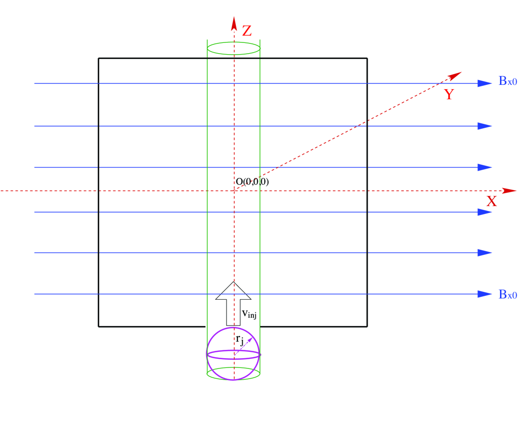
Figure 1:  (Color online) Schematic of the simulation geometry showing the coordinate system, the background magnetic field, the injected plasma (with spherical radius $r_{j}=0.5$), and the background plasma (cubic with sides of length $=18$).

An unmagnetized and high density ($\sim 10^{17}\,{\rm cm^{-3}}$) plasma jet with spherical radius $r_{j}=0.5$, centered initially at $X=0$, $Y=0$ and $Z=Z_{0}=-10$, is injected along the $Z$ axis into a lower density background plasma with injection velocity $v_{\rm inj}$ (see Fig. 1). The background plasma is a cube with sides of length $=18$. We use the term “jet” because eventually higher injected mass will require that the ball become elongated into a cylindrical “jet.” The model equations, assumptions, and numerical treatments are essentially the same as those in a recent paper on CT injection [4], except that the jet has spatially uniform density rather than the double-peaked profile of a CT. The background plasma has a uniform magnetic field (no gradient). However, for the regimes considered in this paper, stopping of the injected plasma is provided mostly by field line tension of the distorted background plasma, and thus our results are expected to only slightly over-estimate the penetration depth. Our 3D ideal MHD code uses high-order Godunov-type finite-volume numerical methods. These methods conservatively update the zone-averaged fluid and magnetic field quantities based on estimated advective fluxes of mass, momentum, energy, and magnetic field at the zone interface [19]. The divergence-free condition of the magnetic field is ensured by a constrained transport scheme [20]. All simulations were performed on parallel Linux clusters at Los Alamos National Laboratory. We note that the details of magnetic reconnection and heat evolution are not captured accurately due to the ideal MHD model and the use of a simplified energy equation, and that future work using more sophisticated models are needed to refine any reconnection-dependent conclusions given in this work.

Physical quantities are normalized by the characteristic system length scale $R_{0}=10\;\,{\rm cm}$, mass density $\rho_{0}=7.77\times 10^{-9}\;\,{\rm g/cm^{-3}}$ (corresponding to a 50%-50% DT mixture ion number density $n_{0}=1.86\times 10^{15}\;\,{\rm cm^{-3}}$), and velocity $V_{0}=1.7\times 10^{8}\;\,{\rm cm\;s^{-1}}$. Other quantities are normalized as (for the ITER-relevant case of Table 1): time $t=1$ gives $R_{0}/V_{0}=59\,{\rm ns}$, magnetic field $B=1$ gives $(4\pi\rho_{0}V_{0}^{2})^{1/2}=5.3\times 10^{4}\;\,{\rm G}$, and energy $E=1$ gives $\rho_{0}V_{0}^{2}R_{0}^{3}=2.24\times 10^{11}\;\,{\rm ergs}$. The boundary conditions are all perfectly conducting in the $Y$ and $Z$ directions except at the entrance port of the bottom boundary (analogous to the tokamak edge) where the jet is injected, while in the $X$ direction non-reflecting outflow boundary conditions [21] are employed in order to mimic the toroidal geometry of a tokamak. The outflowing boundary condition is stress-free, and thus the magnetic flux is not “line-tied” to the walls and Alfvén dynamics are supported along $X$ despite the small simulation domain. Suzuki et al. [17] have performed simulations with toroidal periodic boundary conditions. They found that with such a stress-free boundary condition, the magnetic tension force is smaller (but not zero), and the relaxation of the tension force from magnetic reconnection is also much smaller (could even be ignored). An outflowing boundary condition is more appropriate than Suzuki et al.’s choice for the large aspect ratio case since in real tokamaks the toroidal dimension is much larger than the poloidal dimension, and thus it will take a long time for toroidal dynamics to re-enter the computational domain after traveling along toroidal magnetic field lines [4]. In order to minimize the influence of the entrance port on boundary conditions, the port is opened (a hole inserted into the conducting boundary) when the top of the jet reaches the bottom boundary at $t=0.5/v_{\rm inj}$ and is closed (hole removed from the conducting boundary) at $t=2/v_{\rm inj}$ after the jet has fully entered the computation domain (at $t\sim 1.5/v_{\rm inj}$). This leads to an artificial force pulling back on the injected plasma which is apparent only at late times for simulations with shallow injection (as shown in Fig. 7) and does not otherwise appear to significantly affect the injected plasma evolution.

In order to mimic jet injection into an ITER-relevant plasma, we adopt physical quantities as given in Table 1 in most of the results reported in this paper. The major differences here compared to the recent results on CT injection [4] are the very high density ratio $n_{j}/n_{p}\gtrsim 500$ (where $n_{j}$ and $n_{p}$ are the injected and background plasma densities, respectively) and the initially null value of the jet magnetic field. The computational domain coinciding with the background plasma is $|X|\leq 9$, $|Y|\leq 9$, and $|Z|\leq 9$, corresponding to a cube of $(180\;\,{\rm cm})^{3}$ in actual length units (assuming the injected jet radius $r_{j}=5\;\,{\rm cm}$). The numerical resolution used here is $400\times 400\times 800$, where the grid points are assigned uniformly in the $X$, $Y$, and $Z$ directions. A cell $\delta X$ $(=\delta Y=2\delta Z=0.045$) corresponds to $0.45\;\,{\rm cm}$. Since the plasma skin depth and ion gyroradius based on either ITER or NSTX parameters are no more than $\delta X$, simulations based on an MHD model are reasonable for this initial study.

3 Results

3.1 Injected plasma jet evolution

Figure 2 displays the evolution of magnetic field $B_{xz}$ (arrows) and current density $j_{y}$ (color contours) in the $X$-$Z$ plane at $Y=0$ with parameters given in Table 1. During the initial jet penetration into the background plasma, the jet meets a very strong magnetic barrier. Thus, the plasma jet becomes compressed along the direction of propagation ($Z$) by about 30% at $t=20$ but not much in $X$ (by examining the $\rho$ profile versus $Z$ and $X$ at $t=15$ and 20, not shown here), and the background magnetic field gets distorted as seen in Fig. 2(a). The plasma density increases at the jet-background interface. A large plasma current also appears there due to the compression of the background magnetic field, as seen in Fig. 2(a) and the edges of the jet (return current). Magnetic fields diffuse into the jet due to numerical resistivity with resistive diffusion time $\tau_{res}\sim 10.9$ [4]. For a real jet injected into a real tokamak, the magnetic diffusion time into the jet will likely be somewhat slower, and more sophisticated simulations (e.g., using a resistive MHD or two-fluid code) and ultimately experiments will be needed to fully assess this. However, we believe that the field diffusion into the jet is not critically important for the further dynamics to be described below. The magnetic tension force due to the stretched field lines persists even with our stress-free boundary conditions (i.e., it is not a result of line-tying), although it is smaller than with fixed boundary conditions [17]. From Figs. 2(a) and (b), the speed at which the background field distortion propagates away along the $X$ direction can be crudely estimated as $\Delta X/\Delta t\sim 0.5/10\sim 0.05$, which is slower than $v_{\rm inj}=0.12$. In addition, Fig. 3 shows the local values of the Alfvén ($V_{A}$) and ion acoustic ($C_{s}$) speeds versus $Z$ at $t=15$ and $t=20$. For example, at $t=20$, the jet/background interfacial region is centered near $Z=-7.4$ as seen from Fig. 2(b), at which location both $V_{A}$ and $C_{s}$ are of the order 0.05 as seen in Fig. 3. Thus, neither Alfvén nor acoustic waves are fast enough to instantaneously relax the perturbations in magnetic field and density at the jet/background interface. Finally, tilting of the plasma jet is not observed due to the fast injection and short jet transit time.

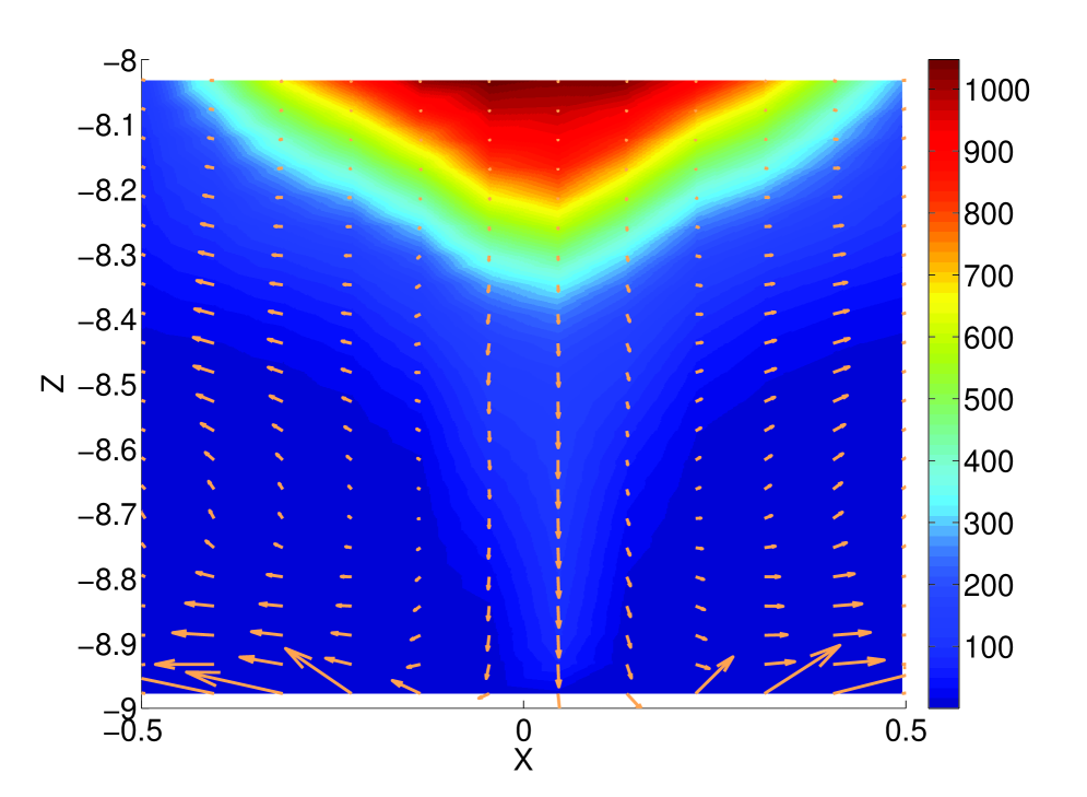
Figure 4:  (Color online) Contours of $\rho$ and vectors of $\vec{v}=(v_{x},v_{z})$ (in jet frame of reference) at $t=20$ ($1.18\,{\rm\mu s}$) for parameters of Table 1.

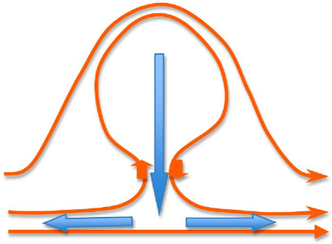
Figure 5:  (Color online) Schematic of the magnetic configuration around $t=20$. Solid orange lines indicate magnetic field lines, while solid blue arrows indicate internal jet plasma flows (in jet frame of reference). Opposing orange arrows indicate anti-parallel magnetic field where reconnection occurs.

After the jet has fully entered the background plasma region (after $t\sim 20$), a region with magnetic field reversal is set up along the jet’s trailing edge, centered about $X=0$ and $Z\approx-8.4$ in Fig. 2(b). This enables magnetic reconnection [22] which as pointed out by Suzuki et al. [16] allows the jet to be “detached” from the background field lines and by which the magnetic tension force decelerating the jet is relaxed. Clearly, any reconnection observed in our results is due to numerical resistivity (see further discussion in Sec. 3.2). Figure 4 shows velocity vectors, from which [along with Fig. 2(b)] we infer a jet configuration at $t=20$ shown schematically in Fig. 5. The primary reconnection site is located at the trailing portion of the jet along $Z$. This is qualitatively different from CT fueling in which reconnection takes place at the upper left and lower right areas of the CT (due to the asymmetric CT field) [4]. The reconnection process allows the plasma within the jet to escape and eventually flow outward along the background magnetic field horizontally (toroidally), as shown in Figs. 4 and 5. Thus reconnection facilitates mass deposition from the jet into the background plasma. We note that mass deposition into the tokamak plasma was indeed observed for unmagnetized plasma injection on Globus-M [3, 5] although neutralization of their jet in transit could also lead to mass deposition without requiring reconnection. The latter needs further study including atomic physics modeling. The initial $Z$-directed kinetic energy is converted into $X$-directed kinetic energy. After the high density jet plasma has been depleted (after $t\sim 50$), the perturbed background field has nearly oriented again along $X$, the direction of the initial background magnetic field [Fig. 2(d)].

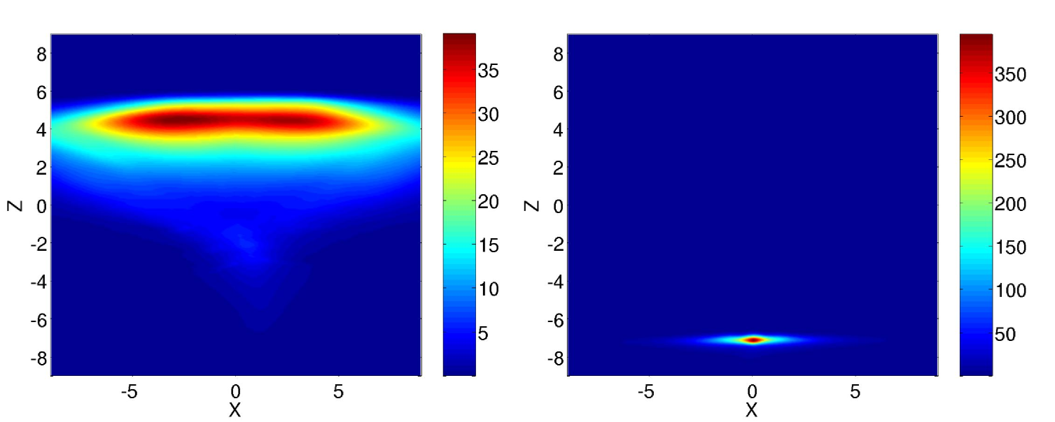
Figure 6:  (Color online) (left) Density contours at $Y=0$ and $t=150$ for parameters of Table 1, showing deep but not highly localized deposition. The jet is still moving at nearly the initial injection speed. (right) Density contours at $Y=0$ and $t=80$ with the same parameters except $v_{\rm inj}=0.056$ ($93.3\,{\rm km/s}$), showing shallow but more localized deposition. Note that the color scales are not identical.

Figure 6(left) shows contours of density in the $X$-$Z$ plane ($Y=0$) at $t=150$ for the parameters of Table 1, showing deep jet penetration. From Fig. 6(left), the spread $\Delta Z\sim 3.5$ ($35\,{\rm cm}$) of this line-shaped structure is much larger than for CT fueling [4] which is about $\Delta Z\sim 0.2$ ($2\,{\rm cm}$). The jet in Fig. 6(left) does not come to rest fully, but a jet with lower injection velocity should come to rest deep in the background plasma. Note that, by comparing with Fig. 2(d), the perturbed background magnetic flux has mostly relaxed by $t=50$ while the diminishing jet mass has reached $Z\approx 4$ as shown in Fig. 6(left). However, under proper conditions (see further discussion in Sec. 3.2), the jet mass can be deposited more locally around the jet stopping position, as seen in Fig. 6(right) with lower $v_{\rm inj}=0.056$. A narrow elongated structure along $X$ with penetration depth $2.7$ ($27\,{\rm cm}$) and a spread of $\Delta Z\sim 0.5$ ($5\,{\rm cm}$) results. In order to improve the precision of deposition, either lower injection speed, lower initial jet mass, or larger background magnetic field is necessary (see further discussion in Sec. 3.2).

3.2 Penetration depth and localized deposition

The penetration depth is mostly determined by the initial jet kinetic energy. With the magnetic tension force from the background magnetic field $F_{\rm tension}\propto B_{p}$, the deceleration of the jet is $a_{\rm jet}=F_{\rm tension}/M_{\rm jet}$, where $M_{\rm jet}$ is the jet initial mass. Note that Suzuki et al. [17] showed that the CT penetration depth, based on a model with magnetic tension force as the main deceleration mechanism, matches simulation results very well, implying that MHD wave drag forces may not be important in CT deceleration. If the jet is undergoing a constant deceleration (a rough estimate), the time for the jet to stop is: $T_{\rm slowdown}=v_{\rm inj}/a_{\rm jet}=v_{\rm inj}M_{\rm jet}/F_{\rm tension}$. Thus the penetration depth $S$ of the jet would be:

$$S=\frac{1}{2}v_{\rm inj}T_{\rm slowdown}=\frac{1}{2}M_{\rm jet}v_{\rm inj}^{2}/F_{\rm tension}=E_{K0}/F_{\rm tension}\;,$$ (1)

where $E_{K0}=M_{\rm jet}v_{\rm inj}^{2}/2$ is the jet’s initial kinetic energy. Based on this estimate, the penetration depth is roughly proportional to the jet initial kinetic energy and inversely proportional to the magnetic tension force, which is proportional to the background magnetic field. The CS model [1] shows that a CT would penetrate to a position where the initial CT kinetic energy exceeds the background magnetic field energy excluded by the CT volume, and a lower limit of injection speed $V_{\rm AC}$ was derived from this requirement [4]. However, our simulation results [Fig. 6(left)] with $v_{\rm inj}=0.12<V_{\rm AC}=0.136$ (for Table 1 parameters) show that the jet penetrates the background field easily, which was also observed experimentally [5, 3]. Instead, the jet must have sufficiently high directed energy to overcome the deceleration from the magnetic tension force. Of course, as mentioned previously, another possibility is that a sizable fraction of the initial jet plasma is transformed into neutrals, which results in more efficient penetration of particles into a magnetic field [3]. A more detailed study including the effects of atomic physics (especially three body recombination) is needed to fully assess the role of jet neutralization during transit.

For internal density profile control, plasmas need to be deposited not only deeply but also precisely [5, 6]. Based on the mechanism of jet mass deposition put forth in Sec. 3.1, a key requirement for localized deposition is therefore to have the jet slowing-down time be less than the time for the perturbed magnetic flux to relax due to magnetic reconnection, $v_{\rm inj}M_{\rm jet}/F_{\rm tension}\lesssim\tau_{\rm res}$. Therefore lower injection speed (but exceeding the threshold for penetration), smaller initial mass, and larger background magnetic field are favorable for accurate deposition but unfavorable for depositing high mass into the core of the tokamak. Figure 6(right) with $v_{\rm inj}=0.056$ ($93\,{\rm km\;s^{-1}}$) and initial jet mass $0.22\,{\rm mg}$ shows a relatively shallow but local deposition case with penetration depth $S=2.7$ ($27\,{\rm cm}$) and spread $\Delta Z\sim 0.5$ ($5\,{\rm cm}$); this shallow deposition scenario may be useful for ELM pacing applications (see discussion in Sec. 4). Jet fueling might increase the background plasma inventory by $\sim 50\%$ in a single shot without disturbing background plasmas parameters [Fig. 6(right)]. Voronin et al. [3] reported an unmagnetized dense plasma jet source with an injection speed $\sim 110\,{\rm km\;s^{-1}}$. Coaxial guns and mini-railguns under development by HyperV Technologies Corp. [10] have achieved peak jet velocities of $100\,{\rm km\;s^{-1}}$, total masses up to $4\,{\rm mg}$, and peak particle densities up to a few times $10^{17}\,{\rm cm^{-3}}$, although all the peak values have not yet been achieved simultaneously. An unmagnetized dense plasma jet with injection speed between $0.056$ ($93\,{\rm km\;s^{-1}}$) and $0.12$ ($200\,{\rm km\;s^{-1}}$) with particle number density $10^{17}$ cm^-3 is achievable experimentally in the near term and might give deeper and localized deposition.

Finally, due to the potentially important role played by the reconnection time of the perturbed magnetic flux for localized deposition, we evaluate how the effective Lundquist number arising from numerical resistivity in our ideal MHD simulation compares with the Lundquist number for the situation in a real tokamak. At $t=40$, the Alfvén speed $V_{A}$ and the thickness $L_{\rm sheet}$ of the current sheet at the leading edge of the jet are found to be $7.5$ and $0.3$ from the simulation, respectively, corresponding to an effective Lundquist number $=\tau_{\rm res}V_{A}/L_{\rm sheet}=250$ due to numerical resistivity. For the real situation, we assume Spitzer conductivity, $\sigma=1.9\times 10^{4}T_{e}^{3/2}Z\ln\Lambda\;\,{\rm(Ohm\;m)^{-1}}$, where the electron temperature $T_{e}$ is in $\,{\rm eV}$ and the Coulomb logarithm is $\ln\Lambda=\ln(12\pi\epsilon_{0}^{3/2}T_{e}^{3/2}/Ze^{2/3}n_{e}^{1/2})$. The magnetic diffusivity is $\eta=1/\mu_{0}\sigma$. Given $n_{e}=1\times 10^{17}\,{\rm cm^{-3}}$ and $T_{e}=2.5\,{\rm eV}$ as in Table 1, we get $\eta=51\times 10^{4}\,{\rm cm^{2}\;s^{-1}}$, which gives a Lundquist number $=V_{A}L_{\rm sheet}/\eta=7500$ for the real situation. Thus, the effective Lundquist number for jet-background interactions in our simulations is much smaller than the likely real value in a tokamak, meaning that our simulation results underestimate the reconnection time of the perturbed magnetic flux and thus might underestimate the precision of deposition. The latter statement needs to be verified by more sophisticated resistive MHD or two-fluid numerical modeling. However, this will be challenging because the many orders-of-magnitude difference in density and temperature in the problem lead to huge differences in resistivity and viscosity. An implicit MHD code with small numerical viscosity and a Godunov scheme to handle shocks (these two are conflicting requirements) is needed.

4 Conclusion and Discussion

In this paper results from 3D ideal MHD simulations of unmagnetized dense plasma jet injection into a hot strongly magnetized plasma are presented, with the aim of providing initial insight into core fueling of a tokamak with parameters relevant for ITER. Unmagnetized plasma jet injection is similar to CT injection but with higher possible injection density and total mass, as well as a potentially smaller footprint for the injector hardware. Our simulation results illustrate the jet evolution upon penetration of the background plasma, suggesting that magnetic reconnection at the trailing edge of the injected plasma jet plays an important role in mass deposition. Our results also show that the penetration depth of the plasma jets is mostly dependent on the jet’s initial kinetic energy. If the reconnection mechanism for mass deposition is correct, then a key requirement for spatially localized fueling is for the jet slowing-down time to be less than the time for the perturbed magnetic flux to relax due to magnetic reconnection. Thus lower injection speed, smaller initial jet mass, and larger background magnetic field favor precise deposition. Proper conditions are identified for an unmagnetized dense jet to have deep and localized deposition in an ITER-relevant plasma. Future work including the use of resistive MHD and two-fluid models, realistic profiles in both the background and injected plasmas, toroidal geometry of the background plasma, and atomic physics effects (e.g., three body recombination) potentially leading to neutralization of the injected plasma jet during initial penetration, are needed to refine the initial conclusions of this work based on ideal MHD.

ELM mitigation via pacing is another potential application of unmagnetized dense jet injection in ITER. To evaluate ELM pacing, we investigated the case of an unmagnetized plasma jet with $n_{j}=5.13$ ($9.5\times 10^{15}\,{\rm cm^{-3}}$), $v_{\rm inj}=0.09$ ($150\,{\rm km\;s^{-1}}$), and initial mass of $0.021\,{\rm mg}$ injected into a hot strongly magnetized background plasma with ITER-relevant parameters (Table 1). Figure 7 displays the time evolution of the axial profile of $\int_{x}\int_{y}ndxdy$. The total number of particles deposited near the bottom boundary (analogous to the tokamak edge) is around $4.8\times 10^{19}$, which is larger than the total number of the particles needed ($4\times 10^{19}$) for ELM pacing [12]. The case in Fig. 7 is for a slow injection speed, but we have observed similar behavior for faster injections (not shown here). However, even by using argon with $n_{j}=53.8$ ($1\times 10^{17}\,{\rm cm^{-3}}$), the total mass would be only $\sim 3.5\,{\rm mg}$ mass per jet, which is about $\sim 700$ times smaller than the needed mass $(\sim 2.5\,{\rm g})$ for disruption mitigation [13]. Thus, the near term use of unmagnetized dense jets for refueling and ELM pacing appear to be more promising than for disruption mitigation. One interesting proposal [13] is the use of heavy $C_{60}$-fullerene (buckyball) molecules by which dense jet injection could potentially become a solution for disruption mitigation.

To explore and develop the unmagnetized dense plasma jet injection concept, jets with parameters shown in Table 2 could be well suited for fueling or ELM pacing applications on NSTX. We have performed a simulation of the injection of an unmagnetized dense plasma jet with $n_{j}=100$ ($1\times 10^{17}\,{\rm cm^{-3}}$), $v_{\rm inj}=0.683$ ($200\,{\rm km\;s^{-1}}$) and jet initial mass $0.17\,{\rm mg}$ (deuterium). This simulation indicates deep jet penetration but not very highly localized deposition (Fig. 8). Lower jet injection velocities which are presently achievable could be potentially used for ELM pacing which require only shallow penetration. This preliminary result suggests that NSTX would be a good platform to test the utility of unmagnetized dense jet injection for the fueling and ELM pacing applications. The required ITER fueling rate is $1.29\,{\rm mg}$ per shot at $50\,{\rm Hz}$ [23]. The parameters given in Table 1 are for a $0.22\,{\rm mg}$ jet. Existing jets (e.g., from HyperV Technologies Corp.) [10], as described in Sec. 3.2, already exceed these masses per jet. The technology is simple enough that a few of these guns could fire repetitively at up to $10\,{\rm Hz}$ in concert to achieve the equivalent of $1.29\,{\rm mg}$ at $50\,{\rm Hz}$, although development will be needed for a repetitive injection capability. Clearly, the mass and/or firing frequency requirements for NSTX are much reduced.

References

Table 1:  Initial parameters for the ITER-relevant case (DT plasma). Jet injection velocity is $v_{\rm inj}=0.12$ ($200\,{\rm km/s}$). The jet mass is $220\,{\rm\mu g}$. One time unit corresponds to $59\,{\rm ns}$.

	Jet		Background
Parameter	numerical	physical	numerical	physical
Magnetic Field	0	0	$B_{p}=1.0$	$5.3\;\,{\rm T}$
Density	$n_{j}=53.8$	$1.0\times 10^{17}\;\,{\rm cm^{-3}}$	$n_{p}=0.1$	$1.86\times 10^{14}\;\,{\rm cm^{-3}}$
Temperature	$T_{j}=3.33\times 10^{-5}$	$2.5\;\,{\rm eV}$	$T_{p}=0.1$	$7.5\;\,{\rm keV}$
plasma $\beta=2nT/<B^{2}>$	$\infty$		$\beta_{p}=0.02$

Table 2: Initial parameters for the NSTX-relevant case (DD plasma). Jet injection velocity $v_{\rm inj}=0.683$ ($200\,{\rm km/s}$). The jet mass is $170\,{\rm\mu g}$. One time unit corresponds to $0.34\,{\rm\mu s}$.

	Jet		Background
Physical Quantities	numerical	physical	numerical	physical
Magnetic Field	0	0	$B_{p}=1.0$	$0.6\;\,{\rm T}$
Density	$n_{j}=100.0$	$1.0\times 10^{17}\;\,{\rm cm^{-3}}$	$n_{p}=0.1$	$1.0\times 10^{14}\;\,{\rm cm^{-3}}$
Temperature	$T_{j}=1.67\times 10^{-3}$	$2.5\;\,{\rm eV}$	$T_{p}=1$	$1.5\;\,{\rm keV}$
plasma $\beta=2nT/<B^{2}>$	$\infty$		$\beta_{p}=0.2$

Figure 2: (Color online) Contours of $j_{y}$ and vectors of $\vec{B}=(B_{x},B_{z})$ for parameters of Table 1: (a) $t=10$ ($0.59\,{\rm\mu s}$), (b) $t=20$, (c) $t=30$, (d) $t=50$. Note that the scales for the abscissa and ordinate are not identical.

Figure 3:  (Color online) Alfvén ($V_{A}$) and ion acoustic ($C_{s}$) speeds calculated using local plasma parameters at $t=15$ (solid lines) and $t=20$ (dashed lines), for the case of Table 1.

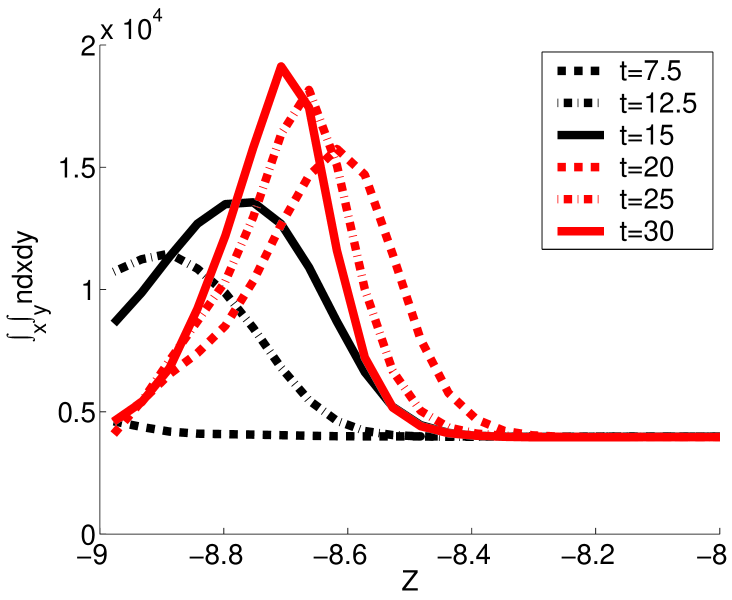
Figure 7:  (Color online) Axial profiles of $\int_{x}\int_{y}ndxdy$ with $v_{\rm inj}=0.09$, $n_{j}/n_{p}=5.13$ (note different than Table 1), and $B_{j}/B_{p}=0$ for jet injected into ITER-like plasma (Table 1), showing shallow deposition of a large number of particles. The “bounce-back” after $t=20$ is due to the open port boundary condition described in Sec. 2.

 

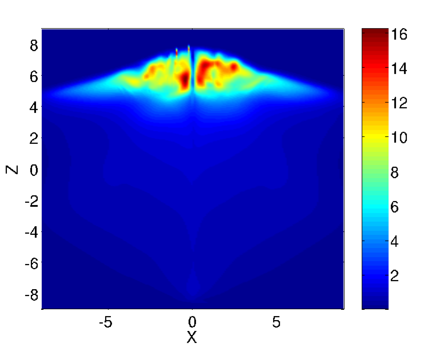
Figure 8: (Color online) Density in the $X$-$Z$ plane with $Y=0$ at $t=25$ ($8.53\,{\rm\mu s}$) for NSTX-relevant parameters of Table 2, showing deep jet penetration. The density structure seen here is characteristic of early time evolution likely due to internal jet mass flow induced by reconnection at the tail. The density smooths out at later times which is the case in Fig. 6.

References

- [1] P. B. Parks. Phys. Rev. Lett., 61:1364, 1988.
- [2] M. Shimada et al. Progress in the ITER Physics Basis Chapter 1: Overview and summary 2007 Nucl. Fusion 47, S1.
- [3] A. V. Voronin, V. K. Gusev, Yu. V. Petrov, N. V. Sakharov, K. B. Abramova, E. M. Sklyarova, and S. Yu. Tolstyakov. Nucl. Fusion, 45:1039, 2005.
- [4] W. Liu, S. C. Hsu, and H. Li. Nucl. Fusion, 49:095008, 2009.
- [5] K. B. Abramova, A. V. Voronin, V. K. Gusev, E. E. Mukhin, Yu. V. Petrov, N. V. Sakharov, and F. V. Chernyshev. Plasma Phys. Rep., 31:721, 2005.
- [6] R. Raman. Fusion Eng Des., 83:1368–1374, 2008.
- [7] S. L. Milora, C. A. Foster, P. H. Edmunds, and G. L. Schmidt. Phys. Rev. Lett., 42, 1979.
- [8] L. J. Perkins, S. K. Ho, and J. H. Hammer. Nucl. Fusion, 28:1365, 1988.
- [9] A. V. Voronin and K. G. Hellblom. Plasma Phys. Control. Fus., 43:1583, 2001.
- [10] F. D. Witherspoon, HyperV Technologies Corp., private communication (2010).
- [11] M. Ono, S. M. Kaye, Y. K. M. Peng, G. Barnes, W. Blanchard, M. D. Carter, J. Chrzanowski, L. Dudek, R. Ewig, D. Gates, R. E. Hatcher, T. Jarboe, S. C. Jardin, D. Johnson, R. Kaita, M. kalish, C. E. Kessel, H. W. Kugel, R. Maingi, R. Majeski, J. Manickam, B. McCormack, J. Menard, D. Mueller, B. A. Nelson, B. E. Nelson, C. Neumeyer, G. Oliaro, F. Paoletti, R. Parsells, E. Perry, N. Pomphrey, S. Ramakrishnan, R. Raman, G. Rewoldt, J. Robinson, A. L. Roquemore, P. Ryan, S. Sabbagh, D. Swain, E. J. Synakowski, M. Viola, M. Williams, and J. R. Wilson. Nucl. Fusion, 40:557, 2000.
- [12] P. T. Lang, B. Alper, R. Buttery, K. Gal, J. Hobirk, J. Neuhauser, and M. Stamp. Nucl. Fusion, 47:754, 2007.
- [13] I. N. Bogatu, S. A. Galkin, and J. S. Kim. J. Fusion Energy, 27:6, 2008.
- [14] W. A. Newcomb. Phys. Fluids B, 3:1818, 1991.
- [15] Y. Suzuki, T.-H Watanabe, T. Sato, and T. Hayashi. Nucl. Fusion, 40:277, 2000.
- [16] Y. Suzuki, T. Hayashi, and Y. Kishimoto. Phys. Plasmas, 7:5033, 2000.
- [17] Y. Suzuki, T. Hayashi, and Y. Kishimoto. Nucl. Fusion, 41:873, 2001.
- [18] V. Rozhansky, I. Senichenkov, I. Veselova, V. Gusev, N. Sakharov, Yu. Petrov, S. Tolstyakov, A. Voronin, and Globus-M team, 33rd EPS Conference on Plasma Physics, 19–23 June 2006, ECA 301, 4.107 (2006).
- [19] H. Li, G. Lapenta, J. M. Finn, S. Li, and S. A. Colgate. Astrophys. J., 643:92–100, 2006.
- [20] D. S. Balsara and D. S. Spicer. J. Comput. Phys., 149:270, 1999.
- [21] D. H. Rudy and J. C. Strikwerda. J. Comp. Phys., 36:55, 1980.
- [22] M. Yamada, R. Kulsrud, and H. Ji. Rev. Mod. Phys., 82:603, 2010.
- [23] G. Olynyk and J. Morelli. Nucl. Fusion, 48:095001, 2008.