Renormalization Group and Conformal Symmetry Breaking in the Chern-Simons Theory Coupled to Matter

Abstract

The three-dimensional Abelian Chern-Simons theory coupled to a scalar and a fermionic field of arbitrary charge is considered in order to study conformal symmetry breakdown and the effective potential stability. We present an improved effective potential computation based on two-loop calculations and the renormalization group equation: the later allows us to sum up series of terms in the effective potential where the power of the logarithms are one, two and three units smaller than the total power of coupling constants (i.e., leading, next-to-leading and next-to-next-to-leading logarithms). For the sake of this calculation we determined the beta function of the fermion-fermion-scalar-scalar interaction and the anomalous dimension of the scalar field. We shown that the improved effective potential provides a much more precise determination of the properties of the theory in the broken phase, compared to the standard effective potential obtained directly from the loop calculations. This happens because the region of the parameter space where dynamical symmetry breaking occurs is drastically reduced by the improvement discussed here.

I Introduction

Chern-Simons (CS) theory DeserJackiwTempleton is an important theoretical framework which has been used to study many issues on quantum field theory in three space-time dimensions. Among the interesting properties of CS theory are the classical conformal invariance and the fact that the gauge field does not receive infinite renormalization, leading to a zero beta function for the gauge coupling constant ChenSemenoff . These are important aspects for the problem of symmetry breaking through radiative corrections CW , which we want to revisit in this work considering a CS theory coupled to matter.

Our study is motivated by some recent developments concerning the summation of the power series in the leading and subleading logarithm terms of the effective potential by means of the renormalization group equation (RGE) elias-charac ; elias-SM . The RGE allows one to obtain extra information from the usual loop approximation, thus providing more refined information concerning quantum properties of the model under scrutiny. An important example where the RGE have dramatically improved the information obtained in the loop approximation is in the analysis of the effective potential for the Standard Model with conformal invariance: from the standard one-loop approximation, the effective action of the model does not seems to be stable, but with the more precise approximation obtained using the RGE, one discover it actually is elias-SM . For other examples see elias-charac ; diasLL ; Meissner ; Nicolai .

We show here an improved calculation of the effective potential of the theory of a CS field coupled to scalar and fermionic fields. The computation includes infinite summations of terms of the effective potential which can be carried out with the RGE and the knowledge of the elements figuring in it: the beta functions, scalar field anomalous dimension and the first logarithm corrections for the effective potential. These elements at lowest approximation need a two-loop calculation to be determined since there are no one-loop divergences in odd space-time dimensions when using the sort of regularization we adopt here (regularization by dimensional reduction). In fact all one particle irreducible diagrams with an odd number of loops will be finite under this scheme. Some of the needed elements were computed in Refs ChenSemenoff ; Hosotani ; avdeev92 ; alves2000 ; diasCS ; in this work, we calculate the fermion anomalous dimension and the beta function for the Yukawa coupling.

A peculiarity of CS theory has to be mentioned at this point. The theory involves the Levi-Civita tensor which cannot be easily extended to arbitrary dimensions as needed in the context of dimensional regularization. A regularization procedure called dimensional reduction siegel has been shown to be appropriated in dealing with CS theory ChenSemenoff ; avdeev92 ; alves2000 : essentially, it consists in performing the tensor and gamma matrices algebra in three dimensions, and extending only the momentum integrals to arbitrary dimensions.

The two-loop results, in conjunction with the RGE, allows us to sum up all terms in the effective potential where the total power of the coupling constants is one and two units larger than the power of the logarithms $\log\left(\phi/\mu^{2}\right)$ (called leading logarithms, LL, and next-to-leading logarithms, NLL, terms), as well as some subseries where they are three units larger (the next-to-next-to-leading logarithms terms). We study the dynamical symmetry breaking of the conformal symmetry in this theory, showing that the improved effective potential leads to a much finer determination of the properties in the broken phase, such as mass and coupling constant of the scalar field. This happens because the region of the parameter space of the theory, where the dynamical breaking of symmetry is operational at the perturbative level, is much smaller when considering the improved effective potential than for the initial two-loop potential. Another interesting aspect is that, for certain values of the parameters, we found two broken vacua, which leads to different physical properties. This happens both for the improved and the original effective potential, but the region of the parameter space where this happens is much more restricted for the former case. Again, the improvement of the perturbative effective potential calculation provides more precise determination of the properties of the theory.

We believe that the outcomes of our analysis involving the Chern-Simons theory enforces the idea that one has to extract the maximum amount of information from a given perturbative calculation, by using the renormalization group equations to obtain a better approximation to the effective potential. Even if its natural at a first moment to use one-loop results to predict masses and coupling constants from any of the many proposed extensions to the Standard Model, for example, one should enrich the analysis of the dynamical symmetry breaking by means of the RGE.

This paper is organized as follows. The method of using the RGE to sum up series of perturbative corrections to the effective potential is outlined in Sec. II. The model we shall study is described in Sec. III. Technical details of the two-loop calculations needed for this work are presented in Sec. IV. Sec. V contains the detailed calculation of the improved effective potential, which is used to study the dynamical breaking of the conformal symmetry in Sec. VI. Finally, our conclusions are summarized in Sec. VII.

II General Considerations

We start by reviewing the use of the RGE to calculate the improved effective potential. As discussed in elias-charac , the standard practice for solving the RGE by replacing the couplings in the effective potential by their running values amounts to a particular application of the method of characteristics to solve partial differential equations. This procedure does not exhaust, however, the information that is contained in the RGE: actually, a finer approximation can be obtaining by writing the effective potential as a general power series in the couplings and logarithms of the scalar field, and using the RGE to sum up some infinite subsets of this power series.

To explain the general procedure, we will consider a general model of a scalar field $\varphi$ with a self-interaction of the form $\varphi^{N}$, together with interactions with other dynamical fields. As known, in three spacetime dimensions, renormalizability imposes that $N\leq 6$, but we shall not fix any particular value of $N$ in this Section. Let $\lambda=\left\{\lambda_{i},\,i=1,\ldots M\right\}$ denote collectively the set of all coupling constants of the theory. The RGE for the regularized effective potential $V_{\mbox{eff}}\left(\phi\right)$ reads

$$\left[\mu\frac{\partial}{\partial\mu}+\beta_{\lambda}\frac{\partial}{\partial\lambda}-\gamma_{\varphi}\phi\frac{\partial}{\partial\phi}\right]V_{\mbox{eff}}\left(\phi;\mu,\varepsilon,\lambda,L\right)=0\,$$ (1)

(in this section, the sum over all $\lambda_{i}$ will always be implicit). Here, $\mu$ is the arbitrary mass scale introduced when we use dimensional regularization to extended the theory to dimension $D$, $\gamma_{\varphi}$ is the anomalous dimension of the scalar $\varphi$, $\varepsilon=3-D$,

$$L=\ln\frac{\phi^{2}}{\mu}\,,$$ (2)

and $\phi$ is the vacuum expectation value of the scalar field $\varphi$.

For the sake of convenience, we introduce the notation (from now on, we omit the explicit dependence on the parameters $\mu,\varepsilon,\lambda,L$),

$$V_{\mbox{eff}}\left(\phi\right)=\phi^{N}S_{\mbox{eff}}\left(\phi\right)\,,$$ (3)

where $S_{\mbox{eff}}\left(\phi\right)$, on very general grounds, is a sum of terms involving different powers of $\lambda$ and $L$, which in principle can be calculated order by order in the loop expansion.

In order to use the RGE we shall organize the terms in $S_{\mbox{eff}}\left(\phi\right)$ according to the power of $L$ relative to the aggregate powers of the couplings $\lambda$, i.e.,

$$S_{\mbox{eff}}\left(\phi\right)=S_{\mbox{eff}}^{{\rm LL}}\left(\phi\right)+S_{\mbox{eff}}^{{\rm NLL}}\left(\phi\right)+S_{\mbox{eff}}^{{\rm N2LL}}\left(\phi\right)+\cdots\,,$$ (4)

where

$$S_{\mbox{eff}}^{{\rm LL}}\left(\phi\right)=\sum_{n\geq 1}C_{n}^{{\rm LL}}\lambda^{n}L^{n-1}\,,$$ (5)

is the sum of the leading logarithms in $S_{\mbox{eff}}\left(\phi\right)$, and

$$S_{\mbox{eff}}^{{\rm NLL}}\left(\phi\right)=\sum_{n\geq 3}C_{n}^{{\rm NLL}}\lambda^{n}L^{n-2}\,,$$ (6)

$$S_{\mbox{eff}}^{{\rm N2LL}}\left(\phi\right)=\sum_{n\geq 3}C_{n}^{{\rm N2LL}}\lambda^{n}L^{n-3}\,,$$ (7)

are the next-to-leading and next-to-next-to-leading logarithms terms, respectively; here, $\lambda^{n}=\prod\lambda_{i}^{n_{i}}$ with $\sum n_{i}=n$. The RGE allows one to calculate these sums once their first coefficient is known, if we have enough information on the $\beta$-functions and the anomalous dimension of the scalar field. To see how this come about, we use the definition (3) in Eq. (1), and take Eq. (2) into account to rewrite the RGE in a more convenient form,

$$\left[-\left(1+2\gamma_{\phi}\right)\frac{\partial}{\partial L}+\beta_{\lambda}\frac{\partial}{\partial\lambda}-N\gamma_{\varphi}\right]S_{\mbox{eff}}\left(\phi;\mu,\varepsilon,\lambda,L\right)=0\,.$$ (8)

We shall write $\gamma_{\varphi}$ and $\beta_{\lambda}$ in the form

$$\gamma_{\varphi} =\gamma_{\varphi}^{\left(2\right)}+\gamma_{\varphi}^{\left(3\right)}+\cdots\,,$$ (9)

$$\beta_{\lambda} =\beta_{\lambda}^{\left(2\right)}+\beta_{\lambda}^{\left(3\right)}+\cdots\,,$$ (10)

where $\gamma_{\varphi}^{\left(j\right)}$ and $\beta_{\lambda}^{\left(j\right)}$ denotes the terms of order $\lambda^{j}$ of the anomalous dimension and beta function, respectively; these can be obtained by explicit loop calculations.

Substituting the expansion (4) in (8) we find, at the leading order (terms proportional to $\lambda^{n}L^{n-2}$),

$$\left[-\frac{\partial}{\partial L}+\beta_{\lambda}^{\left(2\right)}\frac{\partial}{\partial\lambda}\right]S_{\mbox{eff}}^{{\rm LL}}\left(\phi\right)=0\,.$$ (11)

This results in a first order difference equation for the coefficients $C_{n}^{{\rm LL}}$; in this way $S_{\mbox{eff}}^{{\rm LL}}\left(\phi\right)$ can be determined once we know $\beta_{\lambda}^{\left(2\right)}$ and the initial coefficient $C_{1}^{{\rm LL}}$. Having $S_{\mbox{eff}}^{{\rm LL}}\left(\phi\right)$ at our disposal, we can focus at terms of order $\lambda^{n}L^{n-3}$ in (8),

$$\left[-\frac{\partial}{\partial L}+\beta_{\lambda}^{\left(2\right)}\frac{\partial}{\partial\lambda}\right]S_{\mbox{eff}}^{{\rm NLL}}\left(\phi\right)+\left[\beta_{\lambda}^{\left(3\right)}\frac{\partial}{\partial\lambda}-N\gamma_{\varphi}^{\left(2\right)}\right]S_{\mbox{eff}}^{{\rm LL}}\left(\phi\right)=0\,.$$ (12)

Since $S_{\mbox{eff}}^{{\rm LL}}\left(\phi\right)$ is known, this equation allows us to calculate $S_{\mbox{eff}}^{{\rm NLL}}\left(\phi\right)$ if we have $\beta_{\lambda}^{\left(3\right)}$, $\gamma_{\varphi}^{\left(2\right)}$ and $C_{2}^{{\rm NLL}}$.

This procedure can be repeated until we have exhausted the information on $\beta_{\lambda}$, $\gamma_{\varphi}$ and the initial coefficients $C$ from the explicit loop calculations. In summary, the RGE allows one to use the knowledge of $S_{\mbox{eff}}\left(\phi\right)$, $\beta_{\lambda}$ and $\gamma_{\varphi}$ up to a given loop order to sum up complete subsets of contributions for the effective potential arising from all loop orders, thus extracting the maximum amount of information from our perturbative calculation.

III The Model

We shall now consider a Chern-Simons field $A_{\mu}$ in three spacetime dimensions coupled to a two component Dirac field $\psi$ and a complex scalar field $\varphi$, both charged under the $U\left(1\right)$ gauge symmetry of the CS field according to the Lagrangian

$$\mathcal{L}= \frac{1}{2}\epsilon_{\mu\nu\rho}A^{\mu}\partial^{\nu}A^{\rho}+i\overline{\psi}\gamma^{\mu}D_{\mu}\psi+\left(D^{\mu}\varphi\right)^{\dagger}\left(D_{\mu}\varphi\right)$$ (13)

$$-\frac{\nu}{6}\left(\varphi^{\dagger}\varphi\right)^{3}-\alpha\varphi^{\dagger}\varphi\overline{\psi}\psi\,.$$

The theory has a self-interaction for the scalar field and an Yukawa-like interaction between scalar and fermions fields. In Eq. (13), $\nu$ is a positive coupling constant and $D^{\mu}=\partial^{\mu}-ienA^{\mu}$, where $n$ is the charge of the field $D^{\mu}$ is acting on. Without loss of generality, we can consider $n_{\varphi}=1$, since any $n_{\varphi}\neq 1$ can be reabsorbed by a redefinition of the gauge coupling constant $e$. Therefore, we will denote simply by $n$ the charge of the fermion, from now on. The spacetime metric is $g^{\mu\nu}=(1,-1,-1)$, the fully antisymmetric Levi-Civita tensor $\epsilon_{\mu\nu\rho}$ is normalized as $\epsilon_{012}=1$, and the gamma matrices were chosen as $\gamma^{\mu}=\left(\sigma^{3},i\sigma^{1},i\sigma^{2}\right)$.

The Lagrangian in Eq. (13) is a $\left(2+1\right)$ dimensional analog of the well known Coleman-Weinberg model in $(3+1)$ dimensions CW , in the sense that all parameters appearing in the classical Lagrangian are dimensionless, so it posseses classical conformal invariance. As we assume such an invariance at the classical level, to deal with quantum corrections it is appropriate to use a regularization method that violates it minimally meissner2007 . The observations made in meissner2007 regarding dimensional regularization are straightforwardly generalized for regularization by dimensional reduction, which has been used to obtain the quantities we need here. Divergent integrals are regulated by the replacement $\int d^{3}k/(2\pi)^{3}\rightarrow\mu^{\epsilon}\int d^{3-\epsilon}k/(2\pi)^{3-\epsilon}$, where the mass scale $\mu$ is introduced to keep the dimensions of the relevant quantities unchanged. Conformal invariance is broken explicitly by this mass scale, but $\mu$ comes with the evanescent exponent $\epsilon$ and this, in conjunction with the poles $1/\epsilon$, means that $\mu$ always appears inside a logarithm. Also, regularization by dimensional reduction has been shown to preserve Ward identities at least until the two loop order alves2000 ; dias2001 .

Details of the two-loop calculation of the effective potential for a theory like in eq. (13) can be found in diasCS . In summary, after introducing a convenient gauge fixing, one defines a Lagrangian $\hat{\mathcal{L}}_{\mbox{int}}$ shifting the scalar fields by a constant, and disregarding terms independent of or linear on the fields jackiw74 ; after that, the effective potential can be calculated by means of

$$V_{\mbox{eff}}\left(\phi\right)=\frac{\nu}{48}\phi^{6}-\frac{i}{2}\int\frac{d^{3}\hskip 2.84544ptk}{(2\pi)^{3}}\ln\left[\det\left(i\Delta_{\alpha\beta}^{-1}\left(k,\phi_{i}\right)\right)\right]+i<0|\,T\exp i\!\int d^{3}x\,\hat{\mathcal{L}}_{\mbox{int}}|0>.$$ (14)

Hereafter, $\phi^{2}$ stands for $\sqrt{2}\left\langle\varphi^{\dagger}\varphi\right\rangle$. The first and second terms in Eq. (14) are, respectively, the tree approximation and the one-loop correction to the effective potential; the third term is the sum of the vacuum diagrams with two and more loops.

We quote here the two-loop effective potential in the following form diasCS ,

$$V_{\mbox{eff}}^{2\ell}\left(\phi\right)=\frac{\pi}{6}\phi^{6}S_{\mbox{eff}}^{2\ell}\left(\phi\right)\,,$$ (15)

where $S_{\mbox{eff}}^{2\ell}\left(\phi\right)$ is more conveniently written in terms of the coupling constants

$$y=\frac{\nu}{8\pi^{2}}\,\,;\,\,x=\frac{e^{2}}{2\pi}\,\,;\,\,z=\frac{\alpha}{2\pi}\,,$$ (16)

as follows,

$$S_{\mbox{eff}}^{2\ell}\left(\phi\right)\,=\,y+ \left[24\left(1+\frac{n_{\psi}^{2}}{8}\right)x^{4}-\frac{33}{2}x^{2}y+14y^{2}+\right.$$

$$\left.\frac{15}{4}yz^{2}-3z^{4}-6n_{\psi}^{2}x^{3}z+3n_{\psi}^{2}x^{2}z^{2}\right]L\,.$$ (17)

On the other hand, as discussed in Section II, the general form for $S_{\mbox{eff}}\left(\phi\right)$ can be cast as in Eq. (4), with

$$S_{\mbox{eff}}^{{\rm LL}}\left(\phi\right) =\underset{\left(n+m+p\geq 1\right)}{\sum_{n,m,p\geq 0}}C_{n,m,p}^{{\rm LL}}x^{n}y^{m}z^{p}L^{n+m+p-1}$$ (18)

$$S_{\mbox{eff}}^{{\rm NLL}}\left(\phi\right)=\underset{\left(n+m+p\geq 2\right)}{\sum_{n,m,p\geq 0}}C_{n,m,p}^{{\rm NLL}}x^{n}y^{m}z^{p}L^{n+m-2}\,,$$ (19)

and

$$S_{\mbox{eff}}^{{\rm N2LL}}\left(\phi\right)=\underset{\left(n+m+p\geq 3\right)}{\sum_{n,m,p\geq 0}}C_{n,m,p}^{{\rm N2LL}}x^{n}y^{m}z^{p}L^{n+m-3}\,.$$ (20)

It is known that the beta function of the gauge coupling $x$ vanishes in CS model coupled to scalar and fermionic fields ChenSemenoff ; we calculate the two-loop approximation the beta function $\beta_{\alpha}$ of the Yukawa coupling, as well as the scalar anomalous dimension $\gamma_{\varphi}$ in Section IV. The Renormalization Group equation reads, in our model,

$$\left[-\left(1+2\gamma_{\phi}\right)\frac{\partial}{\partial L}+\beta_{y}\frac{\partial}{\partial y}+\beta_{z}\frac{\partial}{\partial z}-6\gamma_{\varphi}\right]S_{\mbox{eff}}\left(\phi\right)=0\,.$$ (21)

By following the procedure outlined in Section II, we obtained closed-form expressions for $S_{\mbox{eff}}^{{\rm LL}}\left(\phi\right)$, $S_{\mbox{eff}}^{{\rm NLL}}\left(\phi\right)$ and $S_{\mbox{eff}}^{{\rm N2LL}}\left(\phi\right)$. The technical details of this calculation are quite involved and are developed in Section V. The results we obtain are the following,

$$S_{\mbox{eff}}^{{\rm LL}}\left(\phi\right) =\frac{y}{w}\,,$$ (22a)

$$S_{\mbox{eff}}^{{\rm NLL}}\left(\phi\right) =x^{2}S_{\left(2,0\right)}^{{\rm NLL}}\left(w\right)+z^{2}S_{\left(0,2\right)}^{{\rm NLL}}\left(w\right)\,,$$ (22b)

$$S_{\mbox{eff}}^{{\rm N2LL}}\left(\phi\right)= \left(x^{4}S_{\left(4,0\right)}^{{\rm N2LL}}\left(w\right)+z^{4}S_{\left(0,4\right)}^{{\rm N2LL}}\left(w\right)\right.$$

$$\left.+x^{2}z^{2}S_{\left(2,2\right)}^{{\rm N2LL}}\left(w\right)+x^{3}zS_{\left(3,1\right)}^{{\rm N2LL}}\left(w\right)\right)L\,,$$ (22c)

where

$$w=1-a_{1}yL$$ (23)

and the functions of $w$ appearing in Eq. (22) are explicitly displayed in Section V.

IV Two-loop wavefunction renormalization and $\beta$ functions

For the purposes of this work we need to calculate the beta function for the Yukawa coupling $\alpha\varphi^{\dagger}\varphi\overline{\psi}\psi$, which implies in calculating the renormalization of the four-point $\varphi^{\dagger}\varphi\overline{\psi}\psi$ function, as well as the wave function renormalization of the $\psi$ field. To evaluate these quantities, we calculated in the two-loop approximation the divergent parts of the fermion two-point vertex-function $\Gamma_{\overline{\psi}\psi}$ and the four point vertex function $\Gamma_{\varphi^{\dagger}\varphi\overline{\psi}\psi}$. Free propagators for fermionic, scalar and gauge fields are given respectively by

$$\Delta_{\psi}\left(k\right) =\frac{i}{\not{k}-i\eta}\,,$$ (24a)

$$\Delta_{\varphi}\left(k\right) =\frac{i}{k^{2}-i\eta}\,,$$ (24b)

$$\Delta_{\mu\nu}\left(k\right) =\frac{\varepsilon_{\mu\nu\sigma}k^{\sigma}}{k^{2}-i\eta}\,,$$ (24c)

while the elementary vertices are

$$\mbox{trilinear }\overline{\psi}\psi A_{\rho} \leftrightarrow -ie\gamma_{\rho}\mu^{\varepsilon/2}\,,$$ (25a)

$$\mbox{trilinear }\overline{\varphi}\left(p\right)\varphi\left(-q\right)A_{\rho} \leftrightarrow -ie\left(p+q\right)_{\rho}\mu^{\varepsilon/2}\,,$$ (25b)

$$\mbox{quadrilinear }\overline{\varphi}\varphi A_{\rho}A_{\sigma} \leftrightarrow ie^{2}g_{\rho\sigma}\mu^{\varepsilon}\,,$$ (25c)

$$\mbox{quadrilinear }\overline{\psi}\psi\overline{\varphi}\varphi \leftrightarrow -i\alpha\mu^{\varepsilon}\,,$$ (25d)

where, in the $\overline{\varphi}\varphi A$ vertex, the indicated momenta are the ones entering the respective line.

The diagrams involved in calculating the two-point vertex function of the fermion are shown in Fig. 1, and the corresponding divergent parts are given by,

$$\left(a\right) =-\frac{\alpha^{2}}{6}\,,\,\,\left(b\right)=\left(c\right)=\frac{5e^{4}}{36}\,,$$ (26a)

$$\left(d\right) =-\frac{e^{4}}{3}\,,\,\,\left(e\right)=\frac{e^{4}}{2}\,,$$ (26b)

apart from an $\left(i\mu^{2\varepsilon}/16\pi^{2}\right)\not{k}/\varepsilon$ factor.

We also evaluated the divergent part of the four-point $\overline{\psi}\psi\overline{\varphi}\varphi$ vertex function in the two-loop approximation. Our method for this calculation was the following one: all two-loop 1PI diagrams for such vertex function were generated using the Mathematica package FeynArts feynarts , resulting in about 200 diagrams The identification of the divergent diagrams was greatly facilitated by the fact that, for the purpose of evaluating the divergent part of the $\overline{\psi}\psi\overline{\varphi}\varphi$ function, we could calculate the diagrams with vanishing external momenta. This allowed us to prove an important rule, all diagrams with a trilinear $\overline{\varphi}\varphi A$ vertex attached to an external line are finite due to the antisymmetry of the gauge propagator $\Delta_{\mu\nu}$. This rule is graphically represented in Fig. 2. There are also some one-loop diagrams that vanish (those depicted in Fig. 3) and appear as subdiagrams of some of the initial set. Using the pattern-matching capabilities of Mathematica, we could use such rules to narrow down the set of possibly divergent two-loop diagrams to those appearing in Fig. 4. The result of the calculation of these diagrams appears in Table 1.

With these results, we can now write down the relation between bare (denoted by the subscript zero) and renormalized fields and coupling constants

$$\varphi_{0} =Z_{\varphi}^{\frac{1}{2}}\varphi=\left(1+A\right)^{\frac{1}{2}}\varphi\,,$$ (27a)

$$\psi_{0} =Z_{\psi}^{\frac{1}{2}}\psi=\left(1+F\right)^{\frac{1}{2}}\psi\,,$$ (27b)

$$\alpha_{0}\overline{\varphi}_{0}\varphi_{0}\overline{\psi}_{0}\psi_{0} =\mu^{\varepsilon}\left(\alpha+\delta\alpha\right)\overline{\varphi}\varphi\overline{\psi}\psi\,.$$ (27c)

The constant $Z_{\varphi}$ has already been calculated in diasCS , and the results of Eq. (26) and Table 1 allow us to find $Z_{\psi}$ and $\delta\alpha$:

$$\delta\alpha =-\frac{1}{32\pi^{2}\varepsilon}\left(7e^{4}\alpha+4e^{2}\alpha^{2}+20e^{6}-4\alpha^{3}\right)\,,$$ (28a)

$$Z_{\psi} =1+\frac{1}{288\pi^{2}\varepsilon}\left(3\alpha^{2}-8e^{8}\right)\,,$$ (28b)

$$Z_{\varphi} =1+\frac{1}{16\pi^{2}\varepsilon}\left[\frac{e^{4}}{3}(7+2n^{2})-\frac{\alpha^{2}}{6}\right]\,.$$ (28c)

The beta function for the Yukawa coupling is calculated from the relation (27c)

$$\alpha_{0}=\frac{\mu^{\varepsilon}\left(\alpha+\delta\alpha\right)}{Z_{\psi}Z_{\varphi}}\,,$$ (29)

since $d\alpha_{0}/d\mu=0$, we have

$$\beta_{\alpha}=\mu\frac{d\alpha}{d\mu}=\frac{1}{8\pi^{2}}\left[5e^{6}+\left(\frac{97}{36}+\frac{n^{2}}{3}\right)\alpha e^{4}+\alpha^{2}e^{2}-\alpha^{3}\right]\,.$$ (30)

In terms of the rescaled coupling constants in Eq. (16),

$$\beta_{z}=\frac{\beta_{\alpha}}{2\pi}=\frac{5}{2}x^{3}+\left(\frac{97}{72}+\frac{n^{2}}{6}\right)zx^{2}+\frac{1}{2}z^{2}x-\frac{1}{2}z^{3}\,.$$ (31)

From Eqs. (28b) and (28c), we obtain the anomalous dimensions for scalar and fermion fields,

$$\gamma_{\varphi} =-\frac{1}{Z_{\varphi}}\frac{dZ_{\varphi}}{\mu}=-\left(\frac{7}{12}+\frac{n^{2}}{6}\right)x^{2}+\frac{1}{24}z^{2}\,,$$ (32a)

$$\gamma_{\psi} =-\frac{1}{Z_{\psi}}\frac{dZ_{\psi}}{\mu}=-\frac{1}{9}x^{2}+\frac{1}{24}z^{2}\,,$$ (32b)

where $\gamma_{\psi}$ has been quoted just for completeness.

As for the beta function of the coupling $\nu$, it is most easily calculated by relating it with the effective potential in Eq. (17) and the anomalous dimension $\gamma_{\varphi}$ by means of the renormalization group equation, as done in diasCS . Here, we just quote the result, taking into account Eq. (16) and the fact that the fermion has charge $n$,

$$\beta_{y}= 24\left(1+\frac{n^{2}}{8}\right)x^{4}-\left(n^{2}+20\right)x^{2}y+14y^{2}$$ (33)

$$+4yz^{2}-3z^{4}-6n^{2}x^{3}z+3n^{2}x^{2}z^{2}.$$ (34)

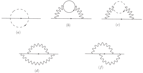
Figure 1: Two-loop contributions to the fermion two-point vertex function.

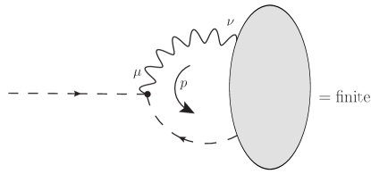
Figure 2: A simple rule for establishing the finiteness of a subset of diagrams: since the external momenta can be taken to zero, whenever there is a trilinear $\overline{\varphi}\varphi A$ vertex attached to an external line, the resulting Feynman integrand would contain a factor $\Delta_{\mu\nu}\times\left(-iep^{\mu}\right)$, thus vanishing due to the antisymmetry of the gauge propagator $\Delta_{\mu\nu}$.

Figure 3: One-loop vanishing diagrams that appear as subgraphs of some of the two-loop contributions to the four-point vertex function.

Figure 4: Potentially divergent two-loop diagrams.

D1	$-\frac{3}{2}\alpha e^{4}$	D6	$-e^{6}$	D11	$\frac{1}{2}\alpha^{3}$	D16	$-\alpha e^{4}$	D21	$-e^{6}$
D2	$0$	D7	$\alpha e^{4}$	D12	$\frac{1}{4}\alpha^{3}$	D17	$\frac{1}{2}\alpha^{2}e^{2}$	D22	$-\frac{1}{4}\alpha e^{4}$
D3	$-\alpha^{2}e^{2}$	D8	$\frac{1}{2}\alpha e^{4}$	D13	$-\frac{1}{2}\alpha e^{4}$	D18	$0$	D23	$-\alpha e^{4}$
D4	$\alpha e^{4}$	D9	$e^{6}$	D14	$-\frac{1}{2}\alpha^{2}e^{2}$	D19	$-\frac{1}{4}\alpha e^{4}$	D24	$-e^{6}$
D5	$\frac{1}{2}\alpha e^{4}$	D10	$\frac{1}{4}\alpha^{3}$	D15	$-2e^{6}$	D20	$-\frac{1}{4}\alpha e^{4}$	D25	$-e^{6}$

Table 1: Divergent parts of the diagrams appearing in Fig. 4, omitting an overall factor of $i\mu^{\varepsilon}/8\pi^{2}\varepsilon$.

V Calculation of the Improved Effective Potential

In this Section, we apply the methodology outlined in Section II to the present theory. We use as a starting point the two-loop effective potential in Eq. (17), from which one can identify the numerical values of the initial $C_{m,n,p}$ coefficients of the expansion

$$S_{\mbox{eff}}\left(\phi\right) =\sum_{n,m,p\geq 0}C_{n,m,p}^{{\rm LL}}x^{n}y^{m}z^{p}L^{n+m+p-1}$$

$$+\sum_{n,m,p\geq 0}C_{n,m,p}^{{\rm NLL}}x^{n}y^{m}z^{p}L^{n+m+p-2}$$

$$+\sum_{n,m,p\geq 0}C_{n,m,p}^{{\rm N2LL}}x^{n}y^{m}z^{p}L^{n+m+p-3}+\cdots\,,$$ (35)

by casting Eq. (17) as

$$S_{\mbox{eff}}^{2\ell}\left(\phi\right)= y\left(C_{0,1,0}^{{\rm LL}}+C_{0,2,0}^{{\rm LL}}yL\right)+\left(x^{2}C_{2,1,0}^{{\rm NLL}}yL+z^{2}C_{0,1,2}^{{\rm NLL}}\right)yL$$

$$+\left(C_{4,0,0}^{{\rm N2LL}}x^{4}+C_{0,0,4}^{{\rm N2LL}}z^{4}+C_{3,0,1}^{{\rm N2LL}}x^{3}z+C_{2,0,2}^{{\rm N2LL}}x^{2}z^{2}\right)L\,.$$ (36)

The beta functions and anomalous dimension that appears in the RGE,

$$\left[-\left(1+2\gamma_{\phi}\right)\frac{\partial}{\partial L}+\beta_{y}\frac{\partial}{\partial y}+\beta_{z}\frac{\partial}{\partial z}-6\gamma_{\varphi}\right]S_{\mbox{eff}}\left(\phi\right)=0\,;$$ (37)

were presented in Section IV, and can be cast as

$$\beta_{y} =\beta_{y}^{\left(2\right)}+\beta_{y}^{\left(3\right)}+\beta_{y}^{\left(4\right)}\,,$$ (38)

where

$$\beta_{y}^{\left(2\right)} =a_{1}y^{2}\,\,;\,\,\beta_{y}^{\left(3\right)}=a_{2}x^{2}y+a_{3}yz^{2}\,,$$

$$\beta_{y}^{\left(4\right)} =a_{4}x^{4}+a_{5}z^{4}+a_{6}x^{3}z+a_{7}x^{2}z^{2}\,,$$ (39)

and

$$\beta_{z}=\beta_{z}^{\left(3\right)}=b_{1}z^{3}+b_{2}z^{2}x+b_{3}zx^{2}+b_{4}x^{3}\,,$$ (40)

as for the anomalous dimension, we have

$$\gamma_{\varphi} =\gamma_{\varphi}^{\left(2\right)}=c_{1}x^{2}+c_{2}z^{2}\,.$$ (41)

The numerical values of the coefficients appearing in the last equations are

$$a_{1} =14,\;a_{2}=6c_{1}-\frac{33}{2}=-\left(n^{2}+20\right),$$ (42a)

$$a_{3} =6c_{2}+\frac{15}{4}=4,\,a_{4}=24\left(1+\frac{n^{2}}{8}\right)\,,$$ (42b)

$$a_{5} =-3,\;a_{6}=-6n^{2},\;a_{7}=3n^{2}\,,$$ (42c)

$$c_{1} =-\left(\frac{7}{12}+\frac{n^{2}}{6}\right),\;c_{2}=\frac{1}{24}\,,$$ (42d)

$$b_{1} =-\frac{1}{2},\,b_{2}=\frac{1}{2},\,b_{3}=\frac{97}{72}+\frac{n^{2}}{6},\,b_{4}=\frac{5}{2}$$ (42e)

where $n$ is the charge of the fermionic field.

Using these results, we can split Eq. (37) according to the relative powers of coupling constants and logarithms,

$$\left[-\frac{\partial}{\partial L}+\beta_{y}^{\left(2\right)}\frac{\partial}{\partial y}\right]S_{\mbox{eff}}^{{\rm LL}}$$

$$+\left\{\left[\beta_{y}^{\left(3\right)}\frac{\partial}{\partial y}+\beta_{z}^{\left(3\right)}\frac{\partial}{\partial z}-6\gamma_{\varphi}^{\left(2\right)}\right]S_{\mbox{eff}}^{{\rm LL}}+\left[-\frac{\partial}{\partial L}+\beta_{y}^{\left(2\right)}\frac{\partial}{\partial y}\right]S_{\mbox{eff}}^{{\rm NLL}}\right\}$$

$$+\left\{\left[-2\gamma_{x}^{\left(2\right)}\frac{\partial}{\partial L}+\beta_{y}^{\left(4\right)}\frac{\partial}{\partial y}\right]S_{\mbox{eff}}^{{\rm LL}}+\left[\beta_{y}^{\left(3\right)}\frac{\partial}{\partial y}+\beta_{z}^{\left(3\right)}\frac{\partial}{\partial z}-6\gamma_{\varphi}^{\left(2\right)}\right]S_{\mbox{eff}}^{{\rm NLL}}+\left[-\frac{\partial}{\partial L}+\beta_{y}^{\left(2\right)}\frac{\partial}{\partial y}\right]S_{\mbox{eff}}^{{\rm N2LL}}\right\}$$

$$=0$$ (43)

V.1 Leading logarithms

Focusing first on terms of order $x^{m}y^{n}z^{p}L^{n+m+p-2}$ in Eq. (43), one obtains

$$\left[-\frac{\partial}{\partial L}+\beta_{y}^{\left(2\right)}\frac{\partial}{\partial y}\right]S_{\mbox{eff}}^{{\rm LL}}\left(\phi\right) =$$

$$\left[-\frac{\partial}{\partial L}+a_{1}y^{2}\frac{\partial}{\partial y}\right] \underset{\left(m+n+p\geq 1\right)}{\sum_{m,n,p}}C_{m,n,p}^{{\rm LL}}x^{m}y^{n}z^{p}L^{m+n+p-1}=0$$ (44)

which furnishes the following relation for the coefficients $C_{n,m,p}^{{\rm LL}}$,

$$\left(m+n+p-1\right)C_{m,n,p}^{{\rm LL}}-\left(n-1\right)a_{1}C_{m,n-1,p}^{{\rm LL}}=0\quad\left(m+n+p\geq 2\right)\,.$$ (45)

We find convenient to recast $S_{\mbox{eff}}^{{\rm LL}}\left(\phi\right)$ as

$$S_{\mbox{eff}}^{{\rm LL}}\left(\phi\right)= yS_{\left(0\right)}^{{\rm LL}}\left(u\right)+\sum_{m+p\geq 1}x^{m}z^{p}L^{m+p-1}S_{\left(m,p\right)}^{{\rm LL}}\left(u\right)\,,$$ (46)

where

$$S_{\left(0\right)}^{{\rm LL}}\left(u\right)= \sum_{n\geq 0}C_{0,n+1,0}^{{\rm LL}}u^{n},$$ (47)

$$S_{\left(m,p\right)}^{{\rm LL}}\left(u\right)= \sum_{n\geq 0}C_{m,n,p}^{{\rm LL}}u^{n},$$ (48)

in terms of the variable $u=yL$. Inspection of Eq. (17) allows one to find the initial coefficient of these sums,

$$C_{0,1,0}^{LL} =1,\quad C_{0,2,0}^{LL}=a_{1}\,,$$

$$C_{1,0,0}^{LL} =C_{0,0,1}^{LL}=C_{1,1,0}^{LL}=C_{1,0,1}^{LL}=C_{0,1,1}^{LL}=C_{2,0,0}^{LL}=C_{0,0,2}^{LL}=0\,.$$ (49)

By looking at Eq. (45) with $m=p=0$, we have

$$C_{0,n,0}^{{\rm LL}}=a_{1}C_{0,n-1,0}^{{\rm LL}}\quad\left(n\geq 2\right)\,,$$ (50)

with, together with the values $C_{0,1,0}^{LL},C_{0,2,0}^{LL}$ from Eq. (49), leads to

$$C_{0,n,0}^{{\rm LL}}=a_{1}^{n-1}\quad\left(n\geq 1\right)$$ (51)

hence,

$$S_{\left(0\right)}^{{\rm LL}}\left(u\right)=\sum_{n\geq 0}a_{1}^{n}u^{n}=\frac{1}{1-a_{1}u}\,.$$ (52)

Now setting $m=1$ and $p=0$ in Eq. (45),

$$nC_{1,n,0}^{{\rm LL}}-\left(n-1\right)a_{1}C_{1,n-1,0}^{{\rm LL}}=0\quad\left(n\geq 1\right)\,,$$ (53)

and from this equation one concludes that $C_{1,1,0}^{{\rm LL}}=0$, which is consistent with the results obtained from the two-loop calculation of $V_{\mbox{eff}}$ in Eq. (49); this is an important consistency check of that result. Also from Eq. (53), by recurrence we have

$$C_{1,n,0}^{{\rm LL}}=0\quad\left(n\geq 0\right)\,,$$ (54)

so that $S_{\left(1,0\right)}^{{\rm LL}}\left(u\right)=0$. Similar results are found by setting $m=0$ and $p=1$, i.e.,

$$C_{0,n,1}^{{\rm LL}}=0\quad\left(n\geq 0\right)\,,$$ (55)

thus $S_{\left(0,1\right)}^{{\rm LL}}\left(u\right)=0$.

Now looking at the terms with $m+p\geq 2$ in Eq. (45), for $n=1$ we immediately obtain

$$C_{m,1,p}^{{\rm LL}}=0\,,$$ (56)

which, by recurrence for larger $n$, implies that

$$C_{m,n,p}^{{\rm LL}}=0\,.\quad\left(m+p\geq 2\right)$$ (57)

Summarizing this results,

$$S_{\left(m,p\right)}^{{\rm LL}}\left(u\right)=0\quad\left(m,p\neq 0\right)\,,$$ (58)

therefore,

$$S_{\mbox{eff}}^{{\rm LL}}\left(\phi\right)=yS_{\left(0\right)}^{{\rm LL}}\left(u\right)=\frac{y}{w}\,,$$ (59)

where we have introduced the definition

$$w=1-a_{1}u=1-a_{1}yL\,.$$ (60)

V.2 Next-to-leading logarithms

Having found $S_{\mbox{eff}}^{{\rm LL}}$, we can now consider terms of order $x^{m}y^{n}z^{p}L^{m+n+p-3}$ in Eq. (43),

$$\left[\beta_{y}^{\left(3\right)}\frac{\partial}{\partial y}+\beta_{z}^{\left(3\right)}\frac{\partial}{\partial z}-6\gamma_{\varphi}^{\left(2\right)}\right]S_{\mbox{eff}}^{{\rm LL}}+\left[-\frac{\partial}{\partial L}+\beta_{y}^{\left(2\right)}\frac{\partial}{\partial y}\right]S_{\mbox{eff}}^{{\rm NLL}}=0\,.$$ (61)

At this point, the first term is completely known, and we proceed to find out $S_{\mbox{eff}}^{{\rm NLL}}$ which, as before, will be written in the form

$$S_{\mbox{eff}}^{{\rm NLL}}\left(\phi\right)= y^{2}S_{\left(0\right)}^{{\rm NLL}}\left(u\right)+\sum_{m+p\geq 1}x^{m}z^{p}L^{m+p-2}S_{\left(m,p\right)}^{{\rm NLL}}\left(u\right)\,,$$ (62)

$$S_{\left(0\right)}^{{\rm NLL}}\left(u\right)= \sum_{n\geq 0}C_{m,n+2,p}^{{\rm NLL}}u^{n}\,.$$ (63)

$$S_{\left(m,p\right)}^{{\rm NLL}}\left(u\right)= \sum_{n\geq 0}C_{m,n,p}^{{\rm NLL}}u^{n}\,.$$ (64)

After some manipulations, Eq. (61) can be cast as

$$\sum_{n\geq 1} \left\{\left[na_{2}-6c_{1}\right]x^{2}+\left[na_{3}-6c_{2}\right]z^{2}\right\}C_{0,n,0}^{{\rm LL}}y^{n}L^{n-1}$$

$$+\underset{\left(n\geq 1,m+n+p\geq 3\right)}{\sum_{m,n,p}}\left[-\left(m+n+p-2\right)C_{m,n,p}^{{\rm NLL}}+a_{1}\left(n-1\right)C_{m,n-1,p}^{{\rm NLL}}\right]x^{m}y^{n}z^{p}L^{m+n+p-3}$$

$$=0.$$ (65)

Some initial coefficients for these sums are obtained from Eq. (17), as follows,

$$C_{210}^{NLL}=-\frac{33}{2},\quad C_{012}^{NLL}=\frac{15}{4}\,,$$

$$C_{011}^{NLL}=C_{020}^{NLL}=C_{002}^{NLL}=C_{110}^{NLL}=C_{101}^{NLL}=C_{200}^{NLL}=0\,,$$

$$C_{021}^{NLL}=C_{003}^{NLL}=C_{030}^{NLL}=C_{102}^{NLL}=C_{111}^{NLL}=C_{120}^{NLL}=C_{201}^{NLL}=C_{300}^{NLL}=0\,.$$ (66)

As before, we look at some particular subseries in Eq. (65). First, isolating terms with $m=2$ and $p=0$,

$$\left[na_{2}-6c_{1}\right]C_{0,n,0}^{{\rm LL}}-nC_{2,n,0}^{{\rm NLL}}+a_{1}\left(n-1\right)C_{2,n-1,0}^{{\rm NLL}}=0\,,$$ (67)

which is consistent with the coefficients found in Eq. (66), since

$$\left[a_{2}-6c_{1}\right]C_{0,1,0}^{{\rm LL}}-C_{2,1,0}^{{\rm NLL}}=6c_{1}-\frac{33}{2}-6c_{1}-\left(-\frac{33}{2}\right)=0\,.$$ (68)

Also from Eq. (67), multiplying by $u^{n-1}$ and summing up over $n$, we obtain a differential equation for the function $S_{\left(2,0\right)}^{{\rm NLL}}\left(u\right)$,

$$a_{2}u\frac{dS_{\left(0\right)}^{{\rm LL}}}{du}+\left(a_{2}-6c_{1}\right)S_{\left(0\right)}^{{\rm LL}}-\frac{dS_{\left(2,0\right)}^{{\rm NLL}}}{du}+a_{1}u\frac{dS_{\left(2,0\right)}^{{\rm NLL}}}{du}=0\,,$$ (69)

or, rewritten in terms of the variable $w=1-a_{1}u$, and according to Eq. (59),

$$a_{1}w\frac{dS_{\left(2,0\right)}^{{\rm NLL}}}{dw}+\frac{a_{2}}{w^{2}}-\frac{6c_{1}}{w}=0\,.$$ (70)

The solution can be found satisfying the initial condition $S_{\left(2,0\right)}^{{\rm NLL}}\left(w=1\right)=0$ as

$$S_{\left(2,0\right)}^{{\rm NLL}}=\frac{a_{2}}{2a_{1}}\left[\frac{1}{w^{2}}-1\right]-\frac{6c_{1}}{a_{1}}\left[\frac{1}{w}-1\right]\,.$$ (71)

Proceeding similarly for terms with $m=0$ and $p=2$ in Eq. (65), we have

$$\left[na_{3}-6c_{2}\right]C_{0,n,0}^{{\rm LL}}-nC_{0,n,2}^{{\rm NLL}}+a_{1}\left(n-1\right)C_{0,n-1,2}^{{\rm NLL}}=0\,,$$ (72)

whose consistency with the initial values in Eq. (66) can also be checked,

$$\left[a_{3}-6c_{2}\right]C_{010}^{LL}-C_{012}^{NLL}=6c_{2}+\frac{15}{4}-6c_{2}-\frac{15}{4}=0\,.$$ (73)

Eq. (72) furnishes a differential equation for $S_{\left(0,2\right)}^{{\rm NLL}}$ whose solution is

$$S_{\left(0,2\right)}^{{\rm NLL}}=\frac{a_{3}}{2a_{1}}\left[\frac{1}{w^{2}}-1\right]-\frac{6c_{2}}{a_{1}}\left[\frac{1}{w}-1\right]\,.$$ (74)

For all remaining terms in Eq. (65), the relation

$$-\left(m+n+p-2\right)C_{m,n,p}^{{\rm NLL}}+a_{1}\left(n-1\right)C_{m,n-1,p}^{{\rm NLL}}=0\,,$$ (75)

together with the initial coefficients $C_{m,0,p}^{{\rm NLL}}$, $C_{m,1,p}^{{\rm NLL}}$ and $C_{m,2,p}^{{\rm NLL}}$ in Eq. (66), implies that $C_{m,n,p}^{{\rm NLL}}=0$.

This way, the only nonvanishing subseries of $S_{\mbox{eff}}^{{\rm NLL}}\left(\phi\right)$ are the ones defining $S_{\left(2,0\right)}^{{\rm NLL}}$ and $S_{\left(0,2\right)}^{{\rm NLL}}$, and we end up with

$$S_{\mbox{eff}}^{{\rm NLL}}\left(\phi\right)=x^{2}S_{\left(2,0\right)}^{{\rm NLL}}+z^{2}S_{\left(0,2\right)}^{{\rm NLL}}\,.$$ (76)

V.3 Next-to-next to leading logarithms

Finally, we focus on terms proportional to $x^{m}y^{n}z^{p}L^{m+n+p-4}$,

$$\left[-2\gamma_{x}^{\left(2\right)}\frac{\partial}{\partial L}+\beta_{y}^{\left(4\right)}\frac{\partial}{\partial y}\right]S_{\mbox{eff}}^{{\rm LL}}+\left[\beta_{y}^{\left(3\right)}\frac{\partial}{\partial y}+\beta_{z}^{\left(3\right)}\frac{\partial}{\partial z}-6\gamma_{\varphi}^{\left(2\right)}\right]S_{\mbox{eff}}^{{\rm NLL}}$$

$$+\left[-\frac{\partial}{\partial L}+\beta_{y}^{\left(2\right)}\frac{\partial}{\partial y}\right]S_{\mbox{eff}}^{{\rm N2LL}} =0\,.$$ (77)

This time we only have information from the two-loop computation of $V_{\mbox{eff}}$ of the following initial coefficients,

$$C_{004}^{N2LL}=-3,\quad C_{202}^{N2LL}=3n^{2},\quad C_{301}^{N2LL}=-6n^{2},\quad C_{400}^{N2LL}=24\left(1+\frac{n^{2}}{8}\right)\,,$$ (78)

so we will focus on the subseries of terms of the form $x^{4}y^{n}L^{n}$, $z^{4}y^{n}L^{n}$, $x^{2}z^{2}y^{n}L^{n}$, and $x^{3}zy^{n}L^{n}$ in Eq. (77).

We start with terms proportional to $x^{4}y^{n}L^{n}$; from Eqs. (38) to (41), Eqs. (59) and (76), they arrive from the following terms of Eq. (77),

$$\left[a_{4}x^{4}\frac{\partial}{\partial y}\right]S_{\left(0\right)}^{{\rm LL}}+\left[a_{2}x^{2}y\frac{\partial}{\partial y}-6c_{1}x^{2}\right]x^{2}S_{\left(2,0\right)}^{{\rm NLL}} +\left[-\frac{\partial}{\partial L}+a_{1}y^{2}\frac{\partial}{\partial y}\right]S_{\mbox{eff}}^{{\rm N2LL}}=0\,,$$ (79)

or, writing explicitly, apart from the overall $x^{4}$ factor,

$$\sum_{n\geq 1}\left[na_{4}C_{0,n,0}^{{\rm LL}}u^{n-1}+\left(na_{2}-6c_{1}\right)C_{2,n,0}^{{\rm NLL}}u^{n}\right]+\sum_{n\geq 0}\left[-\left(n+1\right)C_{4,n,0}^{{\rm N2LL}}u^{n}+a_{1}nC_{4,n,0}^{{\rm N2LL}}u^{n+1}\right]=0\,.$$ (80)

This relation is consistent with the initial coefficients in Eq. (79), since for the term proportional to $u^{0}$ we have

$$a_{4}C_{0,1,0}^{{\rm LL}}-C_{4,0,0}^{{\rm N2LL}}=a_{4}-24\left(1+\frac{n^{2}}{8}\right)=0\,.$$ (81)

From Eq. (80) we obtain the relation

$$\left(n+1\right)a_{4}C_{0,n+1,0}^{{\rm LL}}u^{n}+\left(na_{2}-6c_{1}\right)C_{2,n,0}^{{\rm NLL}}u^{n}-\left(n+1\right)C_{4,n,0}^{{\rm N2LL}}u^{n}+a_{1}nC_{4,n,0}^{{\rm N2LL}}u^{n+1}=0\quad\left(n\geq 1\right)\,,$$ (82)

which provides the following differential equation

$$a_{4}\left(u\frac{d}{du}+1\right)S_{\left(0\right)}^{{\rm LL}}+\left(a_{2}u\frac{d}{du}-6c_{1}\right)S_{\left(2,0\right)}^{{\rm NLL}} +\left(u\left(a_{1}u-1\right)\frac{d}{du}-1\right)S_{\left(4,0\right)}^{{\rm N2LL}}=0$$ (83)

to be solved for

$$S_{\left(4,0\right)}^{{\rm N2LL}}\left(u\right)=\sum_{n=0}C_{4,n,0}^{{\rm N2LL}}u^{n}\,.$$ (84)

Eq. (83) is more easily solved when written in terms of the variable $w=1-a_{1}yL$,

$$\left(w\left(w-1\right)\frac{d}{dw}+1\right)S_{\left(4,0\right)}^{{\rm N2LL}}= \left(a_{2}\left(w-1\right)\frac{d}{dw}-6c_{1}\right)S_{\left(2,0\right)}^{{\rm NLL}}$$

$$+a_{4}\left(\left(w-1\right)\frac{d}{dw}+1\right)S_{\left(0\right)}^{{\rm LL}}\,.$$ (85)

The solution $S_{\left(4,0\right)}^{{\rm N2LL}}$ is

$$S_{\left(4,0\right)}^{{\rm N2LL}}=\frac{\alpha_{3}}{w^{3}}+\frac{\alpha_{2}}{w^{2}}+\frac{\alpha_{1}}{w}+\alpha_{0}\,,$$ (86)

where the coefficients $\alpha_{i}$ are

$$\alpha_{3} =\frac{a_{2}^{2}}{4a_{1}}\,,$$ (87a)

$$\alpha_{2} =-\frac{3a_{2}c_{1}}{a_{1}}-\frac{a_{2}^{2}}{12a_{1}}+\frac{a_{4}}{3}\,,$$ (87b)

$$\alpha_{1} =\frac{18c_{1}^{2}}{a_{1}}-\frac{a_{2}^{2}}{12a_{1}}+\frac{a_{4}}{3}\,,$$ (87c)

$$\alpha_{0} =\frac{3a_{2}c_{1}}{a_{1}}-\frac{18c_{1}^{2}}{a_{1}}-\frac{a_{2}^{2}}{12a_{1}}+\frac{a_{4}}{3}\,.$$ (87d)

Proceeding similarly for terms of the form $z^{4}y^{n}L^{n}$, we obtain the relation

$$\left(n+1\right)a_{5}C_{0,n+1,0}^{{\rm LL}}u^{n}+\left(na_{3}+2b_{1}-6c_{2}\right)C_{0,n,2}^{{\rm NLL}}u^{n}$$

$$-\left(n+1\right)C_{0,n,4}^{{\rm N2LL}}u^{n}+a_{1}nC_{0,n,4}^{{\rm N2LL}}u^{n+1} =0\quad\left(n\geq 0\right)\,,$$ (88)

which provides us a differential equation for the determination of

$$S_{\left(0,4\right)}^{{\rm N2LL}}=\sum_{n=0}C_{0,n,4}^{{\rm N2LL}}u^{n}\,,$$ (89)

as follows,

$$a_{5}\left(u\frac{d}{du}+1\right)S_{\left(0\right)}^{{\rm LL}}+\left(a_{3}u\frac{d}{du}+2b_{1}-6c_{2}\right)S_{\left(0,2\right)}^{{\rm NLL}}+\left(u\left(a_{1}u-1\right)\frac{d}{du}-1\right)S_{\left(0,4\right)}^{{\rm N2LL}} =0\,.$$ (90)

The solution, again in terms of the variable $w$, is

$$S_{\left(0,4\right)}^{{\rm N2LL}}=\frac{\beta_{3}}{w^{3}}+\frac{\beta_{2}}{w^{2}}+\frac{\beta_{1}}{w}+\beta_{0}\,,$$ (91)

where

$$\beta_{3} =\frac{a_{3}^{2}}{4a_{1}}\,,$$ (92a)

$$\beta_{2} =\frac{a_{3}b_{1}}{3a_{1}}-\frac{3a_{3}c_{2}}{a_{1}}-\frac{a_{3}^{2}}{12a_{1}}+\frac{a_{5}}{3}\,,$$ (92b)

$$\beta_{1} =-\frac{6b_{1}c_{2}}{a_{1}}+\frac{a_{3}b_{1}}{3a_{1}}+\frac{18c_{2}^{2}}{a_{1}}-\frac{a_{3}^{2}}{12a_{1}}+\frac{a_{5}}{3}\,,$$ (92c)

$$\beta_{0} =\frac{6b_{1}c_{2}}{a_{1}}-\frac{2a_{3}b_{1}}{3a_{1}}+\frac{3a_{3}c_{2}}{a_{1}}-\frac{18c_{2}^{2}}{a_{1}}-\frac{a_{3}^{2}}{12a_{1}}+\frac{a_{5}}{3}\,.$$ (92d)

Now, focusing on terms proportional to $x^{2}z^{2}y^{n}L^{n}$, we obtain the relation

$$\left(n+1\right)a_{7}C_{0,n+1,0}^{{\rm LL}}u^{n}+\left(a_{2}C_{0,n,2}^{{\rm NLL}}+a_{3}C_{2,n,0}^{{\rm NLL}}\right)nu^{n}+\left(2b_{3}-6c_{1}\right)C_{0,n,2}^{{\rm NLL}}u^{n}$$

$$-6c_{2}C_{2,n,0}^{{\rm NLL}}u^{n}-\left(n+1\right)C_{2,n,2}^{{\rm N2LL}}u^{n}+a_{1}nC_{2,n,2}^{{\rm N2LL}}u^{n+1} =0\,.$$ (93)

The function

$$S_{\left(2,2\right)}^{{\rm N2LL}}=\sum_{n=0}C_{2,n,2}^{{\rm N2LL}}u^{n}\,,$$ (94)

is determined by the equation

$$a_{7}\left(u\frac{dS_{\left(0\right)}^{{\rm LL}}}{du}+S_{\left(0\right)}^{{\rm LL}}\right)+\left(a_{2}u\frac{d}{du}+2b_{3}-6c_{1}\right)S_{\left(0,2\right)}^{{\rm NLL}}$$

$$+\left(a_{3}u\frac{d}{du}-6c_{2}\right)S_{\left(2,0\right)}^{{\rm NLL}}+\left(u\left(a_{1}u-1\right)\frac{d}{du}-1\right)S_{\left(2,2\right)}^{{\rm N2LL}} =0\,.$$ (95)

whose solution is

$$S_{\left(2,2\right)}^{{\rm N2LL}}=\frac{\gamma_{3}}{w^{3}}+\frac{\gamma_{2}}{w^{2}}+\frac{\gamma_{1}}{w}+\gamma_{0}\,,$$ (96)

where

$$\gamma_{3} =\frac{a_{2}a_{3}}{2a_{1}}\,,$$ (97a)

$$\gamma_{2} =\frac{a_{3}b_{3}}{3a_{1}}-\frac{3a_{3}c_{1}}{a_{1}}-\frac{3a_{2}c_{2}}{a_{1}}-\frac{a_{2}a_{3}}{6a_{1}}+\frac{a_{7}}{3}\,,$$ (97b)

$$\gamma_{1} =-\frac{6b_{3}c_{2}}{a_{1}}+\frac{a_{3}b_{3}}{3a_{1}}+\frac{36c_{1}c_{2}}{a_{1}}-\frac{a_{2}a_{3}}{6a_{1}}+\frac{a_{7}}{3}\,,$$ (97c)

$$\gamma_{0} =\frac{6b_{3}c_{2}}{a_{1}}-\frac{2a_{3}b_{3}}{3a_{1}}+\frac{3a_{3}c_{1}}{a_{1}}+\frac{3a_{2}c_{2}}{a_{1}}-\frac{36c_{1}c_{2}}{a_{1}}-\frac{a_{2}a_{3}}{6a_{1}}+\frac{a_{7}}{3}\,.$$ (97d)

Finally, summing up terms of the form $x^{3}zy^{n}L^{n}$, we have the relation

$$\left(n+1\right)a_{6}C_{0,n+1,0}^{{\rm LL}}u^{n}+2b_{4}C_{0,n,2}^{{\rm NLL}}u^{n}-\left(n+1\right)C_{3,n,1}^{{\rm N2LL}}u^{n}+a_{1}nC_{3,n,1}^{{\rm N2LL}}u^{n+1}=0\,,$$ (98)

which determines

$$S_{\left(3,1\right)}^{{\rm N2LL}}=\sum_{n\geq 0}C_{3,n,1}^{{\rm N2LL}}u^{n}\,,$$ (99)

by the equation

$$a_{6}\left(u\frac{d}{du}+1\right)S_{\left(0\right)}^{{\rm LL}}+2b_{4}S_{\left(0,2\right)}^{{\rm NLL}}+\left(u\left(a_{1}u-1\right)\frac{d}{du}-1\right)S_{\left(3,1\right)}^{{\rm N2LL}}=0\,.$$ (100)

The solution reads

$$S_{\left(3,1\right)}^{{\rm N2LL}}=\frac{\delta_{2}}{w^{2}}+\frac{\delta_{1}}{w}+\delta_{0}\,,$$ (101)

with

$$\delta_{2} =\frac{a_{3}b_{4}}{3a_{1}}+\frac{a_{6}}{3}\,,$$ (102a)

$$\delta_{1} =-\frac{6b_{4}c_{2}}{a_{1}}+\frac{a_{3}b_{4}}{3a_{1}}+\frac{a_{6}}{3}\,,$$ (102b)

$$\delta_{0} =\frac{6b_{4}c_{2}}{a_{1}}-\frac{2a_{3}b_{4}}{3a_{1}}+\frac{a_{6}}{3}\,.$$ (102c)

As a result,

$$S_{\mbox{eff}}^{{\rm N2LL}} =\left(x^{4}S_{\left(4,0\right)}^{{\rm N2LL}}+z^{4}S_{\left(0,4\right)}^{{\rm N2LL}}+x^{2}z^{2}S_{\left(2,2\right)}^{{\rm N2LL}}+x^{3}zS_{\left(3,1\right)}^{{\rm N2LL}}\right)L\,.$$ (103)

VI Dynamical Breaking of Symmetry

In this section, we show how the dynamical breaking of conformal symmetry occurs in the present theory, taking into account the improved effective potential we have obtained,

$$V_{\mbox{eff}}\left(\phi\right)= \frac{\pi}{6}\phi^{6}\left\{S_{\mbox{eff}}^{{\rm LL}}\left(\phi\right)+S_{\mbox{eff}}^{{\rm NLL}}\left(\phi\right)+S_{\mbox{eff}}^{{\rm N2LL}}\left(\phi\right)+\kappa\right\},$$ (104)

$\kappa$ being a finite renormalization constant, which is determined by imposing the tree level definition of the coupling constant

$$\left.\frac{d^{6}V_{\mbox{eff}}\left(\phi\right)}{d^{6}\phi}\right|_{\phi^{2}=\mu}=\frac{d^{6}V_{\mbox{tree}}\left(\phi\right)}{d\phi^{6}}=6!\pi^{2}y\,.$$ (105)

The fact that $V_{\mbox{eff}}\left(\phi\right)$ has a minimum at $\phi^{2}=\mu$ requires that

$$\left.\frac{dV_{\mbox{eff}}\left(\phi\right)}{d\phi}\right|_{\phi^{2}=\mu}=0\,,$$ (106)

and this equation is used to determine the value of $y$ as a function of the free parameters $x$, $z$ and $n$. This give us a seventh-degree equation in $y$, and among its solutions we will look for those which are real and positive, and correspond to a minimum of the potential, i.e.,

$$m_{\varphi}^{2}=\left.\frac{d^{2}V_{\mbox{eff}}\left(\phi\right)}{d\phi^{2}}\right|_{\phi^{2}=\mu}>0\,.$$ (107)

We explore the parameter space of the constants $x$, $z$, $n$, looking for values where the dynamical symmetry breaking is operational at the perturbative level. This can be done either using the unimproved effective potential in Eqs. (15,17), or the improved one in Eq. (104). This latter yields much stronger constraints on the parameter space of the theory, thus providing a much finer inspection on the dynamical breaking of the conformal symmetry in this model. This fact becomes manifest if we plot sections of the parameter space highlighting the region where a valid $y$ could be found. Plots for $e^{2}=0.3$, $0.6$, and $0.9$ are shown in Fig. 5; for the same range of the parameters, the unimproved effective potential would pose no restrictions. As an example, for $e^{2}=0.9$ and $n=1$, from Fig. 5 we obtain the restriction $\alpha>1.15$, so in principle a lower bound $7.99975\mu^{2}$ for the mass of the scalar is predicted. No such prediction could be made, in this case, using the unimproved effective potential. For larger $n$, this effect is still more dramatic: in Figs. 6 and 7 we plot several sections of the parameter space, considering the unimproved and the improved effective potentials, respectively.

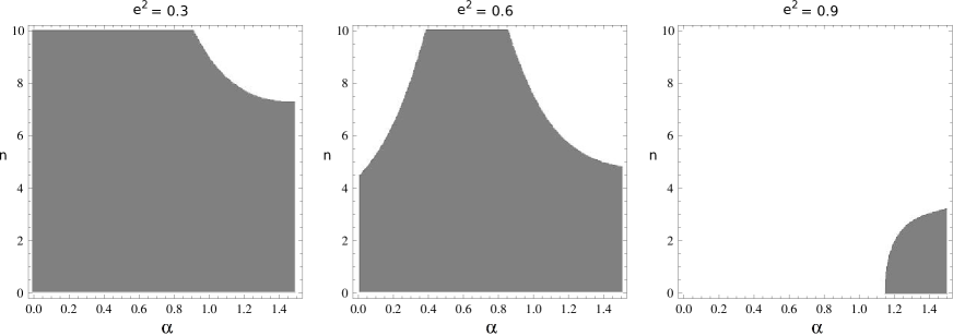
Figure 5: Sections of the parameter space of constant $e^{2}$, showing where the dynamical symmetry breaking occurs, using the improved effective potential.

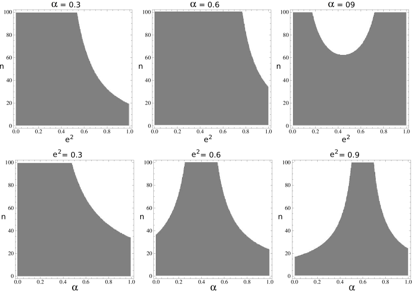
Figure 6: Sections of the parameter space of constant $e^{2}$ or $\alpha$, showing where the dynamical symmetry breaking occurs, using the unimproved 2-loop calculation of the effective potential.

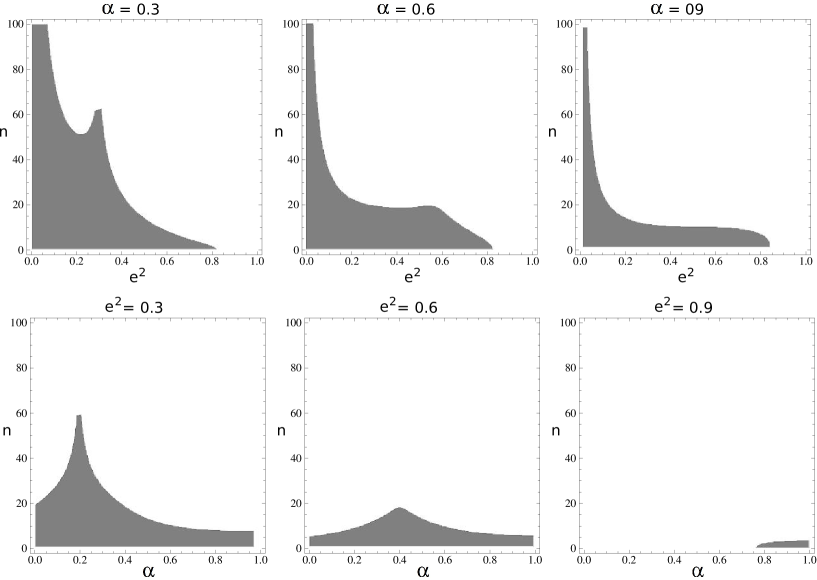
Figure 7: Same as Fig. 6, but using the improved effective potential. It is apparent that when $e^{2}=\alpha$, the effective potential is stable for higher values of $n$; this feature can also be seen in Fig. 6.

Another interesting fact is that, for certain values of $x$, $z$, and $n$, Eq. (107) provides two viable solutions for $y$. This is true both for the unimproved as well as for the improved effective potential. For example, for $e^{2}=0.5$, $\alpha=0.5$ and $n=1$, the unimproved potential leads to the equation

$$-200.852y^{2}+60.376y-0.0120817=0\,,$$ (108)

for the determination of $y$, from which we obtain two solutions

$$y_{1} =0.30039\,,$$ (109a)

$$y_{2} =0.00020\,.$$ (109b)

The corresponding masses predicted for the scalar are $m_{1}=7.7907\mu^{2}$ and $m_{2}=0.00519\mu^{2}$. For the same value values of the parameters $e^{2}$, $\alpha$ and $n$, the improved effective potential yields

$$-4.75607\times 10^{9}y^{7}-4.75649\times 10^{8}y^{6}-2.46246\times 10^{7}y^{5}-882982.y^{4}$$

$$-24137.9y^{3}-471.335y^{2}+60.0824y-0.0379559 =0\,,$$ (110)

whose positive and real solutions are

$$y_{1} =0.02540\,,$$ (111a)

$$y_{2} =0.00063\,,$$ (111b)

providing $m_{1}=0.18595\mu^{2}$ and $m_{1}=0.015843\mu^{2}$.

Figure 8 depicts the region of the $\alpha-e^{2}$ plane, for $n=5$, where such a duplicity of solutions occurs, both for the unimproved and improved effective potentials. The most important difference between the two cases is that the improved effective potential drastically reduces the range of parameters where the duplicity happens. Figure 9 shows how the situation changes for different values of $n$, for the second case.

The pattern in Eqs. (110,111) is quite typical: the solution $y_{2}$ is smaller than $y_{1}$. Fixing the parameters $e^{2}=0.5$ and $n=1$, $y_{2}$ becomes smaller as $\alpha$ increases. At some point, the solution $y_{1}$ approaches zero and becomes negative, so it is not counted anymore as a viable solution. This behavior is clearly visible at the first graph in Fig. 10. For fixed $\alpha$ and $n$, the situation is reversed: $y_{2}$ becomes smaller as $\alpha$ decreases, as also seen in Fig. 10.

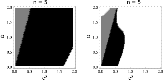
Figure 8: Regions of the $e^{2}$-$\alpha$ plane, for $n=1$, painted according to the number of viable solutions $y$ for Eq. (107) for the unimproved effective potential (left) and for the improved one (right). Black, gray and white means two, one, and none solutions, respectively.

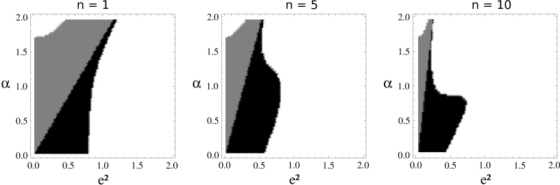
Figure 9: Same as Fig. 8 (right), but for different values of $n$. For larger $n$, the region where we found a unique solution for the conformal symmetry breaking becomes smaller in absolute terms, and also in comparison to the region where we found two solutions.

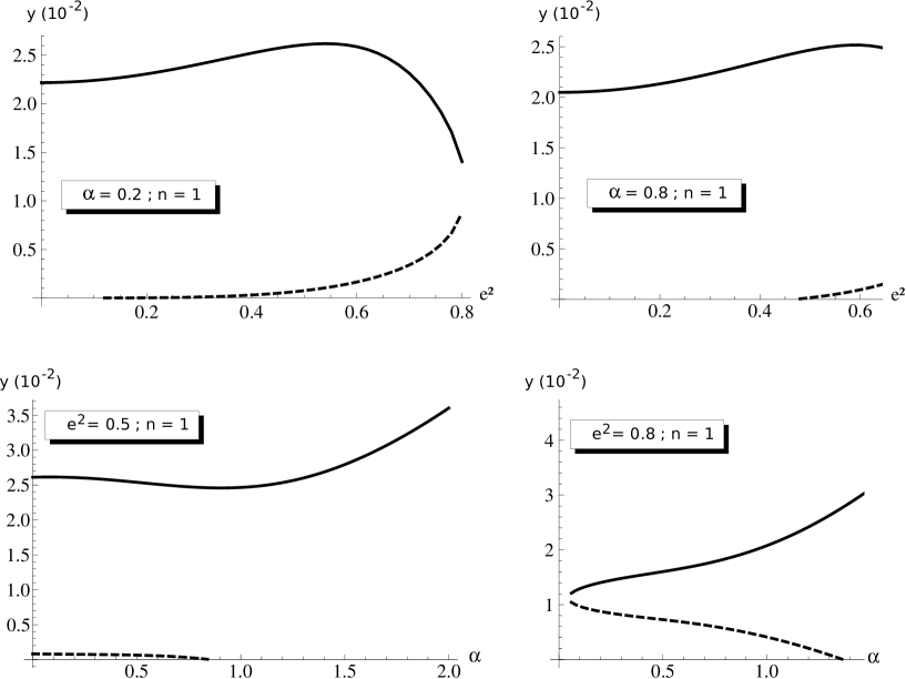
Figure 10: Behavior of the two solutions $y_{1}$ and $y_{2}$ (solid and dashed lines, respectively) when varying the parameters of the model.

In summary, there are regions of the parameter space of the theory where there are two possible vacua, in which the conformal symmetry was broken by radiative corrections. The scalar selfcoupling and mass are clearly different for these two vacua. Our numerical studies show, however, that for the improved effective potential, the region of the parameter space where such a situations takes place is much smaller than for the unimproved potential.

VII Conclusions

The Renormalization Group Equation is well known to provide better approximations to the effective potential of a given model than a pure perturbative calculation up to a given loop order. In this work, we pursued the idea of using the RGE to sum infinite subseries of the expansion of the effective potential in powers of coupling constants and logarithms $L=\ln\left(\phi^{2}/\mu\right)$.

We focused on a Chern-Simons theory coupled to a fermion and a complex scalar field. Renormalization group beta-functions and anomalous dimensions should be known up to the two-loop order; we collected results already available in the literature and calculated the beta-function for the Yukawa coupling and the wavefunction renormalization of the fermionic field. With this information, we were able to use the RGE to extract the maximum amount of information of the perturbative calculation, obtaining and improved effective potential which, in principle, should allows us to establish more precisely the properties of the model. In particular, we were interested in studying the phase where the conformal symmetry breaking of the model is broken by the radiative corrections.

By comparing the outcomes of the standard analysis of dynamical symmetry breaking in the model using the standard effective action calculated from loop corrections and the improved one, we shown how the latter indeed provides a more precise determination of the properties of the model in the broken phase. This should serve as an instructive example of the relevance of using the RGE to obtain the maximum amount of information on the effective action from a given perturbative calculation. This idea is quite relevant in the context of models with classical conformal invariance which is broken at the quantum level, for the sake of obtaining the most precise predictions.

It would be interesting to extend the calculations discussed in this work to higher loop orders, to see whether this would imply in some mild refinement of the results presented here, or some even more drastic reduction of the parameter space region where the dynamical symmetry breaking happens.

Acknowledgments. The authors thank M. Gomes for reading the manuscript. This work was partially supported by the Brazilian agencies Conselho Nacional de Desenvolvimento Científico e Tecnológico (CNPq) and Fundação de Amparo à Pesquisa do Estado de São Paulo (FAPESP).

References

(1)S. Deser, R. Jackiw and S. Templeton,
Ann. Phys. 140, 372 (1982).
(2)W. Chen, G.W. Semenoff, and Y.S. Wu, Phys.
Rev. D 46, 5521 (1992).
(3)S. Coleman and E. Weinberg, Phys. Rev. D 7,
1888 (1973).
(4)V. Elias, R. B. Mann, D. G. C. McKeon and T. G.
Steele, Phys. Rev. Lett. 91, 251601 (2003); V. Elias, R.
B. Mann, D. G. C. McKeon and T. G. Steele, Nucl. Phys. B 678,
147 (2004) [Erratum-ibid.B 703, 413 (2004)]; F. A. Chishtie,
V. Elias, R. B. Mann, D. G. C. McKeon and T. G. Steele, Nucl. Phys.
B 743, 104 (2006).
(5)V. Elias, D. G. C. McKeon and T. G. Steele,
Int. J. Mod. Phys. A 18, 3417 (2003); F. A. Chishtie, V.
Elias, R. B. Mann, D. G. C. McKeon and T. G. Steele, Int. J. Mod.
Phys. E 16, 1681 (2007); V. Elias, D. G. C. McKeon and T.
N. Sherry, Int. J. Mod. Phys. A 20, 1065 (2005).
(6)K. A. Meissner and H. Nicolai, Eur. Phys. J. C
57, 493 (2008).
(7)K. A. Meissner and H. Nicolai, Acta Phys. Polon.
B 40, 2737 (2009).
(8)A. G. Dias, Phys. Rev. D 73, 096002 (2006).
(9)P-N. Tan, B. Tekin, and Y. Hosotani, Nucl. Phys.
B 502, 483 (1997).
(10)L. V. Avdeev, G. V. Grigoryev, and D. I. Kazakov,
Nucl. Phys. B 382, 561 (1992).
(11)V. S. Alves, M. Gomes, S. L. V. Pinheiro, and
A. J. da Silva, Phys. Rev. D 61, 065003 (2000).
(12)A. G. Dias, M. Gomes and A. J. da Silva, Phys. Rev.
D 69, 065011 (2004).
(13)W. Siegel, Phys. Lett. B 84, 193 (1979).
(14)K. A. Meissner and H. Nicolai, Phys. Lett.
B 648, 312 (2007).
(15)A. G. Dias, M.Sc. thesis, Instituto de Física
da Universidade de São Paulo, 2002.