Systematics of the magnetic-Prandtl-number dependence of homogeneous, isotropic magnetohydrodynamic turbulence

Abstract

We present the results of our detailed pseudospectral direct numerical simulation (DNS) studies, with up to $1024^{3}$ collocation points, of incompressible, magnetohydrodynamic (MHD) turbulence in three dimensions, without a mean magnetic field. Our study concentrates on the dependence of various statistical properties of both decaying and statistically steady MHD turbulence on the magnetic Prandtl number ${\rm Pr_{M}}$ over a large range, namely, $0.01\leq{\rm Pr_{M}}\leq 10$. We obtain data for a wide variety of statistical measures such as probability distribution functions (PDFs) of moduli of the vorticity and current density, the energy dissipation rates, and velocity and magnetic-field increments, energy and other spectra, velocity and magnetic-field structure functions, which we use to characterise intermittency, isosurfaces of quantities such as the moduli of the vorticity and current, and joint PDFs such as those of fluid and magnetic dissipation rates. Our systematic study uncovers interesting results that have not been noted hitherto. In particular, we find a crossover from larger intermittency in the magnetic field than in the velocity field, at large ${\rm Pr_{M}}$, to smaller intermittency in the magnetic field than in the velocity field, at low ${\rm Pr_{M}}$. Furthermore, a comparison of our results for decaying MHD turbulence and its forced, statistically steady analogue suggests that we have strong universality in the sense that, for a fixed value of ${\rm Pr_{M}}$, multiscaling exponent ratios agree, at least within our errorbars, for both decaying and statistically steady homogeneous, isotropic MHD turbulence.

1 Introduction

The hydrodynamics of conducting fluids is of great importance in many terrestrial and astrophysical phenomena. Examples include the generation of magnetic fields via dynamo action in the interstellar medium, stars, and planets [1, 2, 3, 4, 5, 6, 7, 8, 9, 10, 11], and liquid-metal systems [12, 13, 14, 15, 16, 17, 18] that are studied in laboratories. The flows in such settings, which can be described at the simplest level by the equations of magnetohydrodynamics (MHD), are often turbulent [5]. The larger the kinetic and magnetic Reynolds numbers, ${\rm Re}=UL/\nu$ and ${\rm Re_{M}}=UL/\eta$, respectively, the more turbulent is the motion of the conducting fluid; here $L$ and $U$ are typical length and velocity scales in the flow, $\nu$ is the kinematic viscosity, and $\eta$ is the magnetic diffusivity. The statistical characterization of turbulent MHD flows, which continues to pose challenges for experiments [19], direct numerical simulations [20], and theory [21], is even harder than its analogue in fluid turbulence because (a) we must control both ${\rm Re}$ and ${\rm Re_{M}}$ and (b) we must obtain the statistical properties of both velocity and magnetic fields.

The kinematic viscosity $\nu$ and the magnetic diffusivity $\eta$ can differ by several orders of magnitude, so the magnetic Prandtl number ${\rm Pr_{M}}\equiv{\rm Re_{M}}/{\rm Re}=\nu/\eta$ can vary over a large range. For example, ${\rm Pr_{M}}\simeq 10^{-5}$ in the liquid-sodium system [15, 16], ${\rm Pr_{M}}\simeq 10^{-2}$ at the base of the Sun’s convection zone [22], and ${\rm Pr_{M}}\simeq 10^{14}$ in the interstellar medium [8, 20]. Furthermore, two dissipative scales play an important role in MHD; they are the Kolmogorov scale $\ell_{d}$ ($\sim\nu^{3/4}$ at the level of Kolmogorov 1941 (K41) phenomenology [23, 24]) and the magnetic-resistive scale $\ell_{d}^{M}$ ($\sim\eta^{3/4}$ in K41). A thorough study of the statistical properties of MHD turbulence must resolve both these dissipative scales. Given current computational resources, this is a daunting task at large ${\rm Re}$ especially if ${\rm Pr_{M}}$ is significantly different from unity. Thus, most direct numerical simulations (DNS) of MHD turbulence [25, 26, 27, 28, 29, 30] have been restricted to ${\rm Pr_{M}}\simeq 1$. Some DNS studies have now started moving away from the ${\rm Pr_{M}}\simeq 1$ regime especially in the context of the dynamo problem [31, 32].

Here we initiate a detailed DNS study of the statistical properties of incompressible, homogeneous, and isotropic MHD turbulence for a large range of the magnetic Prandtl number, namely, $0.01\leq{\rm Pr_{M}}\leq 10$. There is no mean magnetic field in our DNS [33]; and we restrict ourselves to Eulerian measurements [34]. Before we give the details of our DNS study, we highlight a few of our qualitative, principal results. Elements of some of our results, for the case ${\rm Pr_{M}}=1$ and for quantities such as energy spectra, exist in the MHD-turbulence literature as can be seen from the representative Refs. [5, 6, 25, 35, 36, 37, 38]. However, to the best of our knowledge, no study has attempted as detailed and systematic an investigation of the statistical properties of MHD turbulence as we present here, especially with a view to elucidating their dependence on ${\rm Pr_{M}}$. Our study uncovers interesting trends that have not been noted hitherto. These emerge from our detailed characterisation of intermittency, via a variety of measures which include various probability distribution functions (PDFs) such as those of the modulus of the vorticity and the energy dissipation rates, velocity and magnetic-field structure functions that can be used to characterise intermittency, isosurfaces of quantities such as the moduli of the vorticity and current, and joint PDFs such as those of fluid and magnetic dissipation rates. Earlier DNS studies [30] have suggested that intermittency, as characterised say by the multiscaling exponents for velocity- and magentic-field structure functions, is more intense for the magnetic field than for the velocity field when ${\rm Pr_{M}}=1$. Our study confirms this and suggests, in addition, that this result is reversed as we lower ${\rm Pr_{M}}$. This crossover from larger intermittency in the magnetic field than in the velocity field, at large ${\rm Pr_{M}}$, to smaller intermittency in the magnetic field than in the velocity field, at low ${\rm Pr_{M}}$, shows up not only in the values of multiscaling exponent ratios, which we obtain from a detailed local-slope analysis of extended-self-similarity (ESS) plots [39, 40] of one structure function against another, but also in the behaviours of tails of PDFs of dissipation rates, the moduli of vorticity and current density, and velocity and magnetic-field increments. Furthermore, a comparison of our results for decaying MHD turbulence and its forced, statistically steady analogue suggest that, at least given our conservative errors, the homogeneous, isotropic MHD turbulence that we study here displays strong universality [41, 42] in the sense that multiscaling exponent ratios agree for both decaying and statistically steady cases.

The remaining part of this paper is organised as follows. In Sec. 2 we describe the MHD equations, the details of the numerical schemes we use (Subsection 2.1), and the statistical measures we use to characterise MHD turbulence (Subsection 2.2). In Sec. 3 we present our results; these are described in the seven Subsections 3.1, 3.2, 3.3, 3.4, 3.5, 3.6, and 3.7 that are devoted, respectively, to (a) a summary of well-known results from fluid turbulence that are relevant to our study, (b) the temporal evolution of quantities such as the energy and energy-dissipation rates, (c) energy, dissipation-rate, Elsässer-variable, and effective-pressure spectra, (d) various probability distribution functions (PDFs) that can be used, inter alia, to characterise the alignments of vectors such as the vorticity with, say, the eigenvectors of the rate-of-strain tensor, (e) velocity and magnetic-field structure functions that can be used to characterise intermittency, (f) isosurfaces of quantities such as the moduli of the vorticity and current, and (g) and joint PDFs such as those of fluid and magnetic dissipation rates. Section 4 contains a discussion of our results.

2 MHD Equations

The hydrodynamics of a conducting fluid is governed by the MHD equations [1, 2, 3, 4, 5, 7], in which the Navier-Stokes equation for a fluid is coupled to the induction equation for the magnetic field:

$$\frac{\partial{\bf u}}{\partial t}+({\bf u}\cdot\nabla){\bf u}=\nu\nabla^{2}{\bf u}-\nabla\bar{p}+({\bf b}\cdot\nabla){\bf b}+{\bm{f}}_{u},$$ (1)

$$\frac{\partial{\bf b}}{\partial t}+({\bf u}\cdot\nabla){\bf b}=({\bf b}\cdot\nabla){\bf u}+\eta\nabla^{2}{\bf b}+{\bm{f}}_{b};$$ (2)

here ${\bf u}$, ${\bf b}$, ${\bm{\omega}}=\nabla\times{\bf u}$ and ${\bf j}=\nabla\times{\bf b}$ are, respectively, the velocity field, the magnetic field, the vorticity, and the current density at the point $\bf{x}$ and time $t$; $\nu$ and $\eta$ are the kinematic viscosity and the magnetic diffusivity, respectively, and the effective pressure is $\bar{p}=p+(b^{2}/8\pi)$, where $p$ is the pressure; ${\bm{f}}_{u}$ and ${\bm{f}}_{b}$ are the external forces; while studying decaying MHD turbulence we set ${\bm{f}}_{u}={\bm{f}}_{b}=0$. The MHD equations can also be written in terms of the Elsässer variables ${\bf z}^{\pm}={\bf u}\pm{\bf b}$ [7, 25]. We restrict ourselves to low-Mach-number flows so we use the incompressibility condition $\nabla\cdot{\bf u}({\bf x},t)=0$; and we must, of course, impose $\nabla\cdot{\bf b}({\bf x},t)=0$. By using the incompressibility condition, we can eliminate the effective pressure and obtain the velocity and magnetic fields via a pseudospectral method that we describe in the next Subsection. The effective pressure then follows from the solution of the Poisson equation

$$\nabla^{2}{\bar{p}}=\nabla\cdot[({\bf b}\cdot\nabla){\bf b}-({\bf u}\cdot\nabla){\bf u}].$$ (3)

2.1 Direct Numerical Simulation

Table 1: List of parameters for our 16 DNS runs R1-R5, R3B-R5B, R1C-R4C, and R1D-R4D: $N^{3}$ is the number of collocation points in our simulation, $\nu$ is the kinematic viscosity, ${\rm Pr_{M}}$ is magnetic Prandtl number, $\delta t$ is time step; $u_{\rm rms}$, $\lambda$, and ${\rm Re}_{\lambda}$ are the root-mean-sqare velocity, the Taylor microscale, and the Taylor-microscale Reynolds number, respectively. These are obtained at $t_{c}$ for our decaying-MHD-turbulence runs R1-R5, R3B-R5B, and R1C-R4C; and for statistically steady MHD turbulence (runs R1D-R4D) these are averaged over the statistically steady state; here $t_{c}$ (iteration steps multiplied by $\delta t$) is the time at which the cascades for both the fluid and magnetic fields are completed (see text); $\eta_{d}^{u}$ and $\eta_{d}^{b}$ are, respectively, the Kolmogorov dissipation length scales for the fluid and magnetic fields. $k_{\rm max}$ is the magnitude of the largest-magnitude wave vectors resolved in our DNS studies which use the $2/3$ dealiasing rule; $k_{\rm max}\simeq 170.67$ and $341.33$ for $N=512$ and $1024$, respectively.

Runs	$N$	$\nu$	${\rm Pr_{M}}$	$\delta t$	$u_{\rm rms}$	$\lambda$	${\rm Re}_{\lambda}$	$t_{c}$	$k_{\rm max}\eta_{d}^{u}$	$k_{\rm max}\eta_{d}^{b}$
R1	$512$	$10^{-4}$	$0.1$	$10^{-3}$	$0.34$	$0.18$	$610$	$9.7$	$0.629$	$2.280$
R2	$512$	$5\times 10^{-4}$	$0.5$	$10^{-3}$	$0.34$	$0.27$	$187$	$9.1$	$1.752$	$2.389$
R3	$512$	$10^{-3}$	$1$	$10^{-3}$	$0.34$	$0.35$	$121$	$8.1$	$2.772$	$2.444$
R4	$512$	$5\times 10^{-3}$	$5$	$10^{-3}$	$0.33$	$0.60$	$39$	$7.0$	$8.224$	$2.692$
R5	$512$	$10^{-2}$	$10$	$10^{-3}$	$0.31$	$0.73$	$23$	$6.5$	$13.267$	$2.836$
R3B	$512$	$10^{-3}$	$1$	$10^{-4}$	$1.07$	$0.20$	$210$	$3.1$	$1.175$	$1.052$
R4B	$512$	$5\times 10^{-3}$	$5$	$10^{-4}$	$2.32$	$0.24$	$110$	$1.4$	$1.961$	$0.644$
R5B	$512$	$10^{-2}$	$10$	$10^{-4}$	$3.21$	$0.26$	$85$	$1.0$	$2.490$	$0.520$
R1C	$1024$	$10^{-4}$	$0.01$	$10^{-4}$	$0.35$	$0.23$	$810$	$8.0$	$1.431$	$22.12$
R2C	$1024$	$10^{-4}$	$0.1$	$10^{-4}$	$1.11$	$0.08$	$890$	$2.9$	$0.472$	$1.690$
R3C	$1024$	$10^{-3}$	$1$	$10^{-4}$	$1.14$	$0.15$	$172$	$2.5$	$1.996$	$1.779$
R4C	$1024$	$10^{-2}$	$10$	$10^{-4}$	$2.37$	$0.24$	$57$	$1.1$	$5.550$	$1.164$
R1D	$512$	$10^{-4}$	$0.01$	$10^{-4}$	$1.31$	$0.18$	$2367$	$--$	$0.320$	$5.364$
R2D	$512$	$10^{-4}$	$0.1$	$10^{-4}$	$0.99$	$0.14$	$1457$	$--$	$0.334$	$1.145$
R3D	$512$	$10^{-3}$	$1$	$10^{-4}$	$1.06$	$0.17$	$239$	$--$	$1.264$	$1.033$
R4D	$512$	$10^{-2}$	$10$	$10^{-4}$	$1.04$	$0.23$	$61$	$--$	$6.505$	$1.129$

Our goal is to study the statistical properties of homogeneous and isotropic MHD turbulence so we use periodic boundary conditions and a standard pseudospectral method [43] with $N^{3}$ collocation points in a cubical simulation domain with sides of length $L=2\pi$; thus, we evaluate spatial derivatives in Fourier space and local products of fields in real space. We use the $2/3$ dealiasing method [43] to remove aliasing errors; after this dealiasing $k_{\rm max}$ is the magnitude of the largest-magnitude wave vectors resolved in our DNS studies. We have carried out extensive simulations with $N=512$ and $N=1024$; the parameters that we use for different runs are given in Table 1 for decaying and statistically steady turbulence.

We use a second-order, slaved, Adams-Bashforth scheme, with a time step $\delta t$, for the time evolution of the velocity and magnetic fields; this time step is chosen such that the Courant-Friedrichs-Lewy (CFL) condition is satisfied [44].

In our decaying-MHD-turbulence studies we have taken the initial (superscript $0$) energy spectra $E_{u}^{0}(k)$ and $E_{b}^{0}(k)$, for velocity and magnetic fields, respectively, to be the same; specifically, we have chosen

$$E_{u}^{0}(k)=E_{b}^{0}(k)=E^{0}k^{4}\exp(-2k^{2}),$$ (4)

where $E^{0}$, the initial amplitude, is chosen in such a way that we resolve both fluid and magnetic dissipation scales $\eta^{u}_{d}$ and $\eta^{b}_{d}$, respectively: in all, except a few, of our runs $k_{\rm max}\eta^{u}_{d}\gtrsim 1$ and $k_{\rm max}\eta^{b}_{d}\gtrsim 1$. The initial phases of the Fourier components of the velocity and magnetic fields are taken to be different and chosen such that they are distributed randomly and uniformly between $0$ and $2\pi$. In such studies, it is convenient to pick a reference time at which various statistical properties can be compared. One such reference time is the peak that occurs in a plot of the energy dissipation versus time; this reference time has been used in studies of decaying fluid turbulence [45, 46], decaying fluid turbulence with polymer additives [47, 48], and decaying MHD turbulence [25, 26, 49]. Such peaks are associated with the completion of the energy cascade from large length scales, at which energy is injected into the system, to small length scales at which viscous losses are significant. In the MHD case, these peaks occur at slightly different times, $t_{u}$ and $t_{b}$, respectively, in plots of the kinetic ($\epsilon_{u}$) and magnetic ($\epsilon_{b}$) energy-dissipation rates. In our decaying-MHD-turbulence studies we store velocity and magnetic fields at the time $t_{c}$; if $t_{u}>t_{b}$, $t_{c}=t_{u}$; and $t_{c}=t_{b}$ otherwise; from these fields we calculate the statistical properties that we present in the next Section.

In the simulations in which we force the MHD equations to obtain a nonequilibrium statistically steady state (NESS), we use a generalization of the constant-energy-injection method described in Ref. [50]. We do not force the magnetic field directly so we choose ${\bm{f}}_{b}=0$. The force ${\bm{f}}_{u}({\bf x},t)$ is specified most simply in terms of ${\tilde{\bm{f}}}_{u}({\bf k},t)$, its spatial Fourier components, as follows:

$${\tilde{\bm{f}}}_{u}({\bf k},t)=\frac{{\mathcal{P}}~{}\Theta(k_{f}-k)}{2E_{u}(k_{f},t)}{\tilde{\bf u}}({\bf k},t),$$ (5)

where $\Theta(k_{f}-k)$ is $1$ if $k\leq k_{f}$ and $0$ otherwise, ${\mathcal{P}}$ is the power input, and $E_{u}(k_{f},t)=\sum_{k\leq k_{f}}E_{u}({\bf k},t)$; in our DNS we use $k_{f}=2$. This yields a statistically steady state in which the mean value of the total energy dissipation rate per unit volume balances the power input, i.e.,

$$\langle\epsilon\rangle={\mathcal{P}};$$ (6)

once this state has been established, we save 50 representative velocity- and magnetic-field configurations over $\simeq 36.08t_{I}$, $29.29t_{I}$, $32.61t_{I}$, and $30.95t_{I}$, for R1D, R2D, R3D, and R4D, respectively, where $t_{I}=\ell_{I}/u_{\rm rms}$ is the integral-scale eddy-turnover time. We use these configurations to obtain the statistical properties that we describe below.

For decaying MHD turbulence we have carried out eight simulations with $512^{3}$ collocation points and four simulations with $1024^{3}$ collocation points. The parameters used in these simulations, which we have organised into three sets, are given in Table 1.

In the first set of runs, R1-R5, we set the magnetic diffusivity $\eta=10^{-3}$ and use five values of $\nu$, namely, $10^{-4},\,5.0\times 10^{-4},\,10^{-3},\,5.0\times 10^{-3},$ and $10^{-2}$, which yield ${\rm Pr_{M}}=0.1,\,0.5,\,1,\,5$, and $10$. These runs have been designed to study the effects, on decaying MHD turbulence, of an increase in ${\rm Pr_{M}}$, with the initial energy held fixed: in particular, we use $E^{0}_{u}=E^{0}_{b}\simeq 0.32$ in Eq. 4 for runs R1-R5. Given that this initial energy and $\eta$ are both fixed, an increase in ${\rm Pr_{M}}$ leads to a decrease in ${\rm Re}$, and thus an increase in $k_{\rm max}\eta^{u}_{d}$ and $k_{\rm max}\eta^{b}_{d}$ as we discuss in detail later.

In our second set of decaying-MHD-turbulence runs, R3B, R4B and R5B, we increase $E^{0}$ in Eq. 4 as we increase $\nu$, and thereby ${\rm Pr_{M}}$, so that $k_{\rm max}\eta^{u}_{d}\simeq 1$ and $k_{\rm max}\eta^{b}_{d}\simeq 1$. Thus, in these runs, the inertial ranges in energy spectra extend over comparable ranges of the wave-vector magnitude $k$.

Our third set of decaying-MHD-turbulence runs, R1C, R2C, R3C, and R4C, use $1024^{3}$ collocation points and ${\rm Pr_{M}}=0.01,\,0.1,\,1$, and $10$, respectively. By comparing the results of these runs with those of R1-R5, R3B, R4B, and R5B, we can check whether our qualitative results depend significantly on the number of collocation points that we use.

We have carried out another set of four runs, R1D, R2D, R3D, and R4D, in which we force the MHD equations, as described above, until we obtain a nonequilibrium statistically steady state. These runs help us to compare the statistical properties of decaying and statistically steady turbulence. In these runs we use $512^{3}$ collocation points, and $\nu$ and $\eta$ such that ${\rm Pr_{M}}=0.01,~{}0.1,~{}1$, and $10$, respectively.

2.2 Statistical measures

We use several statistical measures to characterise homogeneous, isotropic MHD turbulence. Some, but not all, of these have been used in earlier DNS studies [25, 29, 35, 37, 51, 52, 53] and solar-wind turbulence [54, 55, 56].

We calculate the kinetic, magnetic, and total energy spectra $E_{u}(k)=\sum_{{\bf k}\ni|{\bf k}|=k}|{\tilde{\bf u}}({\bf k})|^{2}$, $E_{b}(k)=\sum_{{\bf k}\ni|{\bf k}|=k}|{\tilde{\bf b}}({\bf k})|^{2}$, and $E(k)=E_{u}(k)+E_{b}(k)$, respectively, the kinetic, magnetic, and total energies $E_{u}=\sum_{k}E_{u}(k)/2$, $E_{b}=\sum_{k}E_{b}(k)/2$, and $E=E_{u}+E_{b}$, and the ratio $E_{b}/E_{u}$. Spectra for the Elsässer variables, energy dissipation rates, and the effective pressure are, respectively, $E_{z^{\pm}}(k)=\sum_{{\bf k}\ni|{\bf k}|=k}|{\tilde{\bf z}^{\pm}}({\bf k})|^{2}$, $\epsilon_{u}(k)=\nu k^{2}E_{u}(k)$, $\epsilon_{b}(k)=\nu k^{2}E_{b}(k)$, and $P(k)=\sum_{{\bf k}\ni|{\bf k}|=k}|\tilde{\bar{p}}({\bf k})|^{2}$.

Our MHD simulations are characterised by the Taylor-microscale Reynolds number ${\rm Re}_{\lambda}=u_{\rm rms}\lambda/\nu$, the magnetic Taylor-microscale Reynolds number ${\rm Rm}_{\lambda}=u_{\rm rms}\lambda/\eta$, and the magnetic Prandtl number ${\rm Pr_{M}}={\rm Rm}_{\lambda}/{\rm Re}_{\lambda}=\nu/\eta$, where the root-mean-square velocity $u_{\rm rms}=\sqrt{2E_{u}/3}$ and the Taylor microscale $\lambda=\left[\sum_{k}k^{2}E(k)/E\right]^{-1/2}$. We also calculate the integral length scale $\ell_{I}=\left[\sum_{k}E(k)/k\right]/E$, the mean kinetic energy dissipation rate per unit mass, $\epsilon_{u}=\nu\sum_{i,j}(\partial_{i}u_{j}+\partial_{j}u_{i})^{2}=\nu\sum_{k}k^{2}E_{u}(k)$, the mean magnetic energy dissipation rate per unit mass $\epsilon_{b}=\eta\sum_{i,j}(\partial_{i}b_{j}+\partial_{j}b_{i})^{2}=\eta\sum_{k}k^{2}E_{b}(k)$, the mean energy dissipation rate per unit mass $\epsilon=\epsilon_{u}+\epsilon_{b}$, and the dissipation length scales for velocity and magnetic fields $\eta_{d}^{u}=(\nu^{3}/\epsilon_{u})^{1/4}$ and $\eta_{d}^{b}=(\eta^{3}/\epsilon_{b})^{1/4}$, respectively.

We calculate the eigenvalues $\Lambda_{n}^{u}$ and the associated eigenvectors ${\hat{e}}_{n}^{u}$, with $n=1,2,$ or $3$, of the rate-of-strain tensor $\mathbb{S}$ whose components are $S_{ij}=\partial_{i}u_{j}+\partial_{j}u_{i}$. Similarly $\Lambda_{1}^{b}$, $\Lambda_{2}^{b}$ and $\Lambda_{3}^{b}$ denote the eigenvalues of the tensile magnetic stress tensor $\mathbb{T}$, which has components $T_{ij}=-b_{i}b_{j}$; the corresponding eigenvectors are, respectively, ${\hat{e}}_{1}^{b}$, ${\hat{e}}_{2}^{b}$, and ${\hat{e}}_{3}^{b}$.

For incompressible flows $\sum_{n}\Lambda_{n}^{u}=0$, so at least one of the eigenvalues $\Lambda_{n}^{u}$ must be positive and another negative; we label them in such a way that $\Lambda_{3}^{u}$ is positive, $\Lambda_{1}^{u}$ negative, and $\Lambda_{2}^{u}$ lies in between them; note that $\Lambda_{2}^{u}$ can be positive or negative. We obtain probability distribution functions (PDFs) of these eigenvalues; furthermore, we obtain PDFs of the cosines of the angles that the associated eigenvectors make with the vectors such as ${\bf u}$, ${\bm{\omega}}$, etc. These PDFs and those of quantities such as the local cross helicity $H_{C}={\bf u}\cdot{\bf b}$ help us to quantify the degree of alignment of pairs of vectors such as ${\bf u}$ and ${\bf b}$ [52]. We also compare PDFs of magnitudes of local vorticity $\omega$, the current density $j$, and local energy dissipation rates $\epsilon_{u}$ and $\epsilon_{b}$ to get information about intermittency in velocity and magnetic fields.

We also obtain several interesting joint PDFs; to the best of our knowledge, these have not been obtained earlier for MHD turbulence. We first obtain the velocity-derivative tensor $\mathbb{A}$, also known as the rate-of-deformation tensor, with components $A_{ij}=\partial_{i}u_{j}$, and thence the invariants $Q=-\frac{1}{2}tr(\mathbb{A}^{2})$ and $R=-\frac{1}{3}tr(\mathbb{A}^{3})$, which have been used frequently to characterise fluid turbulence [57, 58, 59]. The zero-discriminant line $D\equiv\frac{27}{4}R^{2}+Q^{3}=0$ and the $Q$ and $R$ axes divide the $QR$ plane into qualitatively different regimes. In particular, regions in a turbulent flow can be classified as follows: when $Q$ is large and negative, local strains are high and vortex formation is not favoured; furthermore, if $R>0$, fluid elements experience axial strain, whereas, if $R<0$, they feel biaxial strain. In contrast, when $Q$ is large and positive, vorticity dominates the flow; if, in addition, $R<0$, vortices are compressed, whereas, if $R>0$, they are stretched. Thus, some properties of a turbulent flow can be highlighted by making contour plots of the joint PDF of $Q$ and $R$; these $QR$ plots show a characteristic, tear-drop shape. We explore the forms of these and other joint PDFs, such as joint PDFs of $\epsilon_{u}$ and $\epsilon_{b}$, in MHD turbulence.

To characterise intermittency in MHD turbulence we calculate the order-$p$, equal-time, longitudinal structure functions $S_{p}^{a}(l)\equiv\langle|\delta a_{\parallel}({\bf x},l)|^{p}\rangle$, where the longitudinal component of the field ${\bf a}$ is given by $\delta a_{\parallel}({\bf x},l)\equiv[{\bf a}({\bf x}+{\bf l},t)-{\bf a}({\bf x},t)]\cdot\frac{{\bf l}}{l}$, where ${\bf a}$ can be ${\bf u}$, ${\bf b}$, or one of the Elsässer variables. From these structure functions we also obtain the hyperflatness $F_{6}^{a}(l)=S_{6}^{a}(l)/[S_{2}^{a}(l)]^{3}$. For separations $l$ in the inertial range, i.e., $\eta_{d}^{u},\eta_{d}^{b}\ll l\ll L$, we expect $S_{p}^{a}(l)\sim l^{\zeta_{p}^{a}}$, where $\zeta_{p}^{a}$ are the inertial-range multiscaling exponents for the field ${\bf a}$; the Kolmogorov phenomenology of 1941 [23, 24, 25], henceforth referred to as K41, yields the simple scaling result $\zeta_{p}^{aK41}=p/3$; but multiscaling corrections are significant with $\zeta_{p}^{a}\neq\zeta_{p}^{aK41}$ [Sec. 3]. From the increments $\delta a_{\parallel}({\bf x},l)\equiv[{\bf a}({\bf x}+{\bf l},t)-{\bf a}({\bf x},t)]\cdot\frac{{\bf l}}{l}$ we also obtain the dependence of PDFs of $\delta a_{\parallel}$ on the scale $l$.

3 Results

To set the stage for the types of studies we carry out for MHD turbulence, we begin with a very brief summary of similar and well-known results from studies of homogeneous, isotropic Navier-Stokes turbulence, which can be found, e.g., in Refs. [24, 45, 46, 60, 61, 62, 63, 64, 65, 66].

3.1 Overview of fluid turbulence

For ready reference we show here illustrative plots from a DNS study that we have carried out for the three-dimensional Navier-Stokes equation by using a pseudospectral method, with $512^{3}$ collocation points and the $2/3$ rule for removing aliasing errors; here $\nu=0.001$, ${\rm Re}_{\lambda}\simeq 340$ and $k_{\rm max}\eta_{d}^{u}\simeq 0.3$.

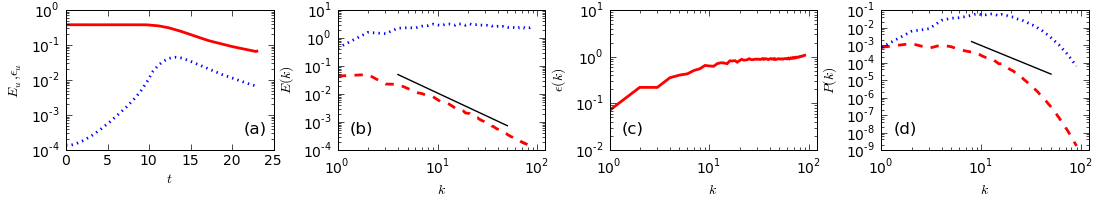
Figure 1: Plots from our DNS of decaying fluid turbulence in the Navier-Stokes equation with $512^{3}$ collocation points: (a) plots of the energy $E$ (red full line) and mean energy dissipation rate $\epsilon$ (blue dotted line) versus time $t$ (given as a product of the number of iterations and the time step $\delta t$); (b) log-log (base 10) plots of the energy spectrum $E(k)$ (red dashed line) and the corresponding compensated spectrum $k^{5/3}E(k)$ (blue dotted line) versus $k$. The black solid line shows the K41 result $k^{-5/3}$ for comparison; (c) log-log (base 10) plot of spectrum of energy-dissipation or enstrophy spectrum $\epsilon(k)$; (d) log-log (base 10) plots of the pressure spectrum $P(k)$ (red dashed line) and the compensated pressure spectrum $k^{7/3}P(k)$ (blue dotted line). The black solid line shows the K41 result $k^{-7/3}$ for comparison.

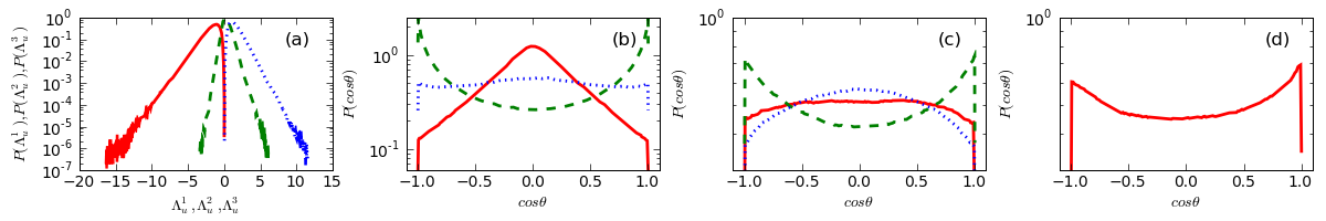
Figure 2: PDFs from our DNS of decaying fluid turbulence in Navier-Stokes equation with $512^{3}$ collocation points: (a) semilog (base 10) plots of PDFs of eigenvalues of rate-of-strain tensor ${\mathbb{S}}$, namely, $\Lambda_{1}^{u}$ (red full line), $\Lambda_{2}^{u}$ (green dashed line) and $\Lambda_{3}^{u}$ (blue dotted line); (b) semilog (base 10) plots of PDFs of cosines of angles between the vorticity ${\bm{\omega}}$ and eigenvectors of $\mathbb{S}$, namely, ${\hat{e}}_{1}^{u}$ (red full line), ${\hat{e}}_{2}^{u}$ (green dashed line), and ${\hat{e}}_{3}^{u}$ (blue dotted line); (c) semilog (base 10) plots of PDFs of cosines of angles between the velocity ${\bf u}$ and eigenvectors of $\mathbb{S}$, namely, ${\hat{e}}_{1}^{u}$ (red full line), ${\hat{e}}_{2}^{u}$ (green dashed line), and ${\hat{e}}_{3}^{u}$ (blue dotted line); (d) semilog (base 10) plots of PDFs of cosines of angles between the velocity ${\bf u}$ and vorticity ${\bm{\omega}}$.

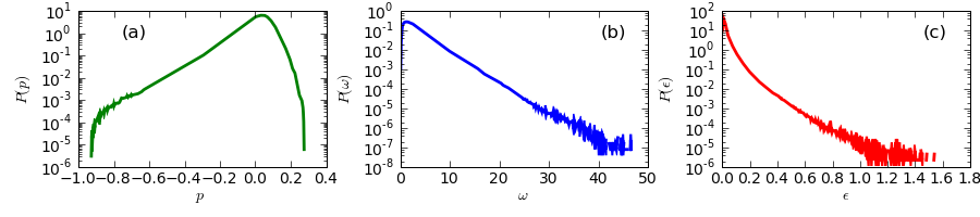
Figure 3: PDFs from our DNS of decaying fluid turbulence in Navier-Stokes equation with $512^{3}$ collocation points: semilog (base 10) plots of the PDFs of (a) the pressure $p$, (b) modulus of the vorticity $\omega$ and (c) the local energy-dissipation rate $\epsilon$.

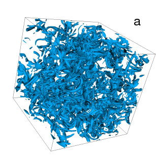
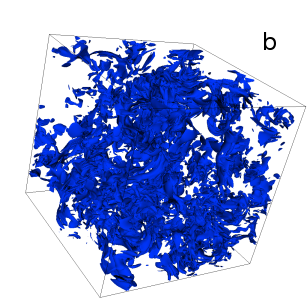
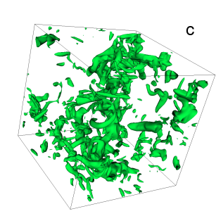
Figure 4: Isosurfaces of (a) the modulus of the vorticity $\omega$, (b) the local energy-dissipation rate $\epsilon$, and (c) the local pressure $p$, from our DNS of decaying fluid turbulence in Navier-Stokes equation with $512^{3}$ collocation points. The isovalues used in these plots are two standard deviations more than the mean values of the quantities.

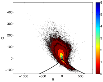
Figure 5: $QR$ plot, i.e., the joint PDF of $Q$ and $R$ (see text) shown as filled contour plot in our log-log (base 10) scale, obtained from a DNS of decaying fluid turbulence in Navier-Stokes equation with $512^{3}$ collocation points.

In decaying fluid turbulence, energy is injected at large spatial scales as described in the previous Section for the MHD case. This energy cascades down till it reaches the dissipative scale at which viscous losses are significant. We study various statistical properties; these are given in points (i)-(vi) below:

(i) Plots of the energy $E$ and the mean energy dissipation rate $\epsilon$ versus time show, respectively, a gentle decay and a maximum as shown, e.g., by the full red and dotted blue curves in Fig. 1(a). This maximum in $\epsilon$ is associated with the completion of the energy cascade at a time $t_{c}$; the remaining properties (ii)-(vi) are obtained at $t_{c}$. (ii) If ${\rm Re}_{\lambda}$ is sufficiently large and we have a well-resolved DNS (i.e., $k_{\rm max}\eta_{d}^{u}>1$), then, at $t_{c}$, the spectrum $E(k)$ shows a well-developed inertial range, where at the K41 level $E(k)\sim k^{-5/3}$, and a dissipation range, in which the behaviour of the energy spectrum is consistent with $E(k)\sim k^{\alpha}\exp(-\beta k)$, where $\alpha$ and $\beta$ are non-universal, positive constants [61, 64] and $5k_{d}<k<10k_{d}$, with $k_{d}=1/\eta_{d}^{u}$. An illustrative energy spectrum is shown by the dashed red line in Fig. 1(b); the blue dotted curve shows the compensated spectrum $k^{5/3}E(k)$; the associated dissipation or enstrophy spectrum $\epsilon(k)$ is shown in Fig. 1(c) and the inertial-range pressure spectrum [67], $P(k)\sim k^{-7/3}$ at the K41 level is shown in Fig. 1(d). [Note that our DNS for the Navier-Stokes equation, which suffices for our purposes of illustration, does not have a well-resolved dissipation range because $k_{\rm max}\eta_{d}^{u}\simeq 0.3<1$; this is also reflected in the lack of a well-developed maximum in the enstrophy spectrum of Fig. 1(c).] (iii) Illustrative PDFs of the eigenvalues $\Lambda_{n}^{u}$ of the rate-of-strain tensor $\mathbb{S}$ are given for $n=1,\,2,$ and $3$, respectively, by the full red, dashed green, and dotted blue curves in Fig. 2(a); PDFs of the cosines of the angles that the vorticity ${\bm{\omega}}$ and the velocity ${\bf u}$ make with the associated eigenvectors $\hat{e}_{n}^{u}$ are given, respectively, in Figs. 2(b) and 2(c) via full red $(n=1)$, dashed green $(n=2)$, and dotted blue $(n=3)$ curves; these show that both ${\bm{\omega}}$ and ${\bf u}$ have a tendency to be preferentially aligned parallel or antiparallel to $\hat{e}_{2}^{u}$ [59]; the PDF of the cosine of the angle between ${\bf u}$ and ${\bm{\omega}}$ also indicates preferential alignment or antialignment of these two vectors, but with a greater tendency towards alignment as found in experiments with a small amount of helicity [68] and as illustrated in our Fig. 2(d). Finally, we give representative PDFs of the pressure $p$, modulus of vorticity $\omega=|{\bm{\omega}}|$, and the local energy dissipation $\epsilon$ in Figs. 3(a), 3(b), and 3(c), respectively; note that the PDF of the pressure is negatively skewed. (iv) Inertial-range structure functions $S_{p}^{u}(l)\sim l^{\zeta_{p}^{u}}$ show significant deviations [24] from the K41 result $\zeta_{p}^{uK41}=p/3$ especially for $p>3$. From these structure functions we can obtain the hyperflatness $F_{6}^{u}(l)$; this increases as the length scale $l$ decreases, a clear signature of intermittency, as shown, e.g., in Refs. [48, 65]. This intermittency also leads to non-Gaussian tails, especially for small $l$, in PDFs of velocity increments (see, e.g., Refs. [65, 69, 70]) such as $\delta u_{\parallel}(l)$. (v) Small-scale structures in turbulent flows can be visualised via isosurfaces [71] of, say, $\omega$, $\epsilon$, and $p$, illustrative plots of which are given in Figs. 4(a)-4(c); these show that regions of large $\omega$ are organised into slender tubes whereas isosurfaces of $\epsilon$ look like shredded sheets; pressure isosurfaces also show tubes [36, 46] but some studies have suggested the term cloud-like for them [60]. (vi) Joint PDFs also provide useful information about turbulent flows; in particular, contour plots of the joint PDF of $Q$ and $R$, as in the representative Fig. 5, show a characteristic tear-drop structure.

The properties of statistically steady, homogeneous, isotropic fluid turbulence are similar to those described in points (ii)-(vi) in the preceding paragraph for the case of decaying fluid turbulence at cascade completion at $t_{c}$. In particular, the strong-universality [41] hypothesis suggests that the multiscaling exponents $\zeta_{p}^{u}$ have the same values in decaying and statistically steady turbulence.

The remaining part of this Section is devoted to our detailed study of the MHD-turbulence analogues of the properties (i)-(vi) summarised above; these are discussed, respectively, in the six Subsections 3.2-3.7.

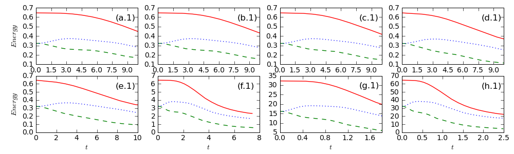
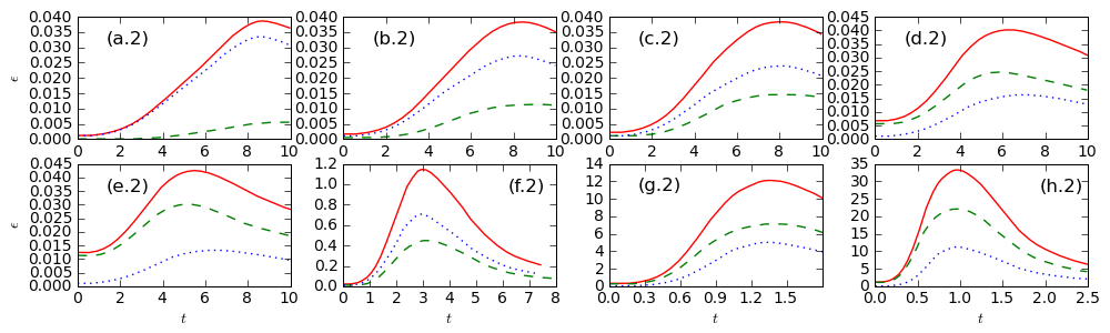
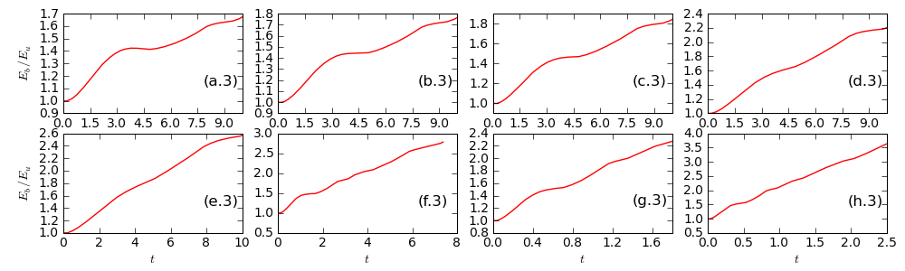
Figure 6: Plots versus time $t$ (given as a product of the number of iterations and the time step $\delta t$) of energies (a.1)-(h.1); total energy $E$ (red full line), kinetic-energy $E_{u}$ (green dashed line), and magnetic-energy $E_{b}$ (blue dotted line), of energy-dissipation rates (a.2)-(h.2); mean energy dissipation rate $\epsilon$ (red, full line), kinetic-energy dissipation $\epsilon_{u}$ (green dashed line), and magnetic-energy dissipation rate $\epsilon_{b}$ (blue dotted line), and of the ratio $E_{b}/E_{u}$ (a.3)-(h.3), generically, for decaying simulations (a) ${\rm Pr_{M}}=0.1$ (R1), (b) ${\rm Pr_{M}}=0.5$ (R2), (c) ${\rm Pr_{M}}=1.0$ (R3), (d) ${\rm Pr_{M}}=5.0$ (R4), (e) ${\rm Pr_{M}}=10.0$ (R5), (f) ${\rm Pr_{M}}=1.0$ (R3B), (g) ${\rm Pr_{M}}=5.0$ (R4B), and (h) ${\rm Pr_{M}}=10.0$ (R5B).

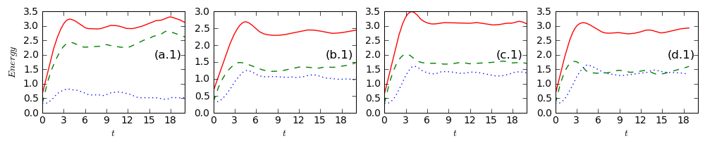
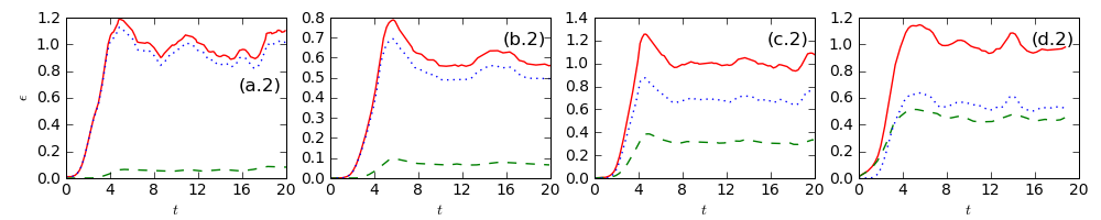
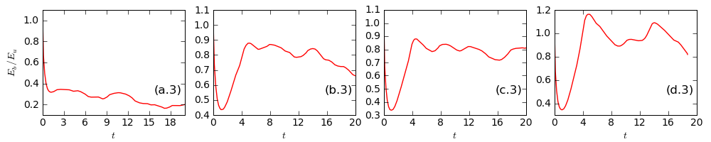
Figure 7: Plots versus time $t$ (given as a product of the number of iterations and the time step $\delta t$) of energies (a.1)-(d.1); total energy $E$ (red full line), kinetic-energy $E_{u}$ (green dashed line), and magnetic-energy $E_{b}$ (blue dotted line), of energy-dissipation rates (a.2)-(d.2); mean energy dissipation rate $\epsilon$ (red, full line), kinetic-energy dissipation rate $\epsilon_{u}$ (green dashed line), and magnetic-energy dissipation rate $\epsilon_{b}$ (blue dotted line), and of the ratio $E_{b}/E_{u}$ (a.3)-(d.3), generically, for forced simulations (a) ${\rm Pr_{M}}=0.01$ (R1D), (b) ${\rm Pr_{M}}=0.1$ (R2D), (c) ${\rm Pr_{M}}=1.0$ (R3D), and (d) ${\rm Pr_{M}}=10$ (R4D).

3.2 Temporal evolution

We examine the time evolution of the energy, the energy-dissipation rates, and related quantities, first for decaying and then for statistically steady MHD turbulence.

Figure 6 shows how the total energy $E$ (red full line), the kinetic energy $E_{u}$ (green dashed line), and the magnetic energy $E_{b}$ (blue dotted line) evolve with time $t$ (given as a product of the number of iterations and the time step $\delta t$) for runs R1-R5 [Figs. 6(a.1)-6(e.1)] and runs R3B-R5B [Figs. 6(f.1)-6(h.1)] for decaying MHD turbulence. Figure 6 also shows similar plots for the mean energy dissipation rate $\epsilon$ (red full line), the mean kinetic-energy dissipation rate $\epsilon_{u}$ (green dashed line), and the mean magnetic-energy dissipation rate $\epsilon_{b}$ (blue dotted line) versus time $t$ for runs R1-R5 [Figs. 6(a.2)-6(e.2)] and runs R3B-R5B [Figs. 6(f.2)-6(h.2)]. In addition Fig. 6 depicts the time-evolution of the ratio $E_{b}/E_{u}$ for runs R1-R5 [Figs. 6(a.3)-6(e.3)] and runs R3B-R5B [Figs. 6(f.3)-6(h.3)]. We see from these figures that, for all the values of ${\rm Pr_{M}}$ we have used, the energies $E$ and $E_{u}$ decay gently with $t$ but $E_{b}$ rises initially such that the ratio $E_{b}/E_{u}$ rises, nearly monotonically, with $t$ over the times we have considered; this is an intriguing trend that does not seem to have been noticed earlier. The times over which we have carried out our DNS are comparable to the cascade-completion time $t_{c}$ that can be obtained from the peaks in the plots of $\epsilon$, $\epsilon_{u}$, and $\epsilon_{b}$ versus $t$ [Figs. 6(a.2)-6(h.2)]; by comparing these plots we see that, as we move from ${\rm Pr_{M}}=0.1$ to ${\rm Pr_{M}}=10$, with fixed $\eta$, we find that $(\epsilon_{u}-\epsilon_{b})$ and $(t_{b}-t_{u})$ grow from negative values to positive ones because $\epsilon_{u}$ increases with ${\rm Pr_{M}}$, where $t_{b}$ and $t_{u}$ are the positions of the cascade-completion maxima in $\epsilon_{b}$ and $\epsilon_{u}$, respectively. We do not pursue the time evolution of our system well beyond $t_{u}$ and $t_{b}$ because the integral scale begins to grow thereafter and, eventually, can become comparable to the linear size of the simulation domain [45].

Figures 7(a.1)-7(d.1), show how the total energy $E$ (red full line), the total kinetic energy $E_{u}$ (green dashed line), and the total magnetic energy $E_{b}$ (blue dotted line) evolve with time $t$ (given as a product of the number of iterations and the time step $\delta t$) for, respectively, runs R1D-R4D for forced and statistically steady MHD turbulence. Figures 7(a.2)-7(d.2), show similar plots for the mean energy dissipation rate $\epsilon$ (red full line), the mean kinetic-energy dissipation rate $\epsilon_{u}$ (green dashed line), and the mean magnetic-energy dissipation rate $\epsilon_{b}$ (blue dotted line) versus time $t$ for, respectively, runs R1D-R4D. And Figs. 7(a.3)-7(d.3), depict the time-evolution of the ratio $E_{b}/E_{u}$ for these runs. We see from these figures that a statistically steady state is established in which the energies $E$, $E_{u}$, and $E_{b}$, the dissipation rates $\epsilon$, $\epsilon_{u}$, and $\epsilon_{b}$, and the ratio $E_{b}/E_{u}$ fluctuate about their mean values (after initial transients have died out). The mean value of $E_{b}/E_{u}$ increases from about $0.2-0.3$ to $E_{b}/E_{u}\simeq 1$ as ${\rm Pr_{M}}$ increases from $0.01$ to $10$. Furthermore, the mean values of the dissipation rates $\epsilon_{u}$ and $\epsilon_{b}$ are such that $(\epsilon_{u}-\epsilon_{b})$ grows from a negative value $\simeq-1$ to a value close to zero as ${\rm Pr_{M}}$ increases from $0.01$ to $10$.

3.3 Spectra

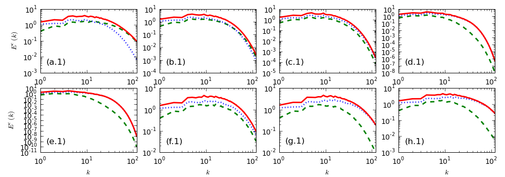
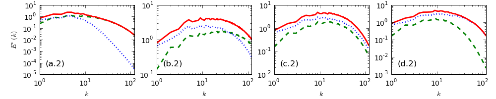
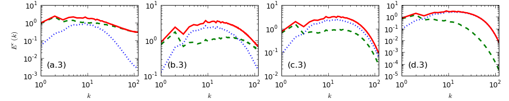
Figure 8: Log-log (base 10) plots of the compensated energy spectra $\epsilon^{-2/3}k^{5/3}E(k)$ (red full lines), $\epsilon_{-2/3}k^{5/3}E_{u}(k)$ (green dashed lines), and $\epsilon^{-2/3}k^{5/3}E_{b}(k)$ (blue dotted lines); on the vertical axes these are denoted generically as $E^{c}(k)$: (a.1) ${\rm Pr_{M}}=0.1$ (R1), (b.1) ${\rm Pr_{M}}=0.5$ (R2), (c.1) ${\rm Pr_{M}}=1.0$ (R3), (d.1) ${\rm Pr_{M}}=5.0$ (R4), (e.1) ${\rm Pr_{M}}=10.0$ (R5), (f.1) ${\rm Pr_{M}}=1.0$ (R3B), (g.1) ${\rm Pr_{M}}=5.0$ (R4B), (h.1) ${\rm Pr_{M}}=10.0$ (R5B), (a.2) ${\rm Pr_{M}}=0.01$ (R1C), (b.2) ${\rm Pr_{M}}=0.1$ (R2C), (c.2) ${\rm Pr_{M}}=1.0$ (R3C), and (d.2) ${\rm Pr_{M}}=10.0$ (R4C) for decaying MHD turbulence; and for statistically steady MHD turbulence (a.3) ${\rm Pr_{M}}=0.01$ (R1D), (b.3) ${\rm Pr_{M}}=0.1$ (R2D), (c.3) ${\rm Pr_{M}}=1.0$ (R3D), and (d.3) ${\rm Pr_{M}}=10.0$ (R4D).

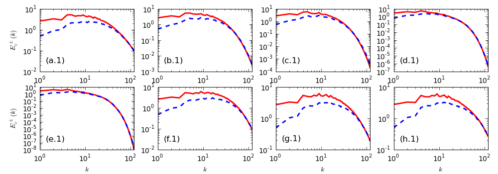
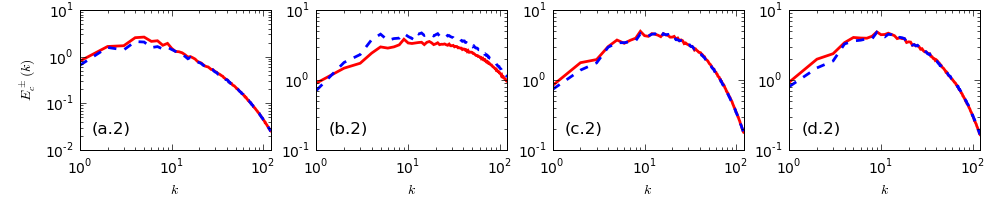
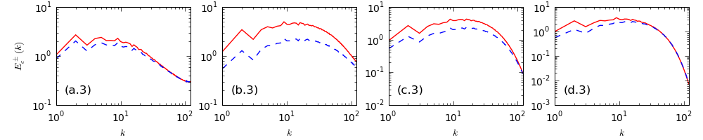
Figure 9: Log-log (base 10) plots of compensated energy spectra, $E_{c}^{\pm}(k)=k^{5/3}E^{\pm}(k)$, with $k$ the magnitude of the wave vector, for the Elsässer variables fields $z^{+}$ (red full line) and $z^{-}$ (blue dashed line): (a.1) ${\rm Pr_{M}}=0.1$ (R1), (b.1) ${\rm Pr_{M}}=0.5$ (R2), (c.1) ${\rm Pr_{M}}=1.0$ (R3), (d.1) ${\rm Pr_{M}}=5.0$ (R4), (e.1) ${\rm Pr_{M}}=10.0$ (R5), (f.1) ${\rm Pr_{M}}=1.0$ (R3B), (g.1) ${\rm Pr_{M}}=5.0$ (R4B), (h.1) ${\rm Pr_{M}}=10.0$ (R5B), (a.2) ${\rm Pr_{M}}=0.01$ (R1C), (b.2) ${\rm Pr_{M}}=0.1$ (R2C), (c.2) ${\rm Pr_{M}}=1.0$ (R3C), and (d.2) ${\rm Pr_{M}}=10.0$ (R4C) for decaying MHD turbulence; and for statistically steady MHD turbulence (a.3) ${\rm Pr_{M}}=0.01$ (R1D), (b.3) ${\rm Pr_{M}}=0.1$ (R2D), (c.3) ${\rm Pr_{M}}=1.0$ (R3D), and (d.3) ${\rm Pr_{M}}=10.0$ (R4D).

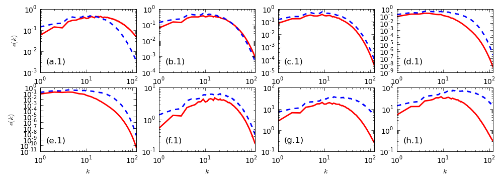
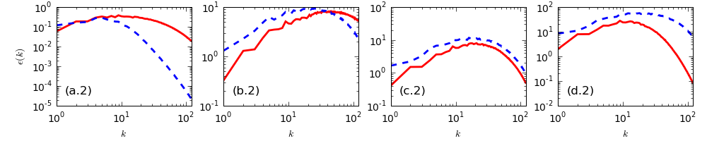
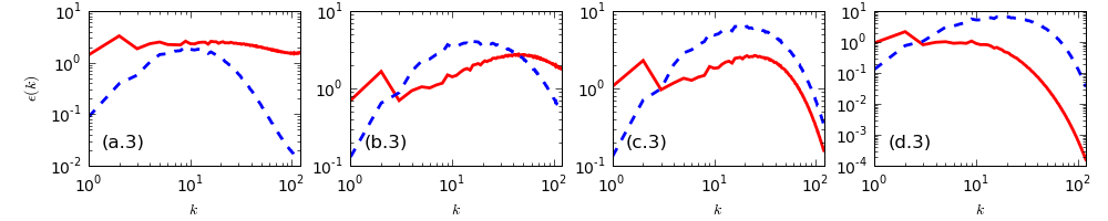
Figure 10: Log-log (base 10) plots of energy-dissipation spectra for the fluid (red full lines) and magnetic (blue dashed lines) fields, with $k$ the magnitude of the wave vector: (a.1) ${\rm Pr_{M}}=0.1$ (R1), (b.1) ${\rm Pr_{M}}=0.5$ (R2), (c.1) ${\rm Pr_{M}}=1.0$ (R3), (d.1) ${\rm Pr_{M}}=5.0$ (R4), (e.1) ${\rm Pr_{M}}=10.0$ (R5), (f.1) ${\rm Pr_{M}}=1.0$ (R3B), (g.1) ${\rm Pr_{M}}=5.0$ (R4B), (h.1) ${\rm Pr_{M}}=10.0$ (R5B), (a.2) ${\rm Pr_{M}}=0.01$ (R1C), (b.2) ${\rm Pr_{M}}=0.1$ (R2C), (c.2) ${\rm Pr_{M}}=1.0$ (R3C), and (d.2) ${\rm Pr_{M}}=10.0$ (R4C) for decaying MHD turbulence; and for statistically steady MHD turbulence (a.3) ${\rm Pr_{M}}=0.01$ (R1D), (b.3) ${\rm Pr_{M}}=0.1$ (R2D), (c.3) ${\rm Pr_{M}}=1.0$ (R3D), and (d.3) ${\rm Pr_{M}}=10.0$ (R4D).

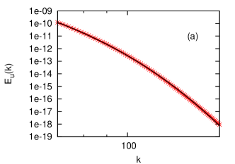
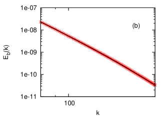
Figure 11: (a) The kinetic energy spectrum $E_{u}(k)$ (red asterisks) deep in the dissipation range for run R5; the black line indicates the fit $E_{u}(k)\sim k^{2.68}\exp(-0.235~{}k)$ for $5k^{u}_{d}<k<10k^{u}_{d}$, where $k^{u}_{d}=1/\eta_{d}^{u}$; (b) the magnetic energy spectrum $E_{b}(k)$ (red asterisks) deep in the dissipation range for run R1C; the black line indicates the fit $E_{b}(k)\sim k^{-5.24}\exp(-0.014~{}k)$ for $5k^{b}_{d}<k<10k^{b}_{d}$, where $k^{b}_{d}=1/\eta_{d}^{b}$.

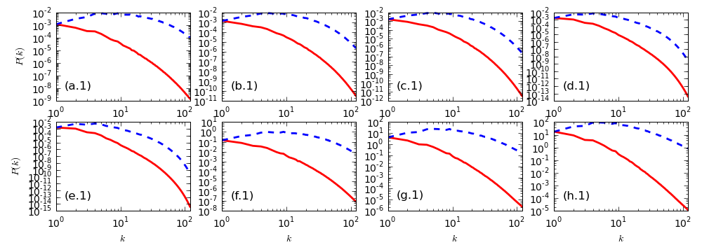
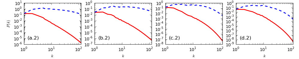
Figure 12: Log-log (base 10) plots of effective pressure spectra $P(k)$ (red full lines), with $k$ the magnitude of the wave vector, and the corresponding compensated spectra $P(k)k^{7/3}$ (blue, dashed lines): (a.1) ${\rm Pr_{M}}=0.1$ (R1), (b.1) ${\rm Pr_{M}}=0.5$ (R2), (c.1) ${\rm Pr_{M}}=1.0$ (R3), (d.1) ${\rm Pr_{M}}=5.0$ (R4), (e.1) ${\rm Pr_{M}}=10.0$ (R5), (f.1) ${\rm Pr_{M}}=1.0$ (R3B), (g.1) ${\rm Pr_{M}}=5.0$ (R4B), (h.1) ${\rm Pr_{M}}=10.0$ (R5B), for decaying MHD turbulence; and for statistically steady MHD turbulence (a.2) ${\rm Pr_{M}}=0.01$ (R1D), (b.2) ${\rm Pr_{M}}=0.1$ (R2D), (c.2) ${\rm Pr_{M}}=1.0$ (R3D), and (d.2) ${\rm Pr_{M}}=10.0$ (R4D).

We now discuss the behaviours of the energy, kinetic-energy, magnetic-energy, Elsässer variable, dissipation-rate, and effective-pressure spectra, first for decaying and then for statistically steady MHD turbulence. In the former case, spectra are obtained at the cascade-completion time $t_{c}$; in the latter, they are averaged over the statistically steady state that we obtain.

We present compensated spectra of the total energy $E_{c}(k)=\epsilon^{-2/3}k^{5/3}E(k)$ (red full line), the kinetic energy $E_{c}^{u}(k)=\epsilon^{-2/3}k^{5/3}E_{u}(k)$ (green dashed line), and the total magnetic energy $E_{c}^{b}(k)=\epsilon^{-2/3}k^{5/3}E_{b}(k)$ (blue dotted line) at $t_{c}$ for runs R1-R5 [Figs. 8(a.1)-8(e.1)], R3B-R5B [Figs. 8(f.1)-8(h.1)], and R1C-R4C [Figs. 8(a.2)-8(d.2)] for decaying MHD turbulence; and runs R1D-R4D [Figs. 8(a.3)-8(d.3)] show these for statistically steady MHD turbulence. From Figs. 8(a.1)-8(e.1) and Table 1 we see that $\eta_{d}^{u}$ increases as we increase $\nu$ to increase ${\rm Pr_{M}}$, because the initial energy is the same for runs R1-R5, so the dissipation tail in $E_{c}^{u}(k)$ is drawn in towards smaller and smaller values of $k$ as we move from ${\rm Pr_{M}}=0.1$ to ${\rm Pr_{M}}=10$; between ${\rm Pr_{M}}=0.5$ and ${\rm Pr_{M}}=1$ the tails of $E_{c}^{u}(k)$ and $E_{c}^{b}(k)$ and eventually $E_{c}^{b}(k)$ dominates and becomes indistinguishable from $E_{c}(k)$ on the scales of Figs. 8(d.1) and 8(e.1). A comparison of Figs. 8(f.1)-8(h.1) shows that, if we increase ${\rm Pr_{M}}$ from $1$ to $10$, we can keep both $k_{\rm max}\eta_{d}^{u}$ and $k_{\rm max}\eta_{d}^{b}$ close to $1$ so the dissipation ranges of these spectra span comparable ranges of $k$; however, as ${\rm Pr_{M}}$ increases, more and more of the energy is concentrated in the magnetic field. These trends are not affected (a) if we increase the number of collocation points, as can be seen from the compensated spectra in Figs. 8(a.2)-8(d.2) for runs R1C-R4C, which use $1024^{3}$ collocation points, or (b) if we study energy spectra for statistically steady MHD turbulence as can be seen from the compensated spectra in Figs. 8(a.3)-8(d.3) for runs R1D-R4D. Figures 8(c.1), 8(g.1), 8(c.2), and 8(c.3), for runs R3 (${\rm Re}_{\lambda}=121$), R3B (${\rm Re}_{\lambda}=210$), R3C (${\rm Re}_{\lambda}=172$), and R3D (${\rm Re}_{\lambda}=239$), respectively, all lie in one column and all have ${\rm Pr_{M}}=1$; so they provide a convenient way of comparing the ${\rm Re}_{\lambda}$ dependence of these spectra with a fixed value of ${\rm Pr_{M}}=1$. All the spectra in subfigures of Fig. 8 have been compensated by the $5/3$ power of $k$ and, to the extent that they show small, flat parts, their inertial-range, energy-spectra scalings are consistent with $k^{-5/3}$ behaviours; other powers, such as $-3/2$, can also give small, flat parts in compensated spectra. A detailed error analysis is required to decide which power is most consistent with our data; we defer such an error analysis to the Subsection 3.5 where we carry it out for structure functions.

Compensated spectra of the Elsässer variables, namely, $E^{+}_{c}(k)=\epsilon^{-2/3}k^{5/3}E^{+}(k)$ (red full lines) and $E^{-}_{c}(k)=\epsilon_{u}^{-2/3}k^{5/3}E^{-}(k)$ (blue dashed lines) are shown, at the cascade-completion time $t_{c}$, for the decaying-MHD-turbulence runs R1-R5 in Figs. 9(a.1)-9(e.1), R3B-R5B in Figs. 9(f.1)-9(h.1), and R1C-R4C in Figs. 9(a.2)-9(d.2); and Figs. 8(a.3)-9(d.3) show these spectra for statistically steady MHD turbulence in runs R1D-R4D, respectively. Note that the dissipation ranges of $E^{+}_{c}(k)$ and $E^{-}_{c}(k)$ overlap nearly on the scales of these figures. Differences between these are most pronounced at small $k$, where, typically, $E^{-}_{c}(k)$ lies below $E^{+}_{c}(k)$; these differences decrease with increasing ${\rm Pr_{M}}$, if we hold the initial energy fixed as in Figs. 9(a.1)-9(e.1) for runs R1-R5.

Next we come to the energy-dissipation (or enstrophy) spectra $\epsilon_{u}(k)=k^{2}E_{u}(k)$ (red full line) and $\epsilon_{b}(k)=k^{2}E_{b}(k)$ (blue dashed line) at $t_{c}$. These are shown, at the cascade-completion time $t_{c}$, for the decaying-MHD-turbulence runs R1-R5 in Figs. 10(a.1)-10(e.1), R3B-R5B in Figs. 10(f.1)-10(h.1), and R1C-R4C in Figs. 10(a.2)-10(d.2); and Figs. 10(a.3)-10(d.3) depict these spectra for statistically steady MHD-turbulence runs R1D-R4D. To the extent that most of these spectra show maxima at values of $k$ at the beginning of the dissipation range, most of our runs have well-resolved dissipation ranges; this also follows from the values of $k_{\rm max}\eta_{d}^{u}$ and $k_{\rm max}\eta_{d}^{b}$ in Table 1. Runs R1D and R2D have slightly under-resolved fluid-dissipation ranges with $k_{\rm max}\eta_{d}^{u}\simeq 0.32$ and $0.33$, respectively; and, for the former, a barely discernible, dissipation-range maximum in $\epsilon_{u}(k)$; however, as shown in our Navier-Stokes DNS in Subsection 3.1, reasonable results can be obtained for various statistical properties with $k_{\rm max}\eta_{d}^{u}\simeq 0.3$. The elucidation of the behaviours of dissipation-range spectra of course require large values of $k_{\rm max}\eta_{d}^{u}$ or $k_{\rm max}\eta_{d}^{b}$; in particular, runs R5 and R1C, with $k_{\rm max}\eta_{d}^{u}\simeq 13.3$ and $k_{\rm max}\eta_{d}^{b}\simeq 22.1$, respectively, are well suited for uncovering the functional forms of $E_{u}(k)$ and $E_{b}(k)$ in their dissipation ranges. In Figs. 11(a) and 11(b) we show, respectively, the kinetic- and magnetic-energy spectra $E_{u}(k)$ and $E_{b}(k)$ deep in their dissipation ranges for runs R5 and R1, respectively; our data for these spectra can be fit to the form $\sim k^{\alpha}\exp(-\beta k)$ for $k$ deep in the dissipation range and $\alpha$ and $\beta$ nonuniversal numbers that depend on the parameters of the simulation; similar results have been obtained for fluid turbulence [61, 64]. In particular, our data [Figs. 11(a) and 11(b)] for runs R5 and R1C are consistent with $E_{u}(k)\sim k^{2.68}\exp(-0.235~{}k)$, for $5k^{u}_{d}<k<10k^{u}_{d}$ with $k^{u}_{d}=1/\eta_{d}^{u}$, and $E_{b}(k)\sim k^{-5.24}\exp(-0.014~{}k)$, for $5k^{b}_{d}<k<10k^{b}_{d}$ with $k^{b}_{d}=1/\eta_{d}^{b}$, respectively.

We now turn to the spectra for the effective pressure $P(k)$ (red full lines) and their compensated versions $k^{7/3}P(k)$ (blue dashed lines) that are shown at $t_{c}$ for runs R1-R5 [Figs. 12(a.1)-12(e.1)] and R3B-R5B [Figs. 12(f.1)-12(h.1)] for decaying MHD turbulence; and for statistically steady MHD turbulence they are shown in Figs. 12(a.2)-12(d.2) for runs R1D-R4D. Pressure spectra have been studied for fluid turbulence as, e.g., in Refs. [46, 67]; to the best of our knowledge they have not been obtained for MHD turbulence. The compensated spectra here show that, for all our runs, the inertial-range behaviours of these effective-pressure spectra are consistent with the power law $k^{-7/3}$; this is consistent with the $k^{-5/3}$ behaviours of the energy spectra discussed above. Furthermore, as ${\rm Pr_{M}}$ increases from $0.1$ to $10$ in runs R1-R5, $P(k)$ falls more and more rapidly as can be seen from the vertical scales in Figs. 12(a.1)-12(e.1).

3.4 Probability distribution functions

We calculate several PDFs to characterise the statistical properties of decaying and statistically steady MHD turbulence. In the former case, PDFs are obtained at the cascade-completion time $t_{c}$; in the latter, they are averaged over the statistically steady state that we obtain. The PDFs we consider are of two types: the first type are PDFs of the cosines of angles between various vectors, such as ${\bf u}$ and ${\bm{\omega}}$; these help us to quantify the degrees of alignment between such vectors; the second type are PDFs of quantities such as $\epsilon_{u}$, $\epsilon_{b}$, and the eigenvalues of the rate-of-strain tensor.

In Fig. 13 we show plots of the PDFs of cosines of the angles between the vorticity ${\bm{\omega}}$ and the eigenvectors of the fluid rate-of-strain tensor $\mathbb{S}$, namely, $\hat{e}^{1}_{u}$ (red full line), $\hat{e}^{2}_{u}$ (green dashed lines), and $\hat{e}^{3}_{u}$ (blue dotted lines) for runs R1-R5 and R3B-R5B at the cascade-completion time $t_{c}$ for the case of decaying MHD turbulence. In Fig. 14 we show similar plots of the PDFs of cosines of the angles between the current density ${\bf j}$ and the eigenvectors of the fluid rate-of-strain tensor $\mathbb{S}$. The most important features of these figures are sharp peaks in the green dashed lines; these show that there is a marked tendency for the alignment or antialignment of ${\bm{\omega}}$ and $\hat{e}^{2}_{u}$, as in fluid turbulence, and of a similar tendency for the alignment or antialignment of ${\bf j}$ and $\hat{e}^{2}_{u}$; these features do not depend very sensitively on ${\rm Pr_{M}}$. Furthermore, the PDFs of cosines of the angles between ${\bm{\omega}}$ and $\hat{e}^{1}_{u}$ (blue dotted lines) and ${\bm{\omega}}$ and $\hat{e}^{3}_{u}$ (red full lines) show peaks near zero in Fig. 13; in contrast, analogous PDFs for the cosines of the angles between ${\bf j}$ and $\hat{e}^{1}_{u}$ (red full lines) and ${\bm{\omega}}$ and $\hat{e}^{3}_{u}$ (blue dotted lines) show nearly flat plateaux in the middle with very gentle maxima near $-0.5$ and $0.5$ [Fig. 14]. Runs R1C-R4C and R1D-R4D yield similar PDFs, for the cosines of these angles, so we do not give them here.

Plots of the PDFs of cosines of the angles between the velocity ${\bf u}$ and the eigenvectors of the fluid rate-of-strain tensor $\mathbb{S}$ are given Fig. 15; their analogues for ${\bf b}$ are given Fig. 16. Again, the most prominent features of these figures are sharp peaks in the green dashed lines; these show that there is a marked tendency for the alignment or antialignment of ${\bf u}$ and $\hat{e}^{2}_{u}$ and of a similar tendency for the alignment or antialignment of ${\bf j}$ and $\hat{e}^{2}_{u}$; these features do not depend very sensitively on ${\rm Pr_{M}}$. The PDFs of cosines of the angles between ${\bf u}$ and $\hat{e}^{1}_{u}$ (red full line) and ${\bf u}$ and $\hat{e}^{3}_{u}$ (blue dotted lines) show gentle, broad peaks that imply a weak preference for angles close to $45^{\circ}$ or $135^{\circ}$; these peaks are suppressed as we increase ${\rm Pr_{M}}$ [Figs. 15(a.1)-15(e.1) for runs R1-R5] with fixed initial energy, but they reappear if we compensate for the increase of ${\rm Pr_{M}}$ by increasing the initial energy [Figs. 15(f.1)-15(h.1)]. Similar, but sharper, peaks appear in the PDFs of cosines of the angles between ${\bf u}$ and $\hat{e}^{1}_{u}$ (red full lines) and ${\bf u}$ and $\hat{e}^{3}_{u}$ (blue dotted lines); these show a weak preference for angles close to $47^{\circ}$ or $133^{\circ}$ [Fig. 16]. Some simulations of compressible MHD turbulence have noted the presence of such peaks [35] for ${\rm Pr_{M}}=1$.

Only one of the eigenvalues $\Lambda_{1}^{b}$ of the tensile magnetic stress tensor $\mathbb{T}$ is non-zero; and the corresponding eigenvector ${\hat{e}}_{b}^{1}$ is identically aligned with ${\bf b}$. Thus PDFs of cosines of angles between ${\bf u}$, ${\bm{\omega}}$, ${\bf j}$, and ${\bf b}$ and the eigenvectors of $\mathbb{T}$ are simpler than their counterparts for $\mathbb{S}$ and are not presented here.

Figure 17 shows plots of PDFs of cosines of angles, denoted generically by $\theta$, between (a) ${\bf u}$ and ${\bf b}$, (b) ${\bf u}$ and ${\bm{\omega}}$, (c) ${\bf u}$ and ${\bf j}$, (d) ${\bm{\omega}}$ and ${\bf j}$, (e) ${\bf b}$ and ${\bm{\omega}}$, and (f) ${\bf b}$ and ${\bf j}$ for runs R1 (red lines), R2 (green lines), R3 (blue lines), R4 (black lines), and R5 (cyan lines). These figures show the following: (a) ${\bf u}$ and ${\bf b}$ are more aligned than antialigned [this is related to the small, positive, mean values of $H_{C}$ (see below) in our runs R1-R5]; (b) ${\bf u}$ and ${\bm{\omega}}$ and more antialigned than aligned, as noted for decaying fluid turbulence with slight helicity in Refs. [46, 68]; (c) ${\bf u}$ and ${\bf j}$ show approximately equal tendencies for alignment and antialignment; (d) ${\bm{\omega}}$ and ${\bf j}$ display a greater tendency for alignment than antialignment; (e) ${\bf b}$ and ${\bm{\omega}}$ have approximately equal tendencies for alignment and antialignment; and (f) ${\bf b}$ and ${\bf j}$ are more antialigned than aligned.

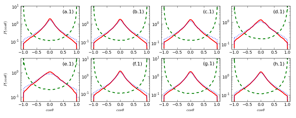
Figure 13: Semilog (base 10) plots of the PDFs of cosines of the angles, denoted generically by $\theta$, between the vorticity ${\bm{\omega}}$ and the eigenvectors of the fluid rate-of-strain tensor $\mathbb{S}$, namely, $\hat{e}^{1}_{u}$ (red full line),$\hat{e}^{2}_{u}$ (green dashed line), and $\hat{e}^{3}_{u}$ (blue dotted line): (a.1) ${\rm Pr_{M}}=0.1$ (R1), (b.1) ${\rm Pr_{M}}=0.5$ (R2), (c.1) ${\rm Pr_{M}}=1.0$ (R3), (d.1) ${\rm Pr_{M}}=5.0$ (R4), (e.1) ${\rm Pr_{M}}=10.0$ (R5), (f.1) ${\rm Pr_{M}}=1.0$ (R3B), (g.1) ${\rm Pr_{M}}=5.0$ (R4B), and (h.1) ${\rm Pr_{M}}=10.0$ (R5B) for decaying MHD turbulence.

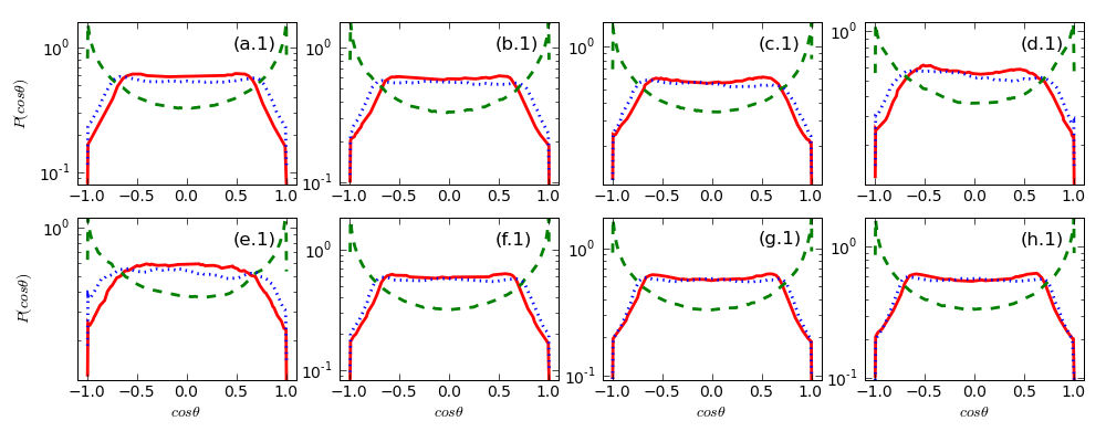
Figure 14: Semilog (base 10) plots of the PDFs cosines of angles, denoted generically by $\theta$, between the current density ${\bf j}$ and the eigenvectors of fluid rate-of-strain tensor $\mathbb{S}$, namely, $\hat{e}^{1}_{u}$ (red full line), $\hat{e}^{2}_{u}$ (green dashed line), and $\hat{e}^{3}_{u}$ (blue dotted line): (a.1) ${\rm Pr_{M}}=0.1$ (R1), (b.1) ${\rm Pr_{M}}=0.5$ (R2), (c.1) ${\rm Pr_{M}}=1.0$ (R3), (d.1) ${\rm Pr_{M}}=5.0$ (R4), (e.1) ${\rm Pr_{M}}=10.0$ (R5), (f.1) ${\rm Pr_{M}}=1.0$ (R3B), (g.1) ${\rm Pr_{M}}=5.0$ (R4B), and (h.1) ${\rm Pr_{M}}=10.0$ (R5B) for decaying MHD turbulence.

Figure 15: Semilog (base 10) plots of the PDFs of cosines of angles, denoted generically by $\theta$, between the velocity ${\bf u}$ and the eigenvectors of the fluid rate-of-strain tensor $\mathbb{S}$, namely, $\hat{e}^{1}_{u}$ (red full line), $\hat{e}^{2}_{u}$ (green dashed line), and $\hat{e}^{3}_{u}$ (blue dotted line): (a.1) ${\rm Pr_{M}}=0.1$ (R1), (b.1) ${\rm Pr_{M}}=0.5$ (R2), (c.1) ${\rm Pr_{M}}=1.0$ (R3), (d.1) ${\rm Pr_{M}}=5.0$ (R4), (e.1) ${\rm Pr_{M}}=10.0$ (R5), (f.1) ${\rm Pr_{M}}=1.0$ (R3B), (g.1) ${\rm Pr_{M}}=5.0$ (R4B), and (h.1) ${\rm Pr_{M}}=10.0$ (R5B) for decaying MHD turbulence.

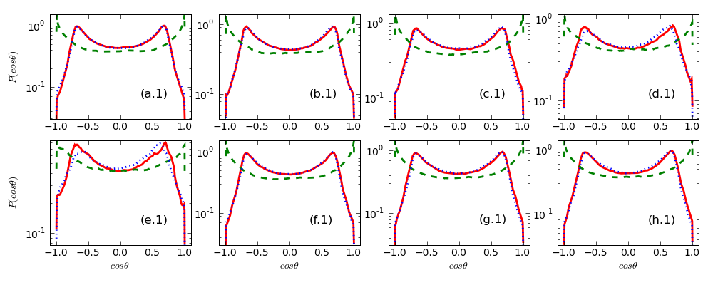
Figure 16: Semilog (base 10) plots of the PDFs of cosines of angles, denoted generically by $\theta$, between the magnetic field ${\bf b}$ and the eigenvectors of fluid rate-of-strain tensor $\mathbb{S}$, namely, $\hat{e}^{1}_{u}$ (red full line), $\hat{e}^{2}_{u}$ (green dashed line), and $\hat{e}^{3}_{u}$ (blue dotted line): (a.1) ${\rm Pr_{M}}=0.1$ (R1), (b.1) ${\rm Pr_{M}}=0.5$ (R2), (c.1) ${\rm Pr_{M}}=1.0$ (R3), (d.1) ${\rm Pr_{M}}=5.0$ (R4), (e.1) ${\rm Pr_{M}}=10.0$ (R5), (f.1) ${\rm Pr_{M}}=1.0$ (R3B), (g.1) ${\rm Pr_{M}}=5.0$ (R4B), and (h.1) ${\rm Pr_{M}}=10.0$ (R5B).

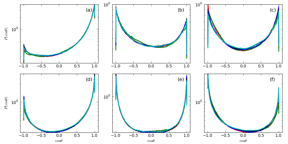
Figure 17: Semilog (base 10) plots of PDFs of cosines of angles, denoted generically by $\theta$, between (a) ${\bf u}$ and ${\bf b}$, (b) ${\bf u}$ and ${\bm{\omega}}$, (c) ${\bf u}$ and ${\bf j}$, (d) ${\bm{\omega}}$ and ${\bf j}$, (e) ${\bf b}$ and ${\bm{\omega}}$, and (f) ${\bf b}$ and ${\bf j}$ for runs R1 (red lines), R2 (green lines), R3 (blue lines), R4 (black lines), and R5 (cyan lines).

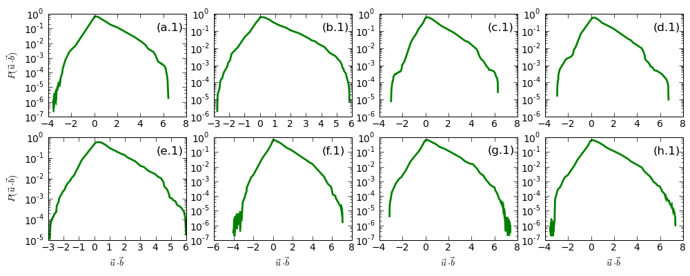
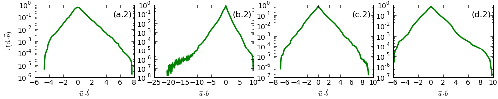
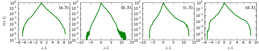
Figure 18: Semilog (base 10) plots of the PDFs of the cross helicity $H_{C}={\bf u}\cdot{\bf b}$ for (a.1) ${\rm Pr_{M}}=0.1$ (R1), (b.1) ${\rm Pr_{M}}=0.5$ (R2), (c.1) ${\rm Pr_{M}}=1.0$ (R3), (d.1) ${\rm Pr_{M}}=5.0$ (R4), (e.1) ${\rm Pr_{M}}=10.0$ (R5), (f.1) ${\rm Pr_{M}}=1.0$ (R3B), (g.1) ${\rm Pr_{M}}=5.0$ (R4B), (h.1) ${\rm Pr_{M}}=10.0$ (R5B), (a.2) ${\rm Pr_{M}}=0.01$ (R1C), (b.2) ${\rm Pr_{M}}=0.1$ (R2C), (c.2) ${\rm Pr_{M}}=1.0$ (R3C), and (d.2) ${\rm Pr_{M}}=10.0$ (R4C) for decaying MHD turbulence; and for statistically steady MHD turbulence (a.3) ${\rm Pr_{M}}=0.01$ (R1D), (b.3) ${\rm Pr_{M}}=0.1$ (R2D), (c.3) ${\rm Pr_{M}}=1.0$ (R3D), and (d.3) ${\rm Pr_{M}}=10.0$ (R4D); the arguments of the PDFs are scaled by their standard deviations $\sigma_{H_{C}}$.

Table 2: The mean $\mu_{H_{C}}$, standard deviation $\sigma_{H_{C}}$, skewness $\mu_{3,H_{C}}$, and kurtosis $\mu_{4,H_{C}}$ of the PDF of the cross helicity ${H_{C}}$ for our runs R1-R5 and R3B-R5B for decaying MHD turbulence at cascade completion; columns 6 and 7 give, respectively, the mean energy $E$ and ratio of the means of the cross helicity and the energy, i.e., $\mu_{H_{C}}/E$.

Run	$\mu_{H_{C}}$	$\sigma_{H_{C}}$	$\mu_{3,H_{C}}$	$\mu_{4,H_{C}}$	$E$	$\mu_{H_{C}}/E$
R1	0.118	0.173	1.103	4.901	0.461	0.256
R2	0.118	0.169	1.096	4.685	0.467	0.252
R3	0.120	0.170	1.096	4.679	0.490	0.245
R4	0.112	0.153	1.003	4.579	0.477	0.235
R5	0.105	0.141	0.934	4.324	0.460	0.228
R3B	1.217	1.804	1.100	4.912	4.909	0.248
R4B	5.915	8.766	1.097	4.917	24.50	0.241
R5B	11.50	17.05	1.102	5.000	48.32	0.238
R1C	0.014	0.113	0.615	5.748	0.358	0.041
R2C	-0.224	1.994	-0.698	8.441	5.440	-0.041
R3C	0.130	2.005	0.313	5.637	5.969	0.022
R4C	0.859	9.156	0.364	5.747	29.05	0.029
R1D	0.169	0.724	0.737	6.813	3.090	0.055
R2D	0.478	0.886	1.126	5.954	2.405	0.199
R3D	0.454	1.244	1.904	13.75	3.039	0.149
R4D	0.389	1.110	1.207	9.225	2.767	0.140

Probability distribution functions of the local cross helicity $H_{C}={\bf u}\cdot{\bf b}$ are shown via green full lines in Fig. 18. The arguments of these PDFs are scaled by their standard deviations, namely, $\sigma_{H_{C}}$; data for the PDFs are obtained at $t_{c}$ for runs R1-R5 in Figs. 18(a.1)-18(e.1), runs R3B-R5B in Figs. 18(f.1)-18(h.1), and runs R1C-R4C in Figs. 18(a.2)-18(d.2) for decaying MHD turbulence. For statistically steady MHD turbulence these PDFs are shown in Figs. 18(a.3)-18(d.3) for runs R1D-R4D. All these PDFs have peaks close to $H_{C}=0$; this reflects the tendency for ${\bf u}$ and ${\bf b}$ to be aligned or antialigned that we have discussed above. However, these PDFs are quite broad and distinctly non-Gaussian; this can be seen easily from the values of the mean $\mu_{H_{C}}$, standard deviation $\sigma_{H_{C}}$, skewness $\gamma_{3,H_{C}}$, and kurtosis $\gamma_{4,H_{C}}$ given in Table 2. Thus fluctuations of $H_{C}$ away from the mean are very significant. Table 2 also gives the value of the mean energy $E$ and the ratio $E/\mu_{H_{C}}$, which does not appear to be universal; for the runs R1-R5 and R3B-R5B it lies in the range $0.23$-$0.26$, for R1C-R2C in the range $-0.04$-$0.04$, and for R1D-R4D in the range $0.05$-$0.2$. For all our runs, with the exception of R2C, the mean $\mu_{H_{C}}$ and the skewness $\gamma_{3,H_{C}}$ are positive. Even if the PDF of $H_{C}$ had been a Gaussian, its mean value would have been within one standard deviation of 0; the actual PDF is much broader than a Gaussian. On symmetry grounds there is no reason for the system to display a nonzero value for $\mu_{H_{C}}$ unless there is some bias in the forcing or in the initial condition (the latter for the case of decaying turbulence). In any given run, if there is some residual $H_{C}$, it is reflected in a slight asymmetry in alignment (or antialignment) of ${\bf u}$ and ${\bf b}$, which we have studied above via the PDF of the cosine of the angle between ${\bf u}$ and ${\bf b}$. When we consider the ratio $\mu_{H_{C}}/E$ it seems to be substantial in some runs but, given the arguments above, we expect it to vanish in runs with a very large number of collocation points; indeed, it is very small in runs R1C-R4C.

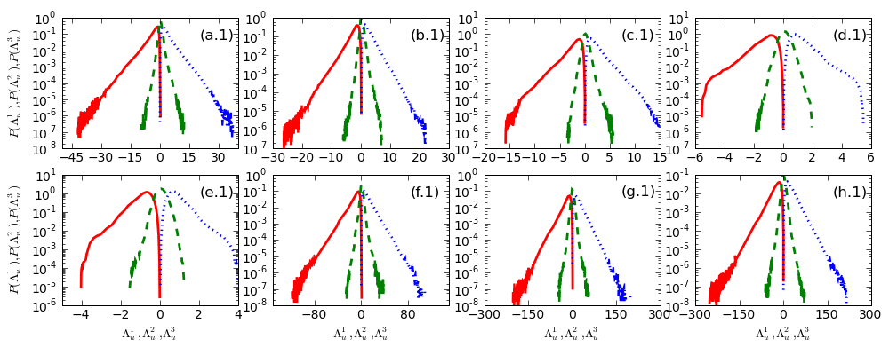
Figure 19: Semilog (base 10) plots of PDFs of the eigenvalues $\Lambda^{1}_{u}$ (blue dotted line), $\Lambda^{2}_{u}$ (green dashed line), and $\Lambda^{3}_{u}$ (red full line) of the rate-of-strain tensor $\mathbb{S}$ for (a.1) ${\rm Pr_{M}}=0.1$ (R1), (b.1) ${\rm Pr_{M}}=0.5$ (R2), (c.1) ${\rm Pr_{M}}=1.0$ (R3), (d.1) ${\rm Pr_{M}}=5.0$ (R4), (e.1) ${\rm Pr_{M}}=10.0$ (R5), (f.1) ${\rm Pr_{M}}=1.0$ (R3B), (g.1) ${\rm Pr_{M}}=5.0$ (R4B), and (h.1) ${\rm Pr_{M}}=10.0$ (R5B); the arguments of the PDFS are scaled by their standard deviations.

Consider now the PDFs of the eigenvalues $\Lambda^{1}_{u}$ (blue dotted line), $\Lambda^{2}_{u}$ (green dashed line), and $\Lambda^{3}_{u}$ (red full line) of the rate-of-strain tensor $\mathbb{S}$ shown in Figs. 19(a.1)-19(e.1) R1-R5 and Figs. 19(f.1)-19(h.1) for runs R3B-R5B. Recall that these eigenvalues provide measures of the local stretching and compression of the fluid; also we label the eigenvalues such that $\Lambda^{1}_{u}>\Lambda^{2}_{u}>\Lambda^{3}_{u}$. The incompressibility condition yields $\sum_{n=1}^{3}\Lambda^{n}_{u}=0$, whence it follows that $\Lambda^{1}_{u}>0$ and $\Lambda^{3}_{u}<0$; the intermediate eigenvalue $\Lambda^{2}_{u}$ can be either positive or negative. The illustrative plots in Figs. 19(a.1)-19(h.1) from our decaying-MHD-turbulence runs show that the PDFs of $\Lambda^{1}_{u}$ and $\Lambda^{3}_{u}$ have long tails on the right- and left-hand sides, respectively. These tails shrink as we increase ${\rm Pr_{M}}$ [Figs. 19(a.1)-19(e.1) for runs R1-R5, respectively], by increasing $\nu$ while holding the initial energy fixed; thus, there is a substantial decrease in regions of large strain. However, if we compensate for the increase in $\nu$ by increasing the energy in the initial condition such that $k_{\rm max}\eta_{d}^{u}$ and $k_{\rm max}\eta_{d}^{b}$ are both $\simeq 1$, we see that these tails stretch out, i.e., regions of large strain reappear.

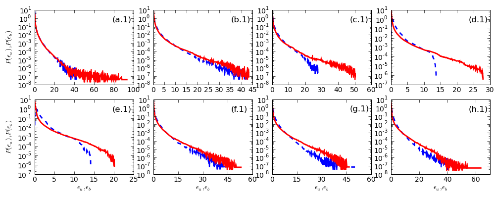
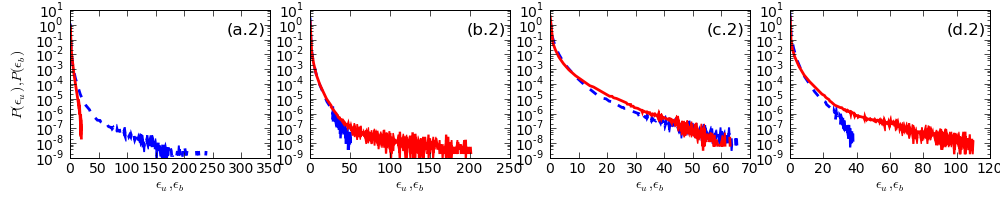
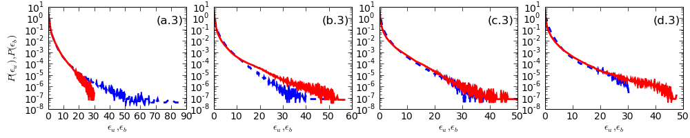
Figure 20: Semilog (base 10) plots of PDFs of the local kinetic-energy dissipation rate $\epsilon_{u}$ (blue dashed line) and the magnetic-energy dissipation rate $\epsilon_{b}$ (red full line), with the arguments scaled by their standard deviations, for: (a.1) ${\rm Pr_{M}}=0.1$ (R1), (b.1) ${\rm Pr_{M}}=0.5$ (R2), (c.1) ${\rm Pr_{M}}=1.0$ (R3), (d.1) ${\rm Pr_{M}}=5.0$ (R4), (e.1) ${\rm Pr_{M}}=10.0$ (R5), (f.1) ${\rm Pr_{M}}=1.0$ (R3B), (g.1) ${\rm Pr_{M}}=5.0$ (R4B), (h.1) ${\rm Pr_{M}}=10.0$ (R5B), (a.2) ${\rm Pr_{M}}=0.01$ (R1C), (b.2) ${\rm Pr_{M}}=0.1$ (R2C), (c.2) ${\rm Pr_{M}}=1.0$ (R3C), and (d.2) ${\rm Pr_{M}}=10.0$ (R4C) for decaying MHD turbulence; and for statistically steady MHD turbulence (a.3) ${\rm Pr_{M}}=0.01$ (R1D), (b.3) ${\rm Pr_{M}}=0.1$ (R2D), (c.3) ${\rm Pr_{M}}=1.0$ (R3D), and (d.3) ${\rm Pr_{M}}=10.0$ (R4D).

Table 3: The mean $\mu_{\epsilon_{u}}$, standard deviation $\sigma_{\epsilon_{u}}$, skewness $\gamma_{3,\epsilon_{u}}$, and kurtosis $\gamma_{4,\epsilon_{u}}$ of the PDFs of the local fluid energy dissipation $\epsilon_{u}$, and their analogues for $\epsilon_{b}$, for runs R1-R5, R3B-R5B, R1C-R4C, and R1D-R4D.

Run	$\mu_{\epsilon_{u}}$	$\sigma_{\epsilon_{u}}$	$\gamma_{3,\epsilon_{u}}$	$\gamma_{4,\epsilon_{u}}$	$\mu_{\epsilon_{b}}$	$\sigma_{\epsilon_{b}}$	$\gamma_{3,\epsilon_{b}}$	$\gamma_{4,\epsilon_{b}}$
R1	0.0048	0.0096	6.382	75.069	0.0302	0.0550	7.611	144.86
R2	0.0109	0.0187	6.053	70.566	0.0255	0.0527	8.182	121.47
R3	0.0141	0.0226	5.450	52.884	0.0233	0.0566	10.46	204.37
R4	0.0231	0.0284	4.042	28.306	0.0160	0.0397	7.955	97.662
R5	0.0273	0.0302	3.684	24.559	0.0130	0.0315	6.682	64.206
R3B	0.4165	0.7345	5.941	70.070	0.6440	1.5881	9.029	147.71
R4B	6.7843	10.898	5.343	55.676	4.4541	13.377	9.672	155.71
R5B	21.164	32.438	5.353	59.163	9.8332	31.177	9.621	151.64
R1C	0.0031	0.0076	18.45	1620.0	0.0566	0.0632	3.340	22.270
R2C	0.2354	0.5177	7.599	112.92	1.5655	3.5169	13.99	981.17
R3C	0.8349	1.6375	6.841	105.85	1.3186	3.5524	10.41	205.54
R4C	14.208	22.900	5.535	66.496	7.1624	24.974	13.33	406.21
R1D	0.0448	0.0630	5.799	89.678	0.8087	1.1004	4.587	40.328
R2D	0.0601	0.0933	5.180	51.311	0.4995	0.9808	8.488	142.97
R3D	0.2886	0.4233	5.230	55.366	0.6389	1.3120	6.755	80.154
R4D	0.4498	0.5536	5.055	58.832	0.5037	1.1391	8.077	129.65

We show PDFs of the kinetic-energy dissipation rate $\epsilon_{u}$ (blue dashed lines) and the magnetic-energy dissipation rate $\epsilon_{b}$ (red full lines) that are obtained at $t_{c}$ for runs R1-R5 in Figs. 20(a.1)-20(e.1), runs R3B-R5B in Figs. 20(f.1)-20(h.1), and runs R1C-R4C in Figs. 20(a.2)-20(d.2) for decaying MHD turbulence; and for statistically steady MHD turbulence they are shown in Figs. 20(a.3)-20(d.3) for runs R1D-R4D. All these PDFs have long tails; the tail of the PDF for $\epsilon_{b}$ extends further than the tail of that for $\epsilon_{u}$ for all except the smallest values of ${\rm Pr_{M}}$ [Figs. 20(a.1), 20(a.2), 20(a.3) for runs R1, R1C, and R1D, respectively]. This indicates that large values of $\epsilon_{b}$ are more likely to appear than large values of $\epsilon_{u}$ and, given the long tails of these PDFs, suggests that, except at the smallest values of ${\rm Pr_{M}}$ we have used, we might obtain more marked intermittency for the magnetic field than for the velocity field. Furthermore, as we expect, the tail of the PDF of $\epsilon_{u}$ is drawn in towards small values of $\epsilon_{u}$ as we increase ${\rm Pr_{M}}$ [Figs. 20(a.1)-20(e.1) for runs R1-R5, respectively] while holding $\eta$ and the initial energy fixed. However, if we compensate for the increase in $\nu$ by increasing the initial energy so that $k_{\rm max}\eta_{d}^{u}$ and $k_{\rm max}\eta_{d}^{b}$ are both $\simeq 1$, we see that the tails of the PDFs of $\epsilon_{b}$ and $\epsilon_{u}$ get elongated as we increase ${\rm Pr_{M}}$, e.g., in Figs. 20(f.1)-20(h.1) for runs R3B-R5B, respectively. The values of the mean $\mu_{\epsilon_{u}}$, standard deviation $\sigma_{\epsilon_{u}}$, skewness $\gamma_{3,\epsilon_{u}}$, and kurtosis $\gamma_{4,\epsilon_{u}}$ of the PDFs of the local fluid energy dissipation $\epsilon_{u}$ are given for all our runs and their counterparts for $\epsilon_{b}$ are given in Table 3. From these values we see that the right tails of these distributions fall much more slowly than the tail of a Gaussian distribution.

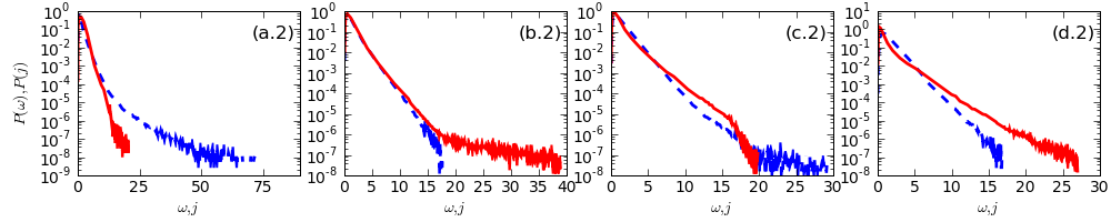
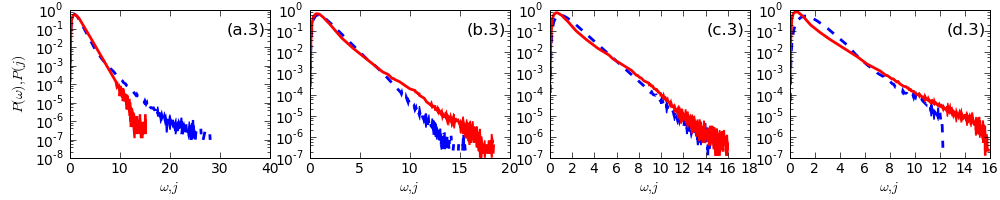
Figure 21: Semilog (base 10) plots of PDFs of the moduli of the local vorticity (blue dashed lines) and the current density (red full lines), $\omega$ and $j$, respectively, with the arguments of the PDFs scaled by their standard deviations, for (a.1) ${\rm Pr_{M}}=0.1$ (R1), (b.1) ${\rm Pr_{M}}=0.5$ (R2), (c.1) ${\rm Pr_{M}}=1.0$ (R3), (d.1) ${\rm Pr_{M}}=5.0$ (R4), (e.1) ${\rm Pr_{M}}=10.0$ (R5), (f.1) ${\rm Pr_{M}}=1.0$ (R3B), (g.1) ${\rm Pr_{M}}=5.0$ (R4B), (h.1) ${\rm Pr_{M}}=10.0$ (R5B), (a.2) ${\rm Pr_{M}}=0.01$ (R1C), (b.2) ${\rm Pr_{M}}=0.1$ (R2C), (c.2) ${\rm Pr_{M}}=1.0$ (R3C), and (d.2) ${\rm Pr_{M}}=10.0$ (R4C) for decaying MHD turbulence; and for statistically steady MHD turbulence (a.3) ${\rm Pr_{M}}=0.01$ (R1D), (b.3) ${\rm Pr_{M}}=0.1$ (R2D), (c.3) ${\rm Pr_{M}}=1.0$ (R3D), and (d.3) ${\rm Pr_{M}}=10.0$ (R4D).

Table 4: The mean $\mu_{\omega}$, standard deviation $\sigma_{\omega}$, skewness $\gamma_{3,\omega}$, and kurtosis $\gamma_{4,\omega}$ of the PDFs of the modulus of the local vorticity $\omega$, and their analogues for $j$, for runs R1-R5, R3B-R5B, R1C-R4C, and R1D-R4D.

Run	$\mu_{\omega}$	$\sigma_{\omega}$	$\gamma_{3,\omega}$	$\gamma_{4,\omega}$	$\mu_{j}$	$\sigma_{j}$	$\gamma_{3,j}$	$\gamma_{4,j}$
R1	3.817	3.138	2.174	10.25	3.109	2.340	2.206	11.42
R2	2.680	1.938	1.961	9.235	2.794	2.222	2.525	13.84
R3	2.189	1.512	1.871	8.598	2.606	2.215	2.873	17.16
R4	1.312	0.766	1.534	6.859	2.121	1.870	2.903	15.74
R5	1.022	0.567	1.363	6.098	1.906	1.695	2.789	13.95
R3B	11.50	8.706	1.949	8.908	13.27	12.06	2.791	15.61
R4B	21.30	14.98	1.828	8.246	32.58	34.11	3.243	19.05
R5B	26.93	18.23	1.770	8.049	47.08	51.90	3.360	19.79
R1C	25.31	23.10	2.265	11.17	21.00	18.47	2.456	14.56
R2C	15.70	13.07	2.062	9.831	18.35	17.95	2.899	17.01
R3C	21.68	15.49	1.746	7.910	38.85	45.50	3.563	23.00
R4C	2.945	2.661	3.027	26.37	1.446	0.861	1.451	6.816
R1D	12.14	8.700	2.297	14.16	5.336	3.456	1.702	7.683
R2D	14.26	9.802	1.745	7.821	12.58	9.544	2.336	12.64
R3D	10.07	6.544	1.644	7.463	13.88	11.24	2.320	11.36
R4D	4.119	2.349	1.388	6.526	11.92	10.47	2.429	12.46

Similar trends emerge if we examine the PDFs of the moduli of the vorticity and the current density, $\omega$ (blue dashed lines) and $j$ (red full lines), respectively: These are presented at $t_{c}$ for runs R1-R5 in Figs. 21(a.1)-21(e.1), runs R3B-R5B in Figs. 21(f.1)-21(h.1), and runs R1C-R4C in Figs. 21(a.2)-21(d.2) for decaying MHD turbulence; and for statistically steady MHD turbulence they are shown in Figs. 21(a.3)-21(d.3) for runs R1D-R4D. The tail of the PDF for $j$ extends further than the tail of that for $\epsilon_{u}$ for all except the smallest values of ${\rm Pr_{M}}$ [Figs. 21(a.1), 21(a.2), and 21(a.3) for runs R1, R1C, and R1D, respectively], so large values of $j$ are more likely than large values of $\omega$. Thus, given that these PDFs have long tails, it is reasonable to expect that, except at the smallest values of ${\rm Pr_{M}}$ we have used, intermittency for the magnetic field might be larger than that for the velocity field. Moreover, the tail of the PDF of $\omega$ is drawn in towards small values of $\omega$ as we increase ${\rm Pr_{M}}$ [Figs. 21(a.1)-21(e.1) for runs R1-R5, respectively] while holding $\eta$ and the initial energy fixed; but if, while increasing $\nu$, we also increase the initial energy so that $k_{\rm max}\eta_{d}^{u}$ and $k_{\rm max}\eta_{d}^{b}$ are $\simeq 1$, we see that the tails of the PDFs of $j$ and $\omega$ get stretched out as we increase ${\rm Pr_{M}}$, e.g., in Figs. 21(f.1)-21(h.1) for runs R3B-R5B, respectively. The values of the mean $\mu_{\omega}$, standard deviation $\sigma_{\omega}$, skewness $\gamma_{3,\omega}$, and kurtosis $\gamma_{4,\omega}$ of the PDFs of the modulus of the local vorticity $\omega$ for all our runs and their counterparts for $j$ are given in Table 4. From these values we see that the right tails of these distributions fall much more slowly than the tail of a Gaussian distribution.

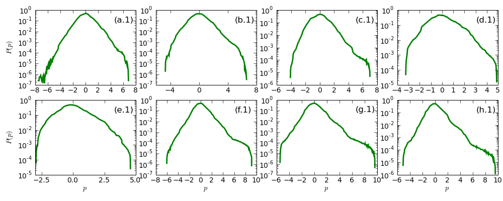
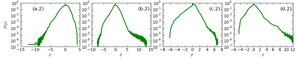
Figure 22: Semilog (base 10) plots of PDFs of local effective pressure fluctuations (green full lines), with the arguments of the PDFs scaled by their standard deviations, for (a.1) ${\rm Pr_{M}}=0.1$ (R1), (b.1) ${\rm Pr_{M}}=0.5$ (R2), (c.1) ${\rm Pr_{M}}=1.0$ (R3), (d.1) ${\rm Pr_{M}}=5.0$ (R4), (e.1) ${\rm Pr_{M}}=10.0$ (R5), (f.1) ${\rm Pr_{M}}=1.0$ (R3B), (g.1) ${\rm Pr_{M}}=5.0$ (R4B), (h.1) ${\rm Pr_{M}}=10.0$ (R5B), for decaying MHD turbulence; and for statistically steady MHD turbulence (a.2) ${\rm Pr_{M}}=0.01$ (R1D), (b.2) ${\rm Pr_{M}}=0.1$ (R2D), (c.2) ${\rm Pr_{M}}=1.0$ (R3D), and (d.2) ${\rm Pr_{M}}=10.0$ (R4D).

Table 5: The mean $\mu_{p}$, standard deviation $\sigma_{p}$, skewness $\gamma_{3,p}$, and kurtosis $\gamma_{4,p}$ of the PDFs of the local effective pressure $\bar{p}$ for runs R1-R5, R3B-R5B, and R1D-R4D.

Run	$\mu_{p}$	$\sigma_{p}$	$\gamma_{3,p}$	$\gamma_{4,p}$
R1	-3.283E-16	0.055	0.224	4.152
R2	-2.183E-16	0.057	0.256	4.052
R3	6.606E-16	0.061	0.315	3.722
R4	-2.787E-16	0.060	0.397	3.493
R5	-6.596E-16	0.059	0.433	3.527
R3B	2.975E-15	0.609	0.526	5.283
R4B	1.323E-14	3.184	0.660	5.645
R5B	-3.475E-14	6.397	0.719	5.776
R1D	9.014E-15	0.738	-0.533	3.882
R2D	1.136E-15	0.313	-0.153	4.697
R3D	1.244E-14	0.589	-1.066	5.338
R4D	9.983E-16	0.363	0.221	5.560

We move now to PDFs of the local effective pressure (green full lines), which are shown at $t_{c}$ for runs R1-R5 in Figs. 22(a.1)-22(e.1) and runs R3B-R5B in Figs. 22(f.1)-22(h.1) for decaying MHD turbulence; for statistically steady MHD turbulence they are shown in Figs. 22 a.2-d.2 for runs R1D-R4D. The values of the mean $\mu_{p}$, standard deviation $\sigma_{p}$, skewness $\gamma_{3,p}$, and kurtosis $\gamma_{4,p}$ of the PDFs of the local effective pressure $p$ are given for these runs in Table 5. These have mean $\mu_{p}=0$ but are distinctly non-Gaussian as can be seen from the values of $\gamma_{3,p}$ and $\gamma_{4,p}$. Pressure PDFs are negatively skewed in pure fluid turbulence as we have mentioned above; however, for MHD turbulence we find that the PDFs of the effective pressure $\bar{p}$ can be positively skewed, as in runs R1-R5, R3B-R5B, and run R4D, or negatively skewed, as in runs R1D-R3D; negative skewness seems to arise at low values of ${\rm Pr_{M}}$.

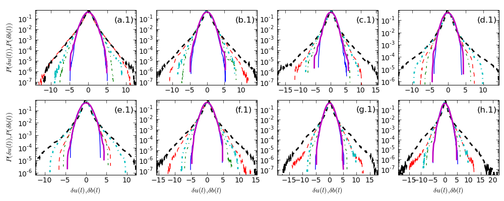
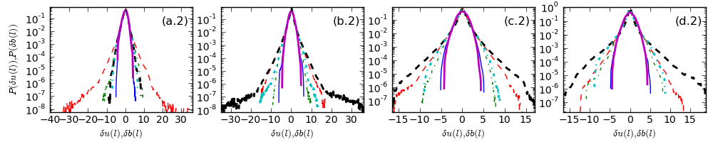
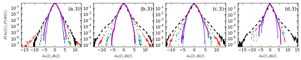
Figure 23: Semilog (base 10) plots of PDFs of velocity increments $\delta u(l)$, for separations $l=2\delta x$ (red dashed thin line), $10\delta x$ (green dot-dashed thin line), and $100\delta x$ (blue, full thin line), and of magnetic-field increments $\delta b(l)$, for separations $l=2\delta x$ (black dashed line), $10\delta x$ (cyan dot-dashed line), and $100\delta x$ (magenta full line), with the arguments of the PDFs scaled by their standard deviations, for (a.1) ${\rm Pr_{M}}=0.1$ (R1), (b.1) ${\rm Pr_{M}}=0.5$ (R2), (c.1) ${\rm Pr_{M}}=1.0$ (R3), (d.1) ${\rm Pr_{M}}=5.0$ (R4), (e.1) ${\rm Pr_{M}}=10.0$ (R5), (f.1) ${\rm Pr_{M}}=1.0$ (R3B), (g.1) ${\rm Pr_{M}}=5.0$ (R4B), (h.1) ${\rm Pr_{M}}=10.0$ (R5B), (a.2) ${\rm Pr_{M}}=0.01$ (R1C), (b.2) ${\rm Pr_{M}}=0.1$ (R2C), (c.2) ${\rm Pr_{M}}=1.0$ (R3C), and (d.2) ${\rm Pr_{M}}=10.0$ (R4C) for decaying MHD turbulence; and for statistically steady MHD turbulence (a.3) ${\rm Pr_{M}}=0.01$ (R1D), (b.3) ${\rm Pr_{M}}=0.1$ (R2D), (c.3) ${\rm Pr_{M}}=1.0$ (R3D), and (d.3) ${\rm Pr_{M}}=10.0$ (R4D).

The scale dependence of PDFs of velocity increments provides important clues about the nature of intermittency in fluid turbulence. To explore similar intermittency in MHD turbulence [72], we present data for the scale dependence of PDFs velocity and magnetic-field increments. As mentioned above, these increments are of the form $\delta a_{\parallel}({\bf x},l)\equiv{\bf a}({\bf x}+{\bf l},t)-{\bf a}({\bf x},t)]\cdot\frac{{\bf l}}{l}$, with ${\bf a}$ either ${\bf u}$ or ${\bf b}$, $l=|{\bf l}|$ the length scale, and ${\bf x}$ an origin over which we can average to determine the dependence of the PDFs of $\delta a_{\parallel}$ on the scale $l$; for notational convenience, such velocity and magnetic-field increments are denoted by $\delta u(l)$ and $\delta b(l)$ in our plots. These PDFs are obtained at $t_{c}$ for runs R1-R5 in Figs. 23(a.1)-23(e.1), runs R3B-R5B in Figs. 23(f.1)-23(h.1), and runs R1C-R4C in Figs. 23(a.2)-23(d.2) for decaying MHD turbulence; and for statistically steady MHD turbulence they are shown in Figs. 23(a.3)-23(d.3) for runs R1D-R4D. The PDFs of velocity increments are shown for separations $l=2\delta x$ (red dashed thin line), $l=10\delta x$ (green dot-dashed thin line), and $l=100\delta x$ (blue full thin line), where $\delta x$ is our real-space lattice spacing; for PDFs of magnetic-field increments we also use the separations $l=2\delta x$ (black dashed line), $l=10\delta x$ (cyan dot-dashed line), and $l=100\delta x$ (magenta full line); the arguments of these PDFs are scaled by their standard deviations. As in fluid turbulence, we see that these PDFs are nearly Gaussian if the length scale $l$ is large. As $l$ decreases, the PDFs develop, long, non-Gaussian tails, a clear signature of intermittency. Furthermore, a comparison of the red and black dashed lines in these plots indicates that the PDFs of the magnetic-field increments are broader than their velocity counterparts in most of our runs; this suggests, as we had surmised from the PDFs of energy-dissipation rates given above, that the magnetic field displays stronger intermittency than the velocity field at all but the smallest values of ${\rm Pr_{M}}$ [Figs. 23(a.1), 23(a.2), and 23(a.3) for runs R1, R1C, and R1D]; the general trend that we notice from these figures is that the magnetic-field intermittency is stronger than that of the velocity field at large magnetic Prandtl numbers but the difference between these intermittencies decreases as ${\rm Pr_{M}}$ is lowered. We will try to quantify this when we present structure functions in Subsection 3.5.

3.5 Structure functions

We continue our elucidation of intermittency in MHD turbulence by studying the scale dependence of order-$p$ equal-time, velocity and magnetic-field longitudinal structure functions $S_{p}^{u}(l)\equiv\langle|\delta u_{\parallel}({\bf x},l)|^{p}\rangle$ and magnetic-field longitudinal structure functions $S_{p}^{b}(l)\equiv\langle|\delta b_{\parallel}({\bf x},l)|^{p}\rangle$, respectively, where $\delta u_{\parallel}({\bf x},l)\equiv[{\bf u}({\bf x}+{\bf l},t)-{\bf u}({\bf x},t)]\cdot\frac{{\bf l}}{l}$ and $\delta b_{\parallel}({\bf x},l)\equiv[{\bf b}({\bf x}+{\bf l},t)-{\bf b}({\bf x},t)]\cdot\frac{{\bf l}}{l}$. From these structure functions we also obtain the hyperflatnesses $F_{6}^{u}(r)=S_{6}^{u}(r)/[S_{2}^{u}(r)]^{3}$ and $F_{6}^{b}(r)=S_{6}^{b}(r)/[S_{2}^{b}(r)]^{3}$. For the inertial range $\eta_{d}^{u},\eta_{d}^{b}\ll l\ll L$, we expect $S_{p}^{u}(l)\sim l^{\zeta_{p}^{u}}$ and $S_{p}^{b}(l)\sim l^{\zeta_{p}^{b}}$, where $\zeta_{p}^{u}$ and $\zeta_{p}^{b}$ are inertial-range multiscaling exponents for velocity and magnetic fields, respectively; if these fields show multiscaling, we expect significant deviations from the K41 result $\zeta_{p}^{uK41}=\zeta_{p}^{bK41}=p/3$. [Note that we do not expect any Iroshnikov-Kraichnan [73] scaling because we have no mean magnetic field in our simulations.] Given large inertial ranges, the multiscaling exponents can be extracted from slopes of log-log plots of structure functions versus $l$. However, in practical calculations inertial ranges are limited, so we use the extended-self-similarity (ESS) procedure [39, 40] in which we determine the multiscaling exponent ratios $\zeta_{p}^{u}/\zeta_{3}^{u}$ and $\zeta_{p}^{b}/\zeta_{3}^{b}$, respectively, from slopes of log-log plots of (a) $S_{p}^{u}$ versus $S_{3}^{u}$ and (b) $S_{p}^{b}$ versus $S_{3}^{b}$; we refer to these as ESS plots. Our data for structure functions are averaged over $51$ and $400$ origins, respectively, for simulations with $512^{3}$ and $1024^{3}$ collocation points.

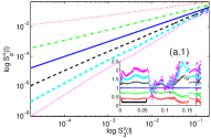
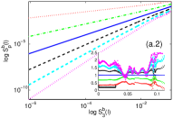
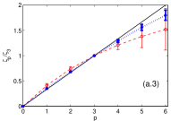
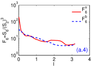
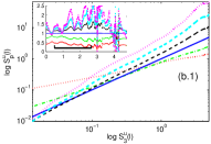
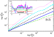
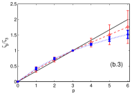
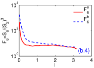
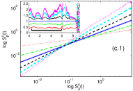
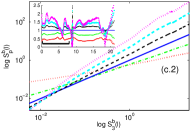
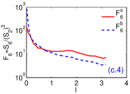
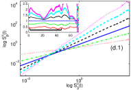
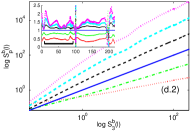
Figure 24: Log–log (base 10) ESS plots of order-$p$ structure functions of the velocity $S^{u}_{p}(l)$ [(a.1)-(d.1)] and magnetic-field $S^{b}_{p}(l)$ [(a.2)-(d.2)] versus $S^{u}_{3}(l)$ and $S^{b}_{3}(l)$, respectively; plots of the local slopes of these curves are shown in the inset. The black horizontal lines, with vertical ticks at their ends, show the inertial range over which we have averaged the exponent ratios $\zeta^{u}_{p}/\zeta_{p}^{u}$ and $\zeta^{u}_{p}/\zeta_{p}^{u}$; plots are shown for $p=1$ (red small-dotted line), $p=2$ (green dot-dashed line), $p=3$ (blue line), $p=4$ (black thin-dashed line), $p=5$ (cyan thick-dashed line), and $p=6$ (magenta large-dotted line). Subplots (a.3)-(d.3) show the exponent ratios $\zeta_{p}/\zeta_{3}$ versus $p$ for the velocity (red dashed line with thin errorbars) and magnetic fields (blue dotted line with thick errorbars); the black solid line shows the K41 result $\zeta_{p}^{K41}=p/3$. The semilog (base 10) plots (a.4)-(d.4) show the hyperflatnesses $F^{u}_{6}(l)$ (red line) and $F^{b}_{6}(l)$ (blue dashed line) versus $l$. Subplots in panels (a), (b), (c), and (d) are from our decaying-turbulence runs R1C, R2C, R3C, and R4C, respectively, with ${\rm Pr_{M}}=0.01,\,0.1,\,1$, and $10$.

Table 6: Multiscaling exponent ratios $\zeta_{p}^{u}/\zeta_{3}^{u}$ and $\zeta_{p}^{b}/\zeta_{3}^{b}$ from our decaying-MHD-turbulence runs R1C-R4C.

$p$	$\zeta_{p}^{u}/\zeta_{3}^{u}$; $\zeta_{p}^{b}/\zeta_{3}^{b}({\rm Pr_{M}}=0.01)$	$\zeta_{p}^{u}/\zeta_{3}^{u}$; $\zeta_{p}^{b}/\zeta_{3}^{b}({\rm Pr_{M}}=0.1)$
1	0.41 $\pm$ 0.04; 0.35 $\pm$ 0.01	0.39 $\pm$ 0.09; 0.42 $\pm$ 0.04
2	0.74 $\pm$ 0.04; 0.68 $\pm$ 0.01	0.71 $\pm$ 0.08; 0.74 $\pm$ 0.03
3	1.00 $\pm$ 0.00; 1.00 $\pm$ 0.00	1.00 $\pm$ 0.00; 1.00 $\pm$ 0.00
4	1.21 $\pm$ 0.09; 1.29 $\pm$ 0.03	1.26 $\pm$ 0.14; 1.20 $\pm$ 0.03
5	1.38 $\pm$ 0.22; 1.56 $\pm$ 0.06	1.51 $\pm$ 0.32; 1.37 $\pm$ 0.07
6	1.52 $\pm$ 0.41; 1.80 $\pm$ 0.10	1.76 $\pm$ 0.53; 1.52 $\pm$ 0.13
$p$	$\zeta_{p}^{u}/\zeta_{3}^{u}$; $\zeta_{p}^{b}/\zeta_{3}^{b}({\rm Pr_{M}}=1)$	$\zeta_{p}^{u}/\zeta_{3}^{u}$; $\zeta_{p}^{b}/\zeta_{3}^{b}({\rm Pr_{M}}=10)$
1	0.42 $\pm$ 0.03; 0.49 $\pm$ 0.04	0.40 $\pm$ 0.06; 0.50 $\pm$ 0.05
2	0.74 $\pm$ 0.03; 0.80 $\pm$ 0.04	0.72 $\pm$ 0.05; 0.81 $\pm$ 0.04
3	1.00 $\pm$ 0.00; 1.00 $\pm$ 0.00	1.00 $\pm$ 0.00; 1.00 $\pm$ 0.00
4	1.25 $\pm$ 0.06; 1.15 $\pm$ 0.07	1.27 $\pm$ 0.08; 1.15 $\pm$ 0.05
5	1.50 $\pm$ 0.16; 1.27 $\pm$ 0.18	1.55 $\pm$ 0.18; 1.29 $\pm$ 0.12
6	1.74 $\pm$ 0.30; 1.38 $\pm$ 0.32	1.83 $\pm$ 0.31; 1.45 $\pm$ 0.23

We begin with data from our decaying-MHD-turbulence runs R1C-R4C, which use $1024^{3}$ collocation points and span the ${\rm Pr_{M}}$ range $0.01-10$. Figures 24(a.1)-24(d.1) show ESS plots for $S^{u}_{p}(r)$ for runs R1C-R4C, respectively, for $p=1$ (red small-dotted line), $p=2$ (green dot-dashed line), $p=3$ (blue line), $p=4$ (black thin-dashed line), $p=5$ (cyan thick-dashed line), and $p=6$ (magenta large-dotted line); their analogues for $S^{b}_{p}(r)$ are given in Figs. 24(a.2)-24(d.2); the local slopes of these ESS curves are shown in the insets of these figures. Flat portions in these plots of local slopes help us to identify the inertial ranges. The regions that we have chosen for our fits are indicated by black horizontal lines with vertical ticks at their ends. In such a region, the mean value and the standard deviation of the local slope of the ESS plot for $S^{u}_{p}(r)$ (or $S^{b}_{p}(r)$) yield, respectively, our estimates for the exponent ratio $\zeta_{p}^{u}/\zeta_{3}^{u}$ (or $\zeta_{p}^{b}/\zeta_{3}^{b}$) and its errorbars. Figures 24(a.3)-24(d.3) show plots of these exponent ratios versus $p$ for the velocity field (blue dotted line with thick errorbars) and the magnetic field (red dashed line with thin error bars); the black solid line shows the K41 result for comparison. Though earlier studies [25, 38] have obtained such exponents from DNS studies, they have done so, to the best of our knowledge, only for ${\rm Pr_{M}}=1$; furthermore, they have not reported errorbars. Although our (conservative) errorbars are large, our plots of exponent ratios suggest the following: (a) deviations from the K41 result are significant, especially for $p>3$, as in fluid turbulence; (b) at large values of ${\rm Pr_{M}}$ the magnetic field is more intermittent than the velocity field, in so far as the deviations of $\zeta_{p}^{b}/\zeta_{3}^{b}$ from the K41 result $p/3$ are larger than those of $\zeta_{p}^{u}/\zeta_{3}^{u}$; (c) as we reduce ${\rm Pr_{M}}$ this difference in intermittency reduces until, at ${\rm Pr_{M}}=0.01$, the velocity field shows signs of becoming more intermittent than the magnetic field. This trend in intermittency is corroborated by plots versus $l$ of the the hyperflatnesses $F^{u}_{6}(l)=\frac{S^{u}_{6}(l)}{S^{u}_{2}(l)^{3}}$ (red line) and $F^{b}_{6}(l)=\frac{S^{b}_{6}(l)}{S^{b}_{2}(l)^{3}}$ (blue dashed line) in Figs. 24(a.4)-24(d.4) for runs R1C-R4C, respectively: As $l$ decreases, $F^{b}_{6}(l)$ rises more rapidly than $F^{u}_{6}(l)$ except at ${\rm Pr_{M}}=0.01$.

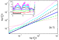
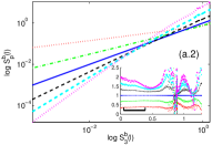
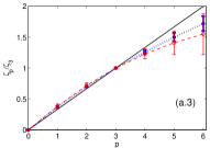
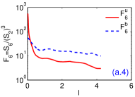
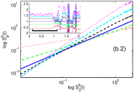
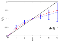
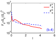
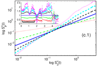
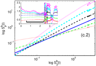
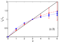
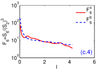
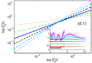
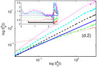
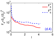
Figure 25: Log–log (base 10) ESS plots of order-$p$ structure functions of the velocity $S^{u}_{p}(l)$ [(a.1)-(d.1)] and magnetic-field $S^{b}_{p}(l)$ [(a.2)-(d.2)] versus $S^{u}_{3}(l)$ and $S^{b}_{3}(l)$, respectively; plots of the local slopes of these curves are shown in the inset. The black horizontal lines, with vertical ticks at their ends, show the inertial range over which we have averaged the exponent ratios $\zeta^{u}_{p}/\zeta_{p}^{u}$ and $\zeta^{u}_{p}/\zeta_{p}^{u}$; plots are shown for $p=1$ (red small-dotted line), $p=2$ (green dot-dashed line), $p=3$ (blue line), $p=4$ (black thin-dashed line), $p=5$ (cyan thick-dashed line), and $p=6$ (magenta large-dotted line). Subplots (a.3)-(d.3) show the exponent ratios $\zeta_{p}/\zeta_{3}$ versus $p$ for the velocity (red dashed line with thin errorbars) and magnetic fields (blue dotted line with thick errorbars); the black solid line shows the K41 result $\zeta_{p}^{K41}=p/3$. The semilog (base 10) plots (a.4)-(d.4) show the hyperflatnesses $F^{u}_{6}(l)$ (red line) and $F^{b}_{6}(l)$ (blue dashed line) versus $l$. Subplots in panels (a), (b), (c), and (d), are from our statistically steady MHD-turbulence runs R1D, R2D, R3D, and R4D, respectively, with ${\rm Pr_{M}}=0.01,\,0.1,\,1$, and $10$.

Table 7: Multiscaling exponent ratios $\zeta_{p}^{u}/\zeta_{3}^{u}$ and $\zeta_{p}^{b}/\zeta_{3}^{b}$ from our statistically steady MHD-turbulence runs R1D-R4D.

$p$	$\zeta_{p}^{u}/\zeta_{3}^{u}$; $\zeta_{p}^{b}/\zeta_{3}^{b}({\rm Pr_{M}}=0.01)$	$\zeta_{p}^{u}/\zeta_{3}^{u}$; $\zeta_{p}^{b}/\zeta_{3}^{b}({\rm Pr_{M}}=0.1)$
1	0.38 $\pm$ 0.04; 0.37 $\pm$ 0.01	0.42 $\pm$ 0.03; 0.52 $\pm$ 0.11
2	0.72 $\pm$ 0.04; 0.70 $\pm$ 0.01	0.74 $\pm$ 0.02; 0.83 $\pm$ 0.09
3	1.00 $\pm$ 0.00; 1.00 $\pm$ 0.00	1.00 $\pm$ 0.00; 1.00 $\pm$ 0.00
4	1.23 $\pm$ 0.08; 1.26 $\pm$ 0.03	1.20 $\pm$ 0.04; 1.12 $\pm$ 0.12
5	1.41 $\pm$ 0.19; 1.50 $\pm$ 0.07	1.36 $\pm$ 0.11; 1.24 $\pm$ 0.28
6	1.55 $\pm$ 0.33; 1.72 $\pm$ 0.12	1.49 $\pm$ 0.20; 1.39 $\pm$ 0.54
$p$	$\zeta_{p}^{u}/\zeta_{3}^{u}$; $\zeta_{p}^{b}/\zeta_{3}^{b}({\rm Pr_{M}}=1)$	$\zeta_{p}^{u}/\zeta_{3}^{u}$; $\zeta_{p}^{b}/\zeta_{3}^{b}({\rm Pr_{M}}=10)$
1	0.39 $\pm$ 0.04; 0.47 $\pm$ 0.02	0.37 $\pm$ 0.02; 0.51 $\pm$ 0.06
2	0.73 $\pm$ 0.04; 0.79 $\pm$ 0.01	0.71 $\pm$ 0.02; 0.82 $\pm$ 0.06
3	1.00 $\pm$ 0.00; 1.00 $\pm$ 0.00	1.00 $\pm$ 0.00; 1.00 $\pm$ 0.00
4	1.20 $\pm$ 0.10; 1.13 $\pm$ 0.02	1.25 $\pm$ 0.05; 1.11 $\pm$ 0.08
5	1.36 $\pm$ 0.30; 1.24 $\pm$ 0.06	1.47 $\pm$ 0.13; 1.18 $\pm$ 0.16
6	1.46 $\pm$ 0.52; 1.33 $\pm$ 0.12	1.65 $\pm$ 0.26; 1.25 $\pm$ 0.24

Similar results follow from our studies of statistically steady MHD turbulence in runs R1D-R4D, which use $512^{3}$ collocation points and span the ${\rm Pr_{M}}$ range $0.01-10$. Figures 25(a.1)-25(d.1) show ESS plots for $S^{u}_{p}(r)$ for runs R1D-R4D, respectively, for $p=1$ (red small-dotted line), $p=2$ (green dot-dashed line), $p=3$ (blue line), $p=4$ (black thin-dashed line), $p=5$ (cyan thick-dashed line), and $p=6$ (magenta large-dotted line); their analogues for $S^{b}_{p}(r)$ are given in Figs. 25(a.2)-25(d.2); the local slopes of these ESS curves are shown in the insets of these figures. We obtain estimates for the exponent ratio $\zeta_{p}^{u}/\zeta_{3}^{u}$ and $\zeta_{p}^{b}/\zeta_{3}^{b}$ and their errorbars as in Fig. 24. Figures 25(a.3)-25(d.3) show plots of these exponent ratios versus $p$ for the velocity field (blue dotted line with thick errorbars) and the magnetic field (red dashed line with thin errorbars); the black solid line shows the K41 result for comparison. Plots versus $l$ of the hyperflatnesses $F^{u}_{6}(l)$ (red line) and $F^{b}_{6}(l)$ (blue dashed line) are given in Figs. 25(a.4)-25(d.4) for runs R1D-R4D, respectively. All the trends here as exactly as in the decaying-MHD-turbulence plots in Fig. 24.

Tables 6 and 7 summarise, respectively, our results for multiscaling exponent ratios for our decaying-MHD-turbulence runs R1C-R4C and our statistically steady MHD-turbulence runs R1D-R4D. The trends of these ratios with ${\rm Pr_{M}}$ have been discussed above. By comparing corresponding entries in the columns and rows of these tables, we see that exponent ratios from decaying and statistically steady MHD turbulence agree, given our (conservative) error bars. Thus, at least at this level of resolution and accuracy, we have strong universality of these exponent ratios, for a given value of ${\rm Pr_{M}}$, in as much as the ratios from decaying-MHD turbulence agree with those from the statistically steady case. The dependence on ${\rm Pr_{M}}$ will be examined in Sec. 4.

Table 8: A comparison of multiscaling exponent ratios $\zeta_{p}^{u}/\zeta_{3}^{u}$ and $\zeta_{p}^{b}/\zeta_{3}^{b}$ from our statistically steady and decaying MHD simulations and from decaying MHD simulations by Mininni and Pouquet (Ref. [30]), for ${\rm Pr_{M}}=1$.

$p$	$\zeta^{u}_{p}$ Ref. [30]	$\zeta^{u}_{p}/\zeta^{u}_{3}$ Ref. [30]	$\zeta^{u}_{p}/\zeta^{u}_{3}$ (R3D)	$\zeta^{u}_{p}/\zeta^{u}_{3}$ (R3C)
1	0.30	0.40	0.39 $\pm$ 0.04	0.42 $\pm$ 0.03
2	0.55	0.74	0.73 $\pm$ 0.04	0.74 $\pm$ 0.03
3	0.74	1.00	1.00 $\pm$ 0.00	1.00 $\pm$ 0.00
4	0.91	1.22	1.20 $\pm$ 0.10	1.25 $\pm$ 0.06
5	1.04	1.39	1.36 $\pm$ 0.30	1.50 $\pm$ 0.16
6	1.17	1.56	1.46 $\pm$ 0.52	1.74 $\pm$ 0.30
$p$	$\zeta^{b}_{p}$ Ref. [30]	$\zeta^{b}_{p}/\zeta^{b}_{3}$ Ref. [30]	$\zeta^{b}_{p}/\zeta^{b}_{3}$ (R3D)	$\zeta^{b}_{p}/\zeta^{b}_{3}$ (R3C)
1	0.36	0.43	0.47 $\pm$ 0.02	0.49 $\pm$ 0.04
2	0.63	0.76	0.79 $\pm$ 0.01	0.80 $\pm$ 0.04
3	0.83	1.00	1.00 $\pm$ 0.00	1.00 $\pm$ 0.00
4	0.97	1.16	1.13 $\pm$ 0.02	1.15 $\pm$ 0.07
5	1.07	1.28	1.24 $\pm$ 0.06	1.27 $\pm$ 0.18
6	1.14	1.36	1.33 $\pm$ 0.12	1.38 $\pm$ 0.32

3.6 Isosurfaces

As we have mentioned in our discussion of fluid turbulence, isosurface plots of quantities such as $\omega$, the modulus of the vorticity, give us a visual appreciation of small-scale structures in a turbulent flow; in fluid turbulence, iso-$\omega$ surfaces are slender tubes if $\omega$ is chosen to be well above its mean value [65, 71]. For the case of MHD turbulence it is natural to consider isosurface plots [74] of $\omega$, the modulus $j$ of the current density, energy dissipation rates, and the effective pressure.

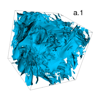
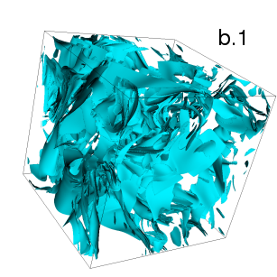
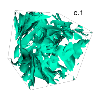
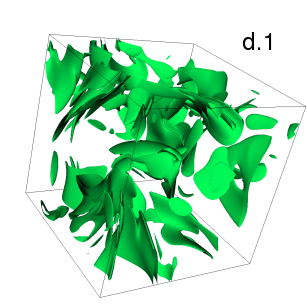
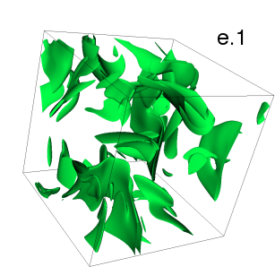
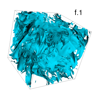
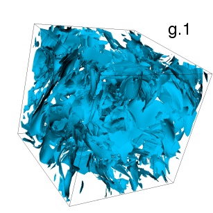
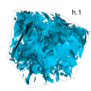
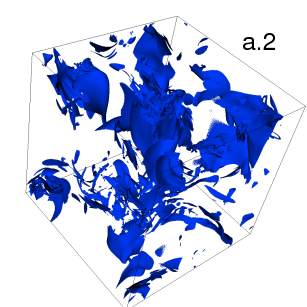
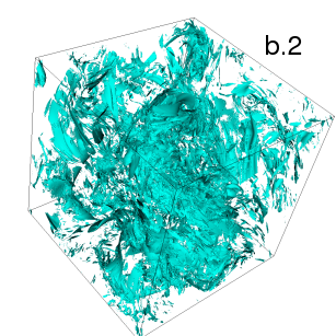
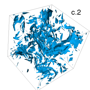
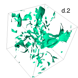
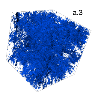
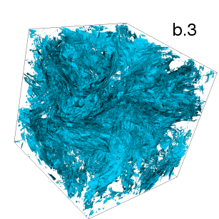
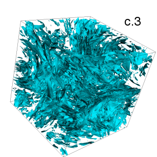
Figure 26: Isosurfaces of the modulus $\omega$ of the vorticity: (a.1) ${\rm Pr_{M}}=0.1$ (R1), (b.1) ${\rm Pr_{M}}=0.5$ (R2), (c.1) ${\rm Pr_{M}}=1.0$ (R3), (d.1) ${\rm Pr_{M}}=5.0$ (R4), (e.1) ${\rm Pr_{M}}=10.0$ (R5), (f.1) ${\rm Pr_{M}}=1.0$ (R3B), (g.1) ${\rm Pr_{M}}=5.0$ (R4B), (h.1) ${\rm Pr_{M}}=10.0$ (R5B), (a.2) ${\rm Pr_{M}}=0.01$ (R1C), (b.2) ${\rm Pr_{M}}=0.1$ (R2C), (c.2) ${\rm Pr_{M}}=1.0$ (R3C), and (d.2) ${\rm Pr_{M}}=10.0$ (R4C) for decaying MHD turbulence; and for statistically steady MHD turbulence (a.3) ${\rm Pr_{M}}=0.01$ (R1D), (b.3) ${\rm Pr_{M}}=0.1$ (R2D), (c.3) ${\rm Pr_{M}}=1.0$ (R3D), and (d.3) ${\rm Pr_{M}}=10.0$ (R4D); these isosurfaces go through points at which the value of $\omega$ is two standard deviations above its mean value (for any given plot).

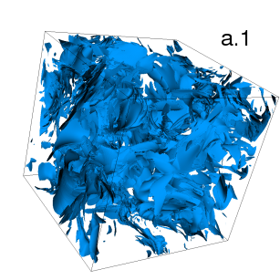
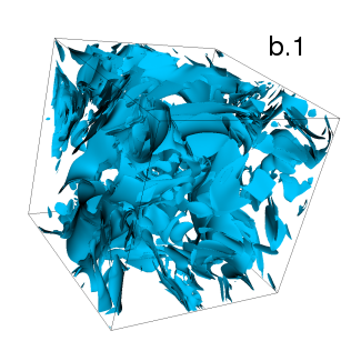
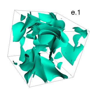
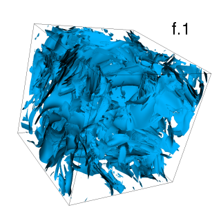
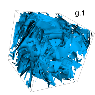
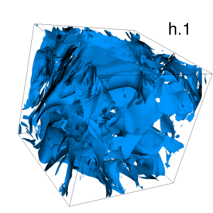
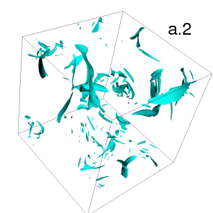
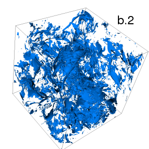
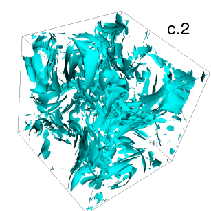
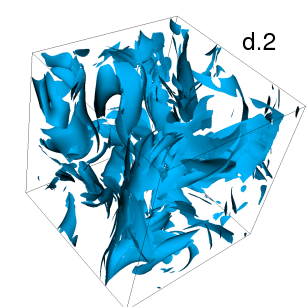
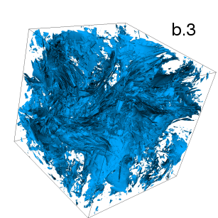
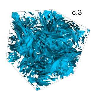
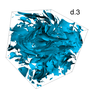
Figure 27: Isosurfaces of the modulus $j$ of the current density: (a.1) ${\rm Pr_{M}}=0.1$ (R1), (b.1) ${\rm Pr_{M}}=0.5$ (R2), (c.1) ${\rm Pr_{M}}=1.0$ (R3), (d.1) ${\rm Pr_{M}}=5.0$ (R4), (e.1) ${\rm Pr_{M}}=10.0$ (R5), (f.1) ${\rm Pr_{M}}=1.0$ (R3B), (g.1) ${\rm Pr_{M}}=5.0$ (R4B), (h.1) ${\rm Pr_{M}}=10.0$ (R5B), (a.2) ${\rm Pr_{M}}=0.01$ (R1C), (b.2) ${\rm Pr_{M}}=0.1$ (R2C), (c.2) ${\rm Pr_{M}}=1.0$ (R3C), and (d.2) ${\rm Pr_{M}}=10.0$ (R4C) for decaying MHD turbulence; and for statistically steady MHD turbulence (a.3) ${\rm Pr_{M}}=0.01$ (R1D), (b.3) ${\rm Pr_{M}}=0.1$ (R2D), (c.3) ${\rm Pr_{M}}=1.0$ (R3D), and (d.3) ${\rm Pr_{M}}=10.0$ (R4D); these isosurfaces go through points at which the value of $j$ is two standard deviations above its mean value (for any given plot).

Isosurfaces of $\omega$ are shown at $t_{c}$ for runs R1-R5 in Figs. 26(a.1)-26(e.1), runs R3B-R5B in Figs. 26(f.1)-26(h.1), and runs R1C-R4C in Figs. 26(a.2)-26(d.2) for decaying MHD turbulence; and for statistically steady MHD turbulence they are shown in Figs. 26(a.3)-26(d.3) for runs R1D-R4D; these isosurfaces go through points at which the value of $\omega$ is two standard deviations above its mean value (for any given plot). For ${\rm Pr_{M}}=1$ it has been noted in several DNS studies that such isosurfaces are sheets [5, 25, 74, 75] and that there is a general tendency for such sheet formation in MHD turbulence; our results show that this tendency persists even when ${\rm Pr_{M}}\neq 1$. The number of high-intensity isosurfaces of $\omega$ shrink as we increase ${\rm Pr_{M}}$ [Figs. 26(a.1)-26(e.1) for runs R1-R5, respectively], by increasing $\nu$ while holding the initial energy fixed. However, if we compensate for the increase in $\nu$ by increasing the energy in the initial condition such that $k_{\rm max}\eta_{d}^{u}$ and $k_{\rm max}\eta_{d}^{b}$ are both $\simeq 1$, we see that high-$\omega$ sheets reappear [Figs. 26(f.1)-26(h.1) for runs R3B-R5B, respectively]. These trends are also visible in our high-resolution, decaying-MHD-turbulence runs R1C-R4C [Figs. 26(a.2)-26(d.2)] and the statistically steady ones, namely, R1D-R4D [Figs. 26(a.3)-26(d.3)]. One interesting point that has not been noticed before is that some tube-type structures appear along with the sheets at small values of ${\rm Pr_{M}}$ as can be seen by enlarging Fig. 26(a.3) for run R1D.

Similar features and trends appear in isosurfaces of $j$ that are shown at $t_{c}$ for runs R1-R5 in Figs. 27(a.1)-27(e.1), runs R3B-R5B in Figs. 27(f.1)-27(h.1), and runs R1C-R4C in Figs. 27(a.2)-27(d.2) for decaying MHD turbulence; and for statistically steady MHD turbulence they are shown in Figs. 27(a.3)-27(d.3) for runs R1D-R4D; these isosurfaces go through points at which the value of $j$ is two standard deviations above its mean value (for any given plot). Again the dominant features in these isosurface plots are sheets; their number goes down as ${\rm Pr_{M}}$ increases with $\nu$ while the initial energy is held constant; but if this energy is increased, the number of high-intensity sheets increase.

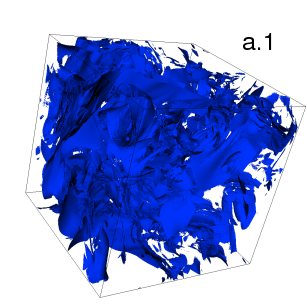
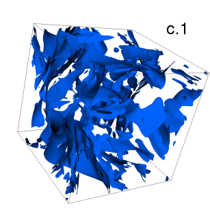
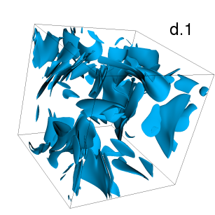
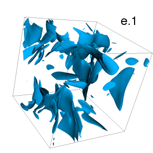
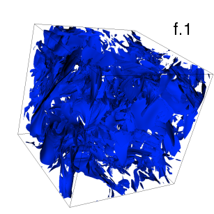
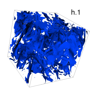
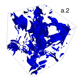
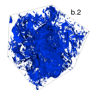
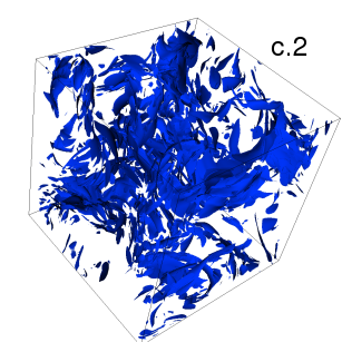
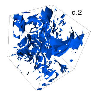
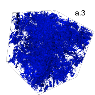
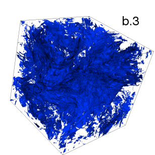
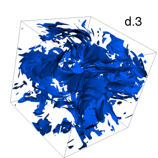
Figure 28: Isosurfaces of the local fluid energy dissipation rate $\epsilon_{u}$: (a.1) ${\rm Pr_{M}}=0.1$ (R1), (b.1) ${\rm Pr_{M}}=0.5$ (R2), (c.1) ${\rm Pr_{M}}=1.0$ (R3), (d.1) ${\rm Pr_{M}}=5.0$ (R4), (e.1) ${\rm Pr_{M}}=10.0$ (R5), (f.1) ${\rm Pr_{M}}=1.0$ (R3B), (g.1) ${\rm Pr_{M}}=5.0$ (R4B), (h.1) ${\rm Pr_{M}}=10.0$ (R5B), (a.2) ${\rm Pr_{M}}=0.01$ (R1C), (b.2) ${\rm Pr_{M}}=0.1$ (R2C), (c.2) ${\rm Pr_{M}}=1.0$ (R3C), and (d.2) ${\rm Pr_{M}}=10.0$ (R4C) for decaying MHD turbulence; and for statistically steady MHD turbulence (a.3) ${\rm Pr_{M}}=0.01$ (R1D), (b.3) ${\rm Pr_{M}}=0.1$ (R2D), (c.3) ${\rm Pr_{M}}=1.0$ (R3D), and (d.3) ${\rm Pr_{M}}=10.0$ (R4D); these isosurfaces go through points at which the value of $\epsilon_{u}$ is two standard deviations above its mean value (for any given plot).

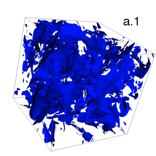
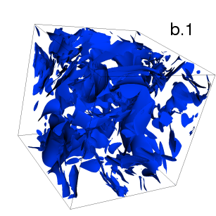
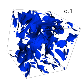
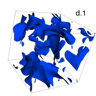
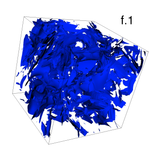
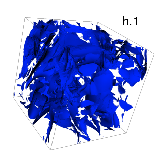
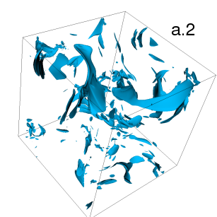
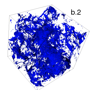
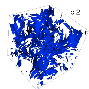
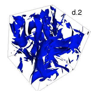
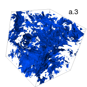
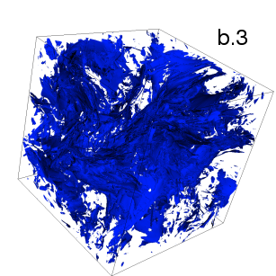
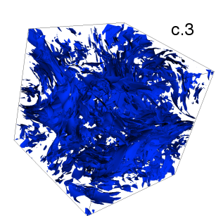
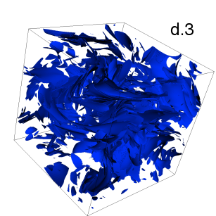
Figure 29: Isosurfaces of the local magnetic-energy dissipation rate $\epsilon_{b}$: (a.1) ${\rm Pr_{M}}=0.1$ (R1), (b.1) ${\rm Pr_{M}}=0.5$ (R2), (c.1) ${\rm Pr_{M}}=1.0$ (R3), (d.1) ${\rm Pr_{M}}=5.0$ (R4), (e.1) ${\rm Pr_{M}}=10.0$ (R5), (f.1) ${\rm Pr_{M}}=1.0$ (R3B), (g.1) ${\rm Pr_{M}}=5.0$ (R4B), and (h.1) ${\rm Pr_{M}}=10.0$ (R5B). (a.2) ${\rm Pr_{M}}=0.01$ (R1C), (b.2) ${\rm Pr_{M}}=0.1$ (R2C), (c.2) ${\rm Pr_{M}}=1.0$ (R3C), and (d.2) ${\rm Pr_{M}}=10.0$ (R4C) for decaying MHD turbulence; and for statistically steady MHD turbulence (a.3) ${\rm Pr_{M}}=0.01$ (R1D), (b.3) ${\rm Pr_{M}}=0.1$ (R2D), (c.3) ${\rm Pr_{M}}=1.0$ (R3D), and (d.3) ${\rm Pr_{M}}=10.0$ (R4D); these isosurfaces go through points at which the value of $\epsilon_{b}$ is two standard deviations above its mean value (for any given plot).

Isosurfaces of $\epsilon_{u}$ are shown at $t_{c}$ for runs R1-R5 in Figs. 28(a.1)-28(e.1), runs R3B-R5B in Figs. 28(f.1)-28(h.1), and runs R1C-R4C in Figs. 28(a.2)-28(d.2) for decaying MHD turbulence; and for statistically steady MHD turbulence they are shown in Figs. 28(a.3)-28(d.3) for runs R1D-R4D; the isosurfaces go through points at which the value of $\epsilon_{u}$ is two standard deviations above its mean value (for any given plot). Similar isosurfaces of $\epsilon_{b}$ are shown at $t_{c}$ for runs R1-R5 in Figs. 29(a.1)-29(e.1), runs R3B-R5B in Figs. 29(f.1)-29(h.1), and runs R1C-R4C in Figs. 29(a.2)-29(d.2) for decaying MHD turbulence; and for statistically steady MHD turbulence they are shown in Figs. 29(a.3)-29(d.3) for runs R1D-R4D; the isosurfaces go through points at which the value of $\epsilon_{b}$ is two standard deviations above its mean value (for any given plot). Here too the isosurfaces are sheets; they lie close to, but are not coincident with, isosurfaces of $\omega$ and $j$; changes in ${\rm Pr_{M}}$ affect these isosurfaces much as they affect isosurfaces of $\omega$ and $j$.

Isosurfaces of $\bar{p}$ are shown at $t_{c}$ for runs R1-R5 in Figs. 30(a.1)-30(e.1) and runs R3B-R5B in Figs. 30(f.1)-30(h.1) for decaying MHD turbulence; and for statistically steady MHD turbulence they are shown in Figs. 30(a.3)-30(d.3) for runs R1D-R4D; the isosurfaces go through points at which the value of $\bar{p}$ is two standard deviations above its mean value (for any given plot). The general form of these isosurfaces is cloud-type, to borrow the term that has been used for isosurfaces of the pressure in fluid turbulence [60]. Here also changes in ${\rm Pr_{M}}$ affect these isosurfaces much as they affect isosurfaces of $\omega$ and $j$, in as much as high-intensity isosurfaces are suppressed as ${\rm Pr_{M}}$ increases via an increase in $\nu$, unless this is compensated for by an increase in the initial energy (in the case of decaying MHD turbulence) or ${\rm Re}_{\lambda}$.

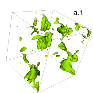
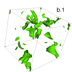
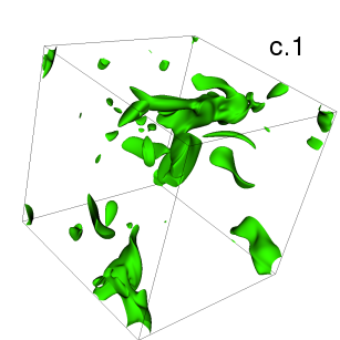
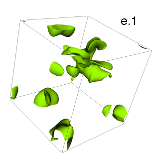
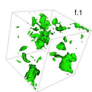
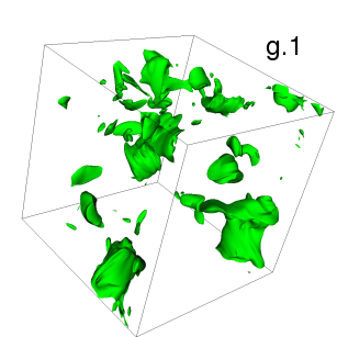
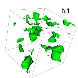
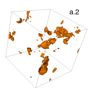
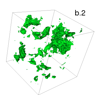
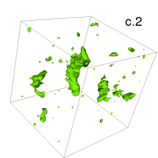
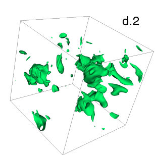
Figure 30: Isosurfaces of the local effective pressure $\bar{p}$: (a.1) ${\rm Pr_{M}}=0.1$ (R1), (b.1) ${\rm Pr_{M}}=0.5$ (R2), (c.1) ${\rm Pr_{M}}=1.0$ (R3), (d.1) ${\rm Pr_{M}}=5.0$ (R4), (e.1) ${\rm Pr_{M}}=10.0$ (R5), (f.1) ${\rm Pr_{M}}=1.0$ (R3B), (g.1) ${\rm Pr_{M}}=5.0$ (R4B), and (h.1) ${\rm Pr_{M}}=10.0$ (R5B) for decaying MHD turbulence; and for statistically steady MHD turbulencs (a.2) ${\rm Pr_{M}}=0.01$ (R1D), (b.2) ${\rm Pr_{M}}=0.1$ (R2D), (c.2) ${\rm Pr_{M}}=1.0$ (R3D), and (d.2) ${\rm Pr_{M}}=10.0$ (R4D); these isosurfaces go through points at which the value of $\bar{p}$ is two standard deviations above its mean value (for any given plot).

3.7 Joint probability distribution functions

In this Subsection we present three sets of joint PDFs that have, to the best of our knowledge, not been used to characterise MHD turbulence. The first of these is a $QR$ plot that is often used in studies of fluid turbulence as we have discussed in Subsections 2.2 and 3.1; the next is a joint PDF of $\omega$ and $j$; and the last is a joint PDF of $\epsilon_{u}$ and $\epsilon_{b}$.

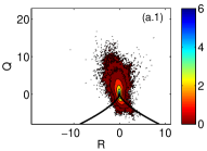
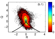
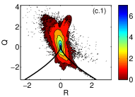
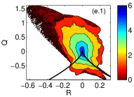
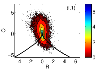
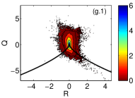
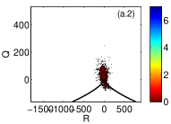
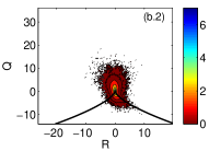
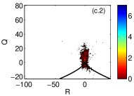
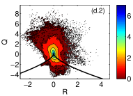
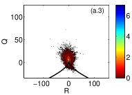
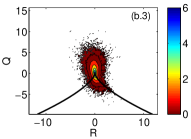
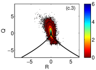
Figure 31: $QR$ plots, i.e., joint PDFs of $Q$ and $R$ shown as filled contour plots on a logarithmic scale for (a.1) ${\rm Pr_{M}}=0.1$ (R1), (b.1) ${\rm Pr_{M}}=0.5$ (R2), (c.1) ${\rm Pr_{M}}=1.0$ (R3), (d.1) ${\rm Pr_{M}}=5.0$ (R4), (e.1) ${\rm Pr_{M}}=10.0$ (R5), (f.1) ${\rm Pr_{M}}=1.0$ (R3B), (g.1) ${\rm Pr_{M}}=5.0$ (R4B), (h.1) ${\rm Pr_{M}}=10.0$ (R5B), (a.2) ${\rm Pr_{M}}=0.01$ (R1C), (b.2) ${\rm Pr_{M}}=0.1$ (R2C), (c.2) ${\rm Pr_{M}}=1.0$ (R3C), and (d.2) ${\rm Pr_{M}}=10.0$ (R4C) for decaying MHD turbulence; and for statistically steady MHD turbulence (a.3) ${\rm Pr_{M}}=0.01$ (R1D), (b.3) ${\rm Pr_{M}}=0.1$ (R2D), (c.3) ${\rm Pr_{M}}=1.0$ (R3D), and (d.3) ${\rm Pr_{M}}=10.0$ (R4D). The arguments $Q$ and $R$ of the $QR$ plots are normalised by $\langle\omega^{2}\rangle$ and $\langle\omega^{2}\rangle^{3/2}$, respectively. The black curve is the zero-discriminant line $D\equiv\frac{27}{4}R^{2}+Q^{3}=0$.

We show $QR$ plots, i.e., joint PDFs of $Q$ and $R$, via filled contour plots; these are obtained at $t_{c}$ for runs R1-R5 in Figs. 31(a.1)-31(e.1), runs R3B-R5B in Figs. 31(f.1)-31(h.1), and runs R1C-R4C in Figs. 31(a.2)-31(d.2) for decaying MHD turbulence; and for statistically steady MHD turbulence they are shown in Figs. 31(a.3)-31(d.3) for runs R1D-R4D; the black curve in these plots is the zero-discriminant line $D\equiv\frac{27}{4}R^{2}+Q^{3}=0$. These $QR$ plots retain overall, aside from some distortions, the characteristic tear-drop structure familiar from fluid turbulence (see Subsection 3.1 and Fig. 5). If we recall our discussion of $QR$ plots in Subsection 2.2 and we notice that, as we increase ${\rm Pr_{M}}$ [Figs. 31(a.1)-31(e.1) for runs R1-R5, respectively] while holding $\eta$ and the initial energy fixed, there is a general decrease in the probability of having large values of $Q$ and $R$, i.e., regions of large strain or vorticity are suppressed; this corroborates what we have found from the PDFs and isosurfaces discussed above. However, if we compensate for the increase in $\nu$ by increasing the initial energy, or ${\rm Re}_{\lambda}$, so that $k_{\rm max}\eta_{d}^{u}$ and $k_{\rm max}\eta_{d}^{b}$ are both $\simeq 1$, we see that $Q$ and $R$ can increase again. Note that when ${\rm Pr_{M}}$ is very small as in run R1D [Fig. 31(a.3)], the tear-drop structure is very much like its fluid-turbulence counterpart Fig. 5, which might well correlate with the appearance of some tube-type structures in the $\omega$ isosurface in enlarged versions of Fig. 26(a.3).

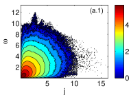
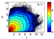
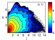
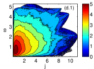
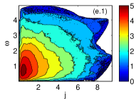
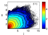
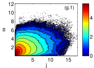
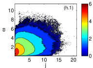
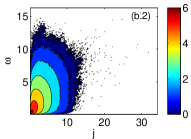
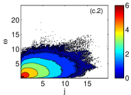
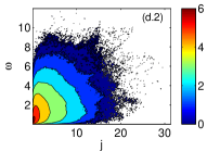
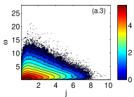
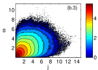
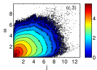
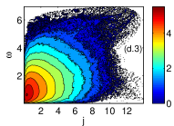
Figure 32: Joint PDFs of $\omega$ and $j$ shown as filled contour plots on a logarithmic scale for (a.1) ${\rm Pr_{M}}=0.1$ (R1), (b.1) ${\rm Pr_{M}}=0.5$ (R2), (c.1) ${\rm Pr_{M}}=1.0$ (R3), (d.1) ${\rm Pr_{M}}=5.0$ (R4), (e.1) ${\rm Pr_{M}}=10.0$ (R5), (f.1) ${\rm Pr_{M}}=1.0$ (R3B), (g.1) ${\rm Pr_{M}}=5.0$ (R4B), (h.1) ${\rm Pr_{M}}=10.0$ (R5B), (a.2) ${\rm Pr_{M}}=0.01$ (R1C), (b.2) ${\rm Pr_{M}}=0.1$ (R2C), (c.2) ${\rm Pr_{M}}=1.0$ (R3C), and (d.2) ${\rm Pr_{M}}=10.0$ (R4C) for decaying MHD turbulence; and for statistically steady MHD turbulence (a.3) ${\rm Pr_{M}}=0.01$ (R1D), (b.3) ${\rm Pr_{M}}=0.1$ (R2D), (c.3) ${\rm Pr_{M}}=1.0$ (R3D), and (d.3) ${\rm Pr_{M}}=10.0$ (R4D). The arguments of the joint PDFs are normalised by their standard deviations.

We now consider joint PDFs of $\omega$ and $j$ that are obtained at $t_{c}$ for runs R1-R5 in Figs. 32(a.1)-32(e.1), runs R3B-R5B in Figs. 32(f.1)-32(h.1), and runs R1C-R4C in Figs. 32(a.2)-32(d.2) for decaying MHD turbulence; and for statistically steady MHD turbulence they are shown in Figs. 32(a.3)-32(d.3) for runs R1D-R4D. All these joint PDFs have long tails; as we move away from ${\rm Pr_{M}}=1$ they become more and more asymmetrical. Furthermore, as we expect, the tails of these PDFs are drawn in towards small values of $\omega$ and $j$ as we increase ${\rm Pr_{M}}$ [Figs. 32(a.1)-32(e.1) for runs R1-R5, respectively] while holding $\eta$ and the initial energy fixed. However, if we compensate for the increase in $\nu$ by increasing the initial energy or ${\rm Re}_{\lambda}$, so that $k_{\rm max}\eta_{d}^{u}$ and $k_{\rm max}\eta_{d}^{b}$ are both $\simeq 1$, we see that the tails of the PDFs get elongated again.

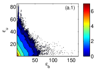
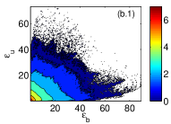
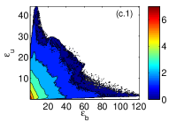
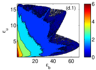
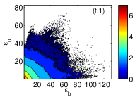
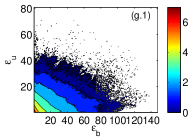
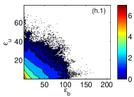
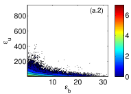
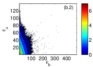
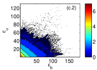
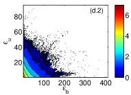
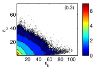
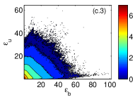
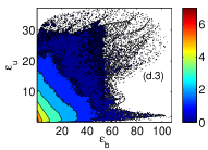
Figure 33: Joint PDFs of $\epsilon_{u}$ and $\epsilon_{b}$ shown as filled contour plots on a logarithmic scale for (a.1) ${\rm Pr_{M}}=0.1$ (R1), (b.1) ${\rm Pr_{M}}=0.5$ (R2), (c.1) ${\rm Pr_{M}}=1.0$ (R3), (d.1) ${\rm Pr_{M}}=5.0$ (R4), (e.1) ${\rm Pr_{M}}=10.0$ (R5), (f.1) ${\rm Pr_{M}}=1.0$ (R3B), (g.1) ${\rm Pr_{M}}=5.0$ (R4B), (h.1) ${\rm Pr_{M}}=10.0$ (R5B), (a.2) ${\rm Pr_{M}}=0.01$ (R1C), (b.2) ${\rm Pr_{M}}=0.1$ (R2C), (c.2) ${\rm Pr_{M}}=1.0$ (R3C), and (d.2) ${\rm Pr_{M}}=10.0$ (R4C) for decaying MHD turbulence; and for statistically steady MHD turbulence (a.3) ${\rm Pr_{M}}=0.01$ (R1D), (b.3) ${\rm Pr_{M}}=0.1$ (R2D), (c.3) ${\rm Pr_{M}}=1.0$ (R3D), and (d.3) ${\rm Pr_{M}}=10.0$ (R4D). The arguments of the joint PDFs are normalised by their standard deviations.

In the end we consider joint PDFs of $\epsilon_{u}$ and $\epsilon_{b}$ that are obtained at $t_{c}$ for runs R1-R5 in Figs. 33(a.1)-33(e.1), runs R3B-R5B in Figs. 33(f.1)-33(h.1), and runs R1C-R4C in Figs. 33(a.2)-33(d.2) for decaying MHD turbulence; and for statistically steady MHD turbulence they are shown in Figs. 33(a.3)-33(d.3) for runs R1D-R4D. The trends here are similar to the ones discussed in the previous paragraph. In particular, these joint PDFs have long tails; as we move away from ${\rm Pr_{M}}=1$ they become more and more asymmetrical; and the tails of these PDFs are drawn in towards small values of $\epsilon_{u}$ and $\epsilon_{b}$ as we increase ${\rm Pr_{M}}$ [Figs. 33(a.1)-33(e.1) for runs R1-R5, respectively] while holding $\eta$ and the initial energy fixed. But, if we make up for the increase in $\nu$ by increasing the initial energy or ${\rm Re}_{\lambda}$ so that $k_{\rm max}\eta_{d}^{u}$ and $k_{\rm max}\eta_{d}^{b}$ are both $\simeq 1$, we see that the tails of the PDFs get elongated again.

4 Discussions and Conclusion

We have carried out an extensive study of the statistical properties of both decaying and statistically steady homogeneous, isotropic MHD turbulence. Our study, which has been designed specifically to study the systematics of the dependence of these properties on the magnetic Prandtl number ${\rm Pr_{M}}$, uses a large number of statistical measures to characterise the statistical properties of both decaying and statistically steady MHD turbulence. Our study is restricted to incompressible MHD turbulence; we do not include a mean magnetic field as, e.g., in Refs. [33]; furthermore we do not study Lagrangian properties considered, e.g., in Ref. [34]. In our studies we obtain (a) various PDFs, such as those of the moduli of the vorticity and current density, the energy dissipation rates, of cosines of angles between various vectors, and scale-dependent velocity and magnetic-field increments, (b) spectra, e.g., those of the energy and the effective pressure, (c) velocity and magnetic-field structure functions that can be used to characterise intermittency, (d) isosurfaces of quantities such as the moduli of the vorticity and current, and (e) joint PDFs such as $QR$ plots. The evolution of these properties with ${\rm Pr_{M}}$ has been described in detail in the previous Section.

To the best of our knowledge, such a comprehensive study of the ${\rm Pr_{M}}-$dependence of incompressible, homogeneous, isotropic MHD turbulence, both decaying and statistically steady, has not been attempted before. Studies that draw their inspiration from astrophysics often consider anisotropic flows [76, 77, 78, 79, 80, 81, 82, 83], flows that are compressible [35, 84], or flows that include a mean magnetic field [33, 81, 85, 86]. Yet other studies concentrate on the alignment between various vectors such as ${\bf u}$ and ${\bf b}$ as, e.g., in Refs. [28, 35, 52]; some of these include a few, but not all, of the PDFs we have studied; and, typically, these studies are restricted to the case ${\rm Pr_{M}}=1$. Some of the spectra we study have been obtained in earlier DNS studies but, typically, only for the case ${\rm Pr_{M}}=1$; a notable exception is Ref. [37], which examines the ${\rm Pr_{M}}-$dependence of energy spectra but with a relatively low resolution. References [6, 32, 87] have also considered some ${\rm Pr_{M}}-$dependence but not for low ${\rm Pr_{M}}$. Isosurfaces of the moduli of the vorticity and current density have been obtained earlier [25, 38, 74] for the case ${\rm Pr_{M}}=1$. The ${\rm Pr_{M}}$ dependence of these and other isosurfaces is presented here for the first time. The joint PDFs we have shown above have also not been investigated before.

Here we wish to highlight, and examine in detail, the implications of our study for intermittency. Some earlier DNS studies, such as Refs. [30], had noted that, for the case ${\rm Pr_{M}}=1$, the magnetic field is more intermittent than the velocity field. This is why we have concentrated on velocity and magnetic-field structure functions. Our study confirms this finding, for the case ${\rm Pr_{M}}=1$. This can be seen clearly from the comparison of our exponent ratios, for ${\rm Pr_{M}}=1$, with those of the recent DNS of decaying-MHD-turbulence in Ref. [30] in Table 8; the errorbars that we quote for our exponent ratios have been calculated as described in the previous Section; we have obtained exponent ratios for Ref. [30] by digitising [89] the data in their plot [Fig. 3 of Ref. [30]] of multiscaling exponents versus the order $p$ (error bars are not given in their plot). Thus, at least given our errorbars, there is agreement between our exponent ratios, both for decaying and statistically steady MHD turbulence, and those of Ref. [30] for ${\rm Pr_{M}}=1$. We note in passing that the latter DNS is one of decaying MHD turbulence but with a very special initial condition, which allows an effective resolution greater than that we have obtained; however, the initial condition we use in our decaying-MHD-turbulence DNS is more generic than that of Ref. [30]. It is our expectation that nonuniversal effects, associated with different initial conditions [26, 49], might not affect multiscaling exponent ratios, except if we use nongeneric, power-law initial conditions [26] in which $E(k)$ grows with $k$ (at least until some large-$k$ cutoff).

Direct numerical simulations of decaying-MHD-turbulence, e.g., those of Refs. [25, 30], often average data obtained from field configurations at different times that are close to the time at which the peak appears in plots of the energy-dissipation rate. This is a reasonable procedure, for ${\rm Pr_{M}}=1$, because the temporal evolution of the system is slow in the vicinity of this peak. We have not adopted this procedure here because, as we move away from ${\rm Pr_{M}}=1$, the cascade-completion peaks occur at different times in plots of $\epsilon_{u}$ and $\epsilon_{b}$ as we have discussed in detail in earlier sections of this paper.

Let us now turn to the ${\rm Pr_{M}}-$dependence of the multiscaling exponent ratios shown in Tables 6 and 7 and in Figs.24(a.3)-24(d.3) and 25(a.3)-25(d.3). Even though our error bars are large, given the conservative, local-slope error analysis we have described in the previous Section, a trend emerges: at large values of ${\rm Pr_{M}}$ the magnetic field is clearly more intermittent than the velocity field, in as much as the deviations of $\zeta_{p}^{b}$ from the simple-scaling prediction are stronger than their counterparts for $\zeta_{p}^{u}$. However, the velocity field becomes more intermittent than the magnetic field as we lower ${\rm Pr_{M}}$. Could this result, namely, the dependence of our multiscaling exponent ratios on ${\rm Pr_{M}}$, be an artifact? We believe not. As we have discussed above, dissipation ranges in our spectra are adequately resolved; furthermore, we have determined exponent ratios from a a rather stringent local-slope analysis, which is rarely presented in earlier DNS studies of MHD turbulence. Ultimately, of course, this ${\rm Pr_{M}}$ dependence of multiscaling exponents in MHD turbulence must be tested in detail in very-high-resolution DNS studies of MHD turbulence; such studies should become possible with the next generation of supercomputers.

It is useful to note at this stage that a recent experimental study of MHD turbulence in the solar wind [56] provides evidence for velocity fields that are more strongly intermittent than the magnetic field; this study does not give the value of ${\rm Pr_{M}}$. However, their data for multiscaling exponents are qualitatively similar to those we obtain at low values of ${\rm Pr_{M}}$. Furthermore, PDFs of $H_{C}$ have also been obtained from solar-wind data [55]; these are similar to the PDFs we obtain for $H_{C}$. Of course, we must exercise caution in comparing results from DNS studies of homogeneous, isotropic, incompressible MHD turbulence with measurements on the solar wind where anisotropy and compressibility can be significant; and, for the solar wind, we might also have to consider kinetic effects that are not captured by the MHD equations.

The last point we wish to address is the issue of strong universality of exponent ratios. In the fluid-turbulence context such strong universality [41, 42] implies the equality of exponents (and, therefore, their ratios) determined from decaying-turbulence studies (say at the cascade-completion time) or from studies of statistically steady turbulence. Does such strong universality have an analogue in MHD turbulence? Our data, for any fixed value of ${\rm Pr_{M}}$ in Tables 6 and 7, are consistent with such strong universality of multiscaling exponent ratios in MHD turbulence; but, of course, our large errorbars imply that a definitive confirmation of such strong universality in MHD turbulence must await DNS studies that might become possible in the next generation of high-performance-computing facilities.

References

References

- [1] A. R. Choudhuri, The Physics of Fluids and Plasmas: An Introduction for Astrophysicists (Cambridge University Press, Cambridge, UK, 1998).
- [2] V. Krishan, Astrophysical Plasmas and Fluids (Kluwer Academic Publishers, Netherlands, 1999).
- [3] G. Rüdiger and R. Hollerbach, The Magnetic Universe: Geophysical and Astrophysical Dynamo Theory (Wieley, Weinheim, 2004).
- [4] H. Goedbloed and S. Poedts, Principles of Magnetohydrodynamics With Applications to Laboratory and Astrophysical Plasmas (Cambridge University Press, Cambridge, UK, 2004).
- [5] D. Biskamp, Magnetohydrodynamic Turbulence (Cambridge University Press, Cambridge, UK, 2003).
- [6] A.A. Schekochihin et al., New J. Phys. 4, 84 (2002); New J. Phys. 9, 300 (2007);
- [7] M.K. Verma, Phys. Rep. 401, 229 (2004).
- [8] B. G. Elmegreen and J. Scalo, Annual Rev. of Astronomy and Astrophys. 42, 211 (2004).
- [9] Focus on Magnetohydrodynamics and the Dynamo Problem, New J. Phys. 9, (2007).
- [10] E. Dormy and J.-L. Le Mouël, C.R. Physique 9 (2008).
- [11] G. Sahoo, D. Mitra, and R. Pandit, Phys. Rev. E 81, 036317 (2010).
- [12] B. Lehnert, Q. Appl. Math. 12, 321 (1955).
- [13] P. H. Roberts and G. A. Glatzmaier, Rev. Mod. Phys. 72, 1081 (2000).
- [14] N. L. Peffley, A. B. Cawthorne, and D. P. Lathrop, Phys. Rev. E 61, 5287 (2000); W.L. Shew and D.P. Lathrop, Phys. Earth Planet. Inter. 153, 136 (2005).
- [15] A. Gailitis et al., Phys. Rev. Lett. 84, 4365 (2000); Phys. Rev. Lett. 86, 3024 (2001); Rev. Mod. Phys. 74, 973 (2002); Surv. Geophys. 24, 247 (2003); Phys. Plasmas 11, 2838 (2004).
- [16] R. Stieglitz and U. Müller, Phys. Fluids 13, 561 (2001); U. Müller and R. Stieglitz, Nonlin. Proc. Geophys. 9, 165 (2002); U. Müller, R. Stieglitz, and S. Horanyi, J. Fluid Mech. 498, 31 (2004).
- [17] F. Pétrélis and S. Fauve, Europhys. Lett. 22, 273 (2001); 76, 602 (2006); S. Fauve and F. Pétrélis, in Peyresq Lectures on Nonlinear Phenomena, edited by J.-A. Sepulchre (World Scientific, Singapore, 2003), Vol. 2, pp. 1–64; S. Fauve and F. Pétrélis, C.R. Physique 8, 87 (2007).
- [18] M. Bourgoin et al., Phys. Fluids 14, 3046 (2002); R. Monchaux et al., Phys. Rev. Lett. 98, 044502 (2007).
- [19] M. Bourgoin et al., Phys. Fluids 14, 3046 (2002); 16, 2529 (2004); L. Marié et al., Magnetohydrodynamics 38, 163 (2002); R. Monchaux et al., Phys. Rev. Lett. 98, 044502 (2007).
- [20] Y. Ponty, P. D. Mininni, D. C. Montgomery, J.-F. Pinton, H. Politano, and A. Pouquet, Phys. Rev. Lett. 94, 164502 (2005).
- [21] S. Boldyrev, Phys. Rev. Lett. 96, 115002 (2006); S. Boldyrev, J. Mason, and F. Cattaneo, Astrophys. J. 699 L39 (2009).
- [22] A.A. Schekochihin et al., Phys. Rev. Lett. 92, 054502 (2004).
- [23] A. N. Kolmogorov, Dokl. Akad. Nauk. SSSR 30, 9 (1941); 32, 16 (1941); Proc. R. Soc. London, Ser. A 434, 9 (1991); 434, 15 (1991); C. R. Acad. Sci. USSR 30, 301 (1941).
- [24] U. Frisch, Turbulence: The Legacy of A. N. Kolmogorov (Cambridge University, Cambridge, England, 1996).
- [25] W-C. Müller and D. Biskamp, Phys. Rev. Lett. 84, 475 (2000); Phys. Rev. E 67, 066302 (2003); D. Biskamp and W-C. Müller, Phys of Plasmas 7, 4889 (2000).
- [26] C. Kalelkar and R. Pandit, Phys. Rev. E 69, 046304 (2004).
- [27] P. D. Mininni, A. G. Pouquet, and D. C. Montgomery, Phys. Rev. Lett. 97, 244503 (2006).
- [28] J. Mason, F. Cattaneo, and S. Boldyrev, Phys. Rev. E 77, 036403 (2008).
- [29] J. Baerenzung, H. Politano, Y. Ponty, and A. Pouquet, Phys. Rev. E 77, 046303 (2008); 78, 026310 (2008).
- [30] P. D. Mininni and A. Pouquet, Phys. Rev. E 80, 025401 (2009).
- [31] Y. Ponty, J. P. Laval, B. Dubrulle, F. Daviaud, and J.-F. Pinton, Phys. Rev. Lett. 99, 224501 (2007); C. R. Acad. Sci. (Paris) 9, 749 (2008).
- [32] A. Brandenburg, Astrophys. J. 697, 1206 (2009).
- [33] P. Goldreich and S. Sridhar, Astrophys. J. 438, 763 (1995).
- [34] For representative Lagrangian studies of MHD turbulence see H. Homann, R. Grauer, A. Busse and W. C. Mul̈ler, J. Plasma Phys. 73, 821 (2007).
- [35] A. Brandenburg, A. Nordlund, R. F. Stein, and U. Torkelsson, Astrophys. J. 446, 741 (1995); A. Brandenburg, Chaos, Solitons and Fractals 5, 2023 (1995).
- [36] N. Cao, S. Chen, and G. D. Doolen, Phys. Fluids 11, 2235 (1999).
- [37] H. Chou, Astrophys. J. 556, 1038 (2001).
- [38] P. D. Mininni and A. Pouquet, Phys. Rev. Lett. 99, 254502 (2007).
- [39] R. Benzi, S. Ciliberto, R. Tripiccione, C. Baudet, F. Massaioli, and S. Succi, Phys. Rev. E 48, R29 (1993).
- [40] S. Chakraborty, U. Frisch, and S. S. Ray, J. Fluid Mech., 649, 275 (2010).
- [41] V. S. L’vov, R. A. Pasmanter, A. Pomyalov, and I. Procaccia, Phys. Rev. E 67, 066310 (2003).
- [42] S. S. Ray, D. Mitra, and R. Pandit, New J. Phys. 10, 033003 (2008).
- [43] C. Canuto, M.Y. Hussaini, A. Quarteroni and T.A. Zang, Spectral Methods in Fluid Dynamics (Springer, Berlin, 1988); Spectral Methods Evolution to Complex Geometries and Applications to Fluid Dynamics (Springer, Berlin, 2007).
- [44] R. Courant, K. Friedrichs, and H. Lewy, IBM Journal 11, 215 (1967). (English translation of the original work, ”Ub̈er die Partiellen Differenzengleichungen der Mathematischen Physik,” Math. Ann. 100, 32 (1928).
- [45] C. Kalelkar, Phys. Rev. E 72, 056307 (2005).
- [46] C. Kalelkar, Phys. Rev. E 73, 046301 (2006).
- [47] C. Kalelkar, R. Govindarajan, and R. Pandit, Phys. Rev. E 72, 017301 (2005).
- [48] P. Perlekar, D. Mitra and R. Pandit, Phys. Rev. Lett. 97, 264501 (2006).
- [49] E. Lee, M. E. Brachet, A. Pouquet, P. D. Mininni, and D. Rosenberg, Phys. Rev. E 81, 016318 (2010).
- [50] A.G. Lamorgese, D.A. Caughey, and S.B. Pope, Phys. Fluids 17, 015106 (2005).
- [51] T. Stribling and W. H. Matthaeus, Phys. Fluids B 2, 1979 (1990).
- [52] W. H. Matthaeus, A. Pouquet, P. D. Mininni, P. Dmitruk, and B. Breech, Phys. Rev. Lett. 100, 085003 (2008).
- [53] M. Wan, S. Oughton, S. Servidio, and W. H. Matthaeus, Phys. Plasmas 16, 080703 (2009).
- [54] W. H. Matthaeus and M. L. Goldstein, J. Geophys. Res. 87, 6011 (1982).
- [55] J. J. Podesta, D. A. Roberts, and M. L. Goldstein, Astrophys. J. 664, 543 (2007); J. J. Podesta, B. D. G. Chandran, A. Bhattacharjee, D. A. Roberts and M. L. Goldstein, J. Geophys. Res., 114, A01107 (2009).
- [56] C. Salem, A. Mangeney, S. D. Bale, and P. Veltri, Astrophys. J. 702, 537 (2009).
- [57] P.A. Davidson, Turbulence (Oxford University Press, Oxford, 2004).
- [58] B. J. Cantwell, Phys. Fluids A 5, 2008 (1993).
- [59] L. Biferale, L. Chevillard, C. Meneveau, and F. Toschi, Phys. Rev. Lett. 98, 214501 (2007).
- [60] U. Schumann and G. S. Patterson, J. Fluid Mech. 88, 685 (1978).
- [61] S. Chen, G. Doolen, J. R. Herring, R. H. Kraichnan, S. A. Orszag, and Z. S. She, Phys. Rev. Lett. 70, 3051 (1993).
- [62] T. Gotoh, D. Fukayama, and T. Nakano, Phys. Fluids 14, 1065 (2002).
- [63] Y. Kaneda, T. Ishihara, M. Yokokawa, K. Itakura, and A. Uno, Phys. Fluids 15, L21 (2003).
- [64] J. Schumacher, K. R. Sreenivasan, and V. Yakhot, New J. Phys. 9, 89 (2007); J. Schumacher, Europhys. Lett. 80, 54001 (2007).
- [65] R. Pandit, P. Perlekar, S.S. Ray, Pramana 73, 157 (2009).
- [66] J. Schumacher, B. Eckhardt and C. R. Doering, Phys. Lett. A 374, 861 (2010).
- [67] T. Gotoh and D. Fukayama, Phys. Rev. Lett. 86, 3775 (2001).
- [68] E. Kit, A. Tsinober, J.L. Balint, J.M. Wallace, and E. Levich, Phys. Fluids 30, 3323 (1987).
- [69] G. Pedrizzetti, E. A. Novikov, A. A. Praskovsky Phys. Rev. E 53, 475 (1996).
- [70] S. Jung and H. L. Swinney, Phys. Rev. E 72, 026304 (2005).
- [71] N. Okamoto, K. Yoshimatsu, K. Schneider, M. Farge, and Y. Kaneda, Phys. Fluids 19, 115109 (2007).
- [72] J. M. Weygand et al., J. Geophys. Res. 110, A01205 (2005).
- [73] P. Iroshnikov, Astron. Zh. 40, 742 (1963); R. H. Kraichnan, Phys. Fluids 8, 1385 (1965).
- [74] K. Yoshimatsu, Y. Kondo, K. Schneider, N. Okamoto, H. Hagiwara, and M. Farge, Phys. Plasmas 16, 082306 (2009).
- [75] R. Grauer and C. Marliani, Phys. Rev. Lett. 84, 4850 (2000).
- [76] D. Montgomery and L. Turner, Phys. Fluids 24, 825 (1981).
- [77] P. Veltri, A. Mangeney, and M. Dobrowolny, Nuovo Cimento B 68, 235 (1982).
- [78] R. M. Kinney and J. C. McWilliams, J. Plasma Phys. 57, 73 (1997); Phys. Rev. E 57, 7111 (1998).
- [79] S. Galtier, A. Pouquet, and A. Mangeney, Phys. Plasmas 12, 092310 (2005).
- [80] B. D. G. Chandran, Astrophys. J. 685, 646 (2008).
- [81] J. Shebalin, W. H. Matthaeus, and D. Montgomery, J. Plasma Phys. 29, 525 (1983).
- [82] A. Brandenburg, K. Subramanian, Astronomische Nachrichten 328, 507-512 (2007).
- [83] B. Bigot, S. Galtier, and H. Politano, Phys. Rev. Lett. 100, 074502 (2008)
- [84] M. Christensson, M. Hindmarsh and A. Brandenburg, Phys. Rev. E 64, 056405 (2001).
- [85] A. Alemany, R. Moreau, P.-L. Sulem, and U. Frisch, J. Mech. 18, 277 (1979); M. Garnier, A. Alemany, P.-L. Sulem, and A. Pouquet, J. Mec. 20, 233 (1981).
- [86] S. Oughton, E. R. Priest, and W. H. Matthaeus, J. Fluid Mech. 280, 95 (1994).
- [87] A. B. Iskakov, A. A. Schekochihin, S. C. Cowley, J. C. McWilliams, and M. R. E. Proctor, Phys. Rev. Lett. 98, 208501 (2007).
- [88] A. Basu, A. Sain, S.K. Dhar and R. Pandit, Phys. Rev. Lett. 81, 2687 (1998).
- [89] For digitising we use the software G3DATA (http://www.frantz.fi/software/g3data.php) available in the Ubuntu repositories.