On building and fitting a spatio-temporal change-point model for settlement and growth at Bourewa, Fiji Islands

Abstract

The Bourewa beach site on the Rove Peninsula of Viti Levu is the earliest known human settlement in the Fiji Islands. How did the settlement at Bourewa develop in space and time? We have radiocarbon dates on sixty specimens, found in association with evidence for human presence, taken from pits across the site. Owing to the lack of diagnostic stratigraphy, there is no direct archaeological evidence for distinct phases of occupation through the period of interest. We give a spatio-temporal analysis of settlement at Bourewa in which the deposition rate for dated specimens plays an important role. Spatio-temporal mapping of radiocarbon date intensity is confounded by uneven post-depositional thinning. We assume that the confounding processes act in such a way that the absence of dates remains informative of zero rate for the original deposition process. We model and fit the onset-field, that is, we estimate for each location across the site the time at which deposition of datable specimens began. The temporal process generating our spatial onset-field is a model of the original settlement dynamics.

1 Introduction

Bourewa beach is an archaeological site on the southwest coast of Viti Levu, the largest island in the Fiji Islands Group. It was identified in Nunn et al. (2004) as a site of likely early settlement by surface finds of distinctive early Lapita-era ceramics. In the course of the excavation, which ended in February 2009, in excess of one hundred pits, of varying sizes, were dug. Material was selected from some of these pits for radiocarbon dating. These data, and their observation model, are described in Section 3. The likelihoods for the unknown ages of the specimens are plotted in Fig. 1.

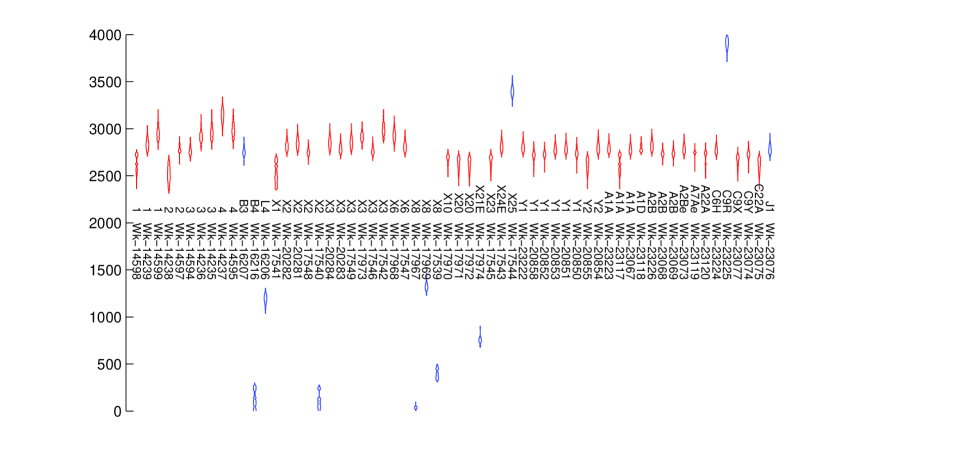
Figure 1: All Bourewa data: (y-axis) years BP, (x-axis) specimen index, likelihoods (blue) data omitted from study, (red) data retained. Two early dates were ajudged insecurely linked to evidence for human presence, and the later dates belong to a qualitatively different phase of activity at the site. Text (top row) is pit-name and (bottom row) date identifier.

The number of dates measured in any given pit varies from zero to six. The relative pit locations and the number of dated specimens in each pit are shown in Fig. 2.

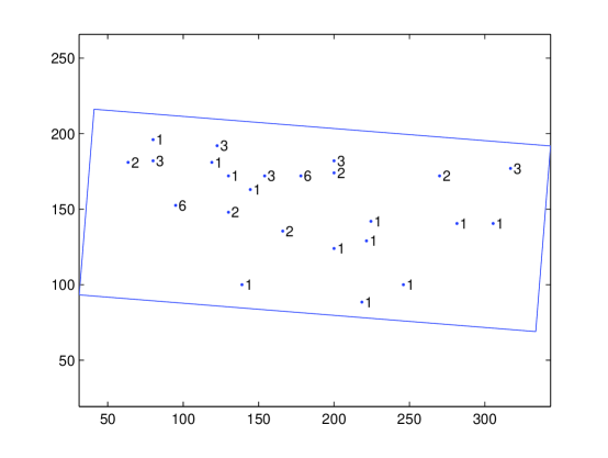
Figure 2: The scatter of pit locations, and the number of dated specimens in each pit which were retained in the analysis. The box marks the edges of the onset-field we will model and has been aligned to the data. The sea is adjacent to the upper edge of the box, with the short box axis pointing towards the sea, and the long axis pointing along the beach. Axes give excavation coordinates.

Criteria for selection for dating included secure association with cultural remains, for example, human burials and diagnostic forms of decorated pottery. The pits were excavated over several years, and dated incrementally, under funding constraints which varied through time. There is a need to date across the site in three spatial dimensions, so material selected for dating is to some extent deliberately spread out.

There is a conjecture, described in Nunn (2007, 2009), that a small initial settlement in the centre of the beach grew in size to eventually cover the studied site area. We formalise this conjecture, and compute the posterior probability that it is true, along with other measures of support. We make a spatio-temporal map of the date at which the deposition of human-related material began at each point on the site. For each spatial location, this “onset-field” map gives the time at which the deposition rate changes from zero to some positive value. The inference is conditioned to ensure that the pit locations and the distribution of dated specimens across pits are not by themselves informative of variations in the time-span of human activity from pit to pit.

We begin our modeling of the data with a description, in Section 4, of a family of prior models for the joint distribution of specimen ages. These temporal models, developed in Naylor and Smith (1988); Zeidler et al. (1998); Nicholls and Jones (2001) and implemented in the OxCal software described in Ramsey (2001), are in widespread use. The dated-specimen deposition process is a Cox process in time. Specimen ages are the times for events in a Poisson point process, which has a rate which may vary from pit to pit, but is constant in time between change points. The site-wide dated-specimen deposition process is the sum of independent Poisson processes in each pit (the specimen are all small pieces of charcoal and shell and would have been waste material at the time). Change points are the boundaries of phases of deposition. In this class of models, the number of change points is known from separate evidence. Phase boundaries mark site-wide changes in the human activities generating dateable specimens and may be indicated by strata. The phase boundaries are modeled as events in a second constant rate Poisson point process. The rate parameters (for specimen ages, and phase boundary ages) are not usually physically interesting, or easy to model, as the ages of dated specimens are the ages of events in an original deposition process thinned by arbitrary specimen selection at excavation, and the uneven action of decay. It is not necessary to estimate these rates if we can condition the analysis on the number of phases, and the number of dates in each phase. This is possible, for example, if phases are strata and a fixed number of specimens are taken temporally at random within known strata.

In our spatio-temporal model, described in Section 5, an onset-time field replaces the earliest phase boundary of the temporal phase model of Section 4. This allows the start-time for the deposition of dateable material to be a function of position. The phase and dated-specimen processes are otherwise unchanged. The onset-field process is a two-parameter spatio-temporal process on a rectangular lattice, and is related to the family of models described in Richardson (1973). One parameter of the onset-field process controls the rate at which an unoccupied cell is occupied by “immigration from off-site” and the other the rate for cell occupation from neighboring occupied cells. For suitable parameter choices, the field can vary from a simple space-time cone, developing like a solution to the non-linear Fisher equation in a wave-of-advance, to a randomly corrugated surface. A prior sample is shown in Fig. 3.

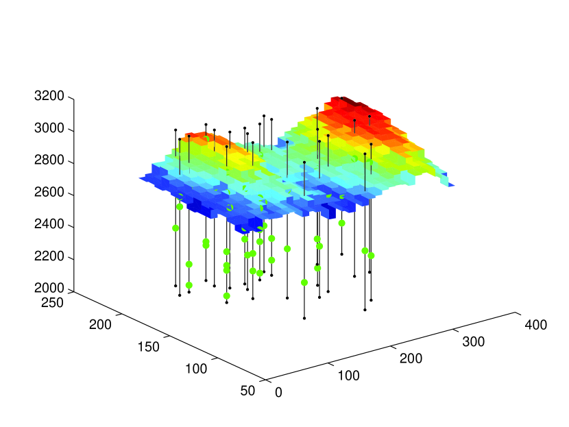
Figure 3: A realization of the prior of Section 5.3 for specimen ages $\theta$ (green dots), phase boundaries (black dots, for a single phase, $M=1$), onset-field $\phi$ (piecewise constant surface of $32\times 13$ cells) for $\alpha$,$\beta_{1}$ and $\beta_{2}$ distributed with $A=10$ and $B=1$ in Equation (8) and limits $L=2000$, $U=3500$ years BP. (z-axis) years BP, (x,y-axes) 0.25cm units.

Further aspects of the model are illustrated in the supplement. We fit this model in Section 6, allowing just one phase, since there is no given phase structure for the Bourewa data. In this model, dated specimens are generated in a single interval with a spatially varying onset-time and a finishing time which is the same everywhere. The dated-specimen deposition process has a rate which is assumed constant in time when it is non-zero, but may have arbitrary spatial structure. Because we condition the analysis on the number of dates in each pit and on the number in each phase (there is only one phase), there are no deposition rate parameters left to estimate.

In the remainder of the paper we fit extensions to the single-phase onset field model. However, the model in Section 6 has a good balance of realism and simplicity, and the further development may be read as model mis-specification testing. Is there really just a single phase, and if not, what temporal variation is present? Although there is no evidence from stratigraphy for phase structure for the Bourewa data, it is possible that some phase structure is present. This possibility is implicit in the analyses of Nunn (2007, 2009) and is a second question (besides the settlement hypothesis) of archaeological interest.

The third model, which we describe in Section 7, is a non-parametric extension of the basic phase model of Section 4, with no spatial structure. The number of change points in the deposition rate between the beginning and end of deposition is unknown. Since the phase structure is unknown, we can no longer condition on the assignment of specimens to phases. We need therefore to model the ratio of deposition rates between phases, in order to weight the assignment of dates to phases. Significant variation in the accumulation rate of specimen dates is evidence for phase structure. However, although evidence for two or more phases is evidence for rate variation, the phases we reconstruct need not be culturally significant. We fit the phase structure model of Section 7 to the Bourewa data in Section 7.2.1 and get results which are misleading in just this way. We therefore test this third model in Section 7.2.2 with an application to a second data set, the Stud Creek radiocarbon data, published by Holdaway et al. (2002). For these data there is a hypothesis that the original deposition was interrupted for some time. We reject the single-phase model in favor of a three phase model. We are at this point fitting a change-point process of unknown piece-wise constant rate, with no spatial component. Green (1995) uses a temporal change-point analysis of coal-mining fatalities data to illustrate reversible-jump MCMC. Our event times are observed with the radiocarbon uncertainty, but the analysis is, at this point, otherwise the same.

We return in Section 8 to the Bourewa data to fit a model with the randomly variable temporal phase-structure of Section 7 and the spatio-temporal onset-field of Section 5. In this fourth and final model, we start deposition with a spatially varying onset field and follow this with an unknown number of phases. We condition on the assignment of dates to pits, but not the assignment of dates to phases. The assignment of a specimen to a phase depends on the ratios of deposition rates between phases, as in Section 7. We assume that these ratios do not vary from pit to pit. This reduces the number of unknown rate parameters to a small number, one less than the (unknown) number of phases. The assumption is good if, for example, it was true for the original deposition, and the uneven thinning due to specimen selection and decay is separable, so that the thinning probability is the product of one function of space and another of time.

2 Related literature

Discusion of related literature on the Richardson process itself is given in Section 5.2.

2.1 Methodology

Majumdar et al. (2005) give a Bayesian statistical framework for the analysis of spatio-temporal data with a single change point. They note that the framework is easily generalised, and illustrate it by fitting a Gaussian process $Y(s,t)$ $s\in\Re^{2}$, $t\in\Re$ with a change point at time $t=t_{0}$. The process changes from $\mu_{t}+U(x,t)+W(x,t)+\varepsilon(x,t)$ at $t\leq t_{0}$ to $\mu_{t}+U(x,t)+W(x,t)+\varepsilon(x,t)$ at $t>t_{0}$. Here $\varepsilon(x,t)$ is a field of independent normal random variables, and $U$, $V$ and $W$ are Gaussian processes with separable translation-invariant covariance functions. These data are observed at $N$ points in space at each of $M$ points in time. In their successful simulation study they fit fourteen parameters to data: the scalar means and variances of $\varepsilon$ either side of $t_{0}$ (four), the space and time scales of the exponential class correlation functions for $U,V$ and $W$ (six) and their three variance-scaling parameters, plus $t_{0}$ itself. Our own fitting assumes complete spatial independence between specimen-deposition events at different pits, conditional on the unknown deposition rate. On the other hand, we do not know the deposition rates, or the number of change points, and the onset field is a new kind of change-point, since it is a change-field which spreads gradually over the region, marking the transition from zero to non-zero deposition rate. Ibáñez and Simó (2007), who wish to model change-points which spread in this way, have suggested a modification of Majumdar et al. (2005), though there is to date no fitting.

We found few applications of Bayesian or likelihood-based inference for spatial-temporal growth processes. Zhu et al. (2008) fits a complex, and relatively realistic model to beetle presence and count data and tree-mortality data for two beetle species and the tree-health indicator simultaneously. The two species compete and spread on a random graph with trees at nodes. Time is discrete corresponding to year. The likelihood for the process is given as a Markov Random Field up to an unknown normalising constant. The process (beetle counts, tree state) is observed directly. Our onset-field is similar: the process is spread $via$ neighbors, and immigration. The probability density for the onset-field process here is given as an MRF also, though our simpler process is normalisable. However, our onset-process is observed indirectly, through the events which follow it, and it is this aspect, its role as a change point, which distinguishes the applications.

Møller and et al. (2008) fit data for a point process $\mathbf{X}_{t}$ of bush-fire locations and discrete times allowing a spatially structured intensity of the form $\lambda(x,t)=\lambda_{1}(x)\lambda_{2}(t)S(x,t)$ with ${\sf E}(S(x,t))=1$ and $(x,t)\in\Re^{2}\times\mathbb{Z}$. The components $\lambda_{1}$ and $\lambda_{2}$ are given in terms of linear predictors from covariates for spatial and temporal structure respectively and Møller and et al. (2008) take a shot-noise process for the residual process $S(x,t)$. Diggle et al. (2005) set this framework up to model spatial-temporal disease data, with a unit mean log-Gaussian residual process. Because the likelihood is intractable, Møller and et al. (2008) develop alternative estimation procedures, including Lindsay’s composite likelihood. The aim in Diggle et al. (2005) and Møller and et al. (2008) is to model the bulk point process in 2+1D. In contrast, our data collapse the spatial locations of dated specimens in a pit (which has some extension) onto a single point, and events in each pit are modeled using a process which is marginally a 1D Cox process. Separable intensities play a role in all the spatial-temporal statistical analyses we have cited, including our own.

2.2 Application

Where there is an interest in recovering unknown phase structure without spatial structure, many authors sum the likelihood functions for individual specimen ages to get a single function of age. Holdaway et al. (2008) is a rare example in which this procedure may be justified. Under certain conditions, the summed likelihood is an estimate of the dated-specimen deposition-rate function. Bayliss et al. (2007) warn against the common practice of treating this as a proxy for population density.

Spatial maps based on the distribution of radiocarbon ages are not usually model based, but simply a sequence of scatter plots of find locations windowed by age, as Graham et al. (1996). One dimensional projections of 2D data, such as the compilation of early European-Neolithic dates by Ammerman and Cavalli-Sforza (1971), who projected on distance-from-Jericho, are commonly regressed. Hazelwood and Steele (2004) give a recent overview of the same subject, and make a comparison with the settlement of North America, in two spatial and one temporal dimension. These authors fit a Fisher wave-of-advance model using a linear regression to get the wave speed, and guess plausible values for other model parameters based on prior knowledge of generic human demography. In the latest work in this spirit, Davison et al. (2009) map the Neolithic settlement of Europe, modeling non-interacting expansion from two sources, using a Fisher wave-of-advance model with parameters for growth rate, carrying capacity, spatially varying 2D advection and a scalar diffusivity. They pool or otherwise reduce the earliest dates at a given location to form a central estimate for the local arrival of the Neolithic peoples. They fix model parameters using a hybrid scheme. Initial conditions, such as the starting locations and times of the two expansions, are obtained by minimizing the root mean square difference between the reduced date at each location and the arrival time of the modeled population wavefront at that location. This is nonlinear regression. Parameters of the advection-diffusion are fixed using prior knowledge of generic human demography, as in Hazelwood and Steele (2004). Note that, although these authors do not make likelihood-based inference, they are modeling an onset-field.

Blackwell and Buck (2003) treat a collection of radiocarbon dates from a number of sites excavated under different conditions at different times over northern Europe. For such spatially sparse data it is not useful to couple the onset event at each site with a smooth spatial field. They group the data into regions, and fit an independent temporal model for each region. Since the analyses are not spatially coupled, Blackwell and Buck (2003) page 238 describe their own analysis as “not truly spatiotemporal in nature”. In contrast, the data we treat comes from a single intensively studied site. Dated pits are dense in the modeled region. These properties of the Bourewa data justify some spatial smoothing of the field of onset times.

3 Data, and observation model

The data are $K=60$ uncalibrated radiocarbon ages $y_{i},i=1,2,\dots K$, with associated laboratory standard errors $\sigma_{i}$, grouped in $H=32$ pits. Some of these data were dropped as discussed in the final paragraph below. For pit number $h=1,2,\dots,H$, $x_{h}=(x_{1,h},x_{2,h})$ gives pit coordinates. Let ${\bf h}(i)$ map data index to pit index. The location $x_{{\bf h}(i)}=(x_{1,{\bf h}(i)},x_{2,{\bf h}(i)})$ of the $i^{\prime}th$ dated specimen is given as a point-location for the pit in which it was found, although pits vary in size from 0.25 to 2 meters on each side. Some pits are dug but not dated. Dated pits are distributed over a region approximately 200 by 50 meters, with the majority of pits in a cluster some 50 meters square.

Denote by $\Theta_{i}$ the unknown true age of the $i$’th dated specimen, measured in calendar years before 1950 (Before the Present, BP). Observations of specimen ages are distorted by a non-linear, empirically determined, calibration function $\mu$, with associated error function $\sigma$. In the standard observation model of Stuiver and Polach (1977); Buck et al. (1992),

$$Y_{i}=\mu(\Theta_{i})+\epsilon_{i}$$

with $\epsilon_{i}\sim N(0,\sigma_{i}^{2}+\sigma(\Theta_{i})^{2})$ independent random variables. We are omitting some straightforward details: marine and terrestrial material are in fact calibrated using different calibration functions and radiocarbon ages measured on local seashell are subject to the small constant marine-reservoir offset given in Nunn (2007), which we treat as discussed in Jones and Nicholls (2001). In our software we use the 2004 calibration functions of McCormac et al. (2004) and Hughen et al. (2004) interpolated from their calibrations at 5 year intervals down to one year intervals, and then approximate $\Theta_{i}$ as an integer year. In our discussion here $Y$ and $\Theta$ are continuous.

The normal likelihood for parameters $\Theta=\theta$ given data $Y=y$ is

$$\ell(\theta;y)\propto\prod_{i=1}^{K}(\sigma_{i}^{2}+\sigma(\theta_{i})^{2})^{-1/2}\exp\left(-\frac{(\mu(\theta_{i})-y_{i})^{2}}{2(\sigma_{i}^{2}+\sigma(\theta_{i})^{2})}\right)$$

with $\mu$ and $\sigma$ functions of $\theta$ available from a look-up table. The likelihoods of the Bourewa specimen ages are graphed in Fig. 1. Certain specimens (blue points) were dropped from the analysis as either insecurely linked to evidence of human presence, or associated with activity outside the period of interest. Some pits containing a single omitted specimen were thereby removed from the analysis. Data from two pits lying far from the central area were dropped as the spatial extrapolation to those isolated pits was deemed too great, leaving the $H=24$ pits and $K=49$ radiocarbon dates represented in Fig. 2.

4 Conditioning on phase structure

The posterior distribution specified in this section can be simulated using existing OxCal software. However, the notation of this section is needed below, and the numerical results will be of interest because, although obtained from standard models in the literature, they conflict with the results we get from the onset-field model.

We begin with a prior model of the process generating dates in a single pit. Dates within a pit are grouped into phases, corresponding to some form of strata. The ages $\Theta_{i},\Theta_{j}$ of specimen from distinct strata are known a priori to be ordered, so that $\Theta_{j}>\Theta_{i}$ if specimen $j$ is from a deeper stratum than that of specimen $i$. Denote by $\Psi_{m},m=0,\dots,M$ the unknown true age of the $m$’th phase boundary, with $\Psi_{m}<\Psi_{m+1}$, so that numbering is from the surface to the bottom of the pit, and the $m$’th phase is the age interval $[\Psi_{m-1},\Psi_{m}]$. Let ${\bf m}(i)$ give the known phase ($ie$, stratum) of the $i$’th dated specimen. Phases may be empty, with no specimen taken from the corresponding stratum, as happens if for example there is a hiatus in deposition, or possible erosion. Let $L$ and $U$ be fixed lower and upper bounds on specimen and phase boundary ages, available as prior knowledge. We use $L=2000$ and $U=3500$ years BP except in Section 7.2.2. The parameter state space for analysis of a single pit is

$$\Omega=\{(\psi,\theta):L<\psi_{0},\ \psi_{m-1}<\psi_{m}\ m=1,..,M,\ \psi_{M}<U,\ \psi_{{\bf m}(i)-1}<\theta_{i}<\psi_{{\bf m}(i)}\ i=1,..,K\}.$$

We follow Nicholls and Jones (2001), who get a prior density for $(\Psi,\Theta)$ by modeling the deposition process generating those parameters. The phase boundaries $\Psi_{1},\dots,\Psi_{M-1}$ are the events of a Poisson point process $\Lambda_{\Psi}$ of constant rate $\lambda_{\psi}$ which starts at the onset-time $\Psi_{M}$ and stops at the ending-time $\Psi_{0}$. Nicholls and Jones (2001) prior density for onset and ending times $\Psi_{M}=\psi_{M}$ and $\Psi_{0}=\psi_{0}$ is $p_{0,M}(\psi_{0},\psi_{M})=(U-L-(\psi_{M}-\psi_{0}))^{-1}$ and this leads to a joint prior density $p(\psi|M)$ at $\Psi=\psi$ equal to

$$p(\psi|M)=\frac{1}{(U-L-(\psi_{M}-\psi_{0}))}\frac{1}{(\psi_{M}-\psi_{0})^{M-1}}.$$ (1)

This density has a uniform marginal distribution for the span statistic, $\Psi_{M}-\Psi_{0}\sim U(0,U-L)$. This is desirable when the span is of particular interest, as is often the case (though Naylor and Smith (1988) make $p(\psi|M)=1$ favoring greater spans over lesser). The specimen ages $\Theta_{1},\dots,\Theta_{K}$ are the events of a Poisson point process of piece-wise constant rate $\lambda_{\theta}(t)=\lambda_{\theta,m}$ for $\psi_{m-1}<t<\psi_{m}$. The rates $\lambda_{\theta,m}$ are not of interest, since the archaeologist imposes an uneven thinning on specimen, in selecting specimen for dating, on top of possible uneven thinning by in situ decay. However, since the analysis is conducted conditional on the number $M$ of phases, and conditional on specimen phases ${\bf m}$, the conditional density for $\Theta|\Psi$ is

$$p(\theta|\psi,{\bf m})=\prod_{i=1}^{K}(\psi_{{\bf m}(i)-1}-\psi_{{\bf m}(i)})^{-1}.$$ (2)

The posterior distribution is

$$p(\psi,\theta|y,{\bf m},M)=\ell(\theta;y)p(\psi,\theta|M,{\bf m}),$$ (3)

with

$$p(\psi,\theta|M,{\bf m})=p(\theta|\psi,{\bf m})p(\psi|M)$$

given by Equations (1) and (2).

In this kind of analysis, a site is treated as in effect a single pit. Fitting this model to the Bourewa data, for a single phase, $M=1$, so ${\bf m}(i)=1$ for each $i=1,2,\dots,K$ using the MCMC algorithm given in Nicholls and Jones (2001) to sample the posterior distribution of Equation (3), we get the marginal posterior distributions for onset age $\psi_{M}$ and ending age $\psi_{0}$ shown in green in the leftmost column of Fig. 4.

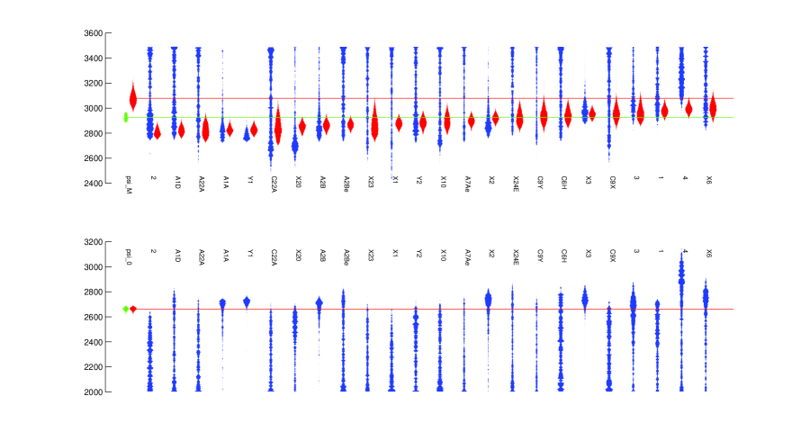
Figure 4: (top) posterior distributions of onset-times ($\psi_{M}$ or $\phi_{{\bf c}(h)}$, y-axis, years BP) by pit (pit-names, x-axis, sorted by median onset). (bottom) posterior distributions of ending times $\psi_{0}$. Leftmost histograms labeled $\tt psi\_M$ are (red) $\psi_{M}$ for the onset field analysis of Section 6 and (green) $\psi_{M},\psi_{0}$ for all dates in single phase, as Section 4. The remaining columns are (red) onset-field interpolations $\phi_{{\bf c}(h)}$ and (blue) $\psi_{M},\psi_{0}$ from an independent single phase analysis (as Section 4) of the data from the pit for that column.

As part of a later model mispecification analysis, we fit the (single phase) model of this section to each pit independently, including pits with just one or two dated specimens (for which the posterior distribution of $\psi_{1}$ and $\psi_{0}$ is dominated by the choice of the upper and lower limits, $U$ and $L$). These distributions are displayed in blue and labeled by pit name in Fig. 4.

5 A spatial-temporal onset-field model

The whole process is started at the first-onset time $\psi_{M}$. This is “first settlement”. The onset field begins to evolve, as the area in use is enlarged by spreading out, and by new arrivals. New phase events at times $\psi_{M-1},\dots\psi_{1}$ are step-changes in the deposition rate across the then-occupied site, corresponding to changes in the way the then-occupied site is used. The deposition process terminates at the ending event, at time $\psi_{0}$.

5.1 The onset-field process

Let $\phi_{c},\ c=1,2,\dots,C$ be a field $\phi_{c}\leq\psi_{M}$, defined on a rectangular $C_{1}\times C_{2}$ lattice of $C=C_{1}C_{2}$ square cells. Let ${\mathcal{N}}(c)$ give the set of neighbors of the $c$’th cell. Corner, side and interior cells have two, three and four nearest neighbors respectively. Let ${\mathcal{N}}^{+}(c)={\mathcal{N}}(c)\cup\{c\}$. Let ${\bf c}(x)$ map points $x$ in the pit coordinate system to the index of the overlaying lattice cell. A modeled pit has a point-like location, though it may lie cross cells. We report results for a $13\times 32$ lattice of cells each about 2.375 meters square.

The variable $\phi_{c}$ gives the onset time for deposition at points $x$ in cell $c={\bf c}(x)$. The onset time $\phi_{c}$ in cell $c$ is the time of first occupation for cell $c$. There is one arrival in each cell and $C$ arrivals in the course of the process. Let $r_{c,n}$ give the arrival rate in cell $c$ in the time interval preceeding the $n$’th arrival in the process, and let $R_{n}=\sum_{c}r_{c,n}$ give the total arrival rate in the $n$’th interval. Let $L<\psi_{0}<\psi_{1}<\dots\psi_{M}<U$ and for $c=1,2,\dots,C$ and $c^{\prime}\in{\mathcal{N}}(c)$ let positive constants $\alpha_{c}$ (the rate for immigration to cell $c$) and $\beta_{c,c^{\prime}}$ (the rate for occupation of cell $c^{\prime}$ from occupied cell $c$, with $\beta_{c,c^{\prime}}=\beta_{c^{\prime},c}$) be given. We call the process parameterised by $\beta$ ‘migration’.

The onset-field $\phi$ is a realization of the following immigration-migration process: cell $c$ is occupied by immigration at rate $\alpha_{c}$; when cell $c$ becomes occupied, the arrival rate for occupation at each of its neighbors $c^{\prime}\in{\mathcal{N}}(c)$ is increased by $\beta_{c,c^{\prime}}$. A cell once occupied stays occupied. When we fit data, we will condition on the first onset-field event occurring at $\psi_{M}$ years BP; the algorithm below is for the unconditional case.

Step 1

Initialize field of rates

Step 1.1

$t_{0}\leftarrow\psi_{M}$, $r_{c,1}\leftarrow\alpha_{c}$ for each $c=1,2,\dots,C$ and $R_{1}=\sum_{c}r_{c,1}$.

Step 1.2

Set $n\leftarrow 1$.

Step 2

Simulate arrivals at Exp$(R_{n})$ intervals:
while $R_{n}>0$

Step 2.1

simulate $\delta_{n}\sim\mbox{Exp}(R_{n})$ and $c_{n}\sim(r_{1,n}/R_{n},r_{2,n}/R_{n},\dots,r_{C,n}/R_{n})$;

Step 2.2

Set $t_{n}\leftarrow t_{n-1}-\delta_{n}$ and $\phi_{c_{n}}\leftarrow t_{n}$. For each $c=1,2,\dots,C$, set $r_{c,n+1}\leftarrow r_{c,n}$ and then overwrite $r_{c_{n},n+1}=0$ and $r_{c,n+1}\leftarrow r_{c,n+1}+\beta_{c_{n},c}$ for each $c\in{\mathcal{N}}(c_{n})\setminus\{c_{1},c_{2},\dots,c_{n-1}\}$.

Step 2.3

set $n\leftarrow n+1$.

We orient the lattice along the beach, and allow the rates for migration along and at right angles to the long axis of the beach to be unequal. We fit fields for $\alpha_{c}=\alpha$ and $\beta_{c,c^{\prime}}=\beta_{1}$ for $c\rightarrow c^{\prime}$ along the beach and $\beta_{c,c^{\prime}}=\beta_{2}$ for $c^{\prime}$ closer to, or further from, the sea. If $\alpha$ is small, and $\beta_{1}=\beta_{2}=\beta$ is large, typical onset fields show a spread from a single centre. A 2+1D plot is cone-like. As $\alpha$ increases at fixed $\beta$, the number of centres-of-expansion increases, corresponding to isolated settlements which grow and merge.

The onset-field model is convenient for fitting. The joint density $p(\phi|\alpha,\beta,\psi)$ of $\phi$ is

$$p(\phi|\alpha,\beta,\psi)=\prod_{n=1}^{C}r_{c_{n},n}\exp(-R_{n}\delta_{n}),$$

from the algorithm. Now

$$\sum_{n}R_{n}\delta_{n}=\sum_{c=1}^{C}\left[\alpha_{c}(\psi_{M}-\phi_{c})+\frac{1}{2}\sum_{c^{\prime}\in{\mathcal{N}}(c)}\beta_{c,c^{\prime}}|\phi_{c}-\phi_{c^{\prime}}|\right].$$

Each cell $c$ contributes to $\sum_{n}R_{n}\delta_{n}$ a term $\alpha_{c}(\phi_{c}-\psi_{M})$ and for each neighbor $c^{\prime}$, a term $\beta_{c^{\prime},c}(\phi_{c^{\prime}}-\phi_{c})\mathbb{I}_{\phi_{c}<\phi_{c^{\prime}}}$. Taking the two such terms for each edge gives $\beta_{c,c^{\prime}}|\phi_{c}-\phi_{c^{\prime}}|$. Let $\rho(\phi_{{\mathcal{N}}^{+}(c)})$ be the rate function of $\phi_{c}$,

$$\rho(\phi_{{\mathcal{N}}^{+}(c)},c)=\alpha_{c}+\sum_{c^{\prime}\in{\mathcal{N}}(c)}\beta_{c,c^{\prime}}\mathbb{I}_{\phi_{c^{\prime}}>\phi_{c}},$$ (4)

so that $\rho(\phi_{{\mathcal{N}}^{+}(c_{n})},c_{n})=r_{c_{n},n}$. This is the arrival rate for occupation of cell $c$ in the time interval preceding $\phi_{c}$, and $\phi_{c}$ is an age BP, so that interval is ages greater than $\phi_{c}$. Assembling these terms gives

$$p(\phi|\alpha,\beta,\psi)=\prod_{c=1}^{C}\exp\left(\log(\rho(\phi_{{\mathcal{N}}^{+}(c)}),c)-\alpha_{c}(\psi_{M}-\phi_{c})-\frac{1}{2}\sum_{c^{\prime}\in{\mathcal{N}}(c)}\beta_{c,c^{\prime}}|\phi_{c}-\phi_{c^{\prime}}|\right).$$ (5)

The right hand side is normalized over $\phi\in(-\infty,\psi_{M}]^{C}$ so inference for $\alpha$ and $\beta$ is not obstructed by an intractable normalization. Also, $\Phi$ is a Markov Random Field (MRF) with cliques $\{c\},\{c,c^{\prime}\}_{c^{\prime}\in{\mathcal{N}}(c)}$ and ${\mathcal{N}}^{+}(c)$.

5.2 The Richardson growth model, and related models

The onset-field process is a special case of the contact process with immigration. Cells of a contact process, occupied by the immigration and migration processes above, are abandoned at per capita rate $\gamma$; a binary field $\xi_{c}(\tau),\ c=1,2,\dots,C,\ \tau\in[0,\infty)$ indicates if a cell is occupied at time $\tau$. The process is often studied without immigration, conditioned on one or more arrivals, or seeds, at time $\tau=0$. The equilibrium statistics of $\xi$ are studied, as functions of $\beta$ and $\gamma$. Durrett and Levin (1994) review the process in the context of applications in ecology. A contact process in which a single cluster of occupied cells grows from a single seed, with no immigration or abandonment ($\alpha=\gamma=0$), is a Richardson cluster-growth model, so the onset-field model above is a Richardson model with multiple clusters, $ie$, with immigration. Richardson (1973) showed that the cluster grows linearly and tends in shape towards some fixed shape. Durrett and Liggett (1981) extend this, giving further results for the boundary shape. If the process is isotropic, this limiting shape is a circle. Hammersley (1977) and Durrett and Liggett (1981) are sceptical. However, the limiting shape is not known at present. The simulation experiments reported in the Supplement show that it is at least very nearly isotropic. This is important as we would like the process at $\beta_{1}=\beta_{2}=\beta$ to be isotropic, for clarity of interpretation.

Lee (1999) uses a Richardson process with a Poisson number of randomly located seeds to model fields of aluminium grains as random lattice segmentations. The cluster seeds all ’arrive’ at the start time. The process realizes a random segmentation of the lattice into regions labeled by the index of their seed. Lee (1999) conjectures that, for his initialisation, the large scale structure of the $\alpha=0$, $\gamma=0$ process is isotropic, and for fixed seeds the region borders converge to the edges of a Voronoi tesselation as the cells are subdivided.

Because our seeds arrive at different times, the onset-field process generates a segmentation which looks something like a Johnson-Mehl tesselation at large scale. Johnson-Mehl tesselations, described for example in Møller (1999), are random tesselations of the plane continuum. Seeds arrive in $\mathbb{R}^{2}\times[0,\infty)$ according to a Possion process in two space and one time dimension. Each seed captures a circular domain which grows with a fixed speed until it meets the boundary of another domain. Seeds falling into existing domains are deleted. This continuum version of the process we are using, with deterministic region growth, would be a natural off-lattice model, which we have not considered.

See the supplement for further discussion of the stationarity and isotropy of the onset-field process, and a relation to traveling wave models.

5.3 The onset-field as a prior probability density for the Bourewa data

The full prior density for the inference in the next section is

$$p(\alpha,\beta,\theta,\phi,\psi|M,{\bf m})=p(\theta|\phi,\psi,{\bf m})p(\phi|\alpha,\psi,\beta,\max(\phi)=\psi_{M})p(\psi|M)p(\alpha,\beta).$$ (6)

Prior density $p(\psi|M)$ is given Equation (1). We condition the onset-field on $\max(\phi)=\psi_{M}$; in terms of model elements, this means that the beginning of the earliest phase coincides with first settlement, and spreading occupation. The modification is

$$p(\phi|\alpha,\beta,\psi,\max(\phi)=\psi_{M})=\alpha^{-1}p(\phi|\alpha,\beta,\psi)$$

for $p(\phi|\alpha,\beta,\psi)$ given in Equation (5), and

$$\phi\in\{\phi:\phi\in(-\infty,\psi_{M}]^{C},\max(\phi)=\psi_{M}\}.$$

Although we now drop $\max(\phi)=\psi_{M}$ in our notation, all the distributions below which involve $\phi$ are conditioned in this way. The onset field fixes the local change point from zero to non-zero rate for dated-specimen deposition. This imposes

$$\psi_{{\bf m}(i)-1}<\theta_{i}<\min(\phi_{{\bf c}(x_{{\bf h}(i)})},\psi_{{\bf m}(i)}).$$

The bound on the right hand side is the change-point to a non-zero deposition rate, so we should replace the density for $\Theta|(\Psi,{\bf m})$ given in Equation (2) with

$$p(\theta|\phi,\psi,{\bf m})=\prod_{i=1}^{K}\frac{1}{\min(\phi_{{\bf c}(x_{{\bf h}(i)})},\psi_{{\bf m}(i)})-\psi_{{\bf m}(i)-1}}.$$ (7)

The onset field can be thought of as a spatio-temporal mask over temporal phase structure which would otherwise apply at all locations.

Our prior for $\alpha$ and $\beta$ is subjective. We expect just a handful of pure immigration events in the interval $[L,U]$, so we need ${\sf E}(\alpha)\gtrsim 1/C(U-L)$. The “speed” of the expansion is controlled by $\beta$ and for small $\alpha$ is between $2\beta$ and $3\beta$ [cells/year] (see supplement for further discussion on this point). If the expansion is to cover the site in the interval $[L,U]$ then we need

$${\sf E}(\beta)\gtrsim\frac{\max(C_{1},C_{2})}{2(L-U)}.$$

Rate parameters $\alpha$ and $\beta$ are otherwise positive so the maximum entropy priors are

$$\alpha\sim\mbox{Exp}(A/N(U-L)),\quad\beta\sim\mbox{Exp}(B\max(C_{1},C_{2})/2(L-U)).$$ (8)

Prior simulation showed $1\lesssim A\lesssim 20$ and $0.5\lesssim B\lesssim 2$ generated a range of onset-fields with plausibly varied temporal “roughness” (increasing with $\alpha$) and “peak to valley depth” (decreasing with $\beta$).

The onset-field process has a boundary effect. In realizations of the process, boundary cells are typically occupied later than cells in the interior. Since

$$\int_{(-\infty,\psi_{M}]^{C}}p(\phi|\alpha,\beta,\psi)d\phi=1,$$

we can differentiate with respect to $\alpha_{c}$ to get the moment identity

$${\sf E}(\phi_{c})=\psi_{M}-{\sf E}\left(\frac{1}{\alpha_{c}+\sum_{c^{\prime}\in{\mathcal{N}}(c)}\beta_{c,c^{\prime}}\mathbb{I}_{\phi_{c^{\prime}}>\phi_{c}}}\right).$$ (9)

Since corner and side cells have fewer neighbors than interior cells, the sum $\rho(\phi_{{\mathcal{N}}^{+}(c)})$ in the denominator Equation (9) is distributed over a smaller total there. Differentiating again with respect to $\alpha_{c^{\prime}}$ gives

$${\sf E}\left(\left(\phi_{c}+\frac{1}{\rho(\phi_{{\mathcal{N}}^{+}(c)})}-{\sf E}\left(\phi_{c}+\frac{1}{\rho(\phi_{{\mathcal{N}}^{+}(c)})}\right)\right)\left(\phi_{c^{\prime}}+\frac{1}{\rho(\phi_{{\mathcal{N}}^{+}(c^{\prime})})}-{\sf E}\left(\phi_{c^{\prime}}+\frac{1}{\rho(\phi_{{\mathcal{N}}^{+}(c^{\prime})})}\right)\right)\right)=0,$$

so $\phi_{c}+\rho(\phi_{{\mathcal{N}}^{+}(c)})^{-1}$ and $\phi_{c^{\prime}}+\rho(\phi_{{\mathcal{N}}^{+}(c^{\prime})})^{-1}$ are uncorrelated, and we have verified this numerically, as a check on our code. The field of values $\phi_{c}+\rho(\phi_{{\mathcal{N}}^{+}(c)})^{-1}$ is homogeneous and isotropic to 2nd order, regardless of boundary effects. Further field identities are given in Section 5.1 of the Supplementary material.

We might pad the site with a large border outside the area where pits are concentrated, or, considering Equation (9), raise $\alpha_{c}$ for $c$ the index of a boundary cell. However, simulation of $p(\alpha,\beta,\phi|\psi)$ showed that these approaches give a distribution of onset fields which does not represent prior belief for this site. If there are just a few immigration events, and the field is extended a great deal, then the immigration events tend to occur in the extension, and the pit-area is settled by migration. In this class of models, the interval between the onset event at time $\psi_{M}$ (people arrive on the beach) and occupation at cells covering pits (the settlement reaches the excavated area) can be improbably large. By accepting some spatial inhomogeneity in the prior onset-field at the boundary we get a prior distribution better resembling prior belief.

Pit locations are a second source of spatial inhomogeneity. The location of a pit with at least one dated specimen is informative for the onset field, without the radiocarbon date itself, because the deposition process must act for some finite time wherever there are dated specimens. This constrains $\phi_{{\bf c}(x_{h})}>\psi_{0}$ for $h=1,2,\dots,H$, but not elsewhere. We go further and assert as part of the observational data that the deposition process acts for some finite time at each point over the windowed region of this site, so $\psi_{0}<\phi_{c}\leq\psi_{M}$. Conditional on this assertion, the locations of the dated pits are not informative. As a side-effect, the marginal prior distribution of the span $\psi_{M}-\psi_{0}$ depends on the priors for $\alpha$ and $\beta$. Short spans are excluded at small $\beta$ as the field needs time to cover the site. As a second side effect, the boundary effect mentioned in the previous paragraph is slightly reduced.

A single sample from the prior $p(\theta,\psi,\phi,\alpha,\beta)$ given above, for $M=1$ is shown in Fig. 3. The lattice is $32\times 13$ and $A=10$ and $B=1$. Cells are 2.375 meters on each side, and the field is piecewise constant by cell. In Fig. 5

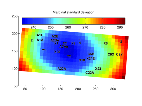
Figure 5: The prior mean onset field (left) and the prior standard deviation of the field (right), in the single-phase onset-field model of Section 5.3. The colors in the color bar give years BP.

we show the prior mean and standard deviation of the field estimated marginally for each cell. Further figures illustrating the onset-field prior and the priors for $\psi$ and $\theta$ are shown in the Supplement. We see residual inhomogeneity in the prior of about 150 years from centre to corner. The marginal prior standard deviation of $\phi_{c}$ at cell $c$ is of order 250 years. This includes random offset variation from $\psi_{M}$, the initialisation-time. The standard deviation of the elapsed time $\psi_{M}-\phi_{c}$ is of the order of 200 years.

6 Fitting the onset-field for a single phase

The posterior density for deposition in a single phase ($M=1$), modeled as Section 4, with the onset-field of Section 5 conditioned to satisfy $\phi\in[\psi_{0},\psi_{M}]^{C}$ is

$$p(\alpha,\beta,\phi,\psi,\theta|y,{\bf m},M)\propto\ell(\theta;y)p(\alpha,\beta,\phi,\psi,\theta|{\bf m},M).$$

For $p(\alpha,\beta,\phi,\psi,\theta|{\bf m},M)$ see the definitions at Equation (6).

We fit this model by Metropolis-Hastings MCMC simulation. The updates are those of Nicholls and Jones (2001). New parameters $\alpha$ and $\beta$ are updated via a scaling proposal $z\sim U(1/2,2)$, $\alpha^{\prime}=z\alpha$, $\beta^{\prime}=z\beta$ and jointly with the onset-field in an update with proposal distribution $p(\phi|\psi)p(\alpha,\beta)$. The algorithm is effective when the latter, which updates $\alpha$, the two components of $\beta$ and the field $\phi$, has a reasonable success rate. We have a second onset-field update with proposal distribution $p(\phi|\alpha,\beta,\psi)$, which conditions on the immigration migration rate parameters. The two $\phi$-updates generate new onset-field values at every cell, and are simulated using the algorithm of Section 5.1. The $\phi$ field has a large spatial correlation, with structure on the same scale as the site itself, so single-cell MRF updates proved to be very inefficient. The condition $\phi\in[\psi_{0},\psi_{M}]^{C}$ is implemented by rejecting proposals at the acceptance stage of the MCMC update which do not satisfy the condition, rather than by making proposals from the conditional distribution.

An image of the posterior mean onset-field is shown in Fig. 6.

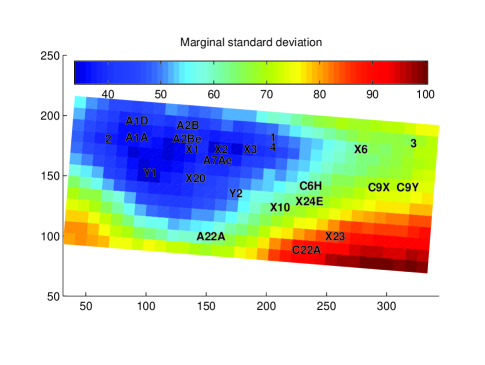
Figure 6: The posterior mean onset field (left) and the posterior standard deviation of the field (right), in the single-phase onset-field model of Section 6.

There is a single peak. Compared to the prior field, Fig. 5, the range of onset times (the depth of the field) has gone up, and the standard deviation, shown in the same figure, has dropped. Typical values (across cells) of the standard deviation of the elapsed times $\psi_{M}-\phi_{c}$ drop from values of order 160 years in the prior to values of order 60 years in the posterior. Fig. 4 shows the posterior distribution for first settlement, $\max(\phi)=\psi_{M}$ (with $M=1$, leftmost red histogram) at around 3100 BP. By contrast the single phase analysis puts this event at around 2900 BP, since it is pulled down by pits with younger dates. Fig. 7

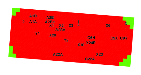
Figure 7: Support for spread: (left) the posterior probability that $\psi_{M}-\phi_{c}<150$ (respectively, $\psi_{M}-\phi_{c}>150$) is greater than 0.8 for cells $c$ in the green (blue) region, in the single-phase onset-field model of Section 6. (right) the corresponding image for the prior distribution of the onset field. Results for the multi-phase onset-field model of Section 8 are similar.

shows the sets of cells

green $$= \{c:\Pr(\psi_{M}-\phi_{c}>T^{*}|y)>p^{*},c=1,2,\dots,C\},$$

blue $$= \{c:\Pr(\psi_{M}-\phi_{c}<T^{*}|y)>p^{*},c=1,2,\dots,C\},$$ (10)

red $$= \{1,2,\dots,C\}\setminus(\mbox{green}\cup\mbox{blue}),$$

with $T^{*}=150$[years] and $p^{*}=0.8$ and we estimate the probabilities using MCMC simulation of $p(\alpha,\beta,\phi,\psi,\theta|y,{\bf m},M)$. Green cells are all settled within 150 years of first arrival, and blue cells are all settled more than 150 years after first arrival, with marginal cell probabilities all at least 0.8. A visually interesting threshold $T^{*}$ was set by searching, so there is a hazard akin to multiple testing. However, when we repeat this exercise on prior simulations no single threshold $T^{*}$ makes both ’green’ and ’blue’ non-empty at $p^{*}=0.8$.

Independent pit-by-pit estimation of the onset and terminal events for a phase model of the kind described in Section 4 ($ie$, without onset field) is usually pointless if there are no more than two dated specimen in each pit. The marginal posterior density for the onset event has a tail which decays like $1/\psi_{M}$. As a consequence, results are sensitive to the choice of the bound $U$. This is unsatisfactory, as $U$ is usually just a very conservative upper bound on $\psi_{M}$, the first-onset. The blue histograms in Fig. 4 show these pit-by-pit analyses. The red histograms in Fig. 4 show the posterior distributions of $\phi_{{\bf c}(x(h))}$, the age of the onset-event at pit $h=1,2,\dots,H$. The onset field spatially smooths the onset times in the pit-by-pit analysis, concentrating the onset time distributions within the support of the pit-by-pit distributions.

Where the red onset-field and blue single-pit histograms in Fig. 4 actually conflict, there is possible evidence for model mispecification in the onset field. This occurs at pits ‘4’ and ‘X20’. Because these pits have just two dates each, the evidence for mispecification is not compelling. In pit ‘X20’ we have two consistent, relatively late, dates (see Fig. 1) while the onset field interpolates an earlier onset. However, the red and blue histograms at ‘X20’ do overlap a little, reflecting the fact that we may by chance have chosen a couple of late specimens from a population of specimens in accord with the onset field estimate.

We are assuming that there was no abandonment of areas once settled, up to $\psi_{0}$, the end of deposition associated with the culture of interest. The lower plot in Fig. 4 shows the all-in-one phase (green) the pit-by-pit (blue) and onset-field (red) estimates for $\psi_{0}$. The single-pit analysis in pit ‘4’ favors an earlier abandonment. Looking at Fig. 1 we see two early dates and no later dates, so this might be abandonment. On the other hand pit ‘4’ is adjacent pit ‘1’, where there is no evidence for abandonment.

We have varied the priors for the immigration $\alpha$ and migration-speed $\beta$ parameters which control the shape of the onset field, and checked that results $\alpha$ and $\beta$ are robust to reasonable variation. The posterior distribution of the migration rates $\beta_{1}$ and $\beta_{2}$ and immigration rate $\alpha$ for model fitting with different priors, scaling the prior mean rates by 2, and by 1/2, are shown in Fig. 8.

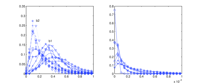
Figure 8: $x$-axis 25cm units/year ($ie$, rate multiplied by cell side length), $y$-axis frequency. (Left) the posterior distributions of migration rate $\beta_{1}$ (solid, ‘b1’) and $\beta_{2}$ (dashed, ‘b2’) in six independent single-phase onset-field models with the $A$ and $B$ hyperprior parameters of Equation (8) given by $(A,B)=(10,1)$ (no symbol), $(A,B)=(20,2)$ (+), $(A,B)=(5,0.5)$ (triangle), $(A,B)=(20,0.5)$ (5-star), $(A,B)=(5,2)$ (6-star) and $(A,B)=(10,1)$ on a $64\times 25$ lattice (circle). Prior simulation at $(A,B)=(10,1)$ has square-symbols. (right) corresponding posterior distributions for $\alpha$.

The prior simulations (left in Fig. 8, colored green, solid and dashed respectively) for $\beta_{1}$ and $\beta_{2}$ coincide. The distributions of the two rates differ in the posterior, and are not shifted by the changing priors with doubled and halved rates. Expansion of the settlement moved more rapidly along than up the beach. The immigration rate is more sensitive to the prior within the range considered.

In order to measure support for spread from a single centre, we count the number of arrival-events,

$$V(\phi)=\sum_{c=1}^{C}\mathbb{I}_{\phi_{c}>\phi_{c^{\prime}}\forall c^{\prime}\in{\mathcal{N}}(c)}$$

in a field. For example, the prior sample in Fig. 3 has $V=2$ arrivals. The posterior to prior odds for $V=1$ in a run with $A=10$ and $B=1$ are greater than one and the odds decline steadily with increasing $V$, so the data push the distribution of $V$ towards fewer arrival events. Our analysis of the model with hyper-prior parameters $(A,B)=(10,1)$ on a $64\times 25$-cell lattice gave essentially identical results. The Bayes factor for $V=1$ against $V=2$ is only slightly greater than one. Very small peaks mask the big picture of Fig. 7. Supporting figures are presented in the Supplementary material.

We have checked that the effects we see are not imposed by the prior distributions we are using. We made a single run with the lattice size doubled to $64\times 25$ on the same region. Results for the default parameter values $A=10$, $B=1$ were very similar to those above (see Supplement). We simulated synthetic data under the single-phase model of Section 4 and fit it with the single-phase onset field model. We do not detect a settlement process where there is none. There is no threshold that splits the cells at $p^{*}=0.8$, that is, one of the green or blue sets is empty for each threshold $T^{*}$. Also, the posterior to prior odds are flat with increasing $V$. Supporting figures are presented in the Supplementary material.

7 Recovering phase structure without spatial structure

We now extend our analysis to the case where the number of phases, and the assignment of specimen to phases, is not known. In this section we make a purely temporal change-point analysis for the unknown piecewise-constant dated-specimen deposition rate.

7.1 Prior model for assignments of specimens to phases

The number of phases $M$, and the map ${\bf m}$ from data index to phase, are now random variables. For $m=1,2,\dots,M$, let $K_{m}({\bf m})={\rm card\,}\{i:{\bf m}(i)=m,i=1,2\dots,K\}$ give the number of dates in the $m$’th phase, and

$$p_{m}(\lambda_{\theta},\psi)=\frac{\lambda_{\theta,m}(\psi_{m}-\psi_{m-1})}{\sum_{m^{\prime}=1}^{M}\lambda_{\theta,m^{\prime}}(\psi_{m^{\prime}}-\psi_{m^{\prime}-1})}.$$

give the probability for specimen $i$ to be assigned to phase ${\bf m}(i)=m$. The prior probability for assignment ${\bf m}$ is a function of ratios of the unknown dated-specimen deposition rates $\lambda_{1},\lambda_{2},\dots,\lambda_{M}$,

$$p({\bf m}|\lambda_{\theta},\psi)=\prod_{m=1}^{M}p_{m}(\lambda_{\theta},\psi)^{K_{m}({\bf m})}$$ (11)

The right hand side of Equation (11) has a multinomial form, without the $K!/\prod_{m}K_{m}!$ factor, because the left hand side is the probability for an assignment ${\bf m}$ of distinct specimen to phases and there are $\prod_{m}K_{m}!/K!$ such assignments. The posterior distribution is now

$$p(M,\psi,\lambda_{\theta},{\bf m},\theta|y)\propto\ell(\theta;y)p(M,\psi,\lambda_{\theta},{\bf m},\theta),$$ (12)

with

$$p(M,\psi,\lambda_{\theta},{\bf m},\theta)=p(M)p(\psi|M)p(\lambda_{\theta}|M)p({\bf m}|\lambda_{\theta},\psi)p(\theta|\psi,{\bf m}).$$

If we condition on $M$ and ${\bf m}$ in Equation (12) we get Equation (3). Of these factors, $p(\theta|\psi,{\bf m})$ and $p(\psi|M)$ are given by Equations (1) and (2) and $p({\bf m}|\lambda_{\theta},\psi)$ in Equation (11). The prior distribution of $M$ (in fact $M-1$, the number of phase boundaries between onset and ending) is Poisson. If we took our prior straight from the deposition-process $\Lambda_{\Psi}$ of Section 4 we would have $M-1\sim\mbox{Poisson}(\lambda_{\psi}(\psi_{M}-\psi_{0}))$. In fact we take $M-1$ Poisson distributed, but fix the mean at $\log(2)$ so that the prior probability that $M=1$ is equal to one half.

Our prior for the dated-specimen deposition rates $\Lambda_{\theta}|M$ is $\lambda_{\theta,m}\sim\mbox{Exp}(1)$ for $m=1,2,\dots,M$. The common scale of the rates is irrelevant as the rate-prior is important only insofar as it decides the prior for the phase allocation probabilities $(p_{1},p_{2},\dots,p_{M})|M$. In our setup, for given $\psi$, dated specimens are a priori more likely to belong to long-lasting phases. When $\psi_{m}-\psi_{m-1}$ are equal for $m=1,2,\dots,M$, we get $(p_{1},p_{2},\dots,p_{M})|\psi\sim\mbox{Dirichelet}(1,1,\dots,1)$. Simulation of the prior shows that, allowing for variation in both $\psi$ and $\lambda_{\theta}$, $(p_{1},p_{2},\dots,p_{M})|M\sim\mbox{Dirichelet}(1/2,1/2,\dots,1/2)$ is a good approximation, for at least $M\lesssim 10$. In the supplement we show that, if we accept this Dirichelet approximation, then the array of numbers of dates in phases, $(K_{1},K_{2},\dots,K_{M})|M$, has a multivariate Polya distribution,

$$p(K_{1},K_{2},\dots,K_{M}|M)\simeq\frac{K!}{\prod_{m=1}^{M}K_{m}!}\frac{\Gamma(M/2)}{\Gamma(K+M/2)}\prod_{m=1}^{M}\frac{\Gamma(K_{m}+1/2)}{\sqrt{\pi}}.$$

Mosimann (1962) gives the moments. The mean is ${\sf E}(K_{m})=K/M$, as we expect. The covariance matrix is a scalar multiple of the covariance matrix of a $\mbox{Multinomial}(1/M,\dots,1/M)$ array and the two distributions have equal correlation matrices. We conclude that the simple choice $\lambda_{\theta,m}\sim\mbox{Exp}(1)$ seems to lead to no unacceptable marginal prior distributions, and other aspects of the prior framework are motivated by the deposition-model framework.

7.2 Estimated phase structure for the Bourewa and Stud Creek data sets

We fit the random phase structure model of Section 7.1 using MCMC. We extend the updates of Nicholls and Jones (2001) to include moves to add and delete phase boundaries, and to move specimen between phases (by varying a specimen age or a phase boundary age). When we add a phase boundary into an existing phase, the state dimension increases by two, as we need a deposition rate for the new phase. We have the Metropolis Hastings Green setup for MCMC in something very like the original variable-dimension application of Green (1995).

7.2.1 Bourewa

When we fit this model to the Bourewa data, we are ignoring spatial structure. The posterior mode has 2 phases. When we plot the locations of specimens assigned in the mode to phases one to three on separate graphs, we get a picture which resembles Fig. 10. The plot is omitted, for brevity, and because it is misleading, as we now explain.

The analysis seems to show expansion from a centre, with the distribution in specimen locations spreading out as we move from phase to phase forwards in time. Do we need an onset-field analysis if the phase assignment model shows such a clear effect? First, and most important, central pits have more dates, so they may display more early dates. Secondly, if the settlement did expand, and the specimen are selected for dating uniformly in space and time, then we get more dates when the settlement is larger, and we get a good fit to the rate with a staircase of physically spurious phases.

7.2.2 Stud Creek

The phase-assignment analysis is useful for measuring support for alternative temporal phase-structure models, as we now illustrate.

Stud creek is a small stream system in far western New South Wales, Australia. The area was excavated between 1996 and 1998, and the remains of 72 hearths were recorded, of which 28 yielded one dated specimen each. These data are reported in Holdaway et al. (2002) and Holdaway et al. (2008), who argue that, in our terms, the dated hearths are a random sample from the population of previously buried hearths in the study area. Although there has been some localized erosion, hearths are scattered over a wide area, with hearths of markedly different ages located adjacent to one another. Their likelihood is graphed in Fig. 9.

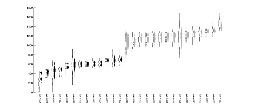
Figure 9: (black outline) likelihoods for the Stud Creek data of Holdaway et al. (2002); (black, gray filled) marginal posterior distributions of ages shaded by phase assignment (black) phase 1, and (gray) phase 3 and conditioned on that assignment. (y-axis) years BP, (x-axis) specimen label per Holdaway et al. (2002).

The archaeologists conject that the site was in use in two separate phases, with a hiatus associated with climate change. This question is answered in Holdaway et al. (2002). We use these data to illustrate our methods for recovering archaeological phase structure. Exploratory analysis by the authors of Holdaway et al. (2002) showed no spatial structure in the specimen ages.

In order to estimate the phase structure of the Stud creek data we fit the phase-structure model of this section to the data (with limits $L=0$ and $U=2000$ years BP). When we fit a phase structured model to determine phase, we are making a model comparison over phase models in a discrete set. The prior distribution over phase models allows any number $M$ of phases, and an arbitrary assignment ${\bf m}$ of specimen to phases. In the past, model comparison of this kind has been made for a very small number of alternative models, typically, two. For example, Jones and Nicholls (2002) estimate Bayes factors in order to weigh support for two models of a small radiocarbon date data set with ($M=6,{\bf m}=(1,2,3,4,5,5,6)$) and without ($M=1,{\bf m}=(1,1,1,1,1,1,1)$) stratigraphic phases, from $K=7$ dated specimen. For the Stud creek data, Holdaway et al. (2002) compare model $A=\{M=3,{\bf m}=(1\times 13,3\times 15)\}$ with model $B=\{M=1,{\bf m}=(1\times 28)\}$ for the $K=28$ stud creek dates. Model A has an empty phase (phase $2$) for hearth construction explaining the obvious step in Fig. 9. We will make two model comparisons, between models $A$ and $B$, and between models $A^{\prime}=\{M=3\}$ and $B^{\prime}=\{M=1\}$. The $A^{\prime}\ v.\ B^{\prime}$ comparison weighs the evidence for three phases, as opposed to one, without specifying which specimens are in which phase. The models in the $A\ v.\ B$ comparison specify specimens’ phase assignments.

We begin with the $A^{\prime}\ v.\ B^{\prime}$ comparison. The Bayes factor is the ratio of the posterior to prior odds ratios,

$${\mathcal{B}}(A^{\prime},B^{\prime})=\frac{\Pr(A^{\prime}|y)}{\Pr(B^{\prime}|y)}\frac{\Pr(B^{\prime})}{\Pr(A^{\prime})}.$$

We estimate $\widehat{\Pr(A^{\prime}|y)}\simeq 0.20$ and $\widehat{\Pr(B^{\prime}|y)}\simeq 0.41$ as the proportion of states $X_{t}$ with $M=3$ and $M=1$ phases respectively, in MCMC simulations with $X^{(t)}=(M^{(t)},\psi^{(t)},\lambda_{\theta}^{(t)},{\bf m}^{(t)},\theta^{(t)})$ for $t=1,2,\dots,T$ and convergence $X^{(t)}\stackrel{{\scriptstyle D}}{{\rightarrow}}p(M,\psi,\lambda_{\theta},{\bf m},\theta|y)$ to the posterior. The quantities $\Pr(A^{\prime})\simeq 0.12$ and $\Pr(B^{\prime})=0.5$ are $\mbox{Poisson}(M-1;\log(2))$. We find ${\mathcal{B}}(A^{\prime},B^{\prime})\simeq 2.03$ so there is very mild support for 3 phases over one. The reason for this weak positive support, is that model $A^{\prime}$ is a large class of models, including many very improbable assignments ${\bf m}$ of specimens to its three phases. The mean likelihood in the $A^{\prime}$-prior is lowered by these models.

Since there is just one way to assign $K$ specimen to $M=1$ phases, $B=B^{\prime}$ and we have $\widehat{\Pr(B|y)}\simeq 0.41$ and $\Pr(B)=0.5$ as before. The posterior probability for $A$ was large enough to estimate simply, at $\widehat{\Pr(A|y)}\simeq 0.08$. The prior for $A$ is $\Pr(M,{\bf m})=\Pr({\bf m}|M)\Pr(M)$ with $\Pr(M=3)\simeq 0.12$ and $P({\bf m}|M)$ calculated in the supplement as $\Pr({\bf m}|M)\simeq 10^{-10}$. The Bayes factor is then ${\mathcal{B}}(A,B)\simeq 8\times 10^{9}$ so the support for $A$ over $B$ is overwhelming. The red and blue histograms in Fig. 9 show the posterior distribution for the hearth ages, conditioned on model A, whilst the colors show the maximum a posteriori phase assignment.

Inference for $M,{\bf m}$ is useful for exploratory analysis. When we fit the Stud-creek data, in the $(A^{\prime},B^{\prime})$-analysis, the hiatus model $A$ is thrown up as worth closer inspection in a search over many models. We looked at other priors on $M$ and ${\bf m}$: one of these is discussed further in the supplement.

8 Fitting the onset-field for multiple phases

If a settlement forms, spreads, and from time to time undergoes dramatic changes in character, so that the deposition at all settled locations moves into a new phase, we should fit a model with local deposition switched on by the spreading onset-field, cut across with an unknown number $M$ of site-wide phase boundaries. This is the onset-field model described in Section 5.3 augmented with the prior weighting for $M$, the relative deposition rates $\lambda_{\theta}=(\lambda_{\theta,1},\lambda_{\theta,2},\dots,\lambda_{\theta,M})$ and the specimen to phase map ${\bf m}$ described in Section 7. The posterior density is

$$p(\alpha,\beta,\phi,M,\psi,\lambda_{\theta},{\bf m},\theta|y)\propto\ell(\theta;y)p(\alpha,\beta,\phi,M,\psi,\lambda_{\theta},{\bf m},\theta),$$

with

$$p(\alpha,\beta,\phi,M,\psi,\lambda_{\theta},{\bf m},\theta)=p(\alpha,\beta)p(M)p(\psi|M)p(\lambda_{\theta}|M)p(\phi|\psi,\alpha,\beta)p({\bf m}|\lambda_{\theta},\psi,\phi)p(\theta|\psi,{\bf m},\phi).$$

In order to clarify the state, we explain how to simulate the prior. We simulate $M\sim\mbox{Poisson}(\log(2))$ and $\psi$ according to Equation (1). The onset field is simulated using the algorithm in Section 5.1, with $\alpha$ and the two components of $\beta$ independent and distributed as Equation (8). These steps are repeated until $\max(\phi)\geq\psi_{0}$. We have now to assign the specimen to phase map ${\bf m}$ and specimen ages $\theta_{1},\theta_{2},\dots,\theta_{K}$. The probability, $p_{m,i}$ say, for specimen $i$ to be assigned to phase $m$ depends now on the local onset field, since the deposition rate at a pit before onset is zero. Deposition in phase $m$ does not occur at pit $h$ at ages before $\phi_{c(x_{h})}$. Let

$$\Delta_{m,h}=\max(0,(\min(\phi_{{\bf c}(x_{h})},\psi_{m})-\psi_{m-1}))$$

give the span of deposition in phase $m$ at pit $h$. The conditional single-specimen phase-assignment probability is

$$p_{m,i}=\frac{\lambda_{\theta,m}\Delta_{m,{\bf h}(i)}}{\sum_{m^{\prime}=1}^{M}\lambda_{\theta,m^{\prime}}\Delta_{m^{\prime},{\bf h}(i)}}$$

independently for each $i=1,2,\dots,K$ and the conditional probability for any particular phase assignment ${\bf m}$ is

$$p({\bf m}|\lambda_{\theta},\psi)=\prod_{i=1}^{K}p_{{\bf m}(i),i}(\lambda_{\theta},\psi,\phi).$$

Finally, the unknown true specimen ages $\theta_{i},\ i=1,2,\dots,K$ are uniformly distributed in $\psi_{{\bf m}(i)-1}<\theta_{i}<\min(\psi_{m},\phi_{{\bf c}(i)})$ as before. The MCMC simulation of the posterior $p(\alpha,\beta,\phi,M,\psi,\lambda_{\theta},{\bf m},\theta|y)$ combines the MCMC updates of Sections 6 and 7.2. Each MCMC simulation involving onset-fields takes at least 24 hours to run.

The posterior onset-field distribution we obtain fitting this second random-phase model is very similar to the distribution we had in the single phase onset-field model. The figures corresponding to Figures 5, 6 and Figure 7 appear in the supplementary material.

The modal number of phases is one. However, the prior weights in favor of a single phase. We can estimate marginal likelihoods,

$$e_{m}=\Pr(M=m|y)/\Pr(M=m)$$

for $M=m$ phases, averaged over all other parameters. The ratio $e_{m_{1}}/e_{m_{2}}$ is the Bayes factor for the model comparison of $M=m_{1}$ against $M=m_{2}$ phases. We find $\hat{e}_{1}\simeq 0.8$, $\hat{e}_{2}\simeq 1$ and $\hat{e}_{3}\simeq 1.3$, so the single phase model of Section 6 is not contradicted.

In order to visualise the settlement directly on the data, we look at the distribution of dates when there are three phases (supported by the largest reliably estimated marginal likelihood). The scatter of the specimens in each phase is shown in Fig. 10. The scatter plots shows a clear spreading trend as we move from phase to phase.

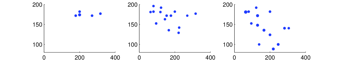
Figure 10: The scatter of specimen by phase, in the posterior mode assignment ${\bf m}$ conditional on three phases, in a random-phase model with onset-field. (left) Phase 3 (middle) Phase 2 (right) Phase 1. Axes are specimen excavation coordinates. Time increases left to right from phase 3 to phase 1. Point-size is proportional to posterior probability for the given phase assignment.

9 Conclusions

We have fitted four models to the data: a simple single-phase model without spatial structure (Section 4), a single-phase model with an onset field (Section 6), a random-phase model with no spatial structure (7.2), and a random phase model with onset-field (Section 8). The single-phase onset-field (second model) models the unknown specimen dates at each pit as uniformly distributed in time between the local onset and the end-of-deposition event. The single-phase model without onset-field (first model) applies too much shrinkage to the earliest dates, as the total deposition rate in a spreading settlement is not initially large. This is visible in Fig. 4 where the single-phase estimate for $\psi_{M}$ is shifted by 200 years towards the present. The single-phase onset-field model estimate 3000-3200 BP will be more reliable. The onset-field priors do not overwhelm the data.

In the random-phase model (third model), phases are the pieces of the piece-wise constant specimen-age intensity. Like the first model, this model treats the site as a single spatially unstructured pit, ignoring variations in the intensity which might be due to onset-time varying from place to place. It will detect the low initial deposition rate and not over-shrink. However, it is unlikely that the phases recovered by the random phase model correspond to physically distinct phases, in the archaeological sense. The evidence for phases is variation in the intensity of the dated-specimen ages. Such variation might be caused by any one of many time-varying selection processes which thin dateable material down to dated specimen. However, the random phase model does provide, at least heuristically, for rate variation, in the spirit of Blaauw and Christen (2005), who model the age-depth relation with a variable number of accumulation sections, and Karlsberg (2006), who parameterises rate variation within a fixed number of phases. The Stud Creek hiatus example has the unusual property that confounding processes may be absent.

The random-phase onset-field model (fourth model) adapts to heterogeneity in spatial and temporal deposition rates. It is rather complex. However, it functions as a model-mispecification check on the constant-rate hypothesis of the simpler single-phase onset-field model, which it supports, as it allows a single phase.

Our analysis (Fig. 4) shows that the human-associated deposition did not commence at each pit location at the same time. The posterior mean onset field Fig. 6 shows the pattern of expansion from a central location in the onset of deposition at Bourewa. Ancient human settlement generating dated specimen begins in the area between pits ‘1’,‘4’ and ‘X6’ and takes some 150-200 years to spread some 40-50 meters along the beach to pits ‘2’, ‘A1A’ and ‘A1D’.

References

- Ammerman and Cavalli-Sforza (1971) Ammerman, A. and L. Cavalli-Sforza (1971). Measuring the rate of spread of early farming in Europe. Man 6, 674–688.
- Bayliss et al. (2007) Bayliss, A., C. B. Ramsey, J. van der Plicht, and A. Whittle (2007). Bradshaw and Bayes: Towards a timetable for the Neolithic. Cambridge Archaeological Journal 17(1 (suppl.)), 1–28.
- Blaauw and Christen (2005) Blaauw, M. and J. Christen (2005). Radiocarbon peat chronologies and environmental change. Appl. Statist. 54, 805–816.