Species assembly in model ecosystems, II: Results of the assembly process.

Abstract

In the companion paper of this set (Capitán and Cuesta, 2010) we have developed a full analytical treatment of the model of species assembly introduced in Capitán et al. (2009). This model is based on the construction of an assembly graph containing all viable configurations of the community, and the definition of a Markov chain whose transitions are the transformations of communities by new species invasions. In the present paper we provide an exhaustive numerical analysis of the model, describing the average time to the recurrent state, the statistics of avalanches, and the dependence of the results on the amount of available resource. Our results are based on the fact that the Markov chain provides an asymptotic probability distribution for the recurrent states, which can be used to obtain averages of observables as well as the time variation of these magnitudes during succession, in an exact manner. Since the absorption times into the recurrent set are found to be comparable to the size of the system, the end state is quickly reached (in units of the invasion time). Thus, the final ecosystem can be regarded as a fluctuating complex system where species are continually replaced by newcomers without ever leaving the set of recurrent patterns. The assembly graph is dominated by pathways in which most invasions are accepted, triggering small extinction avalanches. Through the assembly process, communities become less resilient (e.g., have a higher return time to equilibrium) but become more robust in terms of resistance against new invasions.

1 Introduction

Understanding the mechanisms leading to species assembly in ecological communities is a challenging issue. In particular, assembly models have been used to understand the observation that natural communities are both complex and stable (McCann, 2000; Dunne, 2006).

Assembly models try to mimic the sequential arriving of rare species (invaders) to which natural communities are subjected. Standard assembly models (Drake, 1990; Law and Morton, 1993, 1996) use “species pools” as (finite) sets of potential invaders. Pools are usually defined by labeling species according to some niche variable (usually a species trait like body size) and then drawing randomly their interactions from predetermined probability distributions (Law and Morton, 1996). Sequential invaders of any given resident community are selected from the pool at each invasion attempt, and the resulting community after the invasion can be determined according to some population dynamics. For models using Lotka-Volterra equations, the permanence (Hofbauer and Sigmund, 1998) of the invaded community is a suitable criterion which determines the same final community as the numerical integration of the equations (Morton et al., 1996).

The most remarkable results of previous assembly models are: (i) a final end state is eventually reached, which can be either a single community or a cycle involving several communities (Morton and Law, 1997), (ii) average species richness (complexity) increases with successional time (Post and Pimm, 1983; Drake, 1990; Law and Morton, 1996), and (iii) stability, understood as resistance against invasions, also increases with time (Case, 1990; Law and Morton, 1996; Morton and Law, 1997). Thus assembly models conform a well-founded theoretical framework that provides a positive relationship between stability and complexity in model communities.

In a previous paper (Capitán et al., 2009) we have provided a picture of the assembly process of an ecosystem as a Markov chain evolving in a certain configuration space. This space is made of all viable communities for a given set of parameters (resource saturation, interspecific competition, consumption rates…). The invasion process by a new species induces transitions as a result of the perturbations created in the community by the newcomer. The process drives the community to an end state resistant to invasions. For some parameter values this end state is just a single uninvadable community. For the remaining values, the end state is formed by a set of communities with equal number of trophic levels and similar number of species per level, which transform into each other as a result of new invasions. In this set, communities can always be invaded but they never abandon the set. These complex end states are a generalization of the end cycles found in previous assembly models (Morton and Law, 1997), and the fact that they had not been observed so far is probably due to limitations in the pool of invaders of these previous models. In the preceding paper (Capitán and Cuesta, 2010) we have shown that the existence of these complex end states is a result of a top predator attempting to invade a community when its establishment is not allowed by the parameters of the model.

Our model recovers the main findings of previous assembly models (Post and Pimm, 1983; Drake, 1990; Case, 1990; Law and Morton, 1993, 1996), such as the resistance of end states against invasions, or the increase of complexity (biodiversity) along the assembly (Capitán et al., 2009). Its main virtue is therefore being sufficiently simple so as to allow mapping out all assembly pathways, thus providing a global picture of the assembly process.

Despite recovering the above similar results, there are important differences between our work and early models. First, the niche variable in our model is simply the trophic level (Capitán et al., 2009), which renders our species pool infinite (in contrast to most previous models; but see Post and Pimm (1983) for an exception). However, interactions in the pool are averaged over each trophic level under a species symmetry assumption (Capitán and Cuesta, 2010), which decreases substantially the number of different assembly pathways. Second, in our model the permanence of the final community is guaranteed because we are able to show that equilibrium communities are globally stable (Hofbauer and Sigmund, 1998) under the assumption of neutrality within each trophic level. And third, in standard assembly models magnitudes are averaged over a set of stochastic realizations of the process of sequential invasions, where invaders are randomly chosen from the species in the pool not yet present in the community. Since we are able to map out all the invasion pathways for this model, we do not need to resort to average magnitudes over realizations but we can calculate them exactly (Capitán et al., 2009). Even for our simple model, the number of possible pathways is too high to be accounted by through simulation [see details in Capitán et al. (2009)]. This is one of the main advantages of our model with respect to former ones, which in turn allows us to establish its independence on history. The uniqueness of the end state for these kind of models was not proven until now, although it was already found that most of the simulated assembly sequences led to a single set of final communities (Morton and Law, 1997).

In the first paper of this suite (Capitán and Cuesta, 2010) we have performed a detailed analysis of the analytical properties of the Lotka-Volterra population dynamics underlying our assembly model, as well as the stability properties of the interior equilibria from the dynamic point of view. Our communities represent a mean-field version of trophic networks: the feeding relations are assumed to take place only between contiguous trophic levels and the strength of each interaction is averaged to a uniform value. This assumption of symmetry allowed us to simplify the differential equations, showing that in our model the set of species numbers at each level $\{s_{\ell}\}_{\ell=1}^{L}$ is enough to determine the equilibrium densities and the dynamics of a community with $L$ trophic levels.

The present paper presents new results of the assembly process ranging from structural properties of the building of stable communities to dynamical properties of the stochastic invasion process. The transition matrix associated to the chain allows us to define a stationary distribution of probabilities over the assembly graph. We will use that distribution to calculate averages of biologically relevant observables in the ecosystem, like the average number of species, the total population density, etc., and even to obtain distributions of certain magnitudes like the fraction of extinct species after a destructive invasion. But this is not the only advantage of our approach. The transition matrix also provides the time evolution of the probability, so the dependence in time of any magnitude can be obtained exactly. Due to its simplifications, the model reduces the number of possible communities to a finite graph. Once we have that graph, the theory of finite Markov chains can be exploited to obtain the dynamical properties of the assembly process.

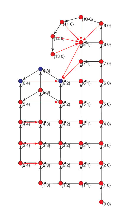
Figure 1: (Color online) Assembly graph obtained for a value of the resource saturation $R=80$. It is made of $39$ communities (nodes), each of them with either one or two trophic levels. Transitions shown with a black arrow indicate that the invasion is accepted, and those with a red arrow refer to a rearrangement in the resulting community after the invasion. Transient nodes are filled in red, and recurrent nodes are filled in dark blue. In this case, the final end state of recurrent communities comprises 3 communities forming an end cycle like those found by Morton and Law (1997). Labels of each node show the species numbers $\{s_{1},s_{2}\}$ of each trophic level in the community. (For the choice of parameters see Section 3.2.)

The paper has been organized as follows. In Section 2 we revisit the definition of the Markov chain associated to the assembly process and show that all communities can be classified into transient or recurrent. Section 3 is devoted to discuss the main statistical results that can be obtained for our model, for instance, the asymptotic distribution within the complex end states (Section 3.1), the dependence of averages upon variation of the resource saturation (Section 3.2), the dependence of the results upon variation of the parameters of the model (Section 3.3), the average time to reach the end state (Section 3.4), the statistics of avalanches of extinctions caused by invasions (Section 3.5) or the variation of biologically relevant averages with successional time (Section 3.6). We finally discuss our findings and their implications in Section 4.

2 The assembly process as a Markov chain

Let us start with a detailed description of the Markov chain associated to our assembly model In the first paper of this suite (Capitán and Cuesta, 2010) we showed that, solving the linear system that defines the interior equilibrium point of the Lotka-Volterra equations (i.e., the system obtained by equating to zero the per-capita population growth rates $\dot{n}_{i}/n_{i}$, with $i$ running over the set of all species) we can determine all viable communities (i.e., those whose population densities are above a certain extinction threshold $n_{c}>0$) that are compatible with a given set of parameters. Although in principle the population model allows for infinitely many species at each level, it turns out that the set of viable communities is finite. This is a consequence of the existence of the extinction threshold, that precludes the appearance of arbitrarily small populations (an unrealistic feature of deterministic population dynamics models). There is another limitation due to the finite amount of abiotic resource that maintains our model communities. In our previous work we modeled this resource with a linear functional response with a saturation value $R$ (Capitán et al., 2009; Capitán and Cuesta, 2010). $R$ accounts for the amount of resource that would be reached in the absence of consumers. On the one hand there is a maximum number of levels allowed for a given resource saturation $R$ (Capitán and Cuesta, 2010); on the other hand population densities at each level decrease as $1/s_{\ell}$, with $s_{\ell}$ the number of species in that level (Capitán and Cuesta, 2010), so we can have populations infinitely close to zero. Therefore, the existence of the extinction threshold renders the set of communities under consideration finite, and then the associated Markov chain has a finite number of states. Besides this being a more realistic description of an ecosystem, it also drastically simplifies the analysis of the assembly process.

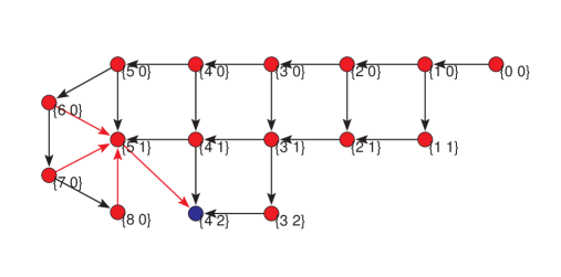
Figure 2: (Color online) Same as Figure 1 for $R=50$. The total number of communities in this graph is $16$, and they have up to $2$ trophic levels. An end state with a single community (with occupancies $\{4,2\}$) is reached in this case.

Thus for any choices of parameters there is a finite set of viable communities —that we denote by $\mathcal{F}$. There will be a link from community $i$ to community $j$ of the set $\mathcal{F}$ provided the former is transformed into the latter as a result of an invasion. Invasions are assumed to occur at a uniform rate $\xi$. We assume that the typical dynamical time is much smaller than $\xi^{-1}$, the mean time between invasions, so that communities are always at equilibrium when an invasion occurs [for the validity of this assumption see the discussion in Capitán and Cuesta (2010)] The population of the invader is assumed as small as possible, i.e. equal to $n_{c}$ (Roughgarden, 1974; Turelli, 1981).

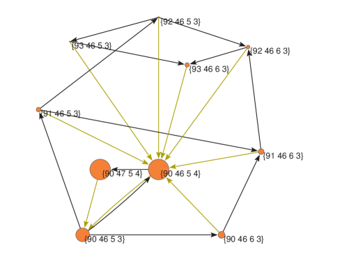
(a) (b)

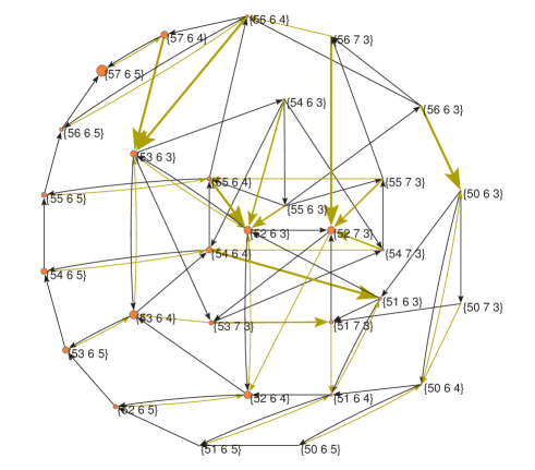
Figure 3: (Color online) Graphs of the recurrent subset for values of the resource saturation $R=990$ (a) and $R=390$ (b) (other parameters are set as in Figures 1 and 2). The first graph contains 10 communities with 4 trophic levels, whereas the second has 30 communities with 3 levels. For a graphical representation of a recurrent subset more complex than these see Capitán et al. (2009). All the communities in both cases have three trophic levels. The diameter of the nodes is proportional to its asymptotic probability. Black arrows show accepted invasions and yellow ones those causing a reconfiguration (the thickness of each line is proportional to the relative number of extinct species). Labels indicate the number of species in each trophic level.

Consider a community $i\in\mathcal{F}$, with $L$ trophic levels, at its equilibrium point. Potential invaders are species of level $\ell=1,\dots,L+1$ (species of higher levels would not be able to feed from the existing levels). We randomly choose $\ell$ and introduce a new species at level $\ell$ of the community $i$. The extended community will evolve to the interior equilibrium corresponding to the new number of species $s_{\ell}+1$ at level $\ell$ (Capitán and Cuesta, 2010). If this equilibrium is viable, then the invader is accepted in the resident community. The new community $j$ will also be in $\mathcal{F}$ and a directed link will go from $i$ to $j$. If the new equilibrium is not viable then we apply the procedure discussed in Capitán and Cuesta (2010) to determine what is the sequence of extinctions until the community becomes viable. Two things can happen: either the first level to fall below the extinction threshold is the invaded one, or it is another one. In the former case the invader is simply rejected and the community remains unaltered; in the latter, the extinction sequence will lead to a new community $k\in\mathcal{F}$, and a link will go from $i$ to $k$.

The assembly graph, $\mathcal{G}$, is defined as the connected component containing the empty community, $\varnothing$, of the directed graph whose nodes are the elements of $\mathcal{F}$ and whose links are the transitions obtained by the invasion process just described. Obviously, the way to construct $\mathcal{G}$ is to start off from $\varnothing$, and proceed by attempting all possible invasions for every community reached along the assembly process [see Figures 1 and 2 for a graphic representation of simple assembly graphs, for a larger value of $R$ see Figure 1 in Capitán et al. (2009)]. The exhaustive characterization of the set of nodes in $\mathcal{G}$ is a bit demanding. For example, the storage of all the communities appearing along the process has been carried out by using a binary tree (Knuth, 1997), by exploiting the mapping between any configuration $\{s_{\ell}\}_{\ell=1}^{L}$ and a binary number (we simply concatenate the binary representations of each species number $s_{\ell}$ to form a branch of the binary tree). Despite this, we have been able to analyze graphs with around $10^{6}$ communities within.

The connection of the species assembly process with a Markov chain on the graph $\mathcal{G}$ amounts to assigning certain transition probabilities to each link of the assembly graph. We define these probabilities in a simple way. Invaders arrive at each community at a constant rate $\xi$, independent of the level of invasion, and the stochastic process is updated in discrete time (each time unit is the average time elapsed between consecutive invasions). Thus, if $i$ and $j$ are two nodes of $\mathcal{G}$ connected by a link, we assign it the transition probability

$$P_{ij}=\delta_{ij}+\xi Q_{ij},$$ (1)

where $\delta_{ij}=1$ if $i=j$ and $0$ otherwise. The matrix elements $Q_{ij}$ are given by

$$Q_{ij}=\frac{n_{ij}}{L+1},\quad i\neq j,\qquad Q_{ii}=-\sum_{j\neq i}Q_{ij},$$ (2)

where $n_{ij}$ is the number of different invasions of $i$ that lead to $j$ and $L+1$ is the number of different invasions of $i$, provided it has $L$ trophic levels. Therefore, the probability of the transition $i\rightarrow j$ between different communities is proportional to the relative frequency of the transition among all the possible transitions starting from $i$, the invasion rate being the proportionality constant. The diagonal of $Q$ is chosen so that $P=(P_{ij})$ is a stochastic matrix.

Since the diagonal elements of the transition matrix $P$ are non-zero, the Markov chain can not be periodic (Karlin and Taylor, 1975). As the set of viable ecosystems $\mathcal{F}$ is finite, $P$ defines the transition matrix of a finite, aperiodic, Markov chain. The states of one such chain are either transient or recurrent (Karlin and Taylor, 1975). There can be one or several subsets of recurrent states, the chain being ergodic in each of them. Every recurrent subset is a different end state of the assembly process. The end state of an ecosystem will be history-dependent only if there are at least two such recurrent subsets. Ergodicity implies that there is a stationary probability distribution on the states of these subsets which determines the frequency with which the process visits each of them. [For a full account on Markov chains see e.g. Karlin and Taylor (1975)]. Our model only exhibits a unique recurrent set for any given set of parameter values (Capitán et al., 2009).

$parameter$	$value$	$interpretation$
$R$	$10\leq R\leq 1700$	Saturation value, in the absence of predation, of the abiotic resource abundance
$\alpha$	$1$	Average mortality rate of consumers
$\gamma_{-}$	$5$	Average rate of decrease in preys population caused by their being predated
$\gamma_{+}$	$0.5$	Average rate of increase in predators population due to feeding
$\rho$	$0\leq\rho\leq 1$	Relative magnitude between intra– and interspecific competition
$n_{c}$	$1$	Extinction threshold

Table 1: Summary of parameters of the model and ecological meaning of each one of them.

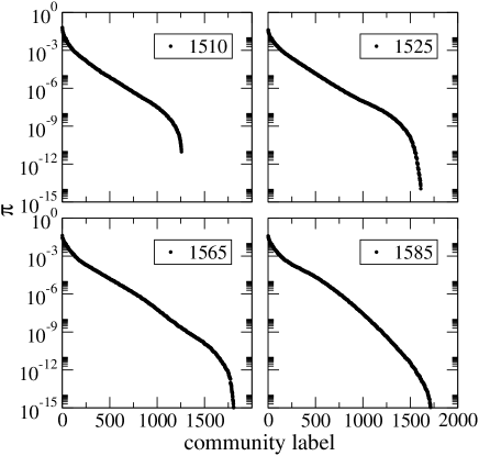
Figure 4: Distribution of asymptotic probabilities $\pi$ within each recurrent set, for several values of $R$. Communities are labelled in decreasing order of probability. The distributions look exponential with a cutoff.

This concludes the definition of the Markov model for the assembly process. As we are able to compute the whole transition matrix $P$, we have a complete and exact characterization of the assembly process. In particular, by selecting an initial state for the Markov chain (in our case the process always starts off from $\varnothing$), we can obtain the evolution of any magnitude —numerically but exactly— without resorting to taking averages over realizations of the process. In the following section we will discuss in detail the results that can be obtained from the analysis of the Markov chain [a brief account of which were reported in Capitán et al. (2009)].

3 Results

3.1 Asymptotic distribution

To separate transient and recurrent states, we have applied an algorithm provided by Xie and Beerel (1998). Notice that the characterization of transient and recurrent states in a finite chain depends only on the graph, not on the transition probabilities. Only one subset of recurrent states was found for each set of parameters. Let $\mathcal{R}$ denote the subgraph of $\mathcal{G}$ formed by this ergodic set. Figure 3 shows two examples of these subgraphs. The particular transition probabilities assigned to each link would determine the asymptotic probability distribution within the recurrent set, but not the subset of nodes contained in it.

In order to calculate the asymptotic probability $\pi_{i}$ for a community $i\in\mathcal{G}$, we need to solve the linear system $\pi=\pi P$ (Karlin and Taylor, 1975), in other words, the vector $\pi$ of probabilities is the left eigenvector of the matrix $P$ with eigenvalue 1. Since our graphs are very sparse, standard numerical techniques for solving sparse systems have been applied. The eigenvector is normalized to satisfy the condition $\sum_{i\in\mathcal{R}}\pi_{i}=1$. Obviously, we only need to solve this system for the subgraph corresponding to the recurrent set, since by definition the asymptotic probability $\pi_{i}=0$ for any transient state $i$. Note that our matrix of transition probabilities (1) reduces the condition to be satisfied by $\pi$ to $\pi Q=0$, i.e., $\pi$ is a left eigenvector of $Q$ with eigenvalue $0$. It is worth noticing that neither the asymptotic distribution, nor the recurrent subset depends on the invasion rate.

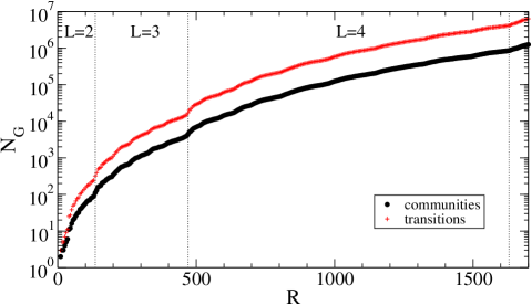
Figure 5: (Color online) Total number of communities (black circles, below) and transitions (red crosses, above) in the Markov chain as a function of the resource saturation $R$.

We can thus obtain a probability distribution for each recurrent set. Having this probability distribution is therefore equivalent to defining a statistical mechanics over the set of viable communities, if we regard $\mathcal{F}$ as the phase space of our system. In Figure 4 we have plotted the histogram of probabilities for several values of the resource saturation $R$ (for these values the number of communities in each set is larger than $10^{3}$). Communities are labelled in decreasing order of probability. These distributions are found to be roughly exponential over several orders of magnitude, this meaning that only a small number of communities (in general very similar to each other) occur with high probability. These are the communities in which it is more likely to find the ecosystem. Nonetheless ergodicity implies that all communities in the end state are visited with non-zero probability. The ecosystem is thus in a complex state, with fluctuating species numbers in each level due to some invasions being accepted and some others causing avalanches of extinctions.

This distribution can be used to calculate the asymptotic average over $\mathcal{R}$ of any relevant magnitude $M_{i}$ defined for every community, like for instance the average number of species, the total population, etc. We just need to evaluate $\langle M\rangle_{\mathcal{R}}=\sum_{i\in\mathcal{R}}\pi_{i}M_{i}$.

3.2 Dependence with the resource saturation

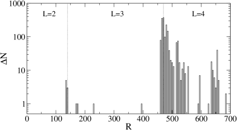
Figure 6: Number of viable states that are not reachable trough invasions starting from the empty community $\varnothing$, $\Delta N=N_{\mathcal{F}}-N_{\mathcal{G}}$. Typically there is an accumulation of these communities in the regions where $R$ allows a top predator in them.

All results presented here have been obtained with a death rate $\alpha=1$, an extinction threshold $n_{c}=1$, an average rate of increase in predators population per predation event $\gamma_{+}=0.5$, and an average decrease in reproduction rate of preys per predation event $\gamma_{-}=5$ (see Capitán and Cuesta (2010) for details on the way these parameters enter the population equations of the model and Table 1 for a brief summary of them). The assumption of $\gamma_{+}\ll\gamma_{-}$ is ecologically sound, because many preys must be consumed to produce a new predator, while loosing one prey requires a single predation event. A common choice for the energy transfer between trophic levels is about 10% (Pimm, 1991). We have checked that the model is robust against variations of these parameters within reasonable bounds.

In most cases we have taken the ratio of direct inter- to intraspecific competition $\rho=0.3$. However, we have explored the effect of this parameter in detail in Section 3.3.

We have obtained all assembly graphs in a range of resource saturations that goes from $R=10$ up to $R=1700$ with increments $\Delta R=5$. No viable community is found below $R=10$. The number of communities $N_{\mathcal{G}}$ in these graphs goes from just one (for $R=10$) up to about $10^{6}$. We have found empirically that both this number and the total number of transitions in each graph grow roughly as $e^{\kappa\sqrt{R}}$, see Figure 5. The maximum number of trophic levels that are allowed up to $R=1700$ is $5$.

We have checked whether the set of communities in the assembly graph is the whole set $\mathcal{F}$. Given the estimation of the resource values that allow a maximum number of levels $L_{\rm max}$ [see Capitán and Cuesta (2010)], we have checked the viability of all possible combinations of species numbers $\{s_{\ell}\}_{\ell=1}^{L_{\rm max}}$ with $L_{\rm max}+1$ levels up to a total number of species $S_{\rm max}$ equal to twice the maximum number of species allowed for that $R$ value. Since there is a huge number of these combinations when $R$ increases, we have checked this up to $R=700$. Figure 6 shows the difference $\Delta N=N_{\mathcal{F}}-N_{\mathcal{G}}$. In nearly all cases the set of communities in the assembly graph is $\mathcal{F}$, but we have found several instances —all of them near the values of $R$ at which new levels arise— in which $\mathcal{F}$ contains communities not reachable through the assembly process, just like in the experiment of Warren et al. (2003). The largest difference is found at $R=470$, where $N_{\mathcal{G}}=4800$ and $\Delta N=375$, so the highest relative difference reaches 8%.

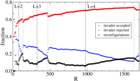
Figure 7: (Color online) Statistics of links corresponding to accepted invasions (red squares), rejected invasions (blue crosses) and invasions that lead to a reconfigured community through an avalanche of extinctions (black circles). Dotted lines correspond to the onsets of acceptance of a new trophic level, and dashed lines to the beginning of the regions of complex end states.

For each $R$ we determined the number of recurrent states of the chain (see Figure 3 in Capitán et al. (2009) for a plot of this number as a function of $R$). We always found a single connected graph, which implies that the end state of the assembly process does not depend on history for this model (Drake, 1990). This is consistent with the results of Morton and Law (1997) as well as the experiments of Warren et al. (2003). There are values of $R$ for which this set consists of a unique absorbing state (or just a few, sometimes forming a cycle), but when $R$ is reaching the values at which a new trophic level appears, the size of this set increases considerably (the largest set found contains around $1800$ communities; a tiny fraction of the whole assembly graph, anyway). After crossing these values the size of the recurrent set drops again down to just one absorbing state. Morton and Law (1997) also obtained complex end states in $6$ out of the $80$ pools they explored, with a number of communities ranging from $6$ to $138$.

(a) (b)  

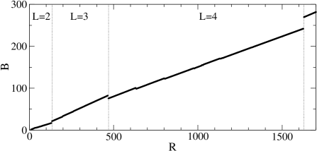
Figure 8: (a) Mean return time in the stationary state vs. resource saturation $R$. The behavior is approximately constant, except for the region of low resources, where the graphs contain less communities and there is more variability. (b) Mean population density of the community vs. $R$.

In Figure 7 we show the fractions of links in the assembly graph corresponding to invasions that are accepted, rejected, or cause a reconfiguration in the system through a sequence of extinctions. The most frequent case is the acceptance of the invader, although there are around 20% of rejections and reconfigurations. We can see an increasing trend to reconfigurations when $R$ corresponds to a complex end state [see Figure 3 in Capitán et al. (2009)]. The invasibility criterion discussed in Capitán and Cuesta (2010) explains why we observe an increasing number of rearranged communities in these regions.

As for the dynamic stability (resilience), we can measure the return time, i.e., the mean time that a perturbed ecosystem needs to restore equilibrium (Pimm and Lawton, 1977), averaged over the probability distribution of the stationary state. It can be obtained as $T_{\rm r}=-\lambda_{\rm max}^{-1}$, where $\lambda_{\rm max}$ is the largest real part of the eigenvalues of the linear stability matrix —which is always negative in our communities since they are globally stable. We observe that this time is roughly independent on the end state, being approximately constant as a function of the resource saturation $R$ (see Figure 8a).

For each end state, regardless on whether it is an absorbing community or a recurrent set, we have calculated another average. In Figure 8b we show the dependence of the total population of a community, $B=\sum_{\ell=1}^{L}s_{\ell}p^{\ell}$, averaged over the recurrent set $\mathcal{R}$, as a function of the resource saturation $R$ ($p^{\ell}$ denotes the equilibrium density of the species at level $\ell$). The dependence is practically linear, except for some dips near the onset of emergence of a new level.

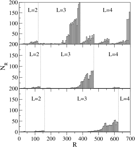
Figure 9: Number of communities in the recurrent sets vs. the resource saturation varying direct competition (upper panel, $\rho=0$; middle panel $=0.3$; lower panel, $\rho=0.7$). Observe the decrease in $N_{\mathcal{R}}$ as competition increases, and the increase of the values of $R$ at which a new level arises.

3.3 Dependence on the parameters

We have already mentioned that the model results are not qualitatively influenced by variations of its parameters. For example, we have studied the model dependence with respect to direct competition (Figure 9). In the absence of interspecific competition ($\rho=0$) levels are filled up more easily, so the number of communities in the recurrent set increases with respect to the results reported so far. The effect of increasing direct competition is to reduce the number of ecosystems in these sets, and to increase the resistance to the appearance of a new level in the end state for the same values of resource saturation. Thus, the global behavior of the number of communities as a function of $R$ turns out to be similar, up to scale factors, to that obtained in Capitán et al. (2009), Figure 3.

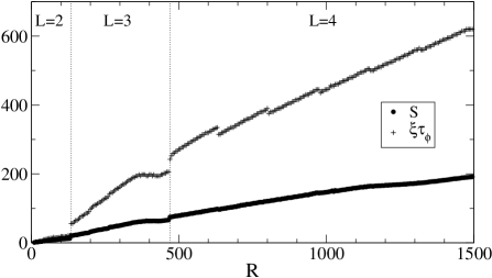
(a)     (b)

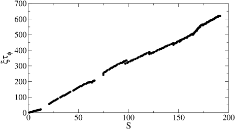
Figure 10: (a) Mean absorption time $\tau_{\varnothing}$ (in number of invasions) starting from the empty community $\varnothing$, and mean number of species $S$ as a function of the resource saturation $R$, showing a roughly linear growth for both of them. (b) Mean absorption time $\tau_{\varnothing}$ vs. $S$.

The particular case $\rho=1$ (interspecific competition equal to intraspecific competition) is qualitatively different. Fixing $\rho=1$ transforms the community into a trophic chain. All species can be grouped into a single one with population $N^{\ell}=s_{\ell}n^{\ell}$ [i.e. the Lotka-Volterra equations of this system (Capitán and Cuesta, 2010) are closed in the variables $N^{\ell}$]. But the implications of this assumption are stronger. Even if the distinction between species becomes meaningless, one can formally keep the identities and treat them as different. But then it is easy to show that any invasion attempted at a level already occupied by at least one species will be unsuccessful because the population of the invader ends up below $n_{c}$. In fact, according to Eq. (12) of Capitán and Cuesta (2010), the initial per capita growth rate of an invader at level $\ell$ is $-n_{c}$ and the equations for level ${\ell}$ and for the invader coincide. Hence $\dot{N^{\ell}}/N^{\ell}=\dot{n}/n$, $n$ being the abundance of the invader. This asymptotically yields

$$\bar{p}=\frac{n_{c}}{N^{\ell}(0)}\bar{P}^{\ell}$$ (3)

since $n(0)=n_{c}$ ($\bar{p}$ and $\bar{P}^{\ell}$ are the invader and the total $\ell$-level densities at equilibrium after the invasion, respectively). Now, the linear system (13) in Capitán and Cuesta (2010) for the interior equilibrium point before the invasion is exactly the same after the invasion replacing $N^{\ell}(0)$ by $\bar{p}+\bar{P}^{\ell}$. This fact, together with (3), yields $p=n_{c}N^{\ell}(0)/[n_{c}+N^{\ell}(0)]<n_{c}$. Since the population of the invader initially decreases, according to our extinction procedure (Capitán and Cuesta, 2010) the invader goes extinct.

Thus the assembly graph $\mathcal{G}$ becomes trivial. Using the notation $\{s_{\ell}\}_{\ell=1}^{L}$ for each community, $\mathcal{G}$ is simply

$$\varnothing\rightarrow\{1,0,\dots,0\}\rightarrow\{1,1,\dots,0\}\rightarrow\dots\rightarrow\{1,1,\dots,1\}.$$ (4)

This never happens if $\rho\neq 1$. Things are thus very different when this fully symmetric scenario is assumed.

It can be shown that in this fully symmetric scenario the competitive exclusion principle applies. This principle states that there can not coexist more populations than different resources (or ecological niches) in the long term if these populations depend linearly on the resources (Hofbauer and Sigmund, 1998). We can put this statement in mathematical terms. For the sake of simplicity, let us assume that there is a single trophic level with $S$ species predating on the resource (at rates $\gamma_{+i}$, $i=1,\dots,S$) and let us set a non-uniform direct competition $\rho_{ij}$ between pairs of species in that level. Let $n_{i}$ be the population density if species $i$, $a_{i}$ its death rate in the absence of consumption and $n_{0}$ the amount of resource. The Lotka-Volterra equations for this system are

$$\frac{\dot{n}_{i}}{n_{i}}=-a_{i}+\gamma_{+i}n_{0}-\sum_{j=1}^{S}\rho_{ij}n_{j}.$$ (5)

If the competition matrix is singular, we can find a non-trivial solution $(c_{1},\dots,c_{S})$ for the linear system $\sum_{i}c_{i}\rho_{ij}=0$, $j=1,\dots,S$ (note that, in particular, the fully symmetric scenario $\rho=1$ renders the competition matrix singular). Hence

$$\sum_{i=1}^{S}c_{i}(\log n_{i})\dot{\phantom{i}}=\sum_{i=1}^{S}c_{i}(\gamma_{+i}n_{0}-a_{i})\equiv-a$$ (6)

where we can assume that $a$ is positive (otherwise change the sign of the $c_{i}$). Integrating from 0 to $t$ we obtain

$$\prod_{i=1}^{S}n_{i}(t)^{c_{i}}=Ce^{-at}.$$ (7)

This means that one of the densities must vanish in the limit $t\rightarrow\infty$, which proves competitive exclusion.

There is a peculiarity of our model, though. If $\rho=1$ the population of the invader at equilibrium will not be zero because in our model all constants are uniform, so the equation to solve for $c_{i}$ is $\sum_{i}c_{i}=0$. This yields $a=0$ and spoils the argument. However, we have shown that, with our procedure of species extinction, the invader’s population ends up below $n_{c}$ hence not being viable. This restores competitive exclusion, albeit in a weaker sense. The result (4) is just a manifestation of this fact.

It is important to notice that, for a non-singular competition matrix, the competitive exclusion principle is not guaranteed to hold. In particular, if $\rho<1$ the intra- and interspecific competition will have different magnitude, and the matrix of elements $\rho_{ii}=1$ and $\rho_{ij}=\rho$ ($i\neq j$) will be non-singular. The argument above does not apply anymore and, as a matter of fact, by integrating the equations for population dynamics we actually obtain more than one species coexisting with a single resource in the system.

The interesting point brought about by the above discussion is that interspecific competition induces de facto a niche separation for the species of the same level —which are therefore competing for the same resources— that allows them to circumvent the competitive exclusion principle [for a more thorough discussion of this point see Bastolla et al. (2005a, b)].

3.4 Absorption times

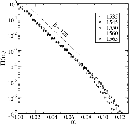
(a)          (b)

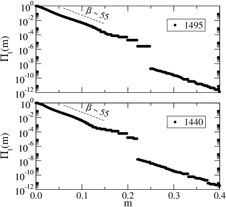
Figure 11: (a) Probability $\Pi(m)$ that an invasion causes the extinction of at least a fraction $m$ of the species of the invaded community, for several values of the resource saturation $R$. There is a characteristic magnitude $\beta^{-1}$ around 1%. In order to have enough statistics, we have chosen values of $R$ within the region where the number of communities in the recurrent set is above 1000 [see Figure 3 in Capitán et al. (2009)]. Thus we have better statistics to compute the histograms than for smaller $R$. (b) The same probability but for transient states, $\Pi_{\rm t}(m)$, for two values of $R$. The characteristic size of the avalanches here is about 2%.

So far we have discussed properties of the recurrent set of the Markov chain associated to the assembly process. But we have not discussed the possibility that the process may keep trapped for a long time in transient states. In order to ascertain this, we have calculated the mean absorption time from the empty community $\varnothing$ to the end state. This can be done given the structure that the transition matrix $P$ acquires after a permutation that reorders recurrent and transient states. We can thus write the matrix in a block form (Karlin and Taylor, 1975)

$$P=\left(\begin{array}[]{cc}U&0\\ W&V\end{array}\right),$$ (8)

where matrix $U$ contains the transition probabilities within the recurrent set, and $V$ contains transition probabilities between transient states. The average time from the transient state $i$, to reaching for the first time the recurrent set at state $j$ is the element $t_{ij}$ of matrix $T$, where

$$T=\sum_{n=1}^{\infty}nV^{n-1}W=(\mathbb{I}-V)^{-2}W,$$ (9)

$\mathbb{I}$ being the identity matrix. This expression counts as $n$ the absorption time when the process remains $n-1$ time steps within the transient subset and jumps to a recurrent state in the $n$-th step. The mean absorption time for a process starting from the transient state $i$ will thus be $\tau_{i}=\sum_{j\in\mathcal{R}}t_{ij}=(Tu)_{i}$, where $u=(1,\dots,1)^{T}$. Since $P$ is stochastic, $\sum_{j}(V_{ij}+W_{ij})=(Vu)_{i}+(Wu)_{i}=1$ for all $i\in\mathcal{G}-\mathcal{R}$, so $Wu=(\mathbb{I}-V)u$ or, equivalently, $(\mathbb{I}-V)^{-1}Wu=u$. Together with (9) this implies $(\mathbb{I}-V)\tau=u$, so solving this sparse linear system yields the absorption times for any transient state. Note that these times are proportional to $\xi^{-1}$, because of the form (1) of our transition matrix.

In Figure 10a we plot the mean absorption time $\tau_{\varnothing}$ to reach the recurrent set starting from the empty community, along with the mean number of species $S$, which measures the size of the system. Both of them grow almost linearly with $R$, hence $\tau_{\varnothing}$ is roughly linear with $S$ as well (see Figure 10b). Since the number of states in each chain grows as $e^{\kappa\sqrt{R}}$, the number of states of the Markov chain is very large compared to $\xi\tau_{\varnothing}$. Therefore the mean time to the end state is small compared to the system size.

This result should be taken with a grain of salt, because it strongly relies on our assignment of probabilities to transitions. This, in turn, assumes that there is always availability of invaders, which may not be true if invaders come from a finite pool. The lack of potential invaders when the community is almost “full” would decrease the probability of a new invasion and accordingly would increase the time that the process needs to reach the end state. What the result of Figure 10a is actually telling us is that the assembly graph is dominated by pathways in which most invasions are accepted.

3.5 Extinctions distribution

As we have previously described, the assembly process can be regarded as if the ecosystem self-organizes into a state resistant to invasions. Either for transient or recurrent states, the community is continuously undergoing avalanches of extinctions caused by new colonizations. Figure 11a shows a statistics of such avalanches in some recurrent sets. It represents the probability $\Pi(m)$ that an invasion causes an avalanche of magnitude greater than $m$ (understood as the fraction of species that go extinct), averaged over the stationary state. We can see in the figure that this probability shows an exponential decay, with a typical avalanche size $\beta^{-1}$ of about $1\%$ of the community, $\beta$ being the slope of the distributions in log-linear scale. Invasions never cause big perturbations in the community.

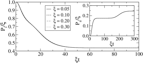
(a) (b)

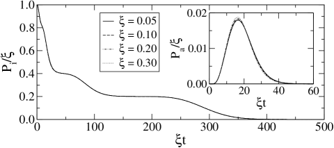
(c)

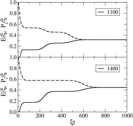
Figure 12: (a) Probability of invasion vs. mean number of invasions ($\xi t$) for $R=430$ (with a complex end state). Inset: probability of reconfiguration after invasion vs. mean number of invasions. (b) The same as (a) but for $R=540$ (the end state is a single community). (c) Probability of invasion (dashed lines) and average number of species loss (full lines) vs. mean number of invasions, for two values of $R$ with complex end states. At the time these two magnitudes coincide, a stationary state (the recurrent set) is reached.

We can calculate a similar distribution for the avalanches of extinctions in the transient states. Now we have to weight the magnitudes with the average fraction of visits to each transient state. Let us denote as $z_{ij}$ the average number of visits to state $j$ starting from state $i$. The matrix $Z=(z_{ij})$ is then given by

$$Z=\sum_{n=0}^{\infty}V^{n}=(\mathbb{I}-V)^{-1}.$$ (10)

Thus the number of visits to the transient $j$ starting from $\varnothing$ is $\zeta_{j}=(u_{\varnothing}Z)_{j}$, $u_{\varnothing}$ being the row vector $\delta_{i\varnothing}$ (with a number of entries equal to the number of transient states). We can calculate $\zeta$ by solving the linear system

$$\zeta(\mathbb{I}-V)=u_{\varnothing}.$$ (11)

The resulting probability $\Pi_{\rm t}(m)$ that an invasion causes the extinction of at least a fraction $m$ of the species of the invaded transient community is showed in Figure 11b. We also find an exponential behavior for the cumulative distribution, in this case with a mean characteristic fraction of species loss of 2% for transient avalanches. The species loss caused by invasions in the transient part of the graph is always small.

3.6 Time averages

Computing the time evolution of averages is very simple, given the transition matrix $P$ and some initial probability distribution (Karlin and Taylor, 1975) —which in our case is simply the vector $u_{\varnothing}$, since the assembly process starts from the empty community. We just need to calculate the power $P^{t}$ to obtain the transition probability matrix after $t$ time steps. Thus we can obtain the probability of rejecting the invader at discrete time $t$ as

$$P_{\rm r}(t)=\sum_{j}P_{jj}(P^{t})_{j\varnothing},$$ (12)

and that of accepting the invader as

$$P_{\rm i}(t)=\sum_{j}\bigg{(}\sum_{|k-j|=1}P_{jk}\bigg{)}(P^{t})_{j\varnothing},$$ (13)

where the inner sum runs over transitions from $j$ in which the invader is accepted. Obviously, the probability that the community undergoes a reconfiguration because of the invasion is obtained as $P_{\rm a}(t)=1-P_{\rm r}(t)-P_{\rm i}(t)$. Figures 12a and 12b represent the dependence in time of the probabilities $P_{\rm i}$ and $P_{\rm a}$ in two cases: one with a a complex end state (a), and another with a single community as end state (b). Notice that all curves collapse, for small $\xi$, when divided by $\xi$ and plotted against $\xi t$ (mean number of invasions).

In Figure 12c we show the probability of invasion $P_{\rm i}(t)$ and the average species loss defined as

$$E(t)=\sum_{j}\bigg{(}\sideset{}{{}^{\prime}}{\sum}_{k}(\Delta S)_{jk}P_{jk}\bigg{)}(P^{t})_{j\varnothing},$$ (14)

where $(\Delta S)_{ij}$ is the species loss in the transition from $j$ to $k$ and the prime denotes that we ignore in the sum transitions in which the invader is accepted. When these two magnitudes are equal there is an equilibrium between the average frequency of invasions and the average number of species loss. This is a fingerprint of the reaching of the stationary state. As expected, this time is comparable to the absorption time shown in Figure 10a.

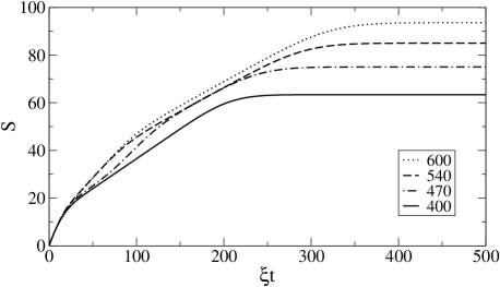
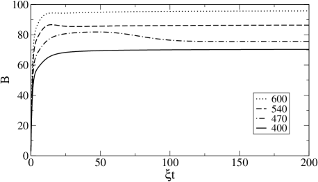
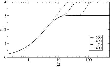
(a)     (b) (c)          (d)

Figure 13: Species richness (a) and total population (b) vs. mean number of invasions ($\xi t$), for several values of the resource saturation $R$. At $R=470$ (showed with dash dotted lines) the ecosystem crosses over from $3$ levels to $4$ levels (this crossover corresponds to the non-monotonic behavior of the total population). (c) Mean number of levels vs. mean number of invasions. At the onset of the fourth level, the ecosystem stays some time trapped in three-level communities. (d) Typical variation of the average return time with $\xi t$.

Another important magnitude is biodiversity. Figure 13a represents the evolution of the average number of species for several values of $R$. In all cases, this average number grows monotonically until reaching the stationary state, so biodiversity and resistance to invasion are positively correlated, in agreement with previous assembly models (Law and Morton, 1996; Morton and Law, 1997).

Figure 13b represents the evolution of the total population density $B$ of each community. If we assume, for the sake of simplicity, the same weight per individual for all species in our model communities, then $B$ can be regarded as the total biomass in the community. Although there is a clear trend for biomass to increase, it is not always at its optimum in the stationary state. This is very clear in the figure for $R=470$, a value at the onset of the appearance of the fourth trophic level. This agrees with the analysis performed by Virgo et al. (2006) on their assembly model.

We have also studied the time dependence of the average number of trophic levels during the assembly, which is shown in Figure 13c. At $R=470$ the process stays a certain time trapped in three-level communities until the fourth level is finally accepted. This effect becomes lower upon increasing $R$, until there is no trapping and the fourth level is reached straight away.

Figure 13d shows a typical time evolution of the average return time along the assembly until reaching the stationary state. Communities are less resilient (have larger return time to equilibrium) as time increases. Thus, there is a trade-off between robustness (resistance against invasions) of the ecosystem and dynamic stability which is resolved by sacrificing the latter in favor of the former.

4 Discussion

In this work we have provided a full account of results of the model introduced in Capitán et al. (2009). The results presented here have been obtained from a direct analysis of the Markov chain describing the assembly process. Among the novel results here presented are the dependence of many biological observables on the amount of available resource (implemented through parameter $R$), the average times that the process needs to reach the recurrent set, the statistics of avalanches in both transient and recurrent states, and the time evolution of any observable.

Our model might be considered as a benchmark of the assembly process that builds up ecological communities. As such, we do not aim at providing a realistic description of an ecosystem but at capturing, in a very simplified model, the essential mechanisms that do occur in the construction of real ecosystems. The model rests on some oversimplistic features: communities are strictly organized in levels, predation occurs only between contiguous levels, species of a given level are trophically equivalent, model parameters are chosen uniformly and the population dynamics is ruled by simple Lotka-Volterra equations. In spite of this, our model exhibits the same behavior as all other assembly models reported in the literature. This indicates that this behavior is very robust, and probably shared by real systems and simple models alike.

Thanks to these oversimplifications the model provides important advantages on previous assembly models. The main one is that we can trace all pathways of the assembly process. This allows us to compute exactly all the observables of a community and to characterize in a very precise manner the stationary state of the ecosystem. Our model also has a species pool, as standard assembly models, but because we allow for an arbitrary number of trophically equivalent species, the pool is infinite and the model does not suffer from the problem of exhaustion of good invaders that may trap the community in a transient state (Case, 1991; Levine and D’Antonio, 1999). This has permitted us to build communities with hundreds of species and explore the influence of different elements on the behavior of the assembly process.

Therefore, we are not limited, as in standard assembly models, to compute averages over a set of realizations of the process. As we pointed out in Capitán et al. (2009), the number of shortest pathways leading from $\varnothing$ to the recurrent set can be enormous. For instance, for $R=300$ (a case with an absorbing community of three trophic levels and 50 species), there are $\sim 10^{10}$ different minimum-length pathways. This number is far from anything a simulation can come close to.

There is, of course, a concern about having trophically equivalent —hence indistinguishable— species. The grouping of trophically equivalent species is a common practice in studying food webs, so it is tempting to do so in this model. If we do it, the model becomes equivalent to a chain, for which Lotka-Volterra dynamics is well characterized (Hofbauer and Sigmund, 1998), and the invasion process seems to become trivial. This is not true, though: if $\rho\neq 1$, i.e. if intra- and interspecific competition are different in magnitude, intraspecific competition in the equivalent chain explicitly depends on $s_{\ell}$, so invasions modify the parameters of the chain and the invasion process becomes non trivial. Thus, it is because of the direct interspecific competition $\rho<1$ that this equivalence breaks down and the model departs from triviality. We have explicitly shown that choosing $\rho=1$ brings about the competitive exclusion principle, and indeed the model turns into a chain. But for any $\rho<1$ this does not longer hold. Interspecific competition is thus an effective way of creating new niches.

Let us now summarize the main conclusions we can extract from the present analysis of the model.

As our model ecosystems evolve we observe three trends: biodiversity increases, resistance to invasion increases and all species decrease their populations. In the steady state biodiversity is at its maximum, all populations are close to the extinction level and either invasions are rejected or they produce transitions between a set of communities with a very similar structure. All three features are related. The increase in biodiversity is unavoidable because of the constant flux of colonizers; however, as the number of species increases, their populations necessarily decrease because all share the same resource. The invasion process guarantees that this is done in the most efficient way, because inefficient invasions cause extinctions in the community and force a more equilibrated rearrangement of the populations. This, in turn, justifies the increasing resistance to new invasions. At the end, all populations are so close to extinction that either no new invasions are possible, or they just cause small rearrangements that leave the community in a similar state.

Final communities have typically three or four trophic levels —only ecosystems with more than $200$ species generate five trophic levels. On the other hand, the number of species in each level has a pyramidal structure. Both features are in qualitative agreement with what is observed in real ecosystems (Cohen et al., 1990) and we have discussed at length the properties of the population dynamics equations that explain these features in Capitán and Cuesta (2010).

As already advanced in Capitán et al. (2009) the end state is always unique, and this is consistent with previous assembly models (Morton and Law, 1997). However, there is a caveat that should be made on this point related to the indistinguishability of species within the same trophic level: the end state is unique as long as we consider only the number of species at each level. Whether two communities with the same numbers have the same or different species is meaningless for this model, so the conclusion is not definitive. In fact, some relatively recent experiments on aquatic microbial communities establish that productivity-biodiversity relationships depend on the history of assembly (Fukami and Morin, 2003), and it is our guess that the independence on history resulting from this model might be an artifact of the indistinguishability of species. Refined versions of this model may clarify this issue.

As for the robustness of the above results, we have tried other values of the direct competition parameter, namely $\rho=0$ and $\rho=0.7$, to test its influence. No qualitative difference with the behavior reported here is found. Nonetheless, there are three quantitative effects that we have observed as $\rho$ increases: resistance to invasion increases, appearance of new trophic levels is hindered and the number of communities in complex end states decreases. Varying $\gamma_{-}$ has similar effects; in fact, the product $\gamma_{+}\gamma_{-}=0.1\gamma_{-}^{2}$ provides a quantitative estimate of indirect competition.

It can be argued that parameters should depend on the trophic level rather than being uniform for all species. It is very easy to show that this does not change the dynamic stability patterns because in that case one can also construct a Lyapunov function [see Capitán and Cuesta (2010)]. We have not attempted any test in this respect, but it is hard to believe that such a variant of the model will produce any qualitative difference. The assembly graphs will be similar to the ones found for the present model. Something more can be said about the invasion rate. We have presently assumed that the invasion probability is the same for all trophic levels, but notice that the assembly graph is utterly independent on this choice, so certainly choosing a different invasion probability will change the numerical value of the nonzero entries of the transition matrix $P$, but only them. The graph, as well as the structure of transient and recurrent states of a finite Markov chain, only depends on which elements of $P$ are zero (Karlin and Taylor, 1975), so not just the graph but the set of communities in the end state will be exactly the same as those reported here (the probability distribution in the steady state will, of course, be different).

Perhaps the most important limitation of this model is the choice of the Lotka-Volterra equations. The choice of population dynamics has been reported to have a strong influence in the final shape of ecological communities (Drossel et al., 2004; Lewis and Law, 2007). Introducing non-linear equations leads to more complex stability patterns than simply rest points. How to account for them is not yet clear to us, but neither is whether this will really affect the qualitative behavior of the assembly process. Thus, this remains an important open question that deserves further analysis.

There are further open questions such as the application of this model to metacommunities. The resulting ecosystems can be readily altered when migration takes place among spatially distributed patches. With a simple model like ours, it might be possible to build up an assembly graph between different communities in different patches. The interplay between communities in different patches could lead to an outcome different from the one we obtain with a single patch. On the other hand, a simple model like this can provide us with basic understanding of complex processes such as, for instance, the rebuilding of a natural community after its degradation. Very little is known about the processes that helps to reconstruct damaged communities, and a simple framework like ours could provide some hints about how to tackle this problem from a theoretical point of view.

The final take-home message from this work is this: we should not be afraid of oversimplifications in complex systems. Complexity normally arises as a consequence of a collective behavior of many entities, not as a result of the complexity of interactions. The key point is whether we are retaining the basic ingredients yielding the desired output. We have shown that there is no qualitative difference between the results of this oversimplified model and previous, more sophisticated assembly models. And there is a lot to gain from the wider view that this model provides of the process and the much higher control we have on the parameters. Many questions that are hard (or even impossible) to answer in previous model have a clear-cut answer here. And even if they may be too simplistic, they can still guide our intuition when dealing with real ecosystems.

5 Acknowledgements

This work is funded by projects MOSAICO, from Ministerio de Educación y Ciencia (Spain) and MODELICO-CM, from Comunidad Autónoma de Madrid (Spain). J. A. Capitán also acknowledges financial support through a contract from Consejería de Educación of Comunidad de Madrid and Fondo Social Europeo. J. B. is funded by the European Heads of Research Councils, the European Science Foundation, and the EC Sixth Framework Programme through a EURYI (European Young Investigator) Award.

References

- Bastolla et al. (2005a) Bastolla, U., Lässig, M., Manrubia, S.C., Valleriani, A., 2005a. Biodiversity in model ecosystems, i: coexistence conditions for competing species. J. Theor. Biol. 235, 521–530.
- Bastolla et al. (2005b) Bastolla, U., Lässig, M., Manrubia, S.C., Valleriani, A., 2005b. Biodiversity in model ecosystems, ii: species assembly and food web structure. J. Theor. Biol. 235, 531–539.
- Capitán and Cuesta (2010) Capitán, J.A., Cuesta, J.A., 2010. Species assembly in model ecosystems, i: Analysis of the population model and the invasion dynamics .
- Capitán et al. (2009) Capitán, J.A., Cuesta, J.A., Bascompte, J., 2009. Statistical mechanics of ecosystem assembly. Physical Review Letters 103, 168101–4.
- Case (1990) Case, T.J., 1990. Invasion resistance arises in strongly interacting species-rich model competition communities. Proc. Natl. Acad. Sci. USA 87, 9610–9614.
- Case (1991) Case, T.J., 1991. Invasion resistance, species build-up and community collapse in metapopulation models with interspecies competition. Biol. J. Linn. Soc. 42, 239–266.
- Cohen et al. (1990) Cohen, J.E., Briand, F., Newman, C.M., 1990. Community food webs. Springer-Verlag, Berlin.
- Drake (1990) Drake, J.A., 1990. The mechanics of community assembly and succession. J. Theor. Biol. 147, 213–233.
- Drossel et al. (2004) Drossel, B., McKane, A.J., Quince, C., 2004. The impact of nonlinear functional responses on the long-term evolution of food-web structure. J. Theor. Biol. 229, 539–548.
- Dunne (2006) Dunne, J.A., 2006. The network structure of food webs, in: Pascual, M., Dunne, J.A. (Eds.), Ecological Networks. Oxford University Press, Oxford, pp. 27–86.
- Fukami and Morin (2003) Fukami, T., Morin, P.J., 2003. Productivity-biodiversity relationships depend on the history of community assembly. Science 424, 423–426.
- Hofbauer and Sigmund (1998) Hofbauer, J., Sigmund, K., 1998. Evolutionary games and population dynamics. Cambridge University Press, Cambridge.
- Karlin and Taylor (1975) Karlin, S., Taylor, H.M., 1975. A first course in stochastic processes. Academic Press, New York.
- Knuth (1997) Knuth, D., 1997. The art of computer programming vol. 1. Fundamental algorithms. Addison-Wesley, Reading, Massachusetts.
- Law and Morton (1993) Law, R., Morton, R.D., 1993. Alternative permanent states of ecological communities. Ecology 74, 1347–1361.
- Law and Morton (1996) Law, R., Morton, R.D., 1996. Permanence and the assembly of ecological communities. Ecology 77, 762–775.
- Levine and D’Antonio (1999) Levine, J.M., D’Antonio, C.M., 1999. Elton revisited: a review of evidence linking diversity and invasibility. Oikos 87, 15–26.
- Lewis and Law (2007) Lewis, H.M., Law, R., 2007. Effects of dynamics on ecological networks. J. Theor. Biol. 247, 64–76.
- McCann (2000) McCann, K.S., 2000. The diversity-stability debate. Nature 405, 228–233.
- Morton and Law (1997) Morton, R.D., Law, R., 1997. Regional species pools and the assembly of local ecological communities. J. Theor. Biol. 187, 321–331.
- Morton et al. (1996) Morton, R.D., Law, R., Pimm, S.L., Drake, J.A., 1996. On models for assembling ecological communities. Oikos 75, 493–499.
- Pimm (1991) Pimm, S.L., 1991. The balance of nature: Ecological issues in the conservation of species and communities. University of Chicago Press, Chicago.
- Pimm and Lawton (1977) Pimm, S.L., Lawton, J.H., 1977. The number of trophic levels in ecological communities. Nature 268, 329–331.
- Post and Pimm (1983) Post, W.M., Pimm, S.L., 1983. Community assembly and food web stability. Math. Biosc. 64, 169–192.
- Roughgarden (1974) Roughgarden, J., 1974. Scpecies packing and the competition function with illustrations form coral reef fish. Theor. Population Biol. 5, 163–186.
- Turelli (1981) Turelli, M., 1981. Niche overlap and invasion of competitors in random evironments i: models without demographic stichaticity. Theor. Population Biol. 20, 1–56.
- Virgo et al. (2006) Virgo, N., Law, R., Emmerson, M., 2006. Sequentially assembled food webs and extremum principles in ecosystem ecology. J. Anim. Ecol. 75, 377–386.
- Warren et al. (2003) Warren, P.H., Law, R., Weatherby, A.J., 2003. Mapping the assembly of protist communities in microcosms. Ecology 84, 1001–1011.
- Xie and Beerel (1998) Xie, A., Beerel, P.A., 1998. Efficient state classification of finite-state markov chains. IEEE T. Comput. Aid. D. 17, 1334–1339.