Magnetostatics of synthetic ferrimagnet elements

Abstract

We calculate the magnetostatic energy of synthetic ferrimagnet (SyF) elements, consisting of two thin ferromagnetic layers coupled antiferromagnetically, e.g. through RKKY coupling. Uniform magnetization is assumed in each layer. Exact formulas as well as approximate yet accurate ones are provided. These may be used to evaluate various quantities of SyF such as shape-induced coercivity and thermal stability, like demagnetizing coefficients are used in single elements.

Synthetic antiferromagnets (SAF, resp. ferrimagnets, SyF)[1, 2] consist of two thin ferromagnetic films of moments of same (resp. different) magnitude, strongly coupled antiferromagnetically thanks to the RKKY interaction through an ultrathin spacer layer, typically Ru $0.6-0.9\,\mathrm{nm}$ thick[3]. Hereon we consider only the case of in-plane magnetized layers. SyFs are widely used to provide spin-polarized layers displaying an overall weak moment. One benefit is to minimize cross-talk of neighboring (e.g. memory bits) or stacked (e.g. in a spin-valve) elements through stray-field coupling[1, 2], such as in Magnetic Random Access Memory (MRAM)[4]. SyFs are also used to decrease the Zeeman coupling with external fields, e.g. to increase coercivity in reference layers[5], decrease effects of the Oersted field in magneto-resistive or spin-torque oscillator pillars, or more recently boost the current-induced domain-wall propagation speed in nanostripes[6, 7].

In practice SyFs are used as elements of finite lateral size. It has been shown[8] and it is widely used [9, 10] that for flat and magnetically soft nanomagnets of lateral size smaller than a few hundreds of nanometers, the macrospin approximation (uniform magnetization) is largely correct. In this framework the coercive field equals the anisotropy field $2K/\mu_{\mathrm{0}}M_{\mathrm{s}}$ and the energy barrier $KV$ ($V$ is the volume of the dot) preventing spontaneous magnetization reversal equals the magnitude of anisotropy of the total magnetic energy $\mathcal{E}$, to which all the physics therefore boils down. Elongated dots are often used to induce or contribute to an easy axis of magnetization and an energy barrier $\Delta\mathcal{E}$, based on dipolar energy. Dipolar energy is a quadratic form and thus it is fully determined by its value along the two main in-plane axes. For single elements $\Delta\mathcal{E}_{\mathrm{d}}=K_{\mathrm{d}}V\Delta N$ with $\Delta N$ the difference between the two in-plane demagnetizing coefficients, and $K_{\mathrm{d}}=(1/2)\mu_{\mathrm{0}}M_{\mathrm{s}}^{2}$.

Analytical formulas have been known for a long time to evaluate the mutual energy of an arbitrary set of prisms[11]. However while simple expressions for $N$ and thus $\Delta\mathcal{E}_{\mathrm{d}}$ have been described, displayed and discussed for single-layer flat elements[11, 12], the analytical expressions and the evaluation of $\mathcal{E}_{\mathrm{d}}$ in SyFs have not been discussed in detail so far. Instead the studies requiring estimation of the dipolar energy in SyF, mainly pertaining to MRAM cells[9, 10, 13], have in the best case made use of an effective so-called attenuation coefficient with respect to self-energy[10], which requires a numerical evaluation[13]. The meaning and scaling laws of this attenuation coefficient have never been discussed in detail, hiding the physics at play. As thermal stability, coercivity and toggle switching fields[9, 10, 14] depend crucially on the interlayer magnetostatic coupling, it is desirable to have a simple yet accurate analytical expression for interlayer dipolar fields. In this manuscript we report exact analytical expressions for the magnetostatics of SyFs uniformly-magnetized in each sub-layer. From the numerical evaluation we discuss the physics at play, while from the analytical formulas we propose an approximate yet accurate scaling law for their straightforward table-top evaluation.

Figure 1: Geometry and notations of a prismatic SyF element comprising two ferromagnetic layers $\mathrm{F}_{1}$ and $\mathrm{F}_{2}$.

We first consider SyF prisms and name F1 and F2 the two ferromagnetic layers (Figure 1), with magnetization aligned along $z$. This covers the case of both finite-size prisms as well as infinitely-long stripes with a rectangular cross-section. We apply formulas expressing the interaction between two parallel charged surfaces[11], and adopt the convenient notation of $F_{ijk}$ functions, the $i$, $j$ and $k$-fold indefinite integrals along $x$, $y$ and $z$ of the Green’s function $F_{000}=1/r$[15]. The only such function needed here is

$$F_{220}=\frac{1}{2}[x(v-w)L_{x}+y(u-w)L_{y}]-xyP_{z}+\frac{1}{6}r(3w-r^{2})$$ (1)

with $u=x^{2}$, $v=y^{2}$, $w=z^{2}$, $r=\sqrt{u+v+w}$, $L_{x}=(1/2)\ln[(r+x)/(r-x)]$ etc, $P_{x}=x\arctan(yz/xr)$ etc, and $L_{x}=0$ and $P_{x}=0$ for $x=0$ etc.

The integrated magnetostatic energy of a single prismatic element of thickness $t$ is:

$$\mathcal{E}_{\mathrm{d}}=\frac{2K_{\mathrm{d}}}{\pi}\sum_{\delta_{a},\delta_{t},\delta_{c}\in\{0,1\}}(-1)^{\delta_{a}+\delta_{t}+\delta_{c}}F_{220}(a\delta_{a},t\delta_{t},c\delta_{c})$$ (2)

which normalized to $K_{\mathrm{d}}$ yields the demagnetizing coefficient $N_{z}$. It can be verified that Eq. (2) coincides with the explicit formula already known[12]. The magnetostatic energy of a prismatic SyF element may be calculated using the same formalism , may be written as:

$$\mathcal{E}_{\mathrm{d}} = K_{\mathrm{d,1}}N_{z}(a,t_{1},c)V_{1}+K_{\mathrm{d,2}}N_{z}(a,t_{2},c)V_{2}$$ (3)

$$+2\sqrt{K_{\mathrm{d,1}}K_{\mathrm{d,2}}}N_{\mathrm{m}}(a,t_{1},s,t_{2},c)\sqrt{V_{1}V_{2}}$$

with $N_{\mathrm{m}}(a,t_{1},s,t_{2},c)=\frac{1}{\pi a\sqrt{t_{1}t_{2}}c}\sum_{\delta_{1},\delta_{2},\delta_{a},\delta_{c}\in\{0,1\}}(-1)^{\delta_{1}+\delta_{2}+\delta_{a}+\delta_{c}}\times F_{220}(a\delta_{a},s+t_{1}\delta_{1}+t_{2}\delta_{2},c\delta_{c})$ is a mutual magnetostatic coefficient with a negative value, and $V_{i}=at_{i}c$ (resp. $K_{\mathrm{d,i}}$) is the volume (resp. dipolar constant) of each single prism $i$. This equation of dipolar energy is a quadratic form of $M_{1}$ and $M_{2}$, generalizing the definition of demagnetizing coefficients.

Figure 2(a) shows $\mathcal{E}_{\mathrm{d}}$ upon building a SyF via the progressive thickness increase of F2 above F1, considering or not the interaction between the two layers. In the latter case the energy increase nearly scales with $t_{2}^{2}$, which is understandable because it is a self-energy (in $\mathrm{F}_{2}$ alone). In the coupled case (a SyF) $\mathcal{E}_{\mathrm{d}}$ retains like for the uncoupled case an overall close-to-parabolic convex shape as can be verified with fitting, however with an initial negative slope. This can be understood as for low $t_{2}$ the extra edge charges induced by an infinitesimal increase $\delta t_{2}$ mainly feel the stabilizing stray field arising from F1, while for large $t_{2}$ they feel more the nearby charges induced by F2 itself. Notice that, contrary to what could be a first guess, the minimum of $\mathcal{E}_{\mathrm{d}}(t_{2})$ occurs before the compensation of moment ($t_{1}=t_{2}$). This stems from the same argument as above, which is that magnetic charges at an edge of F2 are closer to another than to the charges on the nearby edge of F1, thus for an identical amount $\delta t_{2}$ contribute more to $\mathcal{E}_{\mathrm{d}}$.

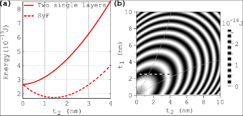
Figure 2: Magnetostatic energy of a SyF with $c=2a=100\,\mathrm{nm}$, $M_{1,2}=10^{6}\,\mathrm{A/m}$, $s=0.7\,\mathrm{nm}$. (a) Sum of the energies of two prisms without mutual interaction, and when embedded in the SyF geometry. $t_{1}$ is kept constant at $2.5\,\mathrm{nm}$, while $t_{2}$ is varied. (b) Energy of the general SyF. The curved lines are those of minimum energy for either constant $t_{1}$ or $t_{2}$. The thick horizontal dotted line highlights the path for the SyF curve shown in (a).

Figure 2(b) shows the full plot of $\mathcal{E}_{\mathrm{d}}(t_{1},t_{2})$ for $s=0.7\,\mathrm{nm}$. The above arguments appear general. From this figure let us outline three take-away messages. 1. For a given $t_{1}$ the minimum of $\mathcal{E}_{\mathrm{d}}$ of a SyF is found for $t_{2}\gtrsim t_{1}/2$. 2. At this minimum $\mathcal{E}_{\mathrm{d}}$ is reduced by only $\approx 20\mathrm{-}30\,\mathrm{\%}$ with respect to a single-layer element of thickness $t_{1}$ considered alone. 3. $\mathcal{E}_{\mathrm{d}}$ roughly regains the value of the single layer at the moment compensation point ($t_{1}=t_{2}$).

This sheds light on results previously noticed empirically, however whose origin and generality had not been highlighted. Wiese et al. reported that the effective dipolar field anisotropy of a SyF basically scales with the inverse net moment[16], i.e. like the inverse strength of Zeeman energy. This suggests that $\Delta\mathcal{E}_{\mathrm{d}}$ is essentially independent of the imbalance of moment, which goes against the widespread belief that magnetostatic energy nearly vanishes upon moment compensation. Our results clarify and quantify this: the dipolar energy does not differ more than 20-30 % from that of a single layer for $t_{2}\lesssim t_{1}$ (Figure 2a, dotted line). Saito et al. also reported that the thermal stability of $\mathrm{Co}_{90}\mathrm{Fe}_{10}[3]\leavevmode\nobreak\ /\mathrm{Ru}[0.95]\leavevmode\nobreak\ /\mathrm{Co}_{90}\mathrm{Fe}_{10}[5]$ is similar to that of $\mathrm{Co}_{90}\mathrm{Fe}_{10}[3]$. As explained in the introduction, we recall that thermal stability is determined by the energy barrier along the hard axis direction, with respect to the easy axis direction. In the case of anisotropy arising from dipolar energy and an elongated shape of the element, this barrier can be evaluated straightforwardly by calculating once $\mathcal{E}_{\mathrm{d}}$ along the short edge of the dot, and second along the long edge of the dot. Doing this we explain the findings of Saito et al.., whereas a reduction of $50\,\mathrm{\%}$ would be expected on the basis of compensated moments (the numbers in brackets are thicknesses in nanometers). Our calculations may also be applicable to the cross-over of vortex versus single domain in flat disks[17] or vortex versus transverse domain walls in stripes[18], whose scaling law $t\times a=\mathrm{Cte}$ may be derived qualitatively by equaling the energy of a vortex $\sim t$ and that of a single-domain $\sim a^{2}t(t/a)$ (here $V=a^{2}t$ is the volume, and $t/a$ the demagnetizing coefficient). Interestingly Tezuka et al. noticed that there is an optimum ferromagnetic film thickness at which SyAF can obtain a single-domain structure. This minimum (related to a minimum of demagnetization energy) is found for an imbalanced thickness in good quantitative agreement with Figure 2b.

With a view to promote the use of accurate magnetostatics for SyF while eliminating the need for numerical evaluation, we derived approximate yet highly accurate expressions for $\mathcal{E}_{\mathrm{d}}$. Figure 3a shows that to a very good approximation, $\mathcal{E}_{\mathrm{d}}$ is proportional to the width of the element (along $x$) and is independent of its length (along $z$). This is already accurate for a single-layer ($t_{2}=0$), and is very accurate close to the compensation $t_{1}=t_{2}$ because edges then behave as lines of dipoles, whose stray field quickly decays with distance ($\sim 1/r^{2}$). Thus $\mathcal{E}_{\mathrm{d}}$ boils down to a single line integral along its edge:

$$\mathcal{E}_{\mathrm{d}} = E_{\lambda}\oint(\mathbf{m}.\mathbf{n})^{2}\mathrm{d}s$$ (4)

$$= E_{\lambda}\oint\frac{|\mathrm{d}x|}{\sqrt{1+(\partial_{x}f)^{2}}}$$ (5)

$$= E_{\lambda}\int_{0}^{2\pi}\frac{(r\sin\theta-\partial_{\theta}r\cos\theta)^{2}}{\sqrt{(\partial_{\theta}r)^{2}+r^{2}}}\mathrm{d}\theta$$ (6)

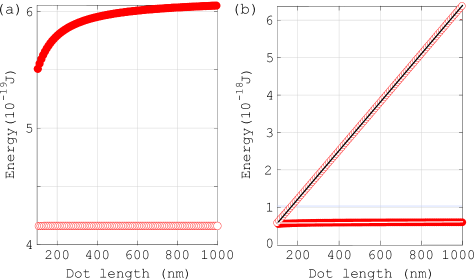
Figure 3: (a) Energy of a single layer (full symbols) and SyF (open symbols) as a function of dot length, i.e. along $z$, while $a=100\,\mathrm{nm}$. (b) Energy of a single layer as a function of width (along $x$, open symbols), and length (along $z$, full symbols, same curve as in a), while the other in-plane dimension is kept constant at $100\,\mathrm{nm}$. The lines are linear fits. For both plots the parameters are: $M_{i}=10^{6}\,\mathrm{A/m}$, $t_{1}=t_{2}=2.5\,\mathrm{nm}$, $s=0.7\,\mathrm{nm}$.

Eq. (4) is the general expression, expressed in the following two lines in cartesian and polar coordinates (Figure 4a). $E_{\lambda}$ is the density of magnetostatic energy per unit length of edge, a concept once discussed in the case of single layers[19]. Equations (4-6) apply to an arbitrary shape of perimeter (not simply rectangles for prisms) by considering the in-plane angle $\varphi$ between magnetization and the normal to the edge. It can be verified that for a SAF we have, with an accuracy better than $10\,\mathrm{\%}$ for geometrical parameters relevant for practical cases, i.e. $t_{1,2}$ in the range of $2-10\,\mathrm{nm}$ and $sintherangeof0.5-1\,\mathrm{nm}$:

$$E_{\lambda}\approx(1/2)K_{\mathrm{d}}t^{2}$$ (7)

The meaning of Eq. (7) is straightforward: due to the short range of interaction between dipolar lines, the density of dipolar energy is non-zero only in the vicinity of the edges, with a lateral range $t$. Thus a volume $t^{2}$ is concerned with a line density of energy of the order of $K_{\mathrm{d}}$. Expressions for non-compensated cases (including single elements) may also be evaluated. This provides us with analytical expressions for the magnetostatics of SyFs for the most usual shapes (Figure 4b).

A scaling law sometimes used as a first guess is based on the point dipole approximation. In this framework the energy gained by coupling $\mathrm{F}1$ and $\mathrm{F}2$ would roughly scale with $K_{\mathrm{d}}a^{4}/t$, resulting from two point moments $M_{\mathrm{s}}a^{2}t$ interacting like $1/t^{3}$ (for $s\ll t$, and assuming lateral dimensions of the order of $a$). The scaling arising from our exact calculation is $aE_{\lambda}\sim K_{\mathrm{d}}at^{2}$ (Eq. (7) and Figure 4a). The point dipole approximation is thus clearly incorrect with an extra scaling $(a/t)^{3}$ (see Figure 4a) which largely overestimates the dipolar coupling. This is a general argument for any flat element, where dipolar fields are short-ranged[20] and thus the point-dipole approximation is clearly incorrect.

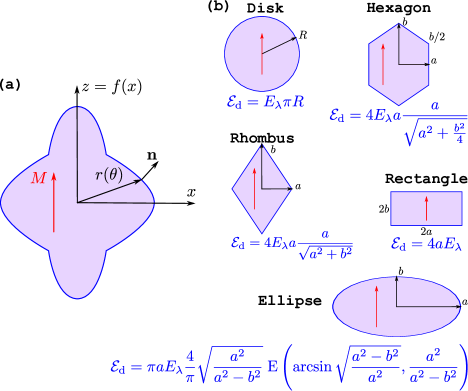
Figure 4: (a) notations for the calculation of edge energy (b) integrated magnetostatic energy for various shapes. $\mathrm{E}$ is the elliptical integral of the second kind. See text for the definition of $E_{\lambda}$.

To conclude we derived exact formulas for the magnetostatics of prism SyF, and simple yet accurate forms for SyFs of arbitrary shapes. These simple forms may be used straightforwardly to derive scaling laws for all aspects of SyF physics pertaining with dipolar energy such as thermal stability, coercivity and anisotropy field. Notice that similar to the case of single flat elements edge roughness is liable to reduce significantly dipolar energy[21, 22, 23], so that the theoretical predictions need to be considered as upper bounds to the experimental values. The non-uniformity of magnetization is not expected to have a significant impact for lateral sizes below a few hundreds of nanometers[8].

We acknowledge useful discussions with Y. Henry, IPCMS-Strasbourg.

References

- Heim and Parkin [1995] D. Heim, S. S. P. Parkin, US patent 5,465,185, 1995. Magnetoresistive spin valve sensor with improved pinned ferromagnetic layer and magnetic recording system using the sensor.
- Van den Berg [1997] H. Van den Berg, US patent 5,686,838, 1997. Magnetoresistive sensor having at least a layer system and a plurality of measuring contacts disposed thereon, and a method of producing the sensor.
- Parkin [1991] S. S. P. Parkin, Systematic variation of the strength and oscillation period of indirect magnetic exchange coupling through the 3d, 4d, and 5d transition metals, Phys. Rev. Lett. 67 (1991) 3598–3601.
- Sousa and Prejbeanu [2005] R. C. Sousa, I. L. Prejbeanu, Non-volatile magnetic random access memories (mram), C. R. Physique 6 (2005) 1013.
- van den Berg et al. [1996] H. A. M. van den Berg, W. Clemens, G. Gieres, G. Rupp, W. Schelter, M. Vieth, Gmr sensor scheme with artificial antiferromagnetic subsystem, IEEE Trans. Magn. 32 (1996) 4624.
- Pizzini et al. [2009] S. Pizzini, V. Uhlir, N. Rougemaille, E. Bonet, M. Bonfim, J. Vogel, S. Laribi, V. Cros, R. Mattana, C. Deranlot, F. Petroff, A. Fert, E. Jimenez, J. Camarero, C. Ulysse, G. Faini, C. Tieg, High domain wall velocity at zero magnetic field induced by low current densities in spin-valve nanostripes, Appl. Phys. Express 2 (2009) 023003.
- Chanthbouala et al. [2011] A. Chanthbouala, R. Matsumoto, J. Grollier, V. Cros, A. Anane, A. Fert, A. V. Khvalkovskiy, K. A. Zvezdin, K. Nishimura, Y. Nagamine, H. Maehara, K. Tsunekawa, A. Fukushima, S. Yuasa5, Vertical-current-induced domain-wall motion in mgo-based magnetic tunnel junctions with low current densities, Nat. Phys. (2011).
- Sun et al. [2001] J. Z. Sun, J. C. Slonczewski, P. L. Trouilloud, D. Abraham, I. Bacchus, W. J. Gallagher, J. Hummel, Y. Lu, G. Wright, S. S. P. Parkin, R. H. Koch, Thermal activation-induced sweep-rate dependence of magnetic switching astroid, Appl. Phys. Lett. 78 (2001) 4004–4006.
- Worledge [2004] D. C. Worledge, Magnetic phase diagram of two identical coupled nanomagnets, Appl. Phys. Lett. 84 (2004) 2847.
- Fujiwara and Wang [2005] H. Fujiwara, S.-Y. Wang, Critical-field curves for switching toggle mode magnetoresistance random access memory devices, J. Appl. Phys. 97 (2005) 10P507.
- Rhodes and Rowlands [1954] P. Rhodes, G. Rowlands, Demagnetizing energies of uniformly magnetized rectangular blocks, Proc. Leeds Phil. Liter. Soc. 6 (1954) 191.
- Aharoni [1998] A. Aharoni, Demagnetizing factors for rectangular ferromagnetic prisms, J. Appl. Phys. 83 (1998) 3432–3434.
- Han et al. [2008] J. K. Han, J. H. NamKoong, S. H. Lim, A new analytical/numerical combined method for the calculation of the magnetic energy barrier in a nanostructured synthetic antiferromagnet, J. Phys. D: Appl. Phys. 41 (2008) 232005.
- Kim et al. [2007] K. Kim, K. Shin, S. Lim, Effects of induced anisotropy on the bit stability and switching field in magnetic random access memor, J. Magn. Magn. Mater. 309 (2007) 326.
- Hubert and Schäfer [1999] A. Hubert, R. Schäfer, Magnetic domains. The analysis of magnetic microstructures, Springer, Berlin, 1999.
- Wiese et al. [2005] N. Wiese, T. Dimopoulos, M. Rührig, J. Wecker, G. Reiss, Switching of submicron-sized, antiferromagnetically coupled cofeb/ru/cofeb trilayers, J. Appl. Phys. 98 (2005) 103904.
- Cowburn [2000] R. P. Cowburn, Property variation with shape in magnetic nanoelements, J. Phys. D: Appl. Phys. 33 (2000) R1–R16.
- McMichael and Donahue [1997] R. McMichael, M. Donahue, Head to head domain wall structures in thin magnetic strips, IEEE Trans. Magn. 33 (1997) 4167.
- Yuan et al. [1992] S. W. Yuan, H. N. Bertram, J. F. Smyth, S. Shultz, Size effects of switching fields of thin permalloy particles, IEEE Trans. Magn. 28 (1992) 3171.
- Fruchart et al. [1999] O. Fruchart, J.-P. Nozières, W. Wernsdorfer, D. Givord, F. Rousseaux, D. Decanini, Enhanced coercivity in sub-micrometer-sized ultrathin epitaxial dots with in-plane magnetization, Phys. Rev. Lett. 82 (1999) 1305–1308.
- Cowburn et al. [2000] R. P. Cowburn, D. K. Koltsov, A. O. Adeyeye, M. E. Welland, Lateral interface anisotropy in nanomagnets, J. Appl. Phys. 87 (2000) 7067.
- Uhlig and Shi [2004] W. C. Uhlig, J. Shi, Systematic study of the magnetization reversal in patterned co and nife nanolines, Appl. Phys. Lett. 84 (2004) 759.
- Moon et al. [2009] K. W. Moon, J. C. Lee, S. B. Choe, K. H. Shin, Experimental determination technique for magnetic anisotropy of individual nanowires, Curr. Appl. Phys. (2009).