Factorization of Non-Symmetric Operators and Exponential $H$-Theorem

Abstract.

We present an abstract method for deriving decay estimates on the resolvents and semigroups of non-symmetric operators in Banach spaces in terms of estimates in another smaller reference Banach space. This applies to a class of operators writing as a regularizing part, plus a dissipative part. The core of the method is a high-order quantitative factorization argument on the resolvents and semigroups. We then apply this approach to the Fokker-Planck equation, to the kinetic Fokker-Planck equation in the torus, and to the linearized Boltzmann equation in the torus.

We finally use this information on the linearized Boltzmann semigroup to study perturbative solutions for the nonlinear Boltzmann equation. We introduce a non-symmetric energy method to prove nonlinear stability in this context in $L^{1}_{v}L^{\infty}_{x}(1+|v|^{k})$, $k>2$, with sharp rate of decay in time.

As a consequence of these results we obtain the first constructive proof of exponential decay, with sharp rate, towards global equilibrium for the full nonlinear Boltzmann equation for hard spheres, conditionally to some smoothness and (polynomial) moment estimates. This improves the result in [32] where polynomial rates at any order were obtained, and solves the conjecture raised in [91, 29, 86] about the optimal decay rate of the relative entropy in the $H$-theorem.

Preliminary version of

Mathematics Subject Classification (2000): 47D06 One-parameter semigroups and linear evolution equations [See also 34G10, 34K30], 35P15 Estimation of eigenvalues, upper and lower bounds, 47H20 Semigroups of nonlinear operators [See also 37L05, 47J35, 54H15, 58D07], 35Q84 Fokker-Planck equations, 76P05 Rarefied gas flows, Boltzmann equation [See also 82B40, 82C40, 82D05].

Keywords: spectral gap; semigroup; spectral mapping theorem; quantitative; Plancherel theorem; coercivity; hypocoercivity; dissipativity; hypodissipativity; Fokker-Planck equation; Boltzmann equation; $H$-theorem; exponential rate; stretched exponential weight; Povzner estimate; averaging lemma; thermalization; entropy.

1. Introduction

1.1. The problem at hand

This paper deals with (1) the study of resolvent estimates and decay properties for a class of linear operators and semigroups, and (2) the study of relaxation to equilibrium for some kinetic evolution equations, which makes use of the previous abstract tools.

Let us give a brief sketch of the first problem. Consider two Banach spaces $E\subset{\mathcal{E}}$, and two unbounded closed linear operators $L$ and ${\mathcal{L}}$ respectively on $E$ and ${\mathcal{E}}$ with spectrum $\Sigma(L),\Sigma({\mathcal{L}})\subsetneq{\mathbb{C}}$. They generate two $C_{0}$-semigroups $S(t)$ and $\SS(t)$ respectively in $E$ and ${\mathcal{E}}$. Further assume that ${\mathcal{L}}_{|E}=L$, and $E$ is dense in ${\mathcal{E}}$. The theoretical question we address in this work is the following:

Can one deduce quantitative informations on $\Sigma({\mathcal{L}})$ and $\SS(t)$ in terms of informations on $\Sigma(L)$ and $S(t)$?

We provide here an answer for a class of operators ${\mathcal{L}}$ which split as ${\mathcal{L}}={\mathcal{A}}+{\mathcal{B}}$, where the spectrum of ${\mathcal{B}}$ is well localized and the iterated convolution $({\mathcal{A}}\SS_{\mathcal{B}})^{*n}$ maps ${\mathcal{E}}$ to $E$ with proper time-decay control for some $n\in{\mathbb{N}}^{*}$. We then prove that (1) ${\mathcal{L}}$ inherits most of the spectral gap properties of $L$, (2) explicit estimates on the rate of decay of the semigroup $\SS(t)$ can be computed from the ones on $S(t)$. The core of the proposed method is a quantitative and robust factorization argument on the resolvents and semigroups, reminiscent of the Dyson series.

In a second part of this paper, we then show that the kinetic Fokker-Planck operator and the linearized Boltzmann operator for hard sphere interactions satisfy the above abstract assumptions, and we thus extend their spectral-gap properties from the linearization space (a $L^{2}$ space with Gaussian weight prescribed by the equilibrium) to larger Banach spaces (for example $L^{p}$ with polynomial decay). It is worth mentioning that the proposed method provides optimal rate of decay and there is no loss of accuracy in the extension process from $E$ to ${\mathcal{E}}$ (as would be the case in, say, interpolation approaches).

Proving the abstract assumption requires significant technical efforts for the Boltzmann equation and leads to the introduction of new tools: some specific estimates on the collision operator, some iterated averaging lemma and a nonlinear non-symmetric energy method. As a conclusion we obtain a set of new stability results for the Boltzmann equation for hard spheres interactions in the torus as discussed in the next section.

1.2. Motivation

The motivation for the abstract part of this paper, i.e. enlarging the functional space where spectral properties are known to hold for a linear operator, comes from nonlinear PDE analysis.

The first motivation is when the linearized stability theory of a nonlinear PDE is not compatible with the nonlinear theory. More precisely the natural function space where the linearized equation is well-posed and stable, with nice symmetric or skew-symmetric properties for instance, is “too small” for the nonlinear PDE in the sense that no well-posedness theorem is known even locally in time (or even conjectured to be false) in such a small space. This is the case for the classical Boltzmann equation and therefore it is a key obstacle in obtaining perturbative result in natural physical spaces and connecting the nonlinear results to the perturbative theory.

This is related to the famous $H$-theorem of Boltzmann. The natural question of understanding mathematically the $H$-theorem was emphasized by Truesdell and Muncaster [91, pp 560-561] thirty years ago: “Much effort has been spent toward proof that place-dependent solutions exist for all time. […] The main problem is really to discover and specify the circumstances that give rise to solutions which persist forever. Only after having done that can we expect to construct proofs that such solutions exist, are unique, and are regular.”

The precise issue of the rate of convergence in the $H$-theorem was then put forward by Cercignani [29] (see also [30]) when he conjectured a linear relationship between the entropy production functional and the relative entropy functional, in the spatially homogeneous case. While this conjecture has been shown to be false in general [17], it gave a formidable impulse to the works on the Boltzmann equation in the last two decades [28, 27, 89, 17, 95]. It has been shown to be almost true in [95], in the sense that polynomial inequalities relating the relative entropy and the entropy production hold for powers close to $1$, and it was an important inspiration for the work [32] in the spatially inhomogeneous case.

However, due to the fact that Cercignani’s conjecture is false for physical models [17], these important progresses in the far from equilibrium regime were unable to answer the natural conjecture about the correct timescale in the $H$-theorem, and to prove the exponential decay in time of the relative entropy. Proving this exponential rate of relaxation was thus pointed out as a key open problem in the lecture notes [86, Subsection 1.8, page 62]. This has motivated the work [75] which answers this question, but only in the spatially homogeneous case.

In the present paper we answer this question for the full Boltzmann equation for hard spheres in the torus. We work in the same setting as in [32], that is under some a priori regularity assumptions (Sobolev norms and polynomial moments bounds). We are able to connect the nonlinear theory in [32] with the perturbative stability theory first discovered in [92] and then revisited with quantitative energy estimates in several works including [50] and [77]. This connexion relies on the development of a perturbative stability theory in natural physical spaces thanks to the abstract extension method. Let us mention here the important papers [8, 9, 99, 100] which proved for instance nonlinear stability in spaces of the form $L^{1}_{v}W^{s,p}_{x}(1+|v|^{k})$ with $s>3/p$ and $k>0$ large enough, by non-constructive methods.

We emphasize the dramatic gap between the spatially homogeneous situation and the spatially inhomogeneous one. In the first case the linearized equation is coercive and the linearized semigroup is self-adjoint or sectorial, whereas in the second case the equation is hypocoercive and the linearized semigroup is neither sectorial, nor even hypoelliptic.

The second main motivation for the abstract method developed here is considered in other papers [67, 10]. It concerns the existence, uniqueness and stability of stationary solutions for degenerate perturbations of a known reference equation, when the perturbation makes the steady solutions leave the natural linearization space of the reference equation. Further works concerning spatially inhomogeneous granular gases are in progress.

1.3. Main results

We can summarize the main results established in this paper as follows:

Section 2. We prove an abstract theory for enlarging (Theorem 2.1) the space where the spectral gap and the discrete part of the spectrum is known for a certain class of unbounded closed operators. We then prove a corresponding abstract theory for enlarging (Theorem 2.13) the space where explicit decay semigroup estimates are known, for this class of operators. This can also be seen as a theory for obtaining quantitative spectral mapping theorems in this setting, and it works in Banach spaces.

Section 3. We prove a set of results concerning Fokker-Planck equations. The main outcome is the proof of an explicit spectral gap estimate on the semigroup in $L^{1}_{x,v}(1+|v|^{k})$, $k>0$ as small as wanted, for the kinetic Fokker-Planck equation in the torus with super-harmonic potential (see Theorems 3.1 and 3.12).

Section 4. We prove a set of results concerning the linearized Boltzmann equation. The main outcome is the proof of explicit spectral gap estimates on the linearized semigroup in $L^{1}$ and $L^{\infty}$ with polynomial moments (see Theorem 4.2). More generally we prove explicit spectral gap estimates in any space of the form $W^{\sigma,q}_{v}W^{s,p}_{x}(m)$, $\sigma\leq s$, with polynomial or stretched exponential weight $m$, including the borderline cases $L^{\infty}_{x,v}(1+|v|^{5+0})$ and $L^{1}_{v}L^{\infty}_{x}(1+|v|^{2+0})$. We also make use of the factorization method in order to study the structure of singularities of the linearized flow (see Subsection 4.10).

Section 5. We finally prove a set of results concerning the nonlinear Boltzmann equation in perturbative setting. The main outcomes of this section are: (1) The construction of perturbative solutions close to the equilibrium or close to the spatially homogeneous case in $W^{\sigma,q}_{v}W^{s,p}_{x}(m)$, $s>6/p$ with polynomial or stretched exponential weight $m$, including the borderline cases $L^{\infty}_{x,v}(1+|v|^{5+0})$ and $L^{1}_{v}L^{\infty}_{x}(1+|v|^{2+0})$ without assumption on the derivatives: see Theorem 5.3 in a close-to-equilibrium setting, and Theorem 5.5 in a close-to-spatially-homogeneous setting. (2) We give a proof of the exponential $H$-theorem: we show exponential decay in time of the relative entropy of solutions to the fully nonlinear Boltzmann equation, conditionnally to some regularity and moment bounds. Such rate is proven to be sharp. This answers the conjecture in [32, 86] (see Theorem 5.7). We also finally apply the factorization method and the Duhamel principle to study the structure of singularities of the nonlinear flow in perturbative regime (see Subsection 5.7).

Below we give a precise statement of what seems to us the main result established in this paper.

Theorem 1.1.

The Boltzmann equation

$$\left\{\begin{array}[]{l}\displaystyle\partial_{t}f+v\cdot\nabla_{x}f=Q(f,f),\quad t\geq 0,\ x\in{\mathbb{T}}^{3},\ v\in{\mathbb{R}}^{3},\vspace{0.3cm}\\ \displaystyle Q(f,f):=\int_{{\mathbb{R}}^{3}}\int_{\mathbb{S}^{2}}\Big{[}f(x,v^{\prime})\,f(x,v^{\prime}_{*})-f(x,v)\,f(x,v_{*})\Big{]}\,|v-v_{*}|{\,\mathrm{d}}v_{*}{\,\mathrm{d}}\sigma\vspace{0.3cm}\\ \displaystyle v^{\prime}=\frac{v+v_{*}}{2}+\sigma\,\frac{|v-v_{*}|}{2},\qquad v^{\prime}_{*}=\frac{v+v_{*}}{2}-\sigma\,\frac{|v-v_{*}|}{2}\end{array}\right.$$

with hard spheres collision kernel and periodic boundary conditions is globally well-posed for non-negative initial data close enough to the Maxwellian equilibrium $\mu$ or to a spatially homogeneous profile in $L^{1}_{v}L^{\infty}_{x}(1+|v|^{k})$, $k>2$.

The corresponding solutions decay exponentially fast in time with constructive estimates and with the same rate as the linearized flow in the space $L^{1}_{v}L^{\infty}_{x}(1+|v|^{k})$. For $k$ large enough (with explicit threshold) this rate is the sharp rate $\lambda>0$ given by the spectral gap of the linearized flow in $L^{2}(\mu^{-1/2})$.

Moreover any solution that is a priori bounded uniformly in time in $H^{s}_{x,v}(1+|v|^{k})$ with some large $s,k$ satisfies the exponential decay in time with sharp rate $O(e^{-\lambda\,t})$ in $L^{1}$ norm, as well as in relative entropy.

1.4. Acknowledgments

We thank Claude Bardos, José Alfrédo Cañizo, Miguel Escobedo, Bertrand Lods, Mustapha Mokhtar-Kharroubi, Robert Strain for fruitful comments and discussions. The third author also wishes to thank Thierry Gallay for numerous stimulating discussions about the spectral theory of non-self-adjoint operators, and also for pointing out the recent preprint [52]. The authors wish to thank the funding of the ANR project MADCOF for the visit of MPG in Université Paris-Dauphine in spring 2009 where this work was started. The third author’s work is supported by the ERC starting grant MATKIT. The first author is supported by NSF-DMS 1109682. Support from IPAM (University of California Los Angeles) and ICES (The University of Texas at Austin) is also gratefully acknowledged.

2. Factorization and quantitative spectral mapping theorems

2.1. Notation and definitions

For a given real number $a\in{\mathbb{R}}$, we define the half complex plane

$$\Delta_{a}:=\left\{z\in{\mathbb{C}},\,\Re e\,z>a\right\}.$$

For some given Banach spaces $(E,\|\cdot\|_{E})$ and $({\mathcal{E}},\|\cdot\|_{\mathcal{E}})$ we denote by $\mathscr{B}(E,{\mathcal{E}})$ the space of bounded linear operators from $E$ to ${\mathcal{E}}$ and we denote by $\|\cdot\|_{\mathscr{B}(E,{\mathcal{E}})}$ or $\|\cdot\|_{E\to{\mathcal{E}}}$ the associated norm operator. We write $\mathscr{B}(E)=\mathscr{B}(E,E)$ when $E={\mathcal{E}}$. We denote by $\mathscr{C}(E,{\mathcal{E}})$ the space of closed unbounded linear operators from $E$ to ${\mathcal{E}}$ with dense domain, and $\mathscr{C}(E)=\mathscr{C}(E,E)$ in the case $E={\mathcal{E}}$.

For a Banach space $X$ and $\Lambda\in\mathscr{C}(X)$ we denote by $S_{\Lambda}(t)$, $t\geq 0$, its semigroup, by $\textrm{Dom}(\Lambda)$ its domain, by $N(\Lambda)$ its null space and by $\mbox{R}(\Lambda)$ its range. We also denote by $\Sigma(\Lambda)$ its spectrum, so that for any $z$ belonging to the resolvent set $\rho(\Lambda):={\mathbb{C}}\backslash\Sigma(\Lambda)$ the operator $\Lambda-z$ is invertible and the resolvent operator

$${\mathcal{R}}_{\Lambda}(z):=(\Lambda-z)^{-1}$$

is well-defined, belongs to $\mathscr{B}(X)$ and has range equal to $D(\Lambda)$. We recall that $\xi\in\Sigma(\Lambda)$ is said to be an eigenvalue if $N(\Lambda-\xi)\neq\{0\}$. Moreover an eigenvalue $\xi\in\Sigma(\Lambda)$ is said to be isolated if

$$\Sigma(\Lambda)\cap\left\{z\in{\mathbb{C}},\,\,|z-\xi|\leq r\right\}=\{\xi\}\ \mbox{ for some }r>0.$$

In the case when $\xi$ is an isolated eigenvalue we may define $\Pi_{\Lambda,\xi}\in\mathscr{B}(X)$ the associated spectral projector by

(2.1) $$\Pi_{\Lambda,\xi}:=-{1\over 2i\pi}\int_{|z-\xi|=r^{\prime}}{\mathcal{R}}_{\Lambda}(z){\,\mathrm{d}}z$$

with $0<r^{\prime}<r$. Note that this definition is independent of the value of $r^{\prime}$ as the application ${\mathbb{C}}\setminus\Sigma(\Lambda)\to\mathscr{B}(X)$, $z\to{\mathcal{R}}_{\Lambda}(z)$ is holomorphic. For any $\xi\in\Sigma(\Lambda)$ isolated, it is well-known (see [59, III-(6.19)]) that $\Pi_{\Lambda,\xi}^{2}=\Pi_{\Lambda,\xi}$, so that $\Pi_{\Lambda,\xi}$ is indeed a projector, and that the associated projected semigroup

$$S_{\Lambda,\xi}(t):=-\frac{1}{2i\pi}\int_{|z-\xi|=r^{\prime}}e^{zt}{\mathcal{R}}_{\Lambda}(z){\,\mathrm{d}}z,\quad t\geq 0,$$

satisfies

(2.2) $$S_{\Lambda,\xi}(t)=\Pi_{\Lambda,\xi}S_{\Lambda}(t)=S_{\Lambda}(t)\Pi_{\Lambda,\xi},\quad t\geq 0.$$

When moreover the algebraic eigenspace $\mbox{R}(\Pi_{\Lambda,\xi})$ is finite dimensional we say that $\xi$ is a discrete eigenvalue, written as $\xi\in\Sigma_{d}(\Lambda)$. In that case, ${\mathcal{R}}_{\Lambda}$ is a meromorphic function on a neighborhood of $\xi$, with non-removable finite-order pole $\xi$, and there exists $\alpha_{0}\in{\mathbb{N}}^{*}$ such that

$$\mbox{R}(\Pi_{\Lambda,\xi})=N(\Lambda-\xi)^{\alpha_{0}}=N(\Lambda-\xi)^{\alpha}\ \mbox{ for any }\ \alpha\geq\alpha_{0}.$$

On the other hand, for any $\xi\in{\mathbb{C}}$ we may also define the “classical algebraic eigenspace”

$$M(\Lambda-\xi):=\lim_{\alpha\to\infty}N(\Lambda-\xi)^{\alpha}.$$

We have then $M(\Lambda-\xi)\not=\{0\}$ if $\xi\in\Sigma(\Lambda)$ is an eigenvalue and $M(\Lambda-\xi)=\mbox{R}(\Pi_{\Lambda,\xi})$ if $\xi$ is an isolated eigenvalue.

Finally for any $a\in{\mathbb{R}}$ such that

$$\Sigma(\Lambda)\cap\Delta_{a}=\left\{\xi_{1},\dots,\xi_{k}\right\}$$

where $\xi_{1},\dots,\xi_{k}$ are distinct discrete eigenvalues, we define without any risk of ambiguity

$$\Pi_{\Lambda,a}:=\Pi_{\Lambda,\xi_{1}}+\dots+\Pi_{\Lambda,\xi_{k}}.$$

2.2. Factorization and spectral analysis

The main abstract factorization and enlargement result is:

Theorem 2.1 (Enlargement of the functional space).

Consider two Banach spaces $E$ and ${\mathcal{E}}$ such that $E\subset{\mathcal{E}}$ with continuous embedding and $E$ is dense in ${\mathcal{E}}$. Consider an operator ${\mathcal{L}}\in\mathscr{C}({\mathcal{E}})$ such that $L:=({\mathcal{L}})_{|E}\in\mathscr{C}(E)$. Finally consider a set $\Delta_{a}$ as defined above.

We assume:

• Localization of the spectrum in $E$. There are some distinct complex numbers $\xi_{1},\dots,\xi_{k}\in\Delta_{a}$, $k\in{\mathbb{N}}$ (with the convention $\{\xi_{1},\dots,\xi_{k}\}=\emptyset$ if $k=0$) such that

  $$\Sigma(L)\cap\Delta_{a}=\left\{\xi_{1},\dots,\xi_{k}\right\}\subset\Sigma_{d}(L)\quad\mbox{(distinct discrete eigenvalues).}$$

• Decomposition. There exist ${\mathcal{A}},{\mathcal{B}}$ some operators defined on ${\mathcal{E}}$ such that ${\mathcal{L}}={\mathcal{A}}+{\mathcal{B}}$ and

  • ${\mathcal{B}}\in{\mathscr{C}}({\mathcal{E}})$ is such that ${\mathcal{R}}_{\mathcal{B}}(z)$ is bounded in ${\mathscr{B}}({\mathcal{E}})$ uniformly on $z\in\Delta_{a}$ and $\| {\mathcal{R}}_{\mathcal{B}}(z)\|_{{\mathscr{B}}({\mathcal{E}})}\to 0$ as $\Re e\,z\to\infty$, in particular

    $$\Sigma({\mathcal{B}})\cap\Delta_{a}=\emptyset;$$

  • ${\mathcal{A}}\in\mathscr{B}({\mathcal{E}})$ is a bounded operator on ${\mathcal{E}}$;

  • There is $n\geq 1$ such that the operator $({\mathcal{A}}{\mathcal{R}}_{{\mathcal{B}}}(z))^{n}$ is bounded in ${\mathscr{B}}({\mathcal{E}},E)$ uniformly on $z\in\Delta_{a}$.

Then we have in ${\mathcal{E}}$:

• The spectrum satisfies: $\Sigma({\mathcal{L}})\cap\Delta_{a}=\{\xi_{1},\dots,\xi_{k}\}$.

• For any $z\in\Delta_{a}\setminus\{\xi_{1},\dots,\xi_{k}\}$ the resolvent satisfies:

  (2.3) $${\mathcal{R}}_{{\mathcal{L}}}(z)=\sum_{\ell=0}^{n-1}(-1)^{\ell}{\mathcal{R}}_{{\mathcal{B}}}(z)\left({\mathcal{A}}{\mathcal{R}}_{{\mathcal{B}}}(z)\right)^{\ell}+(-1)^{n}{\mathcal{R}}_{L}(z)\left({\mathcal{A}}{\mathcal{R}}_{{\mathcal{B}}}(z)\right)^{n}.$$

• For any $\xi_{i}\in\Sigma(L)\cap\Delta_{a}=\Sigma({\mathcal{L}})\cap\Delta_{a}$, $i=1,\dots,k$, we have

  $$\forall\,m\geq 1,\quad N(L-\xi_{i})^{m}=N({\mathcal{L}}-\xi_{i})^{m}\ \mbox{ and }\ M(L-\xi_{i})=M({\mathcal{L}}-\xi_{i})$$

  and at the level of the spectral projectors

  $$\left\{\begin{array}[]{l}(\Pi_{{\mathcal{L}},\xi_{i}})_{|E}=\Pi_{L,\xi_{i}}\vspace{0.2cm}\\ S_{{\mathcal{L}},\xi_{i}}(t)=S_{L,\xi_{i}}(t)\Pi_{{\mathcal{L}},\xi_{i}}=S_{L}(t)\Pi_{{\mathcal{L}},\xi_{i}}.\end{array}\right.$$

Remarks 2.2.

1. In words, assumption (H1) is a weak formulation of a spectral gap in the initial functional space $E$. The assumption (H2) is better understood in the simplest case $n=1$, where it means that one may decompose ${\mathcal{L}}$ into a regularizing part ${\mathcal{A}}$ (in the generalized sense of the “change of space” ${\mathcal{A}}\in\mathscr{B}({\mathcal{E}},E)$) and another part ${\mathcal{B}}$ whose spectrum is “well localized” in ${\mathcal{E}}$: for instance when ${\mathcal{B}}-a^{\prime}$ is dissipative with $a^{\prime}<a$ then the assumption (H2)-(i) is satisfied.

2. There are many variants of sets of hypothesis for the decomposition assumption. In particular, assumptions (H2)-(i) and (H2)-(iii) could be weakened. However, (1) these assumptions are always fulfilled by the operators we have in mind, (2) when we weaken (H2)-(i) and/or (H2)-(iii) we have to compensate them by making other structure assumptions. We present below after the proof a possible variant of Theorem 2.1.

3. One may relax (H2)-(i) into $\Sigma({\mathcal{B}})\cap\Delta_{a}\subset\{\xi_{1},\dots,\xi_{k}\}$ and the bound in (H2)-(iii) could be asked merely locally uniformly in $z\in\Delta_{a}\backslash\{\xi_{1},\dots,\xi_{k}\}$.

4. One may replace $\Delta_{a}\setminus\{\xi_{1},\dots,\xi_{k}\}$ by any nonempty open connected set $\Omega\subset{\mathbb{C}}$.

5. This theorem and the next ones in this section can also be extended to the case where $E$ is not necessarily included in ${\mathcal{E}}$. This will be studied and applied to some PDE problems in future works.

Proof of Theorem 2.1.

Let us denote $\Omega:=\Delta_{a}\setminus\{\xi_{1},\dots,\xi_{k}\}$ and let us define for $z\in\Omega$

$${\mathcal{U}}(z):=\sum_{\ell=0}^{n-1}(-1)^{\ell}{\mathcal{R}}_{\mathcal{B}}(z)\left({\mathcal{A}}{\mathcal{R}}_{{\mathcal{B}}}(z)\right)^{\ell}+(-1)^{n}{\mathcal{R}}_{L}(z)\left({\mathcal{A}}{\mathcal{R}}_{{\mathcal{B}}}(z)\right)^{n}.$$

Observe that thanks to the assumption (H2), the operator ${\mathcal{U}}(z)$ is well-defined and bounded on ${\mathcal{E}}$.

Step 1. ${\mathcal{U}}(z)$ is a right-inverse of $({\mathcal{L}}-z)$ on $\Omega$. For any $z\in\Omega$, we compute

$$({\mathcal{L}}-z){\mathcal{U}}(z) = \sum_{\ell=0}^{n-1}(-1)^{\ell}\,({\mathcal{A}}+({\mathcal{B}}-z))\,{\mathcal{R}}_{\mathcal{B}}(z)\,\left({\mathcal{A}}{\mathcal{R}}_{\mathcal{B}}(z)\right)^{\ell}$$

$$\quad+(-1)^{n}\,({\mathcal{L}}-z)\,{\mathcal{R}}_{\mathcal{L}}(z)\,\left({\mathcal{A}}{\mathcal{R}}_{\mathcal{B}}(z)\right)^{n}$$

$$= \sum_{\ell=0}^{n-1}(-1)^{\ell}\,\left({\mathcal{A}}{\mathcal{R}}_{\mathcal{B}}(z)\right)^{\ell+1}\quad+\sum_{\ell=0}^{n-1}(-1)^{\ell}\,\left({\mathcal{A}}{\mathcal{R}}_{\mathcal{B}}(z)\right)^{\ell}$$

$$\quad+(-1)^{n}\,\left({\mathcal{A}}{\mathcal{R}}_{\mathcal{B}}(z)\right)^{n}=\mbox{Id}_{{\mathcal{E}}}.$$

Step 2. $({\mathcal{L}}-z)$ is invertible on $\Omega$. First we observe that there exists $z_{0}\in\Omega$ such that $({\mathcal{L}}-z_{0})$ is invertible in ${\mathcal{E}}$. Indeed, we write

$${\mathcal{L}}-z_{0}=({\mathcal{A}}\,{\mathcal{R}}_{\mathcal{B}}(z_{0})+\mbox{Id}_{{\mathcal{E}}})\,({\mathcal{B}}-z_{0})$$

with $\|{\mathcal{A}}\,{\mathcal{R}}_{\mathcal{B}}(z_{0})\| <1$ for $z_{0}\in\Omega$, $\Re ez_{0}$ large enough, thanks to assumption (H2)-(i). As a consequence $({\mathcal{A}}\,{\mathcal{R}}_{\mathcal{B}}(z_{0})+\mbox{Id}_{{\mathcal{E}}})$ is invertible and so is ${\mathcal{L}}-z_{0}$ as the product of two invertible operators.

Since we assume that $({\mathcal{L}}-z_{0})$ is invertible in ${\mathcal{E}}$ for some $z_{0}\in\Omega$, we have ${\mathcal{R}}_{\mathcal{L}}(z_{0})={\mathcal{U}}(z_{0})$. And if

$$\|{\mathcal{R}}_{\mathcal{L}}(z_{0})\|_{\mathscr{B}(E)}=\|{\mathcal{U}}(z_{0})\|_{\mathscr{B}(E)}\leq C$$

for some $C\in(0,\infty)$, then $({\mathcal{L}}-z)$ is invertible on the disc $B(z_{0},1/C)$ with

(2.4) $$\forall\,z\in B(z_{0},1/C),\quad{\mathcal{R}}_{\mathcal{L}}(z)={\mathcal{R}}_{\mathcal{L}}(z_{0})\,\sum_{n=0}^{\infty}(z_{0}-z)^{n}\,{{\mathcal{R}}_{\mathcal{L}}(z_{0})^{n}},$$

and then again, arguing as before, ${\mathcal{R}}_{\mathcal{L}}(z)={\mathcal{U}}(z)$ on $B(z_{0},1/C)$ since ${\mathcal{U}}(z)$ is a left-inverse of $({\mathcal{L}}-z)$ for any $z\in\Omega$. Then in order to prove that $({\mathcal{L}}-z)$ is invertible for any $z\in\Omega$, we argue as follows. For a given $z_{1}\in\Omega$ we consider a continuous path $\Gamma$ from $z_{0}$ to $z_{1}$ included in $\Omega$, i.e. a continuous function $\Gamma:[0,1]\to\Omega$ such that $\Gamma(0)=z_{0}$, $\Gamma(1)=z_{1}$. Because of assumption (H2) we know that $({\mathcal{A}}{\mathcal{R}}_{\mathcal{B}}(z))^{\ell}$, $1\leq\ell\leq n-1$, and ${{\mathcal{R}}_{L}(z)}({\mathcal{A}}{\mathcal{R}}_{\mathcal{B}}(z))^{n}$ are locally uniformly bounded in $\mathscr{B}({\mathcal{E}})$ on $\Omega$, which implies

$$\sup_{z\in\Gamma([0,1])}\|{\mathcal{U}}(z)\|_{\mathscr{B}({\mathcal{E}})}:=C_{0}<\infty.$$

Since $({\mathcal{L}}-z_{0})$ is invertible we deduce that $({\mathcal{L}}-z)$ is invertible with ${\mathcal{R}}_{\mathcal{L}}(z)$ locally bounded around $z_{0}$ with a bound $C_{0}$ which is uniform along $\Gamma$ (and a similar series expansion as in (2.4)). By a continuation argument we hence obtain that $({\mathcal{L}}-z)$ is invertible in ${\mathcal{E}}$ all along the path $\Gamma$ with

$${\mathcal{R}}_{\mathcal{L}}(z)={\mathcal{U}}(z)\ \mbox{ and }\ \|{\mathcal{R}}_{\mathcal{L}}(z)\|_{\mathscr{B}({\mathcal{E}})}=\|{\mathcal{U}}(z)\|_{\mathscr{B}({\mathcal{E}})}\leq C_{0}.$$

Hence we conclude that $({\mathcal{L}}-z_{1})$ is invertible with ${\mathcal{R}}_{\mathcal{L}}(z_{1})={\mathcal{U}}(z_{1})$.

This completes the proof of this step and proves $\Sigma({\mathcal{L}})\cap\Delta_{a}\subset\{\xi_{1},\dots,\xi_{k}\}$ together with the point (ii) of the conclusion.

Step 3. Spectrum, eigenspaces and spectral projectors. On the one hand, we have

$$N(L-\xi_{j})^{\alpha}\subset N({\mathcal{L}}-\xi_{j})^{\alpha},\quad j=1,\dots,k,\ \alpha\in{\mathbb{N}},$$

so that $\{\xi_{1},\dots,\xi_{k}\}\subset\Sigma({\mathcal{L}})\cap\Delta_{a}$. The other inclusion was proved in the previous step, so that these two sets are equals. We have proved

$$\Sigma({\mathcal{L}})\cap\Delta_{a}=\Sigma(L)\cap\Delta_{a}.$$

Now, we consider a given eigenvalue $\xi_{j}$ of $L$ in $E$. We know (see [59, paragraph I.3]) that in $E$ the following Laurent series holds

$${\mathcal{R}}_{L}(z)=\sum_{\ell=-\ell_{0}}^{+\infty}(z-\xi_{j})^{\ell}\,{\mathcal{C}}_{\ell},\quad{\mathcal{C}}_{\ell}=({\mathcal{L}}-\xi_{j})^{|\ell|-1}\Pi_{{\mathcal{L}},\xi_{j}},\ \ell_{0}\leq\ell\leq-1,$$

for $z$ close to $\xi_{j}$ and for some bounded operators ${\mathcal{C}}_{\ell}\in\mathscr{B}(E)$, $\ell\geq 0$. The operators ${\mathcal{C}}_{-1},\dots,{\mathcal{C}}_{-\ell_{0}}$ satisfy the range inclusions

$$\mbox{R}({\mathcal{C}}_{-2}),\dots,\mbox{R}({\mathcal{C}}_{-\ell_{0}})\subset\mbox{R}({\mathcal{C}}_{-1}).$$

This Laurent series is convergent on $B(\xi_{j},r)\backslash\{\xi_{j}\}\subset\Delta_{a}$. The Cauchy formula for meromorphic functions applied to the circle $\{z,\,\,|z-\xi_{j}|=r\}$ with $r$ small enough thus implies that

$$\Pi_{L,\xi_{j}}={\mathcal{C}}_{-1}\ \mbox{ so that }\ {\mathcal{C}}_{-1}\not=0$$

since $\xi_{j}$ is a discrete eigenvalue.

Using the definition of the spectral projection operator (2.1), the above expansions and the Cauchy theorem we get for any small $r>0$

$$\Pi_{{\mathcal{L}},\xi_{j}} := {(-1)^{n+1}\over 2i\pi}\int_{|z-\xi_{j}|=r}{\mathcal{R}}_{L}(z)\,({\mathcal{A}}\,{\mathcal{R}}_{\mathcal{B}}(z))^{n}{\,\mathrm{d}}z$$

$$= \int_{|z-\xi_{j}|=r}\sum_{\ell=\ell_{0}}^{-1}{{\mathcal{C}}_{\ell}\,(z-\xi_{j})^{\ell}}\,({\mathcal{A}}\,{\mathcal{R}}_{\mathcal{B}}(z))^{n}{\,\mathrm{d}}z$$

$$+\int_{|z-\xi_{j}|=r}\sum_{\ell=0}^{\infty}{{\mathcal{C}}_{\ell}\,(z-\xi_{j})^{\ell}}\,({\mathcal{A}}\,{\mathcal{R}}_{\mathcal{B}}(z))^{n}{\,\mathrm{d}}z,$$

where the first integral has range included in $\mbox{R}({\mathcal{C}}_{-1})$ and the second integral vanishes in the limit $r\to 0$. We deduce that

$$M({\mathcal{L}}-\xi_{j})=\mbox{R}(\Pi_{{\mathcal{L}},\xi_{j}})\subset\mbox{R}({\mathcal{C}}_{-1})=\mbox{R}(\Pi_{L,\xi_{j}})=M(L-\xi_{j}).$$

Together with

$$M(L-\xi_{j})=N(L-\xi_{j})^{\alpha_{0}}\subset N({\mathcal{L}}-\xi_{j})^{\alpha_{0}}\subset M({\mathcal{L}}-\xi_{j})\ \mbox{ for some }\alpha_{0}\geq 1$$

we conclude that $M({\mathcal{L}}-\xi_{j})=M(L-\xi_{j})$ and $N(({\mathcal{L}}-\xi_{j})^{\alpha})=N((L-\xi_{j})^{\alpha})$ for any $j=1,\dots,k$ and $\alpha\geq 1$.

Finally, the proof of $\Pi_{{\mathcal{L}},\xi_{j}|E}=\Pi_{L,\xi_{j}}$ is straightfoward from the equality

$${\mathcal{R}}_{\mathcal{L}}(z)f={\mathcal{R}}_{L}(z)f\ \mbox{ when }\ f\in E$$

and the integral formula (2.1) defining the projection operator. ∎

Let us shortly present a variant of the latter result where the assumption (H2) is replaced by a more algebraic one. The proof is then purely based on the factorization method and somehow simpler. The drawback is that it requires some additional assumption on $B$ at the level of the small space (which however is not so restrictive for a PDE’s application perspective but can be painful to check).

Theorem 2.3 (Enlargement of the functional space, purely algebraic version).

Consider the same setting as in Theorem 2.1, assumption (H1), and where assumption (H2) is replaced by

• Decomposition. There exist operators $A,B$ on $E$ such that $L=A+B$ (with corresponding extensions ${\mathcal{A}},{\mathcal{B}}$ on ${\mathcal{E}}$) and

  • $B$ and ${\mathcal{B}}$ are closed unbounded operators on $E$ and ${\mathcal{E}}$ (with domain containing $\mbox{{Dom}}(L)$ and $\mbox{{Dom}}({\mathcal{L}})$) and

    $$\Sigma(B)\cap\Delta_{a}=\Sigma({\mathcal{B}})\cap\Delta_{a}=\emptyset.$$

  • ${\mathcal{A}}\in\mathscr{B}({\mathcal{E}})$ is a bounded operator on ${\mathcal{E}}$.

  • There is $n\geq 1$ such that the operator $({\mathcal{A}}{\mathcal{R}}_{{\mathcal{B}}}(z))^{n}$ is bounded from ${\mathcal{E}}$ to $E$ for any $z\in\Delta_{a}$.

Then the same conclusions as in Theorem 2.1 hold.

Remark 2.4.

Actually there is no need in the proof that $(B-z)^{-1}$ for $z\in\Delta_{a}$ is a bounded operator, and therefore assumption (H2’) could be further relaxed to assuming only $(B-z)^{-1}(E)\subset\mbox{Dom}(L)\subset E$ (bijectivity is already known in ${\mathcal{E}}$ from the invertibility of $({\mathcal{B}}-z)$). However these subtleties are not used at the level of the applications we have in mind.

Proof of Theorem 2.3.

The Step 1 is unchanged, only the proofs of Steps 2 and 3 are modified:

Step 2. $({\mathcal{L}}-z)$ is invertible on $\Omega$. Consider $z_{0}\in\Omega$. First observe that if the operator $({\mathcal{L}}-z_{0})$ is bijective, then composing to the left the equation

$$({\mathcal{L}}-z_{0}){\mathcal{U}}(z_{0})=\mbox{Id}_{{\mathcal{E}}}$$

by $({\mathcal{L}}-z_{0})^{-1}={\mathcal{R}}_{\mathcal{L}}(z_{0})$ yields ${\mathcal{R}}_{\mathcal{L}}(z_{0})={\mathcal{U}}(z_{0})$ and we deduce that the inverse map is bounded (i.e. $({\mathcal{L}}-z_{0})$ is an invertible operator in ${\mathcal{E}}$) together with the desired formula for the resolvent. Since $({\mathcal{L}}-z_{0})$ has a right-inverse it is surjective.

Let us prove that it is injective. Consider $f\in N({\mathcal{L}}-z_{0})\subset{\mathcal{E}}$:

$$({\mathcal{L}}-z_{0})f=0\ \mbox{ and thus }(\mbox{Id}+{\mathcal{G}}(z_{0}))({\mathcal{B}}-z_{0})f=0\quad\mbox{with }{\mathcal{G}}(z_{0}):={\mathcal{A}}{\mathcal{R}}_{\mathcal{B}}(z_{0}).$$

We denote $\bar{f}:=({\mathcal{B}}-z_{0})f\in{\mathcal{E}}$ and obtain

$$\bar{f}=-{\mathcal{G}}(z_{0})\bar{f}\ \Rightarrow\ \bar{f}=(-1)^{n}\,{\mathcal{G}}(z_{0})^{n}\bar{f}$$

and therefore, from assumption (H2’), we deduce that $\bar{f}\in E$. Finally $f={\mathcal{R}}_{\mathcal{B}}(z_{0})\bar{f}={\mathcal{R}}_{B}(z_{0})\bar{f}\in\mbox{Dom}(L)\subset E$. Since $(L-z_{0})$ is injective we conclude that $f=0$.

This completes the proof of this step and proves $\Sigma({\mathcal{L}})\cap\Delta_{a}\subset\{\xi_{1},\dots,\xi_{k}\}$ together with the point (ii) of the conclusion.

Step 3. Spectrum, eigenspaces and spectral projectors. On the one hand,

$$N(L-\xi_{j})^{\alpha}\subset N({\mathcal{L}}-\xi_{j})^{\alpha},\quad j=1,\dots,k,\quad\alpha\in{\mathbb{N}},$$

so that $\Sigma({\mathcal{L}})\cap\Delta_{a}\supset\{\xi_{1},\dots,\xi_{k}\}$. Since the other inclusion was proved in the previous step, we conclude that

$$\Sigma(L)\cap\Delta_{a}=\Sigma({\mathcal{L}})\cap\Delta_{a}.$$

On the other hand, let us consider an eigenvalue $\xi_{j}$, $j=1,\dots,k$ for ${\mathcal{L}}$, some integer $\alpha\geq 1$ and some $f\in N({\mathcal{L}}-\xi_{j})^{\alpha}$:

$$\left({\mathcal{L}}-\xi_{j}\right)^{\alpha}(f)=0.$$

Using the decomposition of (H2) and denoting $\bar{f}=({\mathcal{B}}-\xi_{j})^{\alpha}f$ we deduce

$$\left(\mbox{Id}+{\mathcal{G}}(\xi_{j})\right)^{\alpha}\bar{f}=0\ \mbox{ with }\ {\mathcal{G}}(\xi_{j}):={\mathcal{A}}{\mathcal{R}}_{\mathcal{B}}(\xi_{j}).$$

By expanding this identity we obtain

$$\bar{f}={\mathcal{G}}(\xi_{j}){\mathcal{O}}_{\alpha}(\xi_{j})(\bar{f})$$

where ${\mathcal{O}}_{\alpha}(\xi_{j})$ is a finite sum of powers of ${\mathcal{G}}(\xi_{j})$ (with $\alpha$ terms and exponents between $0$ and $\alpha-1$). By iterating this equality (${\mathcal{G}}(\xi_{j})$ and ${\mathcal{O}}_{\alpha}(\xi_{j})$ commute), we get

$$\bar{f}={\mathcal{G}}(\xi_{j})^{n}{\mathcal{O}}_{\alpha}(\xi_{j})^{n}\bar{f}.$$

This implies, arguing as in the previous step, that $\bar{f}\in E$ and finally $f\in\mbox{Dom}(L)\subset E$. This proves that

$$N({\mathcal{L}}-\xi_{j})^{\alpha}=N(L-\xi_{j})^{\alpha}$$

and since the eigenvalues are discrete, it straightforwardly completes the proof of the conclusions (i) and (ii). Finally, the fact that $\Pi_{{\mathcal{L}},\xi_{j}|E}=\Pi_{L,\xi_{j}}$ is a straightforward consequence of ${\mathcal{R}}_{\mathcal{L}}(z)(f)={\mathcal{R}}_{L}(z)(f)$ when $f\in E$ and of the formula (2.1) for the projector operator. ∎

2.3. Hypodissipativity

Let us first introduce the notion of hypodissipative operators and discuss its relation with the classical notions of dissipative operators and coercive operators as well as its relation with the recent terminology of hypocoercive operators (see mainly [97] and then [77, 53, 35] for related references).

Definition 2.5 (Hypodissipativity).

Consider a Banach space $(X,\|\cdot\|_{X})$ and some operator $\Lambda\in\mathscr{C}(X)$. We say that $(\Lambda-a)$ is hypodissipative on $X$ if there exists some norm $|\hskip-1.13791pt|\hskip-1.13791pt|\cdot|\hskip-1.13791pt|\hskip-1.13791pt|_{X}$ on $X$ equivalent to the initial norm $\|\cdot\|_{X}$ such that

(2.5) $$\forall\,f\in D(\Lambda),\,\,\exists\,\varphi\in F(f)\ \mbox{ s.t. }\ \Re e\,\langle\varphi,(\Lambda-a)\,f\rangle\leq 0,$$

where $\langle\cdot,\cdot\rangle$ is the duality bracket for the duality in $X$ and $X^{*}$ and $F(f)\subset X^{*}$ is the dual set of $f$ defined by

$$F(f)=F_{|\hskip-1.13791pt|\hskip-1.13791pt|\cdot|\hskip-1.13791pt|\hskip-1.13791pt|}(f):=\left\{\varphi\in X^{*};\,\,\langle\varphi,f\rangle=|\hskip-1.13791pt|\hskip-1.13791pt|f|\hskip-1.13791pt|\hskip-1.13791pt|_{X}^{2}=|\hskip-1.13791pt|\hskip-1.13791pt|\varphi|\hskip-1.13791pt|\hskip-1.13791pt|^{2}_{X^{*}}\right\}.$$

Remarks 2.6.

1. An hypodissipative operator $\Lambda$ such that $|\hskip-1.13791pt|\hskip-1.13791pt|\cdot|\hskip-1.13791pt|\hskip-1.13791pt|_{X}=\|\cdot\|_{X}$ in the above definition is nothing but a dissipative operator, or in other words, $-\Lambda$ is an accretive operator.

2. When $|\hskip-1.13791pt|\hskip-1.13791pt|\cdot|\hskip-1.13791pt|\hskip-1.13791pt|_{X}$ is an Hilbert norm on $X$, we have $F(f)=\{f\}$ and (2.5) writes

   (2.6) $$\forall\,f\in D(\Lambda),\quad\Re e\,(\!(\Lambda f,f)\!)_{X}\leq a\ |\hskip-1.13791pt|\hskip-1.13791pt|f|\hskip-1.13791pt|\hskip-1.13791pt|_{X}^{2},$$

   where $(\!(\cdot,\cdot)\!)_{X}$ is the scalar product associated to $|\hskip-1.13791pt|\hskip-1.13791pt|\cdot|\hskip-1.13791pt|\hskip-1.13791pt|_{X}$. In this Hilbert setting such a hypodissipative operator shall be called equivalently hypocoercive.

3. When $|\hskip-1.13791pt|\hskip-1.13791pt|\cdot|\hskip-1.13791pt|\hskip-1.13791pt|_{X}=\| \cdot\|_{X}$ is an Hilbert norm on $X$, the above definition corresponds to the classical definition of a coercive operator.

4. In other words, in a Banach space (resp. an Hilbert space) $X$, an operator $\Lambda\in{\mathscr{C}}(X)$ is hypodissipative (resp. hypocoercive) on $X$ if $\Lambda$ is dissipative (resp. coercive) on $X$ endowed with a norm (resp. an Hilbert norm) equivalent to the initial one. Therefore the notions of hypodissipativity and hypocoercivity are invariant under change of equivalent norm.

The concept of hypodissipativity seems to us interesting since it clarifies the terminology and draws a bridge between works in the PDE community, in the semigroup community and in the spectral analysis community. For convenience such links are summarized in the theorem below. This theorem is a non standard formulation of the classical Hille-Yosida theorem on $m$-dissipative operators and semigroups, and therefore we omit the proof.

Theorem 2.7.

Consider $X$ a Banach space and $\Lambda$ the generator of a $C_{0}$-semigroup $S_{\Lambda}$. We denote by ${\mathcal{R}}_{\Lambda}$ its resolvent. For given constants $a\in{\mathbb{R}}$, $M>0$ the following assertions are equivalent:

• $\Lambda-a$ is hypodissipative;

• the semigroup satisfies the growth estimate

  $$\forall\,t\geq 0,\quad\|S_{\Lambda}(t)\|_{{\mathscr{B}}(X)}\leq M\,e^{a\,t};$$

• $\Sigma(\Lambda)\cap\Delta_{a}=\emptyset$ and

  $$\forall\,z\in\Delta_{a},\quad\|{\mathcal{R}}_{\Lambda}(z)^{n}\|\leq\frac{M}{(\Re e\,z-a)^{n}};$$

• $\Sigma(\Lambda)\cap(a,\infty)=\emptyset$ and there exists some norm $|\hskip-1.13791pt|\hskip-1.13791pt|\cdot|\hskip-1.13791pt|\hskip-1.13791pt|$ on $X$ equivalent to the norm $\|\cdot\|$:

  $$\forall\,f\in X\qquad\|f\|\leq|\hskip-1.13791pt|\hskip-1.13791pt|f|\hskip-1.13791pt|\hskip-1.13791pt|\leq M\,\|f\|,$$

  such that

  $$\forall\,\lambda>a,\,\,\forall\,f\in D(\Lambda),\quad|\hskip-1.13791pt|\hskip-1.13791pt|(\Lambda-\lambda)\,f|\hskip-1.13791pt|\hskip-1.13791pt|\geq(\lambda-a)\,|\hskip-1.13791pt|\hskip-1.13791pt|f|\hskip-1.13791pt|\hskip-1.13791pt|.$$

Remarks 2.8.

1. We recall that $\Lambda-a$ is maximal if

   $$\mbox{R}(\Lambda-a)=X.$$

   This further condition leads to the notion of $m$-hypodissipative, $m$-dissipative, $m$-hypocoercive, $m$-coercive operators.

2. The Hille-Yosida theorem is classically presented as the necessary and sufficient conditions for an operator to be the generator of a semigroup. Then one assumes, additionally to the above conditions, that $\Lambda-b$ is maximal for some given $b\in{\mathbb{R}}$. Here in our statement, the existence of the semigroup being assumed, the maximality condition is automatic, and Theorem 2.7 details how the operator’s, resolvent’s and the associated semigroup’s estimates are linked.

3. In other words, the notion of hypodissipativity is just another formulation of the minimal assumption for estimating the growth of a semigroup. Its advantage is that it is arguably more natural from a PDE viewpoint.

4. The equivalence (i) $\Leftrightarrow$ (iv) is for instance a consequence of [82, Chap 1, Theorem 4.2] and [82, Chap 1, Theorem 5.3]. All the other implications are also proved in [82, Chap 1].

Let us now give a synthetic statement adapted to our purpose. We omit the proof which is a straightforward consequence of the Lumer-Philipps or Hille-Yosida theorems together with basic matrix linear algebra on the finite-dimensional eigenspaces. The classical reference for this topic is [59].

Theorem 2.9.

Consider a Banach space $X$, a generator $\Lambda\in{\mathscr{C}}(X)$ of a $C_{0}$-semigroup $S_{\Lambda}$, $a\in{\mathbb{R}}$ and distinct $\xi_{1},\dots,\xi_{k}\in\Delta_{a}$, $k\geq 1$. The following assertions are equivalent:

• There exist $g_{1},\dots,g_{m}$ linearly independent vectors so that the subspace $\hbox{\rm Span}\{g_{1},\dots,g_{m}\}$ is invariant under the action of $\Lambda$, and

  $$\forall\,i\in\{1,\dots,m\},\,\,\,\exists\,j\in\{1,\dots,k\},\quad g_{i}\in M(\Lambda-\xi_{j}).$$

  Moreover there exist $\varphi_{1},\dots,\varphi_{m}$ linearly independent vectors so that the subspace $\hbox{\rm Span}\{\varphi_{1},\dots,\varphi_{m}\}$ is invariant under the action of $\Lambda^{*}$. These two families satisfy the orthogonality conditions $\langle\varphi_{i},g_{j}\rangle=\delta_{ij}$ and the operator $\Lambda-a$ is hypodissipative on $\hbox{\rm Span}\{\varphi_{1},\dots,\varphi_{m}\}^{\perp}$:

  $$\forall\,f\in\bigcap_{n=1}^{m}\hbox{\rm Ker}(\varphi_{i})\cap D(\Lambda),\,\,\exists\,f^{*}\in F_{|\hskip-1.13791pt|\hskip-1.13791pt|\cdot|\hskip-1.13791pt|\hskip-1.13791pt|}(f),\quad\Re e\,\langle f^{*},(\Lambda-a)f\rangle\leq 0.$$

• There exists a decomposition $X=X_{0}\oplus\dots\oplus X_{k}$ where (1) $X_{0}$ and $(X_{1}+\dots+X_{k})$ are invariant by the action of $\Lambda$, (2) for any $j=1,\dots,k$ $X_{j}$ is a finite-dimensional space included in $M(\Lambda-\xi_{j})$, and (3) $\Lambda-a$ is hypodissipative on $X_{0}$:

  $$\forall\,f\in D(\Lambda)\cap X_{0},\,\,\exists\,f^{*}\in F_{|\hskip-1.13791pt|\hskip-1.13791pt|\cdot|\hskip-1.13791pt|\hskip-1.13791pt|}(f),\quad\Re e\,\langle f^{*},(\Lambda-a)f\rangle\leq 0.$$

• There exist some finite-dimensional projection operators $\Pi_{1},\dots,\Pi_{k}$ which commute with $\Lambda$ and such that $\Pi_{i}\,\Pi_{j}=0$ if $i\not=j$, and some operators $T_{j}=\xi_{j}\,\mbox{{\rm Id}}_{Y_{j}}+N_{j}$ with $Y_{j}:=\mbox{{\rm R}}(\Pi_{j})$, $N_{j}\in\mathscr{B}(Y_{j})$ nilpotent, so that the following estimate holds

  (2.7) $$\forall\,t\geq 0,\quad\Bigl{\|}S_{\Lambda}(t)-\sum_{j=1}^{k}e^{t\,T_{j}}\,\Pi_{j}\Bigr{\|}_{\mathscr{B}(X)}\leq C_{a}\,e^{a\,t},$$

  for some constant $C_{a}\geq 1$.

• The spectrum of $\Lambda$ satisfies

  $$\Sigma(\Lambda)\cap\Delta_{a}=\{\xi_{1},\dots,\xi_{k}\}\in\Sigma_{d}(\Lambda)\quad\mbox{(distinct discrete eigenvalues)}$$

  and $\Lambda-a$ is hypodissipative on $\mbox{{\rm R}}(I-\Pi_{\Lambda,a})$.

Moreover, if one (and then all) of these assertions is true, we have

$$\left\{\begin{array}[]{l}X_{0}=\mbox{{\rm R}}(I-\Pi_{\Lambda,a}),\vspace{0.3cm}\\ X_{j}=Y_{j}=M(\Lambda-\xi_{j}),\vspace{0.3cm}\\ \Pi_{\Lambda,\xi_{j}}=\Pi_{j},\vspace{0.3cm}\\ T_{j}=\Lambda\Pi_{\Lambda,\xi_{j}}.\end{array}\right.$$

As a consequence, we may write

$${\mathcal{R}}_{\Lambda}(z)={\mathcal{R}}_{0}(z)+{\mathcal{R}}_{1}(z),$$

where ${\mathcal{R}}_{0}$ is holomorphic and bounded on $\Delta_{a^{\prime}}$ for any $a^{\prime}>a$ and

$${\mathcal{R}}_{1}(z)=\sum_{j=1}^{k}\left({\Pi_{j}\over z-\xi_{j}} +\sum_{n=2}^{\beta_{j}}{N_{j}^{n}\over(z-\xi_{j})^{n}}\,\Pi_{j}\right).$$

Remark 2.10.

When $X$ is a Hilbert space and $\Lambda$ is a self-adjoint operator, the assumption (i) is satisfied with $k=1$, $\xi_{1}=0$, as soon as there exist $g_{1},\dots,g_{k}\in X$ normalized such that $g_{i}\perp g_{j}$ if $i\not=j$, $\Lambda g_{i}=0$ for all $i=1,\dots,k$, and

$$\forall\,f\in X_{0}:=\hbox{\rm Span}\{g_{1},\dots,g_{k}\}^{\perp},\quad\langle\Lambda f,f\rangle\leq a\,\langle f,f\rangle.$$

2.4. Factorization and quantitative spectral mapping theorems

The goal of this subsection is to establish quantitative decay estimates on the semigroup in the larger space ${\mathcal{E}}$. Let us recall the key notions of spectral bound of an operator ${\mathcal{L}}$ on ${\mathcal{E}}$:

$$s({\mathcal{L}}):=\sup\{\Re e\,\xi\ :\ \xi\in\Sigma({\mathcal{L}})\}$$

and of growth bound of its associated semigroup

$$w({\mathcal{L}}):=\inf_{t>0}\frac{1}{t}\left\|S_{\mathcal{L}}(t)\right\|=\lim_{t\to+\infty}\frac{1}{t}\left\|S_{\mathcal{L}}(t)\right\|.$$

It is always true that $s({\mathcal{L}})\leq w({\mathcal{L}})$ but we are interested in proving the equality with quantitative estimates, in the larger space ${\mathcal{E}}$. Proving such a result is a particular case of a spectral mapping theorem.

Let us first observe that in view of our previous factorization result the natural control obtained straightforwardly on the resolvent in the larger functional space ${\mathcal{E}}$ is a uniform control on vertical lines. It is a classical fact that this kind of control is not sufficient in general for inverting the Laplace transform and recovering spectral gap estimates on a semigroup from it.

Indeed for semigroups in Banach spaces the equality between the spectral bound and the growth bound is false in general when assuming solely that the resolvent is uniformly bounded in any $\Delta_{a}$ with $a>s({\mathcal{L}})$ (with bound depending on $a$). A classical counterexample [37, Chap. 5, 1.26] is the derivation operator ${\mathcal{L}}f=f^{\prime}$ on the Banach space $C_{0}({\mathbb{R}}_{+})\cap L^{1}({\mathbb{R}}_{+},e^{s}{\,\mathrm{d}}s)$ of continuous functions that vanish at infinity and are integrable for $e^{s}{\,\mathrm{d}}s$ endowed with the norm

$$\|f\|=\sup_{s\geq 0}|f(s)|+\int_{0}^{+\infty}|f(s)|e^{s}{\,\mathrm{d}}s.$$

Another simple counterexample can be found in [3]: consider $1\leq p<q<\infty$ and the $C_{0}$-semigroup on $L^{p}(1,\infty)\cap L^{q}(1,\infty)$ defined by

$$(T(t)f)(s)=e^{t/q}f(se^{t}),\quad t>0,\ s>1.$$

However for semigroups in Hilbert spaces, the Gerhart-Herbst-Prüss-Greiner theorem [42, 55, 84, 4] (see also [37]) asserts that the expected semigroup decay $w({\mathcal{L}})=s({\mathcal{L}})$ is in fact true, under this sole pointwise control on the resolvent. While the constants seem to be non-constructive in the first versions of this theorem, Engel and Nagel gave a comprehensive and elementary proof with constructive constant in [37, Theorem 1.10; chapter V]. Let us also mention on the same subject subsequent works like Yao [104] and Blake [13], and more recently [52].

The main idea in the proof of [37, Theorem 1.10, chapter V], which is also used in [52], is to use a Plancherel identity on the resolvent in Hilbert spaces in order to obtain explicit rates of decay on the semigroup in terms of bounds on the resolvent. We will present in a remark how this interesting argument can be used in our case, but instead our proof will use a more robust argument valid in Banach spaces, which is made possible by the additional factorization structure we have. The key idea is to translate the factorization structure at the level of the semigroups.

We shall need the following definition on the convolution of semigroup (corresponding to composition at the level of the resolvent operators).

Definition 2.11 (Convolution of semigroups).

Consider some Banach spaces $X_{1}$, $X_{2}$, $X_{3}$. For two one-parameter families of operators

$$S_{1}\in L^{1}({\mathbb{R}}_{+};{\mathscr{B}}(X_{1},X_{2}))\ \mbox{ and }\ S_{2}\in L^{1}({\mathbb{R}}_{+};{\mathscr{B}}(X_{2},X_{3})),$$

we define the convolution $S_{2}\ast S_{1}\in L^{1}({\mathbb{R}}_{+};{\mathscr{B}}(X_{1},X_{3}))$ by

$$\forall\,t\geq 0,\quad(S_{2}*S_{1})(t):=\int_{0}^{t}S_{2}(s)\,S_{1}(t-s){\,\mathrm{d}}s.$$

When $S_{1}=S_{2}$ and $X_{1}=X_{2}=X_{3}$, we define recursively $S^{(*0)}=\hbox{Id}$ and $S^{(*\ell)}=S*S^{(*(\ell-1))}$ for any $\ell\geq 1$.

Remarks 2.12.

1. Note that this product law is in general not commutative.

2. A simple calculation shows that that if $S_{i}$ satisfies

   $$\forall\,t\geq 0,\quad\|S_{i}(t)\|_{{\mathscr{B}}(X_{i},X_{i+1})}\leq C_{i}\,t^{\alpha_{i}}\,e^{a_{i}\,t}$$

   for some $a_{i}\in{\mathbb{R}}$, $\alpha_{i}\in{\mathbb{N}}$, $C_{i}\in(0,\infty)$, then

   $$\forall\,t\geq 0,\quad\|S_{1}*S_{2}(t)\|_{{\mathscr{B}}(X_{1},X_{2})}\leq C_{1}\,C_{2}\,{\alpha_{1}!\,\alpha_{2}!\over(\alpha_{1}+\alpha_{2})!}\,t^{\alpha_{1}+\alpha_{2}+1}\,e^{\max(a_{1},a_{2})\,t}.$$

Theorem 2.13 (Enlargement of the functional space of the semigroup decay).

Let $E,{\mathcal{E}}$ be two Banach spaces with $E\subset{\mathcal{E}}$ dense with continuous embedding, and consider $L\in~{}{\mathscr{C}}(E)$, ${\mathcal{L}}\in\mathscr{C}({\mathcal{E}})$ with ${\mathcal{L}}_{|E}=L$ and $a\in{\mathbb{R}}$.

We assume the following:

• $L$ generates a semigroup $e^{tL}$ on $E$, $L-a$ is hypodissipative on $\mbox{{\rm R}}(\mbox{{\rm Id}}-\Pi_{L,a})$ and

  $$\Sigma(L)\cap\Delta_{a}:=\{\xi_{1},\dots,\xi_{k}\}\subset\Sigma_{d}(L)\quad\mbox{(distinct discrete eigenvalues)}$$

  (with $\{\xi_{1},\dots,\xi_{k}\}=\emptyset$ if $k=0$).

• There exist ${\mathcal{A}},{\mathcal{B}}\in\mathscr{C}({\mathcal{E}})$ such that ${\mathcal{L}}={\mathcal{A}}+{\mathcal{B}}$ (with corresponding restrictions $A,B$ on $E$), some $n\geq 1$ and some constant $C_{a}>0$ so that

  • $({\mathcal{B}}-a)$ is hypodissipative on ${\mathcal{E}}$;

  • ${\mathcal{A}}\in{\mathscr{B}}({\mathcal{E}})$ and $A\in{\mathscr{B}}(E)$;

  • $T_{n}:=({\mathcal{A}}\,S_{\mathcal{B}})^{(*n)}$ satisfies $\|T_{n}(t)\|_{{\mathscr{B}}({\mathcal{E}},E)}\leq C_{a}\,e^{a\,t}$.

Then ${\mathcal{L}}$ is hypodissipative in ${\mathcal{E}}$ with

(2.8) $$\forall\,t\geq 0,\quad\left\|S_{\mathcal{L}}(t)-\sum_{j=1}^{k}S_{L}(t)\,\Pi_{{\mathcal{L}},\xi_{j}}\right\|_{{\mathscr{B}}({\mathcal{E}})}\leq C^{\prime}_{a}\,t^{n}\,e^{a\,t}$$

for some explicit constant $C^{\prime}_{a}>0$ depending on the constants in the assumptions. Moreover we have the following factorization formula at the level of semigroups on ${\mathcal{E}}$:

(2.9) $$S_{\mathcal{L}}(t)=\sum_{j=1}^{k}S_{L}(t)\,\Pi_{{\mathcal{L}},\xi_{j}}+\sum_{\ell=0}^{n-1}(-1)^{\ell}\,(\mbox{{\em Id}}-\Pi_{{\mathcal{L}},a})\,S_{\mathcal{B}}\ast\left({\mathcal{A}}S_{\mathcal{B}}\right)^{\ast\ell}(t)\\ +(-1)^{n}\left[(\mbox{{\em Id}}-\Pi_{L,a})S_{L}\right]\ast\left({\mathcal{A}}S_{\mathcal{B}}\right)^{\ast n}(t).$$

Remarks 2.14.

1. It is part of the result that ${\mathcal{B}}$ generates a semigroup on ${\mathcal{E}}$ so that (A2)-(iii) makes sense. Except for the assumption that $L$ generates a semigroup, all the other assumptions are pure functional, either on the discrete eigenvalues of $L$ or on $L$, ${\mathcal{B}}$, ${\mathcal{A}}$, $A$ and $T_{n}$, and do not require maximality conditions.

2. Assumption (A1) could be alternatively formulated by mean of any of the equivalent assertions listed in Theorem 2.9.

Proof of Theorem 2.13..

We split the proof into four steps.

Step 1. First remark that since $B=L-A$, $A\in{\mathscr{B}}(E)$, and $L$ is $m$-hypodissipative then $B$ is $m$-hypodissipative and generates a strongly continuous semigroup $S_{B}$ on $E$.

Because of the hypodissipativity of ${\mathcal{B}}$, we can extend this semigroup from $E$ to ${\mathcal{E}}$ and we obtain that ${\mathcal{B}}$ generates a semigroup $S_{\mathcal{B}}$ on ${\mathcal{E}}$. To see this, we may argue as follows. We denote by $|\hskip-1.13791pt|\hskip-1.13791pt|\cdot|\hskip-1.13791pt|\hskip-1.13791pt|_{E}$ a norm equivalent to $\|\cdot\|_{E}$ so that $B-b$ is dissipative in $(E,|\hskip-1.13791pt|\hskip-1.13791pt|\cdot|\hskip-1.13791pt|\hskip-1.13791pt|_{E})$ and $|\hskip-1.13791pt|\hskip-1.13791pt|\cdot|\hskip-1.13791pt|\hskip-1.13791pt|_{\mathcal{E}}$ a norm equivalent to $\|\cdot\|_{\mathcal{E}}$ so that ${\mathcal{B}}-b$ is dissipative in $({\mathcal{E}},|\hskip-1.13791pt|\hskip-1.13791pt|\cdot|\hskip-1.13791pt|\hskip-1.13791pt|_{\mathcal{E}})$, for some $b\in{\mathbb{R}}$ large enough. We introduce the new norm

$$|\hskip-1.13791pt|\hskip-1.13791pt|f|\hskip-1.13791pt|\hskip-1.13791pt|_{\epsilon}:=|\hskip-1.13791pt|\hskip-1.13791pt|f|\hskip-1.13791pt|\hskip-1.13791pt|_{\mathcal{E}}+\epsilon\,|\hskip-1.13791pt|\hskip-1.13791pt|f|\hskip-1.13791pt|\hskip-1.13791pt|_{E}\quad\mbox{ on }\quad E$$

so that $|\hskip-1.13791pt|\hskip-1.13791pt|\cdot|\hskip-1.13791pt|\hskip-1.13791pt|_{\epsilon}$ is equivalent to $|\hskip-1.13791pt|\hskip-1.13791pt|\cdot|\hskip-1.13791pt|\hskip-1.13791pt|_{E}$ for any $\epsilon>0$. Since $B-b$ is $m$-dissipative in $(E,|\hskip-1.13791pt|\hskip-1.13791pt|\cdot|\hskip-1.13791pt|\hskip-1.13791pt|_{\epsilon})$, the Lumer-Phillips theorem shows that the operator $B-b$ generates a semigroups of contractions on $(E,|\hskip-1.13791pt|\hskip-1.13791pt|\cdot|\hskip-1.13791pt|\hskip-1.13791pt|_{\epsilon})$, and in particular

$$\forall\,f\in E,\ \forall\,t\geq 0,\quad|\hskip-1.13791pt|\hskip-1.13791pt|S_{(B-b)}(t)f|\hskip-1.13791pt|\hskip-1.13791pt|_{\mathcal{E}}+\epsilon\,|\hskip-1.13791pt|\hskip-1.13791pt|S_{(B-b)}(t)f|\hskip-1.13791pt|\hskip-1.13791pt|_{E}\leq|\hskip-1.13791pt|\hskip-1.13791pt|f|\hskip-1.13791pt|\hskip-1.13791pt|_{\mathcal{E}}+\epsilon\,|\hskip-1.13791pt|\hskip-1.13791pt|f|\hskip-1.13791pt|\hskip-1.13791pt|_{E}.$$

Letting $\epsilon$ going to zero, we obtain

$$\forall\,f\in E,\ \forall\,t\geq 0,\quad|\hskip-1.13791pt|\hskip-1.13791pt|S_{B}(t)f|\hskip-1.13791pt|\hskip-1.13791pt|_{\mathcal{E}}\leq e^{t\,b}\,|\hskip-1.13791pt|\hskip-1.13791pt|f|\hskip-1.13791pt|\hskip-1.13791pt|_{\mathcal{E}}.$$

Because of the continuous and dense embedding $E\subset{\mathcal{E}}$ we deduce that we may extend $S_{B}(t)$ from $E$ to ${\mathcal{E}}$ as a family of operators $S(t)$ which satisfies the same estimate. We easily conclude that $S(t)$ is a semigroup with generator ${\mathcal{B}}$, or in other words, ${\mathcal{B}}$ generates a semigroup $S_{\mathcal{B}}=S$ on ${\mathcal{E}}$.

Finally, since ${\mathcal{L}}={\mathcal{A}}+{\mathcal{B}}$ and ${\mathcal{A}}\in{\mathscr{B}}({\mathcal{E}})$, we deduce that ${\mathcal{L}}$ generates a semigroup.

Step 2. We have from (A2)-(i) that

(2.10) $$\forall\,t\geq 0,\quad\|S_{\mathcal{B}}(t)\|_{{\mathcal{E}}\to{\mathcal{E}}}\leq C\,e^{at}$$

and we easily deduce (by iteration) that $T_{\ell}:=({\mathcal{A}}\,S_{\mathcal{B}})^{(*\ell)}$, $\ell\geq 1$, satisfies

(2.11) $$\forall\,t\geq 0,\,\,\forall\,\ell\geq 1,\quad\|T_{\ell}(t)\|_{{\mathscr{B}}({\mathcal{E}})}\leq C_{\ell}\,t^{\ell-1}\,e^{at}$$

for some constants $C_{\ell}>0$, $\ell\geq 1$.

Let us define

$${\mathcal{U}}_{\ell}:=(-1)^{\ell}\,\left(\hbox{Id}_{\mathcal{E}}-\Pi_{{\mathcal{L}},a}\right)\,S_{{\mathcal{B}}}\ast({\mathcal{A}}\,S_{\mathcal{B}})^{(\ast\ell)},\quad 0\leq\ell\leq n-1.$$

From (2.10) and (2.11) and the boundedness of $\Pi_{{\mathcal{L}},a}$ we get

(2.12) $$\forall\,t\geq 0,\quad\|{\mathcal{U}}_{\ell}(t)\|_{{\mathscr{B}}({\mathcal{E}})}\leq C_{\ell}\,t^{\ell}\,e^{at},\quad\,\,0\leq\ell\leq n-1.$$

By applying standard results on Laplace transform, we have for any $f\in{\mathcal{E}}$

$$\forall\,z\in\Delta_{a},\quad\int_{0}^{+\infty}e^{zt}\,{\mathcal{U}}_{\ell}(t)f{\,\mathrm{d}}t=(-1)^{\ell}\,\left(\hbox{Id}_{\mathcal{E}}-\Pi_{{\mathcal{L}},a}\right)\,{\mathcal{R}}_{\mathcal{B}}(z)\,({\mathcal{A}}\,{\mathcal{R}}_{\mathcal{B}}(z))^{\ell}f.$$

Then the inverse Laplace theorem implies, for $\ell=0,\dots,n-1$, that

(2.13) $$\forall\,a^{\prime}>a,\quad{\mathcal{U}}_{\ell}(t)f\\ ={(-1)^{\ell}\over 2i\pi}\,\left(\hbox{Id}_{\mathcal{E}}-\Pi_{{\mathcal{L}},a}\right)\,\int_{a^{\prime}-i\infty}^{a^{\prime}+i\infty}e^{zt}\,{\mathcal{R}}_{\mathcal{B}}(z)\,({\mathcal{A}}\,{\mathcal{R}}_{\mathcal{B}}(z))^{\ell}\,f{\,\mathrm{d}}z\\ :=\lim_{M\to\infty}{(-1)^{n}\over 2i\pi}\,\left(\hbox{Id}_{\mathcal{E}}-\Pi_{{\mathcal{L}},a}\right)\,\int_{a^{\prime}-iM}^{a^{\prime}+iM}e^{zt}\,{\mathcal{R}}_{\mathcal{B}}(z)\,({\mathcal{A}}\,{\mathcal{R}}_{\mathcal{B}}(z))^{\ell}\,f{\,\mathrm{d}}z,$$

where the integral along the complex line $\{a^{\prime}+iy,\,\,y\in{\mathbb{R}}\}$ may not be absolutely convergent, but is defined as the above limit.

Let us now consider the case $\ell=n$ and define

$${\mathcal{U}}_{n}(t)=(-1)^{n}\,\left(\hbox{Id}_{\mathcal{E}}-\Pi_{{\mathcal{L}},a}\right)\,\left[S_{L}\ast({\mathcal{A}}\,S_{\mathcal{B}})^{(\ast n)}\right]\\ =(-1)^{n}\left[\left(\hbox{Id}_{E}-\Pi_{L,a}\right)S_{L}\right]\ast({\mathcal{A}}\,S_{\mathcal{B}})^{(\ast n)}.$$

Observe that this one-parameter family of operators is well-defined and bounded on ${\mathcal{E}}$ since $({\mathcal{A}}\,S_{\mathcal{B}})^{(\ast n)}$ is bounded from ${\mathcal{E}}$ to $E$ by the assumption (A2)-(iii). Moreover for $f\in{\mathcal{E}}$ we have

$$\left\|({\mathcal{A}}\,S_{\mathcal{B}})^{(\ast n)}(t)f\right\|_{E}\leq C_{a}\,t^{n-1}\,e^{at}\,\|f\|_{\mathcal{E}}$$

and since from (A1)

$$\left\|\left[\left(\hbox{Id}_{E}-\Pi_{L,a}\right)S_{L}\right](t)g\right\|\leq C^{\prime}_{a}\,e^{at}\,\|g\|_{E}$$

for $g\in E$ we deduce by convolution that

(2.14) $$\left\|{\mathcal{U}}^{n}(t)f\right\|_{E}\leq C^{\prime\prime}_{a}\,t^{n}\,e^{at}\,\|f\|_{\mathcal{E}}$$

(for some constants $C_{a},C^{\prime}_{a},C^{\prime\prime}_{a}>0$). Observe finally that

$$\forall\,z\in\Delta_{a},\quad\int_{0}^{+\infty}e^{zt}\,(\hbox{Id}_{E}-\Pi_{L,a})S_{L}(t){\,\mathrm{d}}t=(\hbox{Id}_{E}-\Pi_{L,a}){\mathcal{R}}_{L}(z)$$

by classical results of spectral decomposition.

Therefore the inverse Laplace theorem implies that for any $a^{\prime}>a$ close enough to $a$ (so that $a^{\prime}<\min\{\Re e\,\xi_{1},\dots,\Re e\,\xi_{k}\}$) it holds

$${\mathcal{U}}_{n}(t)f:=\lim_{M\to\infty}{\mathcal{U}}_{n,M}(t)f$$

with

$${\mathcal{U}}_{n,M}(t)f:={(-1)^{n}\over 2i\pi}\,\left(\hbox{Id}_{E}-\Pi_{L,a}\right)\,\int_{a^{\prime}-iM}^{a^{\prime}+iM}e^{zt}\,{\mathcal{R}}_{L}(z)\,({\mathcal{A}}\,{\mathcal{R}}_{\mathcal{B}}(z))^{n}f{\,\mathrm{d}}z.$$

Step 3. Let us prove that the following representation formula holds

(2.15) $$\forall\,f\in{\mathcal{E}},\,\,\forall\,t\geq 0,\quad S_{\mathcal{L}}(t)f=\sum_{j=1}^{k}S_{{\mathcal{L}},\xi_{j}}(t)\,f+\sum_{\ell=0}^{n}{\mathcal{U}}_{\ell}(t)\,f,$$

where $S_{{\mathcal{L}},\xi_{j}}(t)=S_{\mathcal{L}}(t)\Pi_{{\mathcal{L}},\xi_{j}}$ and $\Pi_{{\mathcal{L}},\xi_{j}}$ is the spectral projection as defined in (2.1).

Consider $f\in D({\mathcal{L}})$ and define $f_{t}=S_{\mathcal{L}}(t)f$. From (A2) there exists $b\in{\mathbb{R}}$ and $C_{b}\in(0,\infty)$ so that

(2.16) $$t\mapsto f_{t}\in C^{1}({\mathbb{R}}_{+};{\mathcal{E}})\qquad\hbox{and}\qquad\|f_{t}\|_{\mathcal{E}}\leq C_{b}\,e^{b\,t}\,\|f\|_{\mathcal{E}}$$

and therefore the inverse Laplace theorem implies for $b^{\prime}>b$

(2.17) $$\forall\,z\in\Delta_{b^{\prime}},\quad r(z):=\int_{0}^{+\infty}f_{t}\,e^{-z\,t}{\,\mathrm{d}}t=-{\mathcal{R}}_{\mathcal{L}}(z)\,f$$

is well-defined as an element of ${\mathcal{E}}$, and

(2.18) $$\forall\,t\geq 0,\quad f_{t}={1\over 2i\pi}\int_{b^{\prime}-i\infty}^{b^{\prime}+i\infty}e^{zt}\,r(z){\,\mathrm{d}}z:=\lim_{M\to\infty}{1\over 2i\pi}\int_{b^{\prime}-iM}^{b^{\prime}+iM}e^{zt}\,r(z){\,\mathrm{d}}z.$$

Combining the definition of $f_{t}$ together with (2.18) and (2.17) we get

(2.19) $$-S_{\mathcal{L}}(t)f=\lim_{M\to\infty}I_{b^{\prime},M}$$

where

$$\forall\,c\in{\mathbb{R}}\setminus\Re e(\Sigma({\mathcal{L}})),\quad I_{c,M}:={1\over 2i\pi}\int_{c-iM}^{c+iM}e^{zt}\,{\mathcal{R}}_{\mathcal{L}}(z)\,f{\,\mathrm{d}}z.$$

Now from (A2)-(iii) we have that $({\mathcal{A}}\,{\mathcal{R}}_{\mathcal{B}}(z))^{n}$ defined as

$$({\mathcal{A}}\,{\mathcal{R}}_{\mathcal{B}}(z))^{n}=\int_{0}^{\infty}e^{z\,t}\,T_{n}(t){\,\mathrm{d}}t$$

is holomorphic on $\Delta_{a}$ with values in ${\mathscr{B}}({\mathcal{E}},E)$. Hence the assumptions (H1)-(H2) of Theorem 2.1 are satisfied. We deduce that

$$\Sigma({\mathcal{L}})\cap\Delta_{a}=\Sigma(L)\cap\Delta_{a}$$

with the same eigenspaces for the discrete eigenvalues $\xi_{1},\dots,\xi_{k}$.

Moreover, thanks to (A1) and (A2)-(i) we have

$$\forall\,a^{\prime}>a,\,\,\forall\,{\varepsilon}>0,\quad\left\{\begin{array}[]{l}\displaystyle\sup_{z\in K_{a^{\prime},{\varepsilon}}}\|{\mathcal{R}}_{L}(z)\|_{{\mathscr{B}}(E)}\leq C_{a^{\prime},{\varepsilon}},\vspace{0.3cm}\\ \displaystyle\sup_{z\in\Delta_{a^{\prime}}}\|{\mathcal{R}}_{\mathcal{B}}(z)\|_{{\mathscr{B}}({\mathcal{E}})}\leq C_{a^{\prime}},\end{array}\right.$$

with

$$K_{a^{\prime},{\varepsilon}}:=\Delta_{a^{\prime}}\setminus\big{(}B(\xi_{1},{\varepsilon})\cup\,\dots\,\cup B(\xi_{k},{\varepsilon})\big{)}.$$

As a consequence of the factorization formula (2.3) we get

$$\forall\,a^{\prime}>a,\,\,\forall\,{\varepsilon}>0,\quad\sup_{z\in K_{a^{\prime},{\varepsilon}}}\left\|{\mathcal{R}}_{\mathcal{L}}(z)\right\|_{{\mathscr{B}}({\mathcal{E}})}\leq C_{a^{\prime},{\varepsilon}}.$$

Thanks to the identity

$$\forall\,z\notin\Sigma({\mathcal{L}}),\quad{\mathcal{R}}_{\mathcal{L}}(z)=z^{-1}\,[-\hbox{Id}+{\mathcal{R}}_{\mathcal{L}}(z)\,{\mathcal{L}}]$$

and the above bound, we have (remember that $f\in D({\mathcal{L}})$)

(2.20) $$\sup_{z;\,|\Im m\,z|\geq M,\,\Re e\,z\geq a^{\prime}}\|{\mathcal{R}}_{\mathcal{L}}(z)\,f\|_{{\mathscr{B}}({\mathcal{E}})}\mathop{\longrightarrow}_{M\to\infty}0.$$

We then choose $a^{\prime}>a$ close enough to $a$ and ${\varepsilon}>0$ small enough so that

$$B(\xi_{1},{\varepsilon})\cup\,\dots\,\cup B(\xi_{k},{\varepsilon})\subset\Delta_{a^{\prime}}.$$

Since ${\mathcal{R}}_{\mathcal{L}}$ is a meromorphic function on $\Delta_{a}$ with poles $\xi_{1}$, …, $\xi_{k}$, we compute by the Cauchy theorem on path integral

(2.21) $$I_{b^{\prime},M}=I_{a^{\prime},M}+\sum_{j=1}^{k}S_{{\mathcal{L}},\xi_{j}}\,f+{\varepsilon}_{1}(M)$$

with

$${\varepsilon}_{1}(M)=\left[{1\over 2i\pi}\int_{a}^{b^{\prime}}\,e^{(x+iy)\,t}\,{\mathcal{R}}_{\mathcal{L}}(x+iy)\,f{\,\mathrm{d}}x\right]_{y=-M}^{y=M}\longrightarrow 0$$

as $M\to 0$ thanks to (2.20).

On the other hand, because of Theorem 2.1, we may decompose

(2.22) $$I_{a^{\prime},M}={1\over 2i\pi}\int_{a^{\prime}-iM}^{a^{\prime}+iM}e^{zt}\,\sum_{\ell=0}^{n-1}(-1)^{\ell}{\mathcal{R}}_{\mathcal{B}}(z)\,({\mathcal{A}}\,{\mathcal{R}}_{\mathcal{B}}(z))^{\ell}\,f{\,\mathrm{d}}z\\ +{(-1)^{n}\over 2i\pi}\int_{a^{\prime}-iM}^{a^{\prime}+iM}e^{zt}\,{\mathcal{R}}_{L}(z)\,({\mathcal{A}}\,{\mathcal{R}}_{\mathcal{B}}(z))^{n}\,f{\,\mathrm{d}}z.$$

Note that the limit in (2.22) as $M$ goes to infinity is well defined. Hence (2.19) and (2.22) yields to

$$S_{\mathcal{L}}(t)f=\sum_{j=1}^{k}S_{{\mathcal{L}},\xi_{j}}(t)\,f+{1\over 2i\pi}\int_{a^{\prime}-i\infty}^{a^{\prime}+i\infty}e^{zt}\,\sum_{\ell=0}^{n-1}(-1)^{\ell}{\mathcal{R}}_{\mathcal{B}}(z)\,({\mathcal{A}}\,{\mathcal{R}}_{\mathcal{B}}(z))^{\ell}\,f{\,\mathrm{d}}z\\ +{(-1)^{n}\over 2i\pi}\int_{a^{\prime}-i\infty}^{a^{\prime}+i\infty}e^{zt}\,{\mathcal{R}}_{L}(z)\,({\mathcal{A}}\,{\mathcal{R}}_{\mathcal{B}}(z))^{n}\,f{\,\mathrm{d}}z.$$

But since

$$\sum_{j=1}^{k}S_{{\mathcal{L}},\xi_{j}}(t)=\Pi_{{\mathcal{L}},a}S_{{\mathcal{L}}}(t)$$

we deduce that the sum of the two last terms in the previous equation belongs to $R(\hbox{Id}_{\mathcal{E}}-\Pi_{{\mathcal{L}},a})$, and finally we have

$$S_{\mathcal{L}}(t)f=\sum_{j=1}^{k}S_{{\mathcal{L}},\xi_{j}}(t)\,f\\ +{1\over 2i\pi}\int_{a^{\prime}-i\infty}^{a^{\prime}+i\infty}e^{zt}\,\sum_{\ell=0}^{n-1}(-1)^{\ell}\,\left(\hbox{Id}_{\mathcal{E}}-\Pi_{{\mathcal{L}},a}\right)\,{\mathcal{R}}_{\mathcal{B}}(z)\,({\mathcal{A}}\,{\mathcal{R}}_{\mathcal{B}}(z))^{\ell}\,f{\,\mathrm{d}}z\\ +{(-1)^{n}\over 2i\pi}\int_{a^{\prime}-i\infty}^{a^{\prime}+i\infty}e^{zt}\,\left(\hbox{Id}_{E}-\Pi_{L,a}\right)\,{\mathcal{R}}_{L}(z)\,({\mathcal{A}}\,{\mathcal{R}}_{\mathcal{B}}(z))^{n}\,f{\,\mathrm{d}}z.$$

As a consequence, we deduce, thanks to the step 2, that

$$\forall\,f\in D({\mathcal{L}}),\,\,\forall\,t\geq 0,\quad S_{\mathcal{L}}(t)f=\sum_{j=1}^{k}S_{{\mathcal{L}},\xi_{j}}(t)\,f+\sum_{\ell=0}^{n}{\mathcal{U}}_{\ell}(t)\,f.$$

Then using the density of $D({\mathcal{L}})\subset{\mathcal{E}}$ we obtain the representation formula (2.15). We have thus established (2.9).

Step 4. Conclusion. We finally obtain the time decay (2.8) by plugging the decay estimates (2.12) and (2.14) into the representation formula (2.15). ∎

Remark 2.15.

Let us explain how, in the case where $E$ is a Hilbert space, the decay estimate on ${\mathcal{U}}_{n}(t)$ can be obtained by reasoning purely at the level of resolvents, thanks to the Plancherel theorem. Let us emphasize that the following argument does not require a Hilbert space structure on the large space ${\mathcal{E}}$.

Consider $f\in\mbox{Dom}({\mathcal{L}})\subset{\mathcal{E}}$ and $\phi\in\mbox{Dom}(L^{*})\subset E^{*}=E$ ($E^{*}$ denotes the dual space of $E$ and $L^{*}$ the adjoint operator of $L$). Let us estimate

$$\left\langle\phi,{\mathcal{U}}_{n}(t)f\right\rangle := -\frac{1}{2i\pi}\lim_{M\to\infty}\int_{a^{\prime}-iM}^{a^{\prime}+iM}{e^{z\,t}\over t}\,\left\langle{\mathcal{R}}_{L^{*}}(z)\phi,({\mathcal{A}}\,{\mathcal{R}}_{\mathcal{B}}(z))^{n}f\right\rangle{\,\mathrm{d}}z.$$

Applying the Cauchy-Schwarz inequality, we get

$$\left|\left\langle\phi,{\mathcal{U}}_{n}(t)f\right\rangle\right|\leq\frac{e^{a^{\prime}t}}{2\pi}\,\int_{-\infty}^{\infty}\|{\mathcal{R}}_{L^{*}}(a^{\prime}+iy)\phi\|_{E}\,\|({\mathcal{A}}\,{\mathcal{R}}_{\mathcal{B}}(a^{\prime}+iy))^{n}f\|_{E}{\,\mathrm{d}}y$$

$$\leq\frac{e^{a^{\prime}t}}{2\pi}\,\left(\int_{\mathbb{R}}\|{\mathcal{R}}_{L^{*}}(a^{\prime}+iy)\phi\|^{2}_{E}{\,\mathrm{d}}y\right)^{1/2}\left(\int_{\mathbb{R}}\|({\mathcal{A}}\,{\mathcal{R}}_{\mathcal{B}}(a^{\prime}+iy))^{n}f\|^{2}_{E}{\,\mathrm{d}}s\right)^{1/2}.$$

For the first term, we make use of (1) the identity

$${\mathcal{R}}_{L^{*}}(a^{\prime}+iy)=\left(\mbox{Id}_{E^{*}}+(a^{\prime}-b)\,{\mathcal{R}}_{L^{*}}(a^{\prime}+iy)\right)\,{\mathcal{R}}_{L^{*}}(b+iy),$$

and (2) the fact that

$$\|{\mathcal{R}}_{L^{*}}(a^{\prime}+iy)\|_{{\mathscr{B}}(E)}=\|{\mathcal{R}}_{L}(a^{\prime}+iy)\|_{{\mathscr{B}}(E)}$$

is uniformly bounded for $y\in{\mathbb{R}}$, and (3) the Plancherel theorem in the Hilbert space $E$ and (4) the fact that

$$\|S_{L^{*}}(t)\|_{{\mathscr{B}}(E^{*})}=\|S_{L}(t)\|_{{\mathscr{B}}(E)}\leq C_{b}\,e^{b\,t}\ \mbox{ for }b>\max(\xi_{j}),$$

and we get

$$\int_{{\mathbb{R}}}\|{\mathcal{R}}_{L^{*}}(a^{\prime}+iy)\phi\|_{E}^{2}{\,\mathrm{d}}s \leq C_{1}\int_{{\mathbb{R}}}\|{\mathcal{R}}_{L^{*}}(b+iy)\phi\|_{E}^{2}{\,\mathrm{d}}s$$

$$\leq 2\pi\,C_{1}\,\int_{0}^{+\infty}\big{\|}e^{-b\,t}\,e^{t\,L^{*}}\phi\big{\|}_{E}^{2}{\,\mathrm{d}}t$$

$$\leq 2\pi\,C_{1}\left(\int_{0}^{+\infty}\big{\|}e^{-b\,t}\,e^{t\,L^{*}}\big{\|}_{{\mathscr{B}}(E)}^{2}{\,\mathrm{d}}t\right)\,\|\phi\|_{E}^{2}$$

$$\leq C_{2}\,\|\phi\|^{2}_{E}.$$

As for the second term, we identify the Laplace transform of $({\mathcal{A}}\,{\mathcal{R}}_{\mathcal{B}}(z))^{n}f$ on $\Delta_{a}$ as $T_{n}(t)f$ arguing as before, and the Plancherel theorem in $E$ gives

$$\int_{{\mathbb{R}}}\|({\mathcal{A}}\,{\mathcal{R}}_{\mathcal{B}})^{n}(a^{\prime}+iy)\,f\|_{E}^{2}{\,\mathrm{d}}y = \int_{{\mathbb{R}}}\|r(a^{\prime}+iy)\|_{E}^{2}{\,\mathrm{d}}y$$

$$= 2\pi\int_{0}^{\infty}\|\varphi(t)\,e^{-a^{\prime}t}\|_{E}^{2}{\,\mathrm{d}}t$$

$$\leq 2\pi\,\|f\|_{\mathcal{E}}^{2}\,\int_{0}^{+\infty}C_{a}^{2}\,e^{2(a-a^{\prime})\,t}{\,\mathrm{d}}t$$

$$\leq C_{3}\,\|f\|_{\mathcal{E}}^{2}.$$

Putting together these three estimates, we obtain

$$\qquad\forall\,\phi\in D(L^{*}),\,\,\forall\,f\in D({\mathcal{L}}),\quad\left|\left\langle\phi,{\mathcal{U}}_{n}(t)\,f\right\rangle\right|\leq e^{at}\,(C_{1}\,C_{2})^{1/2}\,\|f\|_{\mathcal{E}}\,\|\phi\|_{E^{*}},$$

so that, from the fact that $D({\mathcal{L}})$ is dense in ${\mathcal{E}}$,

(2.23) $$\,\,\forall\,f_{0}\in{\mathcal{E}},\quad\|{\mathcal{U}}_{n}(t)\,f\|_{{\mathcal{E}}}\leq C_{E\subset{\mathcal{E}}}\,\|{\mathcal{U}}_{n}(t)\,f\|_{E}\leq C_{4}\,e^{a^{\prime}\,t}\,\|f\|_{\mathcal{E}}$$

where $C_{E\subset{\mathcal{E}}}$ is the bound of the continuous embedding from $E$ to ${\mathcal{E}}$.

Remark 2.16.

There is another way to interpret the factorization formula at the level of semigroups. Consider the evolution equation $\partial_{t}f={\mathcal{L}}f$ and introduce the spliting

$$f=\sum_{i=1}^{k}S_{{\mathcal{L}},\xi_{i}}f_{\mbox{{\scriptsize in}}}+f^{1}+\dots+f^{n+2},$$

with

$$\left\{\begin{array}[]{lcl}\displaystyle\partial_{t}f^{1}&=&{\mathcal{B}}f^{1},\quad f^{1}_{\mbox{{\scriptsize in}}}=\left(\hbox{Id}-\Pi_{L,a}\right)f_{\mbox{{\scriptsize in}}},\vspace{0.3cm}\\ \displaystyle\partial_{t}f^{\ell}&=&{\mathcal{B}}f^{\ell}+{\mathcal{A}}f^{\ell-1},\quad f^{\ell}_{\mbox{{\scriptsize in}}}=0,\quad 2\leq\ell\leq n,\vspace{0.3cm}\\ \displaystyle\partial_{t}f^{n+1}&=&{\mathcal{L}}f^{n+1}+(\hbox{Id}-\Pi_{{\mathcal{L}},a}){\mathcal{A}}f^{n},\quad f^{n+1}_{\mbox{{\scriptsize in}}}=0,\vspace{0.3cm}\\ \displaystyle\partial_{t}f^{n+2}&=&{\mathcal{L}}f^{n+2}+\Pi_{{\mathcal{L}},a}{\mathcal{A}}f^{n},\quad f^{n+2}_{\mbox{{\scriptsize in}}}=0.\end{array}\right.$$

This system of equations on $(f^{\ell})_{1\leq\ell\leq n+2}$ is compatible with the equation satisfied by $f$, and it is possible to estimate the decay in time inductively for $f^{\ell}$ (for the last equation one uses $f^{n+2}=\Pi_{{\mathcal{L}},a}f^{n+2}=-\Pi_{{\mathcal{L}},a}(f^{1}+\dots+f^{n+1})$ and the decay of the previous terms).

We made the choice to present the factorization theory from the viewpoint of the resolvents as it reveals the algebraic structure in a much clearer way, and also is more convenient for obtaining properties of the spectrum and precise controls on the resolvent in the large space.

Let us finally give a lemma which provides a practical criterion for proving assumptions (A2)-(iii) in the enlargement theorem 2.13:

Lemma 2.17.

Let $E,{\mathcal{E}}$ be two Banach spaces with $E\subset{\mathcal{E}}$ dense with continuous embedding, and consider $L\in~{}{\mathscr{C}}(E)$, ${\mathcal{L}}\in\mathscr{C}({\mathcal{E}})$ with ${\mathcal{L}}_{|E}=L$ and $a\in{\mathbb{R}}$.

We assume:

• there exist some “intermediate spaces” (not necessarily ordered)

  $$E={\mathcal{E}}_{J},\ {\mathcal{E}}_{J-1},\ \dots,\ {\mathcal{E}}_{2},\ {\mathcal{E}}_{1}={\mathcal{E}},\quad J\geq 2,$$

  such that, still denoting ${\mathcal{B}}:={\mathcal{B}}_{|{\mathcal{E}}_{j}}$, ${\mathcal{A}}:={\mathcal{A}}_{|{\mathcal{E}}_{j}}$,

  • $({\mathcal{B}}-a)$ is hypodissipative and ${\mathcal{A}}$ is bounded on ${\mathcal{E}}_{j}$ for $1\leq j\leq J$.

  • There are some constants $\ell_{0}\in{\mathbb{N}}^{*}$, $C\geq 1$, $K\in{\mathbb{R}}$, $\alpha\in[0,1)$ such that

    $$\forall\,t\geq 0,\quad\|T_{\ell_{0}}(t)\|_{{\mathscr{B}}({\mathcal{E}}_{j},{\mathcal{E}}_{j+1})}\leq C\,{e^{Kt}\over t^{\alpha}},$$

    for $1\leq j\leq J-1$, with the notation $T_{\ell}:=({\mathcal{A}}\,S_{\mathcal{B}})^{(*\ell)}$.

Then for any $a^{\prime}>a$, there exist some explicit constants $n\in{\mathbb{N}}$, $C_{a^{\prime}}\geq 1$ such that

$$\forall\,t\geq 0,\quad\|T_{n}(t)\|_{{\mathscr{B}}({\mathcal{E}},E)}\leq C_{a^{\prime}}\,e^{a^{\prime}\,t}.$$

Proof of Lemma 2.17..

On the one hand, (i)-(ii) imply for $1\leq j\leq J-1$ that

(2.24) $$\|T_{1}(t)\|_{{\mathscr{B}}({\mathcal{E}}_{j})}\leq C_{a}\,e^{at}$$

and next

(2.25) $$\|T_{\ell}\|_{{\mathscr{B}}({\mathcal{E}}_{j})}\leq C_{a}\,t^{\ell}\,e^{at}.$$

On the other hand, for $n=p\,\ell_{0}$, $p\in{\mathbb{N}}^{*}$, we write

$$T_{n}(t) = \underbrace{(T_{\ell_{0}}*\dots*T_{\ell_{0}})(t)}_{\mbox{p times}}$$

$$= \int_{0}^{t}{\,\mathrm{d}}t_{p-1}\,\int_{0}^{t_{p-1}}{\,\mathrm{d}}t_{p-2}\,\dots\,\int_{0}^{t_{2}}{\,\mathrm{d}}t_{1}\,T_{\ell_{0}}(\delta_{p})\,\dots\,T_{\ell_{0}}(\delta_{1})$$

with

$$\delta_{1}=t_{1},\quad\delta_{2}=t_{2}-t_{1},\ \dots,\ \delta_{p-1}=t_{p-1}-t_{p-2}\mbox{ and }\ \delta_{p}=t-t_{p-1}.$$

For $p>J$, there exist at least $J-1$ increments $\delta_{r_{1}}$, …, $\delta_{r_{J-1}}$ such that $\delta_{r_{j}}\leq t/(p-J)$ for any $1\leq j\leq J-1$, otherwise there exist $\delta_{q_{1}}$, …, $\delta_{q_{p-J}}$ such that $\delta_{q_{j}}>t/(p-J)$, and

$$t=\delta_{1}+\dots+\delta_{p}\geq\delta_{q_{1}}+\dots+\delta_{q_{p-J}}>(p-J)\,{t\over p-J}=t$$

which is absurd.

Now, using (A3)-(ii) in order to estimate $\|T_{\ell}(\delta_{r_{j}})\|_{{\mathscr{B}}({\mathcal{E}}_{j},{\mathcal{E}}_{j+1})}$ and (2.25) in order to bound the other terms $\|T_{\ell}(\delta_{r})\|_{{\mathscr{B}}({\mathcal{E}}_{r})}$ in the appropriate space, we have with ${\mathscr{Q}}:=\{r_{1},\dots,r_{J-1}\}$,

$$\|T_{n}(t)\|_{{\mathscr{B}}({\mathcal{E}},E)}\\ \leq\int_{0}^{t}\!\!dt_{p-1}\int_{0}^{t_{p-1}}\!\!\!\!{\,\mathrm{d}}t_{p-2}\,\dots\int_{0}^{t_{2}}\!\!{\,\mathrm{d}}t_{1}\,\prod_{r\notin{\mathscr{Q}}}C_{a}\,\delta_{r}^{\ell}\,e^{a\,\delta_{r}}\,\prod_{q\in{\mathscr{Q}}}C\,{e^{K\,\delta_{q}}\over\delta_{q}^{\alpha}}\\ \leq(C_{a}\,t)^{p-J}\,C^{J}\,e^{a\,t}\,e^{K\,{J\,t\over p-J}}\int_{0}^{t}\!\!{\,\mathrm{d}}t_{p-1}\int_{0}^{t_{p-1}}\!\!\!\!{\,\mathrm{d}}t_{p-2}\,\dots\int_{0}^{t_{2}}\!\!{\,\mathrm{d}}t_{1}\,\prod_{j=1}^{J}{1\over\delta_{r_{j}}^{\alpha}}\\ \leq C^{\prime}\,e^{(a+{K\,J\over p-J})\,t}\,t^{2p-1-J-J\alpha}\int_{0}^{1}\!\!{\,\mathrm{d}}u_{p-1}\int_{0}^{u_{p-1}}\!\!\!\!{\,\mathrm{d}}u_{p-2}\,\dots\int_{0}^{u_{2}}\!\!{\,\mathrm{d}}u_{1}\,\prod_{j=1}^{p-1}{1\over(u_{j+1}-u_{j})^{\alpha}},$$

with the convention $u_{p}=1$. Since the last integral is finite for any $p\in{\mathbb{N}}$, we easily conclude by just taking $p$ (and then $n$) large enough so that $a+KJ/(p-J)<a^{\prime}$. ∎

3. The Fokker-Planck equation

Consider the Fokker-Planck equation

(3.1) $$\partial_{t}f=Lf:=\nabla_{v}\cdot\left(\nabla_{v}f+F\,f\right),\quad f_{0}(\cdot)=f_{\mbox{{\scriptsize in}}}(\cdot),$$

on the density $f=f_{t}(v)$, $t\geq 0$, $v\in{\mathbb{R}}^{d}$ and where the (exterior) force field $F=F(v)\in{\mathbb{R}}^{d}$ takes the form

(3.2) $$F=\nabla_{v}\phi+U,$$

with confinement potential $\phi:{\mathbb{R}}^{d}\to{\mathbb{R}}$ of class $C^{2}$ and non gradient force field perturbation $U:{\mathbb{R}}^{d}\to{\mathbb{R}}^{d}$ of class $C^{1}$ so that

(3.3) $$\forall\,v\in{\mathbb{R}}^{d},\quad\nabla_{v}\cdot(U(v)\,e^{-\phi(v)})=0.$$

It is then clear that a stationary solution is

$$\mu(v):=e^{-\phi(v)}.$$

In order for $\mu$ to be the global equilibrium we make the following additional classical assumptions on the $\phi$ and $U$:

• The Borel measure associated to the function $\mu$ and denoted in the same way, $\mu({\rm d}v):=e^{-\phi(v)}{\,\mathrm{d}}v$, is a probability measure and the function $\phi$ is $C^{2}$ and satisfies one of the two following large velocity asymptotic conditions

  (3.4) $$\liminf_{|v|\to\infty}\,\left({v\over|v|}\cdot\nabla_{v}\phi(v)\right)>0$$

  or

  (3.5) $$\exists\,\nu\in(0,1)\quad\liminf_{|v|\to\infty}\left(\nu\,|\nabla_{v}\phi|^{2}-\Delta_{v}\phi\right)>0$$

  while the force field $U$ satisfies the growth condition

  $$\forall\,v\in{\mathbb{R}}^{d},\quad|U(v)|\leq C\,\left(1+\left|\nabla_{v}\phi(v)\right|\right).$$

It is crucial to observe that (FP1) implies that the measure $\mu$ satisfies the Poincaré inequality

(3.6) $$\int_{{\mathbb{R}}^{d}}\left|\nabla_{v}\left(\frac{f}{\mu}\right)\right|^{2}\,\mu(dv)\geq 2\,\lambda_{P}\,\int_{{\mathbb{R}}^{d}}f^{2}\,\mu^{-1}(dv)\quad\mbox{ for }\quad\int_{{\mathbb{R}}^{d}}f{\,\mathrm{d}}v=0,$$

for some constant $\lambda_{P}>0$. We refer to the recent paper [11]  for an introduction to this important subject as well as to the references therein for further developments. Actually the above hypothesis (FP1) could be replaced by assuming directly that (3.6) holds. However, the conditions (3.4) and (3.5) are more concrete and yield criterion that can be checked for a given potential.

The fundamental example of a suitable confinement potential $\phi\in C^{2}({\mathbb{R}}^{d})$ which satisfies our assumptions is when

(3.7) $$\phi(v)\approx\alpha\,|v|^{\gamma}\,\,\,\,\hbox{and}\,\,\,\,\nabla\phi(v)\approx\alpha\,\gamma\,v\,|v|^{\gamma-2}\quad\hbox{as}\quad|v|\to+\infty$$

for some constants $\alpha>0$ and $\gamma\geq 1$. For instance, the harmonic potential $\phi(v)=|v|^{2}/2-(d/2)\,\ln(2\pi)$ corresponds to the normalised Maxwellian equilibrium $\mu(v)=(2\pi)^{-d/2}\,\exp(-|v|^{2}/2)$.

3.1. The Fokker-Planck equation: model and results

For some given Borel weight function $m=m(v)>0$ on ${\mathbb{R}}^{d}$, let us define $L^{p}(m)$, $1\leq p\leq 2$, as the Lebesgue space associated to the norm

$$\|f\|_{L^{p}(m)}:=\|f\,m\|_{L^{p}}=\left(\int_{{\mathbb{R}}^{d}}f^{p}(v)\,m(v)^{p}{\,\mathrm{d}}v\right)^{1/p}.$$

For any given positive weight, we define the defect weight function

(3.8) $$\psi_{m,p}:=(p-1)\,{|\nabla m|^{2}\over m^{2}}+{\Delta m\over m}+\left(1-{1\over p}\right)\mbox{div}\,F-F\cdot{\nabla m\over m}.$$

Observe that $\psi_{\mu^{-1/2},2}=0$: $\psi_{m,p}$ quantifies some error to this reference case.

Let us enounce two more assumptions:

• The weight $m$ satisfies $L^{2}(\mu^{-1/2})\subset L^{p}(m)$ (recall $p\in[1,2]$) and the condition

  $$\limsup_{|v| \to\infty}\,\psi_{m,p}=a_{m,p}<0.$$

• There exists a positive Borel weight $m_{0}$ such that $L^{2}(\mu^{-1/2})\subset L^{q}(m_{0})$ for any $q\in[1,2]$ and there exists $b\in{\mathbb{R}}$ so that

  $$\left\{\begin{array}[]{l}\displaystyle\sup_{q\in[1,2],\ v\in{\mathbb{R}}^{d}}\psi_{m_{0},q}\leq b,\vspace{0.3cm}\\ \displaystyle\sup_{x\in{\mathbb{R}}^{d}}\left(\frac{\Delta m_{0}}{m_{0}}-\frac{|\nabla m_{0}|^{2}}{m_{0}^{2}}\right)\leq b.\end{array}\right.$$

The typical weights $m$ satisfying these assumptions are $m(v)\approx e^{\kappa\,\phi}$ with $\kappa\in[0,1/2]$, $m(v)=e^{\kappa\,|v|^{\beta}}$ with $\beta\in[0,1]$ and $\kappa>0$ appropriately chosen, or $m(v)\approx\langle v\rangle^{k}$, at large velocities.

Here is our main result on the Fokker-Planck equation.

Theorem 3.1.

Assume that $F$ satisfies (FP1) and consider a $C^{2}$ weight function $m>0$ and an exponent $p\in[1,2]$ so that (FP2) holds if $p=2$ and (FP2)-(FP3) holds if $p\in[1,2)$.

Then for any initial datum $f_{\mbox{{\scriptsize{\em in}}}}\in L^{p}(m)$, the associated solution $f_{t}$ to (3.1) satisfies the following decay estimate

(3.9) $$\forall\,t\geq 0,\quad\left\|f_{t}-\mu\,\langle f_{\mbox{{\scriptsize{\em in}}}}\rangle\right\|_{L^{p}(m)}\leq C\,e^{-\lambda_{m,p}\,t}\,\left\|f_{\mbox{{\scriptsize{\em in}}}}-\mu\,\langle f_{\mbox{{\scriptsize{\em in}}}}\rangle\right\|_{L^{p}(m)},$$

with $\lambda_{m,p}:=\lambda_{P}$ if $\lambda_{P}<|a_{m,p}|$, and $\lambda_{m,p}<|a_{m,p}|$ as close as wanted to $|a_{m,p}|$ else, and where we use the notation

$$\langle f_{\mbox{{\scriptsize{\em in}}}}\rangle:=\int_{{\mathbb{R}}^{d}}f_{\mbox{{\scriptsize{\em in}}}}{\,\mathrm{d}}v.$$

Remarks 3.2.

1. Note that this statement implies in particular that the spectrum of ${\mathcal{L}}$ in $L^{p}(m)$ satisfies for $a$ as above:

   $$\Sigma({\mathcal{L}})\subset\{z\in{\mathbb{C}}\;|\;\Re e(z)\leq a\}\cup\{0\},$$

   and that the null space of ${\mathcal{L}}$ is exactly ${\mathbb{R}}\mu$.

2. When $m=\tilde{m}(\phi)$ and $\hbox{div}\,U=U\cdot\nabla\phi=0$, an alternative choice for the defect weight function associated to the weight $m$ and $p\in[1,2]$ could be $\psi_{m,p}=:\psi^{1}_{m,p}+\psi^{2}_{m,p}$ with

   $$\psi^{1}_{m,p} = \frac{1}{p\,m^{2}\mu^{p}}\,\nabla_{v}\cdot\left[{\mu^{p}\,m^{2p-2}}\,\nabla_{v}\left(\frac{1}{m^{2p-4}}\right)\right]$$

   $$\psi^{2}_{m,p} = \frac{(p-1)}{p}\,m^{2p-2}\,\nabla_{v}\cdot\left[\frac{\mu}{m^{2p-4}}\,\nabla_{v}\cdot\left(\frac{1}{m^{2}\,\mu}\right)\right].$$

   Notice that again $\psi_{\mu^{-1/2},2}=0$. The first part $\psi^{1}_{m,p}$ is related to the change in the Lebesgue exponent from $2$ to $p$, and the second part $\psi^{2}_{m,p}$ is related to the change of weight from $\mu^{-1/2}$ to $m$.

3. Concerning the weight function $m$, other technical assumptions could have been chosen for the function $m(v)$, however the formulation (FP2)-(FP3) seems to us the most natural one since it is based on the comparison of the Fokker-Planck operators for two different force field. In the case $U=0$, $p=2$ and $m=e^{\phi/2}$ the condition (FP2) is nothing but the classical condition (3.5) with $\nu=1/2$. In any case, the core idea in the decomposition is that a coercive ${\mathcal{B}}$ in ${\mathcal{E}}$ is obtained by a negative local perturbation of the whole operator.

4. By mollification the $C^{2}$ smoothness assumption of $m$ could be relaxed: if $m(v)$ is not smooth but $\tilde{m}(v)$ is smooth, satisfies (FP2)-(FP3) and is such that $c_{1}\,m(v)<\tilde{m}(v)\leq c_{2}\,m(v)$, then it holds

   $$\|f_{t}-\mu\|_{{\mathcal{E}}}\leq C\,\|f_{t}-\mu\|_{L^{p}(\tilde{m})}\\ \leq C^{\prime}\;e^{-\tilde{\lambda}\,t}\,\left\|f_{\mbox{{\scriptsize in}}}-\mu\right\|_{L^{p}(\tilde{m})}\;\leq\;C^{\prime\prime}\,e^{-\tilde{\lambda}\,t}\,\left\|f_{\mbox{{\scriptsize in}}}-\mu\right\|_{{\mathcal{E}}}.$$

5. It is easy to extend the well-posedness of the Fokker-Planck equation to measure solutions, and using the case $p=1$ in the previous theorem (under appropriate assumptions on the weight) we deduce the following decay estimate

   $$\forall\,t\geq 0,\quad\left\|f_{t}-\mu\,\langle f_{\mbox{{\scriptsize in}}}\rangle\right\|_{M^{1}(m^{-1})}\leq C\,e^{-\lambda_{m,1}\,t}\,\left\|f_{\mbox{{\scriptsize in}}}-\mu\langle f_{\mbox{{\scriptsize in}}}\rangle\right\|_{M^{1}(m^{-1})}$$

   where $M^{1}(m^{-1})$ denotes the weighted space of measures with finite mass.

For concrete applications, for $\phi$ satisfying the power-law asymptotic condition (3.7), we have the following decay rates depending on the weight $m$ and the exponent $\gamma$ in (3.7):

Proposition 3.3.

Assume that $\phi$ satisfies (3.7) with exponent $\gamma\geq 1$, then:

• Exponential energy weight. For all $\gamma\geq 1$, the weight $m=e^{\kappa\,\phi}$ is allowed, where $\kappa$ satisfies $\kappa\in(0,1/2]$ when $p=2$ and $\kappa\in(0,1/2)$ when $p\in[1,2)$.

  Moreover, in these spaces the estimate we obtain on the exponential decay rate is the optimal Poincaré constant

  $$\lambda_{m,p}:=\lambda_{P}\ \mbox{ when }\ \gamma>1$$

  while in the critical case $\gamma=1$ it is given by $\lambda_{m,p}=\lambda_{P}$ when $\lambda_{P}<\kappa\,(1-p\kappa)$, and by any $0\leq\lambda_{m,p}<\kappa\,(1-p\kappa)$ else (which degenerates to zero as $\kappa\to 0$). The constant in front of the exponentially decaying term in (3.9) blows-up as $\lambda_{m,p}\to\kappa\,(1-p\kappa)$ in the last case.

• Stretched exponential weight. For all $\gamma>1$, the weight $m=e^{\kappa\,|v|^{\beta}}$ is allowed for any $\kappa>0$, $p\in[1,2]$ and $2-\gamma\leq\beta<\gamma$.

  Moreover, in these spaces the estimate we obtain on the exponential decay rate is the optimal Poincaré constant

  $$\lambda_{m,p}:=\lambda_{P}\ \mbox{ when }\ \gamma+\beta>2,$$

  while in the critical case $\beta=2-\gamma$ it is given by $\lambda_{m,p}=\lambda_{P}$ if $\lambda_{P}<\kappa\beta\gamma$, and by any $0\leq\lambda_{m,p}<\kappa\beta\gamma$ else (which degenerates to zero as $\kappa$ goes to zero). The constant in front of the exponentially decaying term in (3.9) blows-up as $\lambda_{m,p}\to\kappa\beta\gamma$ in the last case.

• Polynomial weight. For all $\gamma\geq 2$, the weight $m=\langle v\rangle^{k}$ is allowed for the Lebesgue exponent $p\in[1,2]$ under the condition

  (3.10) $$(\gamma-2+d)\left(1-\frac{1}{p}\right)<k.$$

  Moreover, in these spaces the estimate we obtain on the exponential decay rate is the optimal Poincaré constant

  $$\lambda_{m,p}:=\lambda_{P}\ \mbox{ when }\ \gamma>2,$$

  while in the critical case $\gamma=2$ it is given by $\lambda_{m,p}=\lambda_{P}$ if $\lambda_{P}<2k-2d(1-1/p)$, and by any $0\leq\lambda_{m,p}<\lambda_{P}$ else (which degenerates to zero as $\kappa$ goes to zero). The constant in front of the exponentially decaying term in (3.9) blows-up as $\lambda_{m,p}\to 2k-2d(1-1/p)$ in the last case.

Remarks 3.4.

1. Observe how the polynomial weights are sensitive to the Lebesgue exponent $p$ in the condition (3.10). We believe the restriction on the polynomial weight (depending on $p$, $\gamma$ and $d$) to be optimal. Accordingly we expect that in the case $\gamma=2$ the optimal value of the spectral gap is given by

   $$\lambda_{m,2}:=\max\left\{\lambda_{P};2k-2d\,\left(1-\frac{1}{p}\right)\right\}.$$

   This is still an open question that needs to be proven, or disproven. However we can give a partial positive answer: for potentials $\phi$ satisfying (3.7) with $\gamma=2$, and polynomial weights $m=\langle v\rangle^{k}$, then the constant $\lambda_{m,2}=2k-d$, $k>d/2$, coincides with the value of the spectral gap explicitly computed by Gallay and Wayne in [40, Appendix A].

2. Observe furthermore that in the case of a polynomial weight we require the confinement potential to be quadratic or over-quadratic. This is reminiscent of the logarithmic Sobolev inequality, however this is strictly weaker than asking the confinement potential to satisfy the logarithmic Sobolev inequality. It is an open question to know whether a spectral gap still exists when the potential is subquadratic ($\gamma\in[1,2)$) and the weight is polynomial.

3. When $\gamma\geq 2$, $p=1$ and the weight is polynomial any $k>0$ is allowed, which means that it almost includes $L^{1}$ without weight. We expect that in the limit case $L^{1}$ there is no spectral gap and the continuous spectrum touches zero in the complex plane.

4. Another strategy for proving the decay of the semigroup could have been the use of interpolation between the exponential relaxation in $E$ together and a uniform bound in $L^{1}$ (provided by mass conservation and preservation of non-negativity). However, first, it would not recover optimal rates of decay, and second, most importantly, it would not apply to semigroups which do not preserve non-negativity (and consequently do not preserve the $L^{1}$ norm), such as those obtained by linearization of a bilinear operator that we consider see later in this paper.

We give a simple application of our main result, related to the remark (2) above.

Corollary 3.5.

Assume that $\phi$ satisfies (3.7) with exponent $\gamma\in[1,2)$. Then for any $k>0$, there exists $C=C(k,\gamma,d)\in(0,\infty)$ such that for any initial datum $f_{\mbox{{\scriptsize{\em in}}}}\in L^{1}(\langle v\rangle^{k})$, the solution to the initial value problem (3.1)-(3.2) satisfies the decay estimate

(3.11) $$\forall\,t\geq 0,\quad\left\|f_{t}-\mu\,\langle f_{\mbox{{\scriptsize{\em in}}}}\rangle\right\|_{L^{1}}\leq C\,t^{-\frac{k}{2-\gamma}}\,\left\|f_{\mbox{{\scriptsize{\em in}}}}-\mu\,\langle f_{\mbox{{\scriptsize{\em in}}}}\rangle\right\|_{L^{1}(\langle v\rangle^{k})}.$$

Remark 3.6.

A similar result has been proved in [90, Theorem 3] under the additional and fundamental assumptions that $f_{\mbox{{\scriptsize in}}}$ is non negative and has finite energy and entropy. Moreover the decay rate obtained in [90] was only of order $t^{-(k-2)/(2(2-\gamma))}$ and remains valid for $\gamma\in(0,1)$.

3.2. Proof of the main results

The proof of Theorem 3.1 is based on the combination of the spectral gap in the space $L^{2}(\mu^{-1/2})$ given by Poincaré’s inequality together with the extension to functional spaces of the form $L^{p}(m)$, by applying Theorem 2.13.

Before going into the proof of Theorem 3.1, let us remark that most of the interesting external forces and weights do satisfy our assumptions, as detailed below.

Lemma 3.7.

When $\phi$ satisfies (3.7) and $U\equiv 0$, conditions (FP1)-(FP2)-(FP3) are met under conditions (W1), (W2) and (W3) in the statement of Proposition 3.3.

Proof of Lemma 3.7..

For the sake of simplicity we assume $\phi(v)=|v|^{\gamma}$, $\gamma>0$, for $|v|$ large enough, and we show that the large velocity behavior properties in (FP1)-(FP2)-(FP3) hold under the suitable conditions. The proof in the general case (3.7) is exactly similar.

First we compute for large velocities

$$\nabla\phi=\gamma\,v\,|v|^{\gamma-2},\quad\hbox{div}\,F=\Delta\phi=\gamma\,(d+\gamma-2)\,|v|^{\gamma-2},$$

and we observe that both conditions (3.4) and (3.5) (for any $\nu\in(0,1)$) are satisfied when $\gamma\geq 1$, so that condition (FP1) holds.

Step 1. Exponential weight. We consider $m:=\exp(\kappa\,|v|^{\beta})$, $\kappa,\,\beta>0$, and we compute for large velocities

$$\nabla m=\kappa\,\beta\,v\,|v|^{\beta-2}\,m,\quad\Delta m=\kappa\,\beta\,(\beta-1)|v|^{\beta-2}\,m+\kappa^{2}\,\beta^{2}\,|v|^{2\beta-2}\,m.$$

We observe that in that case

$$\psi_{m,p} \approx (p-1){|\nabla m|^{2}\over m^{2}}+\frac{\Delta m}{m}-\nabla\phi\cdot{\nabla m\over m}$$

$$\approx (p-1)\,\kappa^{2}\,\beta^{2}\,|v|^{2\beta-2}+\kappa^{2}\,\beta^{2}\,|v|^{2\beta-2}-\kappa\,\beta\,\gamma\,|v|^{\beta+\gamma-2}$$

$$\approx p\,\kappa^{2}\,\beta^{2}\,|v|^{2\beta-2}-\kappa\,\beta\,\gamma\,|v|^{\beta+\gamma-2}$$

since the third term is always smaller that the fourth term when $\beta>0$ and using the asymptotic estimates. The condition $2-\gamma\leq\beta$ comes from (and is equivalent to) the fact that the last term does not vanish in the large velocity asymptotic and the condition $\beta\leq\gamma$ comes from (and is equivalent to) the fact that the last term is not negligible with respect to the first term in the large velocity asymptotic.

When $\beta=\gamma$, we find

$$\psi_{m,p}\,\approx\,\kappa\gamma^{2}\,(p\kappa-1)\,|v|^{2\gamma-2},$$

from which we get the condition $p\kappa<1$, and we conclude to $a_{m,p}=-\infty$ when $\gamma>1$ while $a_{m,p}=\kappa\,(p\kappa-1)$ when $\gamma=1$. However in order to have $L^{2}(\mu^{-1/2})\subset L^{p}(m)$, we find the additional condition $\kappa\in(0,1/2)$.

When $\beta<\gamma$, we find

$$\psi_{m,p}\,\approx\,-\kappa\,\beta\,\gamma\,|v|^{\beta+\gamma-2},$$

so that $a_{m,p}=-\infty$ when $\beta>\gamma-2$ and $a_{m,p}=-(\kappa\beta\gamma)$ when $\beta=\gamma-2$.

Finally, condition (FP3) is always satisfied for $\gamma\geq 1$ with $m_{0}:=e^{\kappa\,\phi}$, $\kappa\in(0,1/2)$.

Step 2. Polynomial weight. We consider $m:=\langle v\rangle^{k}$, $k>0$, and we compute for large velocities

$$\left\{\begin{array}[]{ll}\displaystyle\nabla m=k\,v\,\langle v\rangle^{k-2},&\Delta m\approx k\,(d+k-2)\,\langle v\rangle^{k-2},\vspace{0.3cm}\\ \displaystyle\nabla\phi=\gamma\,v\,\langle v\rangle^{\gamma-2},&\Delta\phi\approx\gamma\,(d+\gamma-2)\,\langle v\rangle^{\gamma-2}.\end{array}\right.$$

It holds

$$\psi_{m,p} \approx \left(1-{1\over p}\right)\,\Delta\phi-\nabla\phi\cdot{\nabla m\over m}$$

$$\approx \left(1-{1\over p}\right)\,\gamma\,(d+\gamma-2)\,\langle v\rangle^{\gamma-2}-\gamma\,k\,\langle v\rangle^{\gamma-2},$$

since the first and second terms are negligible as soon as $\gamma>-1$. We assume $\gamma\geq 2$ so that the limit is non-zero. We easily deduce the condition (3.10) and $a_{m,p}=-\infty$ when furthermore $\gamma>2$ while $a_{m,p}:=2d\,(1-1/p)-2k$ when $\gamma=2$. ∎

Lemma 3.8.

Under the assumptions (FP1)-(FP2), there exists $M,R$ such that

$${\mathcal{B}}:={\mathcal{L}}-{\mathcal{A}},\quad{\mathcal{A}}f:=M\,\chi_{R}\,f$$

satisfies the dissipativity estimate

(3.12) $$\forall\,t\geq 0,\quad\|S_{\mathcal{B}}(t)f\|_{L^{p}(m)}\leq e^{-\lambda_{m,p}\,t}\,\|f\|_{L^{p}(m)}.$$

Proof of Lemma 3.8.

We calculate

$$\int_{{\mathbb{R}}^{d}}({\mathcal{L}}f)\,|f|^{p-2}f\,m^{p}{\,\mathrm{d}}v\\ =\int_{{\mathbb{R}}^{d}}(\Delta f)\,|f|^{p-2}f\,m^{p}{\,\mathrm{d}}v+\int_{{\mathbb{R}}^{d}}\hbox{div}\,(F\,f)\,|f|^{p-2}f\,m^{p}{\,\mathrm{d}}v=:T_{1}+T_{2}.$$

For the first term $T_{1}$, we compute

$$T_{1} = -\int_{{\mathbb{R}}^{d}}\nabla\left(|f|^{p-2}f\,m^{p}\right)\cdot\nabla f{\,\mathrm{d}}v$$

$$= -\int_{{\mathbb{R}}^{d}}\left[\nabla\left(|f|^{p-2}f\right)\cdot\nabla f\,m^{p}+p\,|f|^{p-2}f\,m^{p-1}\,\nabla f\cdot\nabla m\right]{\,\mathrm{d}}v$$

$$= -(p-1)\int_{{\mathbb{R}}^{d}}|\nabla f|^{2}\,f^{p-2}\,m^{p}{\,\mathrm{d}}v+\int_{{\mathbb{R}}^{d}}|f|^{p}\,\hbox{div}\,\left(m^{p-1}\,\nabla m\right){\,\mathrm{d}}v$$

thanks to two integrations by parts. For the second term, we write

$$T_{2} = \int_{{\mathbb{R}}^{d}}(\hbox{div}\,F)\,|f|^{p}\,m^{p}{\,\mathrm{d}}v+\int_{{\mathbb{R}}^{d}}(F\cdot\nabla f)\,|f|^{p-2}f\,m^{p}{\,\mathrm{d}}v$$

$$= \int_{{\mathbb{R}}^{d}}(\hbox{div}\,F)\,|f|^{p}\,m^{p}{\,\mathrm{d}}v-{1\over p}\int_{{\mathbb{R}}^{d}}|f|^{p}\,\hbox{div}\,(F\,m^{p}){\,\mathrm{d}}v$$

by integration by parts again. All together, we obtain the following identity and estimate

$$\int_{{\mathbb{R}}^{d}}({\mathcal{L}}f)\,|f|^{p-2}f\,m^{p}{\,\mathrm{d}}v = (1-p)\int_{{\mathbb{R}}^{d}}|\nabla f|^{2}\,f^{p-2}\,m^{p}{\,\mathrm{d}}v+\int_{{\mathbb{R}}^{d}}|f|^{p}\,m^{p}\,\psi_{m,p}{\,\mathrm{d}}v$$

$$\leq \int_{{\mathbb{R}}^{d}}|f|^{p}\,m^{p}\,\psi_{m,p}{\,\mathrm{d}}v.$$

From (FP2), for any $a>a_{m,p}$, we may find $M$ and $R$ large enough so that

$$\forall\,v\in{\mathbb{R}}^{d},\quad\psi_{m,p}-M\,\chi_{R}\leq a.$$

As a consequence, we deduce

$$\int_{{\mathbb{R}}^{d}}({\mathcal{B}}f)\,|f|^{p-2}f\,m^{p}{\,\mathrm{d}}v\leq a\,\int_{{\mathbb{R}}^{d}}|f|^{p}\,m^{p}{\,\mathrm{d}}v,$$

from which (3.12) immediately follows. ∎

We now shall prove a lemma about the regularization properties of the Fokker-Planck equation. It is related to the notion of ultracontractivity and is well-known; we include a sketch of its proof for clarity and in order to make the constants explicit.

Lemma 3.9.

Under the assumptions (FP3), there are $b,C>0$ such that for any $p,q$ with $1\leq p\leq q\leq 2$, we have

(3.13) $$\forall\,t\geq 0,\quad\|S_{\mathcal{B}}(t)f\|_{L^{q}(m_{0})}\leq C\,e^{2bt}\,t^{-{d\over 2}\left({1\over p}-{1\over q}\right)}\,\|f\|_{L^{p}(m_{0})}.$$

As a consequence, under the assumptions (FP2)-(FP3), there are $b,C>0$ such that for any $p,q$ with $1\leq p\leq q\leq 2$, we have

(3.14) $$\forall\,t\geq 0,\quad\|T_{\ell}(t)f\|_{L^{q}(m)}\leq C\,e^{2bt}\,t^{-{d\over 2}\left({1\over p}-{1\over q}\right)}\,\|f\|_{L^{p}(m)}$$

with $\ell=1$ when $L^{p}(m)\subset L^{p}(m_{0})$ and with $\ell=2$ in the general case.

Proof of Lemma 3.14.

From condition (FP3) on $\psi_{m_{0},p}$, by arguing as in the proof of Lemma 3.8 we obtain for any $p\in[1,2]$

(3.15) $$\forall\,t\geq 0,\quad\|S_{\mathcal{B}}(t)f\|_{L^{p}(m_{0})}\leq C_{pp}\,\|f\|_{L^{p}(m_{0})},\quad C_{pp}:=e^{bt}.$$

In order to establish the gain of integrability estimate we have to use the non positive term involving the gradient in a sharper way, i.e. not merely the fact that it is non-positive. It is enough to do that in the simplest case when $p=2$. Let us consider a solution $f_{t}$ to the equation

$$\partial_{t}f_{t}={\mathcal{B}}\,f_{t},\qquad f_{0}\in L^{2}(m_{0}).$$

From the computation made in the proof of Lemma 3.8, we have

$${{\rm d}\over{\rm d}t}\int_{{\mathbb{R}}^{d}}{f^{2}_{t}\over 2}\,m_{0}^{2}{\,\mathrm{d}}v=-\int_{{\mathbb{R}}^{d}}|\nabla f_{t}|^{2}\,m_{0}^{2}{\,\mathrm{d}}v+\int_{{\mathbb{R}}^{d}}f^{2}_{t}\,\left\{\psi_{m_{0},2}-M\,\chi_{R}\right\}\,m_{0}^{2}{\,\mathrm{d}}v\\ =-\int_{{\mathbb{R}}^{d}}|\nabla(f_{t}m_{0})|^{2}{\,\mathrm{d}}v+\int_{{\mathbb{R}}^{d}}f^{2}_{t}\,\left\{\psi_{m_{0},2}-\frac{|\nabla m_{0}|^{2}}{m_{0}^{2}}+\frac{\Delta m_{0}}{m_{0}}-M\,\chi_{R}\right\}\,m_{0}^{2}{\,\mathrm{d}}v\\ \leq-\int_{{\mathbb{R}}^{d}}|\nabla(f_{t}m_{0})|^{2}{\,\mathrm{d}}v+2b\,\int_{{\mathbb{R}}^{d}}f^{2}_{t}\,m_{0}^{2}{\,\mathrm{d}}v.$$

Using Nash’s inequality ([60, Chapter 8])

$$\left(\int_{{\mathbb{R}}^{d}}g^{2}{\,\mathrm{d}}v\right)\leq K_{d}\,\left(\int_{{\mathbb{R}}^{d}}|\nabla_{v}g|^{2}{\,\mathrm{d}}v\right)^{\frac{d}{d+2}}\,\left(\int_{{\mathbb{R}}^{d}}|g|{\,\mathrm{d}}v\right)^{\frac{4}{d+2}}$$

(for some constant $K_{d}>0$ depending on the dimension) applied to $g=f_{t}\,m_{0}$, we get

$${{\rm d}\over{\rm d}t}\int_{{\mathbb{R}}^{d}}{f^{2}_{t}\over 2}\,m_{0}^{2}{\,\mathrm{d}}v\\ \leq-K_{d}^{-1}\,\left(\int_{{\mathbb{R}}^{d}}|f_{t}|\,m_{0}{\,\mathrm{d}}v\right)^{-\frac{4}{d}}\,\left(\int_{{\mathbb{R}}^{d}}|f_{t}|^{2}\,m_{0}^{2}{\,\mathrm{d}}v\right)^{\frac{d+2}{d}}+2b\,\int f^{2}_{t}\,m_{0}^{2}{\,\mathrm{d}}v.$$

We then introduce the notation

$$X(t):=\|f_{t}\|_{L^{2}(m_{0})}^{2},\quad Y(t):=\|f_{t}\|_{L^{1}(m_{0})}.$$

Since $Y_{t}\leq C\,Y_{0}$ for $t\in[0,1]$ by the previous step, we end up with the differential inequality

(3.16) $$\forall\,0\leq t\leq 1,\quad X^{\prime}(t)\leq-2\,KY_{0}^{-4/d}\,X(t)^{1+{2\over d}}+2b\,X(t),$$

with $K\in(0,\infty)$. On the one hand, if

$$X_{0}>\left(\frac{2b}{K}\right)^{d/2}\,Y_{0}^{2}$$

we define

$$\tau:=\sup\left\{t\in[0,1]\ \mbox{ s.t. }\ \forall\,s\in[0,t],\ X(s)\geq\left(\frac{2b}{K}\right)^{d/2}\,\,\right\}\in(0,1],$$

and the previous differential inequality implies

$$\forall\,t\in(0,\tau),\quad X^{\prime}(t)\leq-KY_{0}^{-4/d}\,X(t)^{1+{2\over d}},$$

which in turns implies

(3.17) $$\forall\,t\in(0,\tau),\quad X(t)\leq\left({2\,K\,Y_{0}^{-4/d}\,t\over d}\right)^{-d/2}.$$

On the other hand, when $\tau<1$ (so that $X(\tau)=(2b/K)^{d/2}\,Y_{0}^{2}$), which includes the case $\tau=0$ and $X_{0}\leq(2b/K)^{d/2}\,Y_{0}^{2}$, we simply drop the negative part in the right hand side of (3.16) and get

(3.18) $$\forall\,t\in(\tau,1],\quad X(t)\leq e^{(t-\tau)\,2b}\,\left(\frac{2b}{K}\right)^{d/2}\,Y_{0}^{2}.$$

Gathering (3.17) and (3.18), we obtain

(3.19) $$\forall\,t\in[0,1],\quad X(t)^{1/2}\leq C\,t^{-d/4}\,e^{2bt}\,Y_{0}.$$

Putting together (3.19) and the estimate (3.15) with $p=2$ for the later times $t\geq 1$ we conclude that

$$\forall\,t\geq 0,\quad\|S_{\mathcal{B}}(t)f\|_{L^{2}(m_{0})}\leq C_{12}\,\|f\|_{L^{1}(m_{0})},\quad C_{12}:=C\,e^{2bt}\,t^{-d/4}.$$

Using twice the Riesz-Thorin interpolation theorem on the operator $S_{\mathcal{B}}(t)$ which acts in the spaces $L^{1}\to L^{1}$, $L^{2}\to L^{2}$ and $L^{1}\to L^{2}$, we obtain

$$\|S_{\mathcal{B}}(t)f\|_{L^{q}(m_{0})}\leq C_{qp}\,\| f\|_{L^{p}(m_{0})},\quad C_{qp} :=C_{22}^{2-2/p}\,C_{11}^{2/q-1}\,C_{12}^{2/p-2/q},$$

for any $1\leq p\leq q\leq 2$, which concludes the proof of (3.13). ∎

Proof of Theorem 3.1..

Let us proceed step by step.

Step 1. The $L^{2}$ case for energy weight. Let us first review the spectral gap properties of the Fokker-Planck equation in the space $L^{2}(\mu^{-1/2})$. On the one hand, performing one integration by parts, we have

$$\int_{{\mathbb{R}}^{d}}\hbox{div}\,(Uf)\,\mu^{-1}\,f{\,\mathrm{d}}v = \int_{{\mathbb{R}}^{d}}\hbox{div}\,(U\mu)\,(\mu^{-1}\,f)^{2}{\,\mathrm{d}}v$$

$$\qquad\qquad+{1\over 2}\int_{{\mathbb{R}}^{d}}U\,\mu\cdot\nabla(\mu^{-1}f)^{2}{\,\mathrm{d}}v$$

$$= {1\over 2}\int_{{\mathbb{R}}^{d}}\hbox{div}\,(U\mu)\,(\mu^{-1}\,f)^{2}{\,\mathrm{d}}v=0.$$

It is then immediate to check thanks to the Poincaré inequality (3.6) that

$$2\,\Re e\,\langle Lf,f\rangle_{L^{2}(\mu^{-1/2})}:= \int_{{\mathbb{R}}^{d}}L\bar{f}\,f\,\mu^{-1}({\,\mathrm{d}}v)+\int_{{\mathbb{R}}^{d}}Lf\,\bar{f}\,\mu^{-1}({\,\mathrm{d}}v)$$

$$= -2\,\int_{{\mathbb{R}}^{d}}\left|\nabla_{v}\left(\frac{f}{\mu}\right)\right|^{2}\,\mu({\,\mathrm{d}}v)$$

$$\leq -2\,\lambda_{P}\int_{{\mathbb{R}}^{d}}f^{2}\,\mu^{-1}\,{\,\mathrm{d}}v$$

when $\langle f\rangle=0$. For any $f_{\mbox{{\scriptsize in}}}\in L^{2}(\mu^{-1/2})$ such that $\langle f_{\mbox{{\scriptsize in}}}\rangle=0$ and then $\langle f_{t}\rangle=0$ for any $t\geq 0$, we deduce that the solution $f_{t}$ to the Fokker-Planck equation satisfies

$${{\rm d}\over{\rm d}t}\|f_{t}\|_{L^{2}(\mu^{-1/2})}\leq-\lambda_{P}\,\|f_{t}\|_{L^{2}(\mu^{-1/2})}$$

from which we obtain estimate (3.9) in the case of the small space $E:=L^{2}(\mu^{-1/2})$.

Step 2. The $L^{2}$ case with general weight. Let us write ${\mathcal{E}}=L^{2}(m)$ with $m$ satisfying (FP2) and $E=L^{2}(\mu^{-1/2})$, and denote by ${\mathcal{L}}$ and $L$ the Fokker-Planck when considered respectively in ${\mathcal{E}}$ and $E$.

We split the operator as ${\mathcal{L}}={\mathcal{A}}+{\mathcal{B}}$ with

$${\mathcal{A}}f:=M\,\chi_{R}f\quad\hbox{and}\quad{\mathcal{B}}f:=\hbox{div}\,(\nabla f+F\,f)-M\chi_{R}f.$$

We then have ${\mathcal{A}}\in{\mathscr{B}}({\mathcal{E}},E)$ and, thanks to Lemma 3.8, we know that ${\mathcal{B}}-a$ is dissipative for any fixed $a>a_{m,2}$. We can therefore apply Theorem 2.13 with $n=1$ which yields the conclusion.

Step 3. The $L^{p}$ case, $p\in[1,2]$. With the same splitting we have ${\mathcal{A}}\in{\mathscr{B}}({\mathcal{E}})$ as well as $T_{2}(t)$ satisfies condition (iii) in Lemma 2.17 thanks to lemma 3.14. We can conclude by applying Theorem 2.13 with $n=2$. ∎

Proof of Corollary 3.5..

We proceed along the line of the proof of [90, Theorem 3]. Without loss of generality, we may assume that $\langle f_{\mbox{{\scriptsize in}}}\rangle=0$. For any $R>0$, we split the initial datum as

$$\left\{\begin{array}[]{l}\displaystyle f_{\mbox{{\scriptsize in}}}:=f_{\mbox{{\scriptsize in}}}^{1}+f_{\mbox{{\scriptsize in}}}^{2}\vspace{0.3cm}\\ \displaystyle f_{\mbox{{\scriptsize in}}}^{1}:=f_{\mbox{{\scriptsize in}}}\,{\bf 1}_{|v|\leq R}-\left\langle f_{\mbox{{\scriptsize in}}}\,{\bf 1}_{|v|\leq R}\right\rangle\vspace{0.3cm}\\ \displaystyle f_{\mbox{{\scriptsize in}}}^{2}:=f_{\mbox{{\scriptsize in}}}\,{\bf 1}_{|v|\geq R}-\left\langle f_{\mbox{{\scriptsize in}}}\,{\bf 1}_{|v|\geq R}\right\rangle\end{array}\right.$$

and we denote by $f_{t}^{1}$ and $f_{t}^{2}$ the two solutions of the Fokker-Planck equation respectively associated with the initial data $f_{\mbox{{\scriptsize in}}}^{1}$ and $f_{\mbox{{\scriptsize in}}}^{2}$. Since $f_{\mbox{{\scriptsize in}}}^{1}\in L^{1}(e^{|v|^{2-\gamma}})$ and satisfies $\langle f_{\mbox{{\scriptsize in}}}^{1}\rangle=0$, we may apply Theorem 3.1 and we get

$$\left\|f_{t}^{1}\right\|_{L^{1}(e^{|v|^{2-\gamma}})}\leq C\,e^{-\lambda\,t}\,\|f_{\mbox{{\scriptsize in}}}^{1}\|_{L^{1}(e^{|v|^{2-\gamma}})}\leq C\,e^{-\lambda\,t}\,{e^{R^{2-\gamma}}\over R^{k}}\,\left\|f_{\mbox{{\scriptsize in}}}^{1}\right\|_{L^{1}(\langle v\rangle^{k})}.$$

On the other hand, the mass conservation for the Fokker-Planck equation implies

$$\|f^{2}_{t}\|_{L^{1}}\leq\|f_{\mbox{{\scriptsize in}}}^{2}\|_{L^{1}}\leq{1\over R^{k}}\,\|f_{\mbox{{\scriptsize in}}}^{2}\|_{L^{1}(\langle v\rangle^{k})}.$$

We conclude by gathering the two estimates and choosing $R$ such that $R^{2-\gamma}=\lambda t$. ∎

3.3. The kinetic Fokker-Planck equation in a periodic box

Consider the equation

(3.20) $$\partial_{t}f=Lf:=\nabla_{v}\cdot\left(\nabla_{v}f+\phi\,f\right)-v\cdot\nabla_{x}f,\quad f_{0}(\cdot)=f_{\mbox{{\scriptsize in}}}(\cdot),$$

for $f=f_{t}(x,v)$, $t\geq 0$, $x\in{\mathbb{T}}^{d}$ the flat $d$-dimensional torus, $v\in{\mathbb{R}}^{d}$, and for some velocity potential $\phi=\phi(v)$.

• The function $\phi$ is $C^{2}$ and such that $\mu({\,\mathrm{d}}v):=e^{-\phi(v)}{\,\mathrm{d}}v$ is a probability measure and

  $$W_{\phi}(v):=\frac{\Delta_{v}\phi}{2}-\frac{|\nabla_{v}\phi|^{2}}{4}\xrightarrow[|v|\to+\infty]{}-\infty.$$

  Moreover we assume that

  (3.21) $$\frac{\left|\nabla^{s}_{v}\phi(v)\right|}{\left|\nabla_{v}\phi(v)\right|}\xrightarrow[|v|\to+\infty]{}0\quad\mbox{ for }\ s=2,\dots,4.$$

  This assumption is needed when deriving hypoelliptic regularization estimates which involves taking velocity derivatives of the equation.

Observe that the condition (KFP1) is satisfied for any

$$\phi(v)=C_{\phi}\,(1+|v|^{2})^{\gamma/2},\quad\gamma>1$$

(but does not cover the borderline case $\phi\sim|v|$ for the Poincaré inequality). And as before it implies that the probability measure $\mu$ satisfies the Poincaré inequality (3.6) in the velocity space for some constant $\lambda_{P}>0$. It also implies the stronger inequality

(3.22) $$\int_{{\mathbb{R}}^{d}}\left|\nabla_{v}\left(\frac{f}{\mu}\right)\right|^{2}\,\mu({\,\mathrm{d}}v)\geq 2\,\bar{\lambda}_{P}\,\int\left(f-\int_{{\mathbb{R}}^{d}}f(v_{*}){\,\mathrm{d}}v_{*}\right)^{2}\,\left(1+\left|\nabla_{v}\phi\right|^{2}\right)\,\mu^{-1}({\,\mathrm{d}}v)$$

for some constant $\bar{\lambda}_{P}>0$ (see [78] for a quantitative proof).

For simplicity we normalize without loss of generality the volume of the space torus to one.

Let us denote the probability measure $\mu(x,v)=e^{-\phi(v)}$. Let us consider the functional space

$$L^{2}(\mu^{-1/2}):=\left\{f\in L^{2}({\mathbb{T}}^{d}\times{\mathbb{R}}^{d})\ \Big{|}\ \int_{{\mathbb{T}}^{d}\times{\mathbb{R}}^{d}}f^{2}\,\mu^{-1}{\,\mathrm{d}}x{\,\mathrm{d}}v<+\infty\right\},$$

equipped with its norm

$$\|f\|_{L^{2}(\mu^{-1/2})}:=\left(\int_{{\mathbb{T}}^{d}\times{\mathbb{R}}^{d}}f^{2}\,\mu^{-1}{\,\mathrm{d}}x{\,\mathrm{d}}v\right)^{1/2}.$$

It is immediate to check that $L(\mu)=0$ and

$$\Re e\,\langle Lf,f\rangle_{L^{2}(\mu^{-1/2})}:= \int_{{\mathbb{T}}^{d}\times{\mathbb{R}}^{d}}L\bar{f}\,f\,\mu^{-1}{\,\mathrm{d}}x{\,\mathrm{d}}v+\int_{{\mathbb{T}}^{d}\times{\mathbb{R}}^{d}}Lf\,\bar{f}\,\mu^{-1}{\,\mathrm{d}}x{\,\mathrm{d}}v$$

$$= \ \Re e\,\langle Lf,f\rangle_{L^{2}(\mu^{-1/2})}=-\int_{{\mathbb{T}}^{d}\times{\mathbb{R}}^{d}}\left|\nabla_{v}\left(\frac{f}{\mu}\right)\right|^{2}\,\mu{\,\mathrm{d}}x{\,\mathrm{d}}v\leq 0.$$

We also similarly define the weighted Sobolev spaces

$$H^{s}(\mu^{-1/2}):=\left\{f\in H^{s}_{\mbox{{\scriptsize loc}}}\left({\mathbb{T}}^{d}\times{\mathbb{R}}^{d}\right)\ \Big{|}\ \forall\,|j|\leq s,\ \int_{{\mathbb{T}}^{d}\times{\mathbb{R}}^{d}}(\partial^{j}f)^{2}\,\mu^{-1}{\,\mathrm{d}}x{\,\mathrm{d}}v<+\infty\right\},$$

for $s\in{\mathbb{N}}$ and $j\in{\mathbb{N}}^{d}$ multi-index (with $|j|=j_{1}+\dots+j_{d}$), equipped with its norm

$$\|f\|_{H^{s}(\mu^{-1/2})}:=\left(\sum_{|j|\leq s}\int_{{\mathbb{T}}^{d}\times{\mathbb{R}}^{d}}(\partial^{j}f)^{2}\mu^{-1}{\,\mathrm{d}}x{\,\mathrm{d}}v\right)^{1/2}.$$

Let us first prove an hypocoercivity result on the kinetic Fokker-Planck equation in the torus. The proof is a variation of the method developed in the recent works [36, 35], partly inspired from the paper [53]. In [35] the kinetic equation is studied in the whole space with confining potential. This result is also related to the works [54] and [97] on the kinetic Fokker-Planck equation in the whole space with a confining potential.

Theorem 3.10.

Assume that $\phi$ satisfies (FP1)-(FP2). Then for any initial datum $f_{\mbox{{\scriptsize{\em in}}}}\in L^{2}(\mu^{-1/2})$, the solution to the initial value problem (3.20) satisfies

$$\forall\,t\geq 0,\quad\left\|f_{t}-\mu\,\langle\langle f_{\mbox{{\scriptsize{\em in}}}}\rangle\rangle\right\|_{L^{2}(\mu^{-1/2})}\leq C\,e^{-\lambda_{KFP}\,t}\,\left\|f_{\mbox{{\scriptsize{\em in}}}}-\mu\,\langle\langle f_{\mbox{{\scriptsize{\em in}}}}\rangle\rangle\right\|_{L^{2}(\mu^{-1/2})},$$

for some constructive constant $C>0$ and “hypocoercivity” constant $\lambda_{KFP}>0$ depending on $\phi$, with the notation

$$\langle\langle f_{\mbox{{\scriptsize{\em in}}}}\rangle\rangle:=\int_{{\mathbb{T}}^{d}\times{\mathbb{R}}^{d}}f_{\mbox{{\scriptsize{\em in}}}}{\,\mathrm{d}}x{\,\mathrm{d}}v.$$

Moreover the proof below provides a quantitative estimate from below on the optimal decay $\lambda_{KFP}$.

Remarks 3.11.

1. More generally for $s\in{\mathbb{N}}^{*}$, if $\phi$ is $C^{q+2}$ and satisfies (FP1)-(FP2), then for any initial datum $f_{\mbox{{\scriptsize in}}}\in H^{s}(\mu^{-1/2})$, the solution to the initial value problem (3.20) satisfies

   $$\forall\,t\geq 0,\quad\left\|f_{t}-\mu\,\langle\langle f_{\mbox{{\scriptsize in}}}\rangle\rangle\right\|_{H^{s}(\mu^{-1/2})}\leq C\,e^{-\lambda_{KFP}\,t}\,\left\|f_{\mbox{{\scriptsize in}}}-\mu\,\langle\langle f_{\mbox{{\scriptsize in}}}\rangle\rangle\right\|_{H^{s}(\mu^{-1/2})}.$$

2. Note that this statement implies in particular in $L^{2}(\mu^{-1/2})$ (and in fact also in $H^{s}(\mu^{-1/2})$) that

   $$\Sigma\left({\mathcal{L}}\right)\subset\{z\in{\mathbb{C}}\;|\;\Re e(z)\leq-\lambda_{KFP}\}\cup\{0\}$$

   and that the null space of ${\mathcal{L}}$ is exactly ${\mathbb{R}}\mu$.

3. Observe that, on the contrary to the previous spatially homogeneous case, the optimal rate of decay $\lambda_{KFP}$ is in general different from the Poincaré constant of $\Phi$. It depends for instance on the size of the spatial domain.

Proof of Theorem 3.10.

Without loss of generality we assume that $\langle\langle f_{\mbox{{\scriptsize in}}}\rangle\rangle=0$. Let us denote by

$${\mathcal{T}}:=v\cdot\nabla_{x},\quad\bar{\mathcal{L}}:=\nabla_{v}\cdot\left(\nabla_{v}+\phi\right)$$

and let us introduce the projection operator

$$\Pi f:=\left(\int_{{\mathbb{R}}^{d}}f{\,\mathrm{d}}v\right)\,\mu$$

and the auxiliary operator

$$\mathcal{U}:=\left(\hbox{Id}+(\mathcal{T}\Pi)^{*}(\mathcal{T}\Pi)\right)^{-1}(\mathcal{T}\Pi)^{*}.$$

Then one can check by elementary computations that

$$\Pi\mathcal{T}\Pi=0\quad\mbox{ and }\quad\mathcal{U}=\Pi\mathcal{U}$$

and

$$\frac{{\,\mathrm{d}}}{{\,\mathrm{d}}t}\left(\frac{1}{2}\,\|f\|_{L^{2}(\mu^{-1/2})}^{2}+\varepsilon\,\langle\mathcal{U}f,f\rangle_{L^{2}(\mu^{-1/2})}\right)\\ =\left\langle\bar{\mathcal{L}}f,f\right\rangle_{L^{2}(\mu^{-1/2})}+\varepsilon\,\langle\mathcal{U}\mathcal{T}\Pi f,f\rangle_{L^{2}(\mu^{-1/2})}+\varepsilon\,\langle\mathcal{U}\mathcal{T}(\hbox{Id}-\Pi)f,f\rangle_{L^{2}(\mu^{-1/2})}\\ -\varepsilon\,\langle\mathcal{T}\mathcal{U}f,f\rangle_{L^{2}(\mu^{-1/2})}+\varepsilon\,\langle\mathcal{U}\bar{\mathcal{L}}f,f\rangle_{L^{2}(\mu^{-1/2})}$$

(observe that $\langle\mathcal{U}f,\bar{\mathcal{L}}f\rangle_{L^{2}(\mu^{-1/2})}=0$ since $\mathcal{U}=\Pi\mathcal{U}$).

By explicit computation one can show that $\mathcal{U}$, $\mathcal{T}\mathcal{U}$, $\mathcal{U}\mathcal{T}$ and $\mathcal{U}\bar{\mathcal{L}}$ are bounded, by using that the operators

$$\nabla_{x}\,\left(1-\alpha\,\Delta_{x}\right)^{-1}\quad\mbox{ and }\quad\left(1-\alpha\,\Delta_{x}\right)^{-1}\,\nabla_{x}\quad\mbox{ with }\quad\alpha=\int_{{\mathbb{R}}^{d}}|v|^{2}\,\mu{\,\mathrm{d}}v$$

are bounded in $L^{2}_{x}$. This implies

$$\varepsilon\,\langle\mathcal{U}\mathcal{T}(1-\Pi)f,f\rangle_{L^{2}(\mu^{-1/2})}-\varepsilon\,\langle\mathcal{T}\mathcal{U}f,f\rangle_{L^{2}(\mu^{-1/2})}-\varepsilon\,\langle\mathcal{U}\bar{\mathcal{L}}f,f\rangle_{L^{2}(\mu^{-1/2})}\\ \leq\lambda_{P}\,\|(1-\Pi)f\|^{2}_{L^{2}(\mu^{-1/2})}+C\,\varepsilon^{2}\,\|\Pi f\|_{L^{2}(\mu^{-1/2})}^{2}$$

for some constant $C>0$.

Finally one uses the Poincaré inequality on the velocity variable

$$-\left\langle\bar{\mathcal{L}}f,f\right\rangle_{L^{2}(\mu^{-1/2})}\leq-2\,\lambda_{P}\,\|(1-\Pi)f\|_{L^{2}(\mu^{-1/2})}^{2}$$

and the formula

$$\mathcal{U}\mathcal{T}\Pi f=\left(\left(1-\alpha\,\Delta_{x}\right)^{-1}\circ(\alpha\,\Delta_{x})\rho\right)\,\mu\quad\mbox{ where }\quad\rho=\int_{{\mathbb{R}}^{d}}f{\,\mathrm{d}}v$$

which implies that

$$\left\langle\mathcal{U}\mathcal{T}\Pi f,f\right\rangle_{L^{2}(\mu^{-1/2})}\leq-2\,\lambda^{\prime}\,\|\Pi f\|_{L^{2}(\mu^{-1/2})}$$

(we have used here $\langle\langle f_{t}\rangle\rangle=0$ for all times $t\geq 0$) with

$$\lambda^{\prime}=\frac{\alpha\,\lambda^{\prime}_{P}}{1+\alpha\,\lambda^{\prime}_{P}}$$

where $\lambda^{\prime}_{P}>0$ is the Poincaré constant for the Poincaré-Wirtinger inequality on the torus. This concludes the proof of hypocoercivity by choosing some $\varepsilon$ chosen small enough. ∎

Let us now consider some given Borel weight function $m=m(v)>0$ on ${\mathbb{R}}^{d}$ and the associated Banach space $L^{p}(m)$, $p\in[1,2]$, equipped with the norm

$$\|f\|_{L^{p}(m)}=\left(\int_{{\mathbb{T}}^{d}\times{\mathbb{R}}^{d}}|f|^{p}\,m^{p}{\,\mathrm{d}}x{\,\mathrm{d}}v\right)^{1/p}.$$

We consider again the defect weight function $\psi_{p,m}$ (see (3.8)) and we shall assume again (FP2)-(FP3). Pairs of potential-weight functions $(\phi,m)$ satisfying these assumptions are detailed in Proposition 3.3.

The main result of this section is the following theorem:

Theorem 3.12.

Assume that $m$, $p\in[1,2]$, $F\in C^{2}$ satisfy (KFP1)-(FP2)-(FP3). Then for any initial data $f_{\mbox{{\scriptsize{\em in}}}}\in L^{p}(m)$ the corresponding solution to (3.20) satisfies

$$\forall\,t\geq 0,\quad\left\|f_{t}-\mu\,\langle\langle f_{\mbox{{\scriptsize{\em in}}}}\rangle\rangle\right\|_{L^{p}(m^{-1})}\leq C\;e^{-\lambda_{m,p}\,t}\,\left\|f_{\mbox{{\scriptsize{\em in}}}}-\mu\langle\langle f_{\mbox{{\scriptsize{\em in}}}}\rangle\rangle\right\|_{L^{p}(m^{-1})},$$

with $\lambda_{m,p}:=\lambda_{KFP}$ if $\lambda_{KFP}<|a_{m,p}|$, or $\lambda_{m,p}<|a_{m,p}|$ is as close as wanted to $|a_{m,p}|$ else.

From Proposition 3.3 we deduce the same estimates on the rates $\lambda_{m,p}$ depending on the choices of $\phi$ and $m$ as in the spatially homogeneous case, but where $\lambda_{P}$ is replaced by $\lambda_{KFP}$.

Remark 3.13.

Note that this statement implies in particular in $L^{p}(m)$ that

$$\Sigma\left({\mathcal{L}}\right)\subset\{z\in{\mathbb{C}}\;|\;\Re e(z)\leq-\lambda_{m,p}\}\cup\{0\}$$

and the null space of ${\mathcal{L}}$ is exactly ${\mathbb{R}}\mu$. All the other remarks after Theorem 3.1 and Proposition 3.3 extend as well (in particular the remark on measure solutions). However the open questions raised in these remarks are probably harder in this spatially inhomogeneous setting.

Before going into the proof of Theorem 3.12, let us again prove a lemma about the regularization properties of the kinetic Fokker-Planck equation at hand. This result is related to the notion of hypoellipticity, it is folklore but hard to find so we include a sketch of proof (following closely the methods and discussions in [97, Section A.21]) for clarity and in order to make explicit the estimate.

Lemma 3.14.

Under the assumptions (KFP1)-(FP2) the semigroup of the equation (3.20) is well-defined in the space $L^{1}(\mu^{-1/2})$ and satisfies

$$\|S_{{\mathcal{L}}}(t)f\|_{L^{2}(\mu^{-1/2})}\leq\frac{C_{L}}{t^{\zeta}}\,\|f\|_{L^{1}(\mu^{-1/2})}$$

for some constant $\zeta>0$.

Proof of Lemma 3.14.

The estimate

$$\frac{{\,\mathrm{d}}}{{\,\mathrm{d}}t}\int_{{\mathbb{T}}^{d}\times{\mathbb{R}}^{d}}f\,\mu^{-1/2}{\,\mathrm{d}}x{\,\mathrm{d}}v=\int_{{\mathbb{T}}^{d}\times{\mathbb{R}}^{d}}f\,W_{\phi}\,\mu^{-1/2}{\,\mathrm{d}}x{\,\mathrm{d}}v\leq C\,\int_{{\mathbb{T}}^{d}\times{\mathbb{R}}^{d}}f\,\mu^{-1/2}{\,\mathrm{d}}x{\,\mathrm{d}}v$$

easily ensures that the semigroup is well-defined in $L^{1}(\mu^{-1/2})$.

We rewrite the equation on $h=f/\sqrt{\mu}\in L^{2}$ (the unweighted Lebesgue space) and we consider the functional

$${\mathcal{H}}(t):=\|h\|^{2}_{L^{2}}+a^{2}\,\left\|\nabla_{x}h\right\|^{2}_{L^{2}}+2b\,\left\langle\nabla_{x}(D_{x}^{1/3}h),\nabla_{v}(D_{x}^{1/3}h)\right\rangle_{L^{2}}+c^{2}\,\left\|\nabla^{3}_{v}h\right\|^{2}_{L^{2}}$$

for some constants $a,b,c\in{\mathbb{R}}$, where $D_{x}:=(1-\Delta_{x})^{1/2}$. Since

$$\left\langle\nabla_{x}(D_{x}^{1/3}h),\nabla_{v}(D_{x}^{1/3}h)\right\rangle_{L^{2}}=\left\langle\nabla_{x}h,\nabla_{v}(D_{x}^{2/3}h)\right\rangle_{L^{2}}\\ \leq\frac{\alpha}{2}\,\left\|\nabla_{x}h\right\|^{2}_{L^{2}}+\frac{2}{\alpha}\,\left\|\nabla_{v}(D_{x}^{2/3}h)\right\|^{2}_{L^{2}}\\ \leq\alpha\,\left\|\nabla_{x}h\right\|^{2}_{L^{2}}+\frac{2}{\alpha}\,\left\|\nabla^{3}_{v}h\right\|^{2}_{L^{2}}$$

for any $\alpha>0$, it is clear that ${\mathcal{H}}$ is equivalent to

$$\|h\|^{2}_{L^{2}}+\left\|\nabla_{x}h\right\|^{2}_{L^{2}}+\left\|\nabla^{3}_{v}h\right\|^{2}_{L^{2}}$$

as soon as $c<<ab$.

Then computations lead to

$$\frac{{\,\mathrm{d}}}{{\,\mathrm{d}}t}{\mathcal{H}}(t)\leq-K\,\left(\|h\|^{2}_{H^{1/3}}+\left\|\nabla_{x}h\right\|^{2}_{H^{1/3}}+\left\|\nabla^{3}_{v}h\right\|^{2}_{H^{1/3}}\right)$$

for some constant $K>0$ by using the Poincaré inequality (3.22) in the velocity variable, the regularity assumption (3.21) in (KFP1) and the mixed-term estimate

$$\frac{{\,\mathrm{d}}}{{\,\mathrm{d}}t}\left\langle\nabla_{x}(D_{x}^{1/3}h),\nabla_{v}(D_{x}^{1/3}h)\right\rangle_{L^{2}}=-\left\|\nabla_{x}D_{x}^{1/3}h\right\|^{2}_{L^{2}}+\ \mbox{error terms\ldots}.$$

Then by interpolation with the $L^{1}$ norm of $h$ we deduce that

$$\frac{{\,\mathrm{d}}}{{\,\mathrm{d}}t}{\mathcal{H}}(t)\leq-K\,\frac{{\mathcal{H}}(t)^{1+\beta}}{\|h\|_{L^{1}}^{2\beta}}$$

which concludes the proof of the first inequality. ∎

Proof of Theorem 3.12..

The proof is similar to that of Theorem 3.1.

We first write

$${\mathcal{L}}=\bar{\mathcal{L}}+{\mathcal{T}},\quad\bar{\mathcal{L}}:=\nabla_{v}\cdot\left(\nabla_{v}f+\phi\,f\right),\quad{\mathcal{T}}:=-v\cdot\nabla_{x}f$$

in $L^{p}(m)$ and the corresponding splitting ${\mathcal{L}}=\bar{\mathcal{L}}+{\mathcal{T}}$ in $L^{2}(\mu^{-1/2})$. The operator $\bar{\mathcal{L}}$ is symmetric in $L^{2}(\mu^{-1/2})$ since

$$\left\langle\bar{\mathcal{L}}f,g\right\rangle_{L^{2}(\mu^{-1/2})}=-\int_{{\mathbb{T}}^{d}\times{\mathbb{R}}^{d}}\nabla_{v}\left(\frac{f}{\mu}\right)\cdot\nabla_{v}\left(\frac{g}{\mu}\right)\,\mu{\,\mathrm{d}}x{\,\mathrm{d}}v.$$

The operator ${\mathcal{T}}$ is skew-symmetric both in $L^{2}(\mu^{-1/2})$ and $L^{p}(m)$.

Then we define the decomposition ${\mathcal{L}}={\mathcal{A}}+{\mathcal{B}}$ with

$${\mathcal{A}}f:=\chi_{R}\,M\,f\ \mbox{ and }\ {\mathcal{B}}f:={\mathcal{L}}f-\chi_{R}\,M\,f$$

and $\chi_{R}=\chi_{R}(v)$ is the characteristics function of $v\in B(0,R)$. The rest of the proof is strictly similar to that of Theorem 3.1. ∎

3.4. Summary of the results

Let us conclude this section with a summary of the results we have established, both for the Fokker-Planck equation (3.1) or the kinetic Fokker-Planck equation (3.20) in the torus with velocity potential $\phi(v)\approx\langle v\rangle^{\gamma}$ at infinity. The constant $\lambda_{*}>0$ denotes either $\lambda_{P}$ for the Fokker-Planck equation, or $\lambda_{KFP}$ for the kinetic Fokker-Planck equation in the torus.

Weight	admissible $p$	admissible $\gamma$	spectral gap $\lambda$
$m=e^{\phi/2}$	$p=2$	$\gamma\geq 1$	$\lambda_{*}$ (optimal)
$m=e^{\kappa\,\phi}$, $\kappa\in(0,1/2)$	$1\leq p<2$	$\gamma\geq 1$	$\min\left\{\lambda_{*};\,\kappa(1-p\kappa)+0\right\}$
$m=e^{\kappa\,|v|^{\beta}}$, $\kappa,\beta>0$	$1\leq p\leq 2$	$2-\gamma<\beta<\gamma$	$\lambda_{*}$ (optimal)
$m=e^{\kappa\,|v|^{\beta}}$, $\kappa,\beta>0$	$1\leq p\leq 2$	$\beta+\gamma=2$	$\min\left\{\lambda_{*};\,\kappa\beta\gamma+0\right\}$
$m=\langle v\rangle^{k}$, $k>d(1-\frac{1}{p})$	$1\leq p\leq 2$	$\gamma>2$	$\lambda_{*}$ (optimal)
$m=\langle v\rangle^{k}$, $k>(\gamma-2+d)(1-\frac{1}{p})$	$1\leq p\leq 2$	$\gamma=2$	$\min\left\{\lambda_{*};\,2k-2d(1-\frac{1}{p})+0\right\}$

The optimality of the estimates in the 2d, 4th and 6th line is open.

4. The linearized Boltzmann equation

Consider the Boltzmann equation for hard spheres in the torus in dimension $d=3$, which writes

(4.1) $$\partial_{t}f=Q(f,f)-v\cdot\nabla_{x}f,$$

for $f=f_{t}(x,v)\geq 0$, $x\in{\mathbb{T}}^{3}$ ($3$-dimensional flat torus), $v\in{\mathbb{R}}^{3}$, and where the collision operator $Q$ is defined as

(4.2) $$Q(f,g):=\int_{{\mathbb{R}}^{3}}\int_{\mathbb{S}^{2}}\Big{[}f(v^{\prime})\,g(v^{\prime}_{*})-f(v)\,g(v_{*})\Big{]}\,|v-v_{*}|{\,\mathrm{d}}v_{*}{\,\mathrm{d}}\sigma.$$

In (4.2) and below, we use the notations

(4.3) $$v^{\prime}=\frac{v+v_{*}}{2}+\sigma\,\frac{|v-v_{*}|}{2},\qquad v^{\prime}_{*}=\frac{v+v_{*}}{2}-\sigma\,\frac{|v-v_{*}|}{2},$$

with $\cos\theta=\sigma\cdot(v-v_{*})/|v-v_{*}|$. We assume without loss of generality that the torus has volume one. Then global equilibria are absolute Maxwell functions which depend neither on time nor on position (see [30, Chap. II, sect. 7] for instance). By normalization of the mass, momentum and energy, we consider the following equilibrium

(4.4) $$\mu(v):={1\over(2\pi)^{3/2}}\,e^{-|v|^{2}/2}.$$

Consider the linearization $f=\mu+h$, then at first order the linearized equation around the equilibrium is

(4.5) $$\partial_{t}h={\mathcal{L}}h:=\bar{\mathcal{L}}h-v\cdot\nabla_{x}h,$$

for $h=h(t,x,v)=h_{t}(x,v)$, $x\in{\mathbb{T}}^{3}$, $v\in{\mathbb{R}}^{3}$ and

$$\bar{\mathcal{L}}h:=\int_{{\mathbb{R}}^{3}}\int_{\mathbb{S}^{2}}\Big{[}\mu(v^{\prime}_{*})\,h(v^{\prime})+\mu(v^{\prime})\,h(v^{\prime}_{*})-\mu(v_{*})\,h(v)-\mu(v)\,h(v_{*})\Big{]}\,|v-v_{*}|{\,\mathrm{d}}v_{*}{\,\mathrm{d}}\sigma.$$

Following standard notations, we introduce the collision frequency

$$\nu(v):=4\pi\,\int_{{\mathbb{R}}^{3}}\mu(v_{*})\,|v-v_{*}|{\,\mathrm{d}}v_{*}=4\pi\,\left(\mu\ast|\cdot|\right)(v)$$

which satisfies for some constants $\nu_{0},\nu_{1}>0$

$$\forall\,v\in{\mathbb{R}}^{3},\quad 0<\nu_{0}\leq\nu_{0}\,(1+|v|)\leq\nu(v)\leq\nu_{1}\,(1+|v|),$$

Remark 4.1.

The collision frequency satisfies in fact the explicit bounds

$$\forall\,v\in{\mathbb{R}}^{3},\quad 4\pi\max\left\{|v|,\sqrt{2/(e\pi)}\right\}\leq\nu(v)\leq 4\pi(|v|+2)$$

that we shall use in the sequel. Indeed, on the one hand, the lower bound follows from the Jensen inequality

$$\nu(v)\geq 4\pi\left|\int_{{\mathbb{R}}^{3}}(v-v_{*})\,\mu(v_{*})\,{\,\mathrm{d}}v_{*}\right|=4\pi\,|v|$$

and

$$(4\pi)^{-1}\nu(v) \geq \int_{|v_{*}-v|\geq 1} \mu(v_{*})\,{\,\mathrm{d}}v_{*}$$

$$\geq \int_{|v_{*}|\geq 1} \mu(v_{*})\,{\,\mathrm{d}}v_{*}$$

$$\geq \sqrt{\frac{2}{\pi}}\int_{1}^{\infty}e^{-r_{*}^{2}/2}\,r^{2}_{*}\,{\,\mathrm{d}}r_{*}$$

$$\geq \sqrt{\frac{2}{\pi}}\int_{1}^{\infty}e^{-r_{*}^{2}/2}\,r_{*}\,{\,\mathrm{d}}r_{*}=\sqrt{\frac{2}{e\pi}}.$$

One the other hand, we have

$$(4\pi)^{-1}\nu(v) \leq \int_{{\mathbb{R}}^{3}} |v|\mu(v_{*})\,{\,\mathrm{d}}v_{*}+\int_{{\mathbb{R}}^{3}} \left(\frac{1}{2}+\frac{|v_{*}|^{2}}{2}\right)\,\mu(v_{*})\,{\,\mathrm{d}}v_{*}$$

$$= |v| +2.$$

4.1. Review of the decay results on the semigroup

Let us briefly review the existing results concerning the decay estimates on the semigroup of ${\mathcal{L}}$ for hard spheres in the torus.

In the spatially homogeneous case, the study of the linearized collision operator $\bar{\mathcal{L}}$ goes back to Hilbert [56, 57] who computed the collisional invariant, the linearized operator and its kernel in the hard spheres case, and showed the boundedness and complete continuity of the non-local part of $\bar{\mathcal{L}}$. This operator is self-adjoint non-positive and generates a strongly continuous contraction semigroup in the space $L^{2}_{v}(\mu^{-1/2})$. Carleman [26] then proved the existence of a spectral gap for $\bar{\mathcal{L}}$ by using Weyl’s theorem and the compactness of the non-local part of $\bar{\mathcal{L}}$ proved by Hilbert. Grad [45, 46] then extended these results to the so-called “hard potentials with cutoff”. All these results are based on non-constructive arguments. The first constructive estimates in the hard spheres case were obtained only recently in [12] (see also [74] for more general interactions). Note that these spectral gap estimates can easily be extended to the spaces $H^{s}_{v}(\mu^{-1/2})$, $s\in{\mathbb{N}}^{*}$, by reasoning as in the proof of Lemma 4.14 below when we introduce derivatives.

Let us also mention the works [98, 14, 15] for the different setting of Maxwell molecules where the eigenbasis and eigenvalues are explicitely computed by Fourier transform methods. Although these techniques do not apply here, the explicit formula computed are an important source of inspiration for dealing with more general physical models.

The complete linearized operator ${\mathcal{L}}$ is the sum of the self-adjoint non-positive operator $\bar{\mathcal{L}}$ and the skew-symmetric transport operator $-v\cdot\nabla_{x}$. It was first established in [92, Theorem 1.1] that it has a spectral gap in the Hilbert space $L^{2}_{v}H^{s}_{x}(\mu^{-1/2})$, $s\in{\mathbb{N}}$, by non-constructive arguments. Then using an argument initially due to Grad [47] for constructing local-in-time solutions Ukai [92], showed that the spectral property also holds in $L^{\infty}_{v}H^{s}_{x}((1+|v|)^{k}\mu^{-1/2})$, $k>3/2$. In [77, Theorems 1.1 & 3.1], quantitative spectral gap estimates are established in $H^{s}_{v,x}(\mu^{-1/2})$, $s\in{\mathbb{N}}^{*}$, following partly ideas from [49, 50, 51, 97].

For the spatially homogeneous case, in [8] the decay estimate of $e^{t\bar{\mathcal{L}}}$ was extended to $L^{1}$ with polynomial weight by an intricate non-constructive approach: the decay bound on the resolvent is deduced from the spectrum localization with no constructive estimate, and then the decay of the semigroup is obtained by some decomposition of the solution. This argument was then extended to $L^{p}$ spaces in [99, 100]. In [75], this decay estimate was extended to the space $L^{1}(m)$ for a stretched exponential weight $m$, by constructive means, with optimal rate. Let us also mention that in [9] some non-constructive decay estimates were obtained in a Sobolev space in position combined with a polynomially weighted $L^{\infty}$ space in velocity (integrating first in $x$ and then taking the supremum in $v$, which is reminiscent of the norms we shall use in the sequel). We also refer to the book [71] by M. Mokhtar-Kharroubi and the more recent paper [72] for an overview of the spectral analysis and the semigroup growth estimate available for the linear Boltzmann equation as it appears in neutron transport.

4.2. The main hypodissipativity results

For some given Borel weight function $m>0$ on ${\mathbb{R}}^{3}$, let us define $L^{q}_{v}L^{p}_{x}(m)$, $1\leq p,q\leq\infty$, as the Lebesgue space associated to the norm

$$\|h\|_{L^{q}_{v}L^{p}_{x}(m)}=:\|\|h(\cdot,v)\|_{L^{p}_{x}}\,m(v)\|_{L^{q}_{v}}.$$

We also consider the higher-order Sobolev subspaces $W^{\sigma,q}_{v}W^{s,p}_{x}(m)$ for $\sigma,s\in{\mathbb{N}}$ defined by the norm

(4.6) $$\|h\|_{W^{\sigma,q}_{v}W^{s,p}_{x}(m)}:=\sum_{i,j\in{\mathbb{N}}^{d},\ |i|\leq\sigma,|j|\leq s,\ |i|+|j|\leq\max\{\sigma;s\}}\left\|\left\|\partial^{i}_{v}\partial^{j}_{x}h(\cdot,v)\right\|_{L^{p}_{x}}\right\|_{L^{q}_{v}(m)}.$$

This definition reduces to the usual weighted Sobolev space $W^{s,p}_{x,v}(m)$ when $q=p$ and $\sigma=s$, and we recall the shorthand notation $H^{s}_{\cdot}:=W^{s,2}_{\cdot}$.

We present now our set of hypodissipativity results for the semigroup associated to the linearized Boltzmann equation (4.5).

Theorem 4.2.

Consider the space ${\mathcal{E}}=W^{\sigma,q}_{v}W^{s,p}_{x}(m)$ with $s,\sigma\in{\mathbb{N}}$, $\sigma\leq s$, and with one of the following choices of weight and Lebesgue exponents:

• $m=\mu^{-1/2}$, $q=p=2$;

• $m=e^{\kappa\,|v|^{\beta}}$, $\kappa>0$, $\beta\in(0,2)$ and $p,q\in[1,+\infty]$;

• $m=\langle v\rangle^{k}$, $k>k_{q}^{*}$ and $p,q\in[1,+\infty]$, where

  $$k_{q}^{*}:=\frac{3+\sqrt{49-48/q}}{2}.$$

Then there are constructive constants $C\geq 1$, $\lambda>0$, such that the operator ${\mathcal{L}}$ defined in (4.5) satisfes in ${\mathcal{E}}$:

$$\left\{\begin{array}[]{l}\Sigma({\mathcal{L}})\subset\left\{z\in{\mathbb{C}}\;|\;\Re e\,(z)\leq-\lambda\}\cup\{0\right\}\vspace{0.2cm}\\ N({\mathcal{L}})=\mbox{{\em Span}}\left\{\mu,\,v_{1}\,\mu,\,\dots,\,v_{d}\,\mu,\,|v|^{2}\,\mu\right\},\end{array}\right.$$

and is the generator of a strongly continuous semigroup

$$h_{t}:=S_{\mathcal{L}}(t)h_{\mbox{{\scriptsize{\em in}}}}\ \mbox{ in }\ {\mathcal{E}},$$

solution to the initial value problem (4.5), which satisfies:

$$\forall\,t\geq 0,\quad\left\|h_{t}-\Pi h_{\mbox{{\scriptsize{\em in}}}}\right\|_{{\mathcal{E}}}\leq C\,e^{-\lambda\,t}\,\left\|h_{\mbox{{\scriptsize{\em in}}}}-\Pi h_{\mbox{{\scriptsize{\em in}}}}\right\|_{{\mathcal{E}}},$$

where $\Pi h_{\mbox{{\scriptsize{\em in}}}}$ stands for the projection onto $N({\mathcal{L}})$ defined by (2.1), or more explicitly by

(4.7) $$\left\{\begin{array}[]{l}\displaystyle\Pi g:=\sum_{i=0}^{4}\left(\int_{{\mathbb{T}}^{3}\times{\mathbb{R}}^{3}}g\,\varphi_{i}{\,\mathrm{d}}x{\,\mathrm{d}}v\right)\,\varphi_{i}\,\mu,\vspace{0.3cm}\\ \displaystyle\varphi_{0}=1,\,\,\varphi_{i}=v_{i},\,1\leq i\leq 3,\,\,\varphi_{4}=\frac{\left(|v|^{2}-3\right)}{18}.\end{array}\right.$$

Moreover $\lambda$ can be taken equal to the spectral gap of ${\mathcal{L}}$ in $H^{s}(\mu^{-1/2})$ (with $s\in{\mathbb{N}}$ as large as wanted) in the cases (W1)-(W2). This is still true in the case (W3) when $k$ is big enough (with constructive threshold).

Remarks 4.3.

1. An important aspect of this decay result is that the rate $\lambda$ is equal to the spectral gap in the smaller space $H^{s}(\mu^{-1/2})$. This is an optimal timescale. For weights of the form (W3) such optimality requires $k$ large enough.

2. Another important point of Theorem 4.2 is the spectral analysis of the linearized Boltzmann equation in Lebesgue spaces associated to a polynomial weight function. Apart from the non-constructive works [8, 9], all the previous works were considering spaces with Gaussian decay in velocity dictated by the equilibrium $\mu$, or more recently stretched exponential weights in [75, 67, 68]. We also refer to [25, 24] where polynomial weights are considered for a fragmentation equation.

3. Observe that we could replace $k_{q}^{*}$ by the slightly better exponent $k^{**}_{q}\leq k_{q}^{*}$ defined as the solution to the equation $\phi_{q}(k^{**}_{q})=1$ with

   $$\phi_{q}(k):=\Bigl{(}{4\over k+2}\Bigr{)}^{1/q}\Bigl{(}{4\over k-1}\Bigr{)}^{1-1/q}.$$

   This last condition comes from a careful application of the Riesz-Thorin interpolation inequality, as will be seen in the proof.

4. Observe that the thresholds $k^{*}_{q},k^{**}_{q}$ (related to the decomposition of the operator) are $k_{1}^{*}=k_{1}^{**}=2$ in the case $q=1$ and $k_{\infty}^{*}=k_{\infty}^{**}=5$ in the case $q=+\infty$. It is remarkable that on both cases these numbers correspond to the threshold for the energy to be finite. For $q\in(1,+\infty)$ the asymptotic velocity decay suggested byx the finiteness of the energy is $k_{q}^{***}=5-3/q$ and our thesholds exponents $k_{q}^{*}\geq k_{q}^{**}>k_{q}^{***}=5-3/q$ are close to it. There is a further loss $1-1/q$ on the threshold for the spectral gap (due to the fact that the reminder estimates in the decomposition are applied with the negative weight $\nu^{-1/q^{\prime}}$, see later in the proofs), which leads to the conditions $k>2$ when $q=1$ and $k>6$ when $q=+\infty$. The optimality of these conditions is an open question suggested by our study.

5. As for the Fokker-Planck equation in the previous section, we observe a threshold condition on the polynomial degree to recover the optimal spectral: the weaker the growth of the weight function is, the more the semigroup “ignores” some discrete eigenvalues in the sense of having time decay worse than these eigenvalues, with eventually a time decay worse than the spectral gap and degenerating to zero. This suggests a “tide” phenomenon for the continuous spectrum, i.e. that depends on this weight and moves towards zero as the weight is weakened and approach to the critical “energy space” $L^{1}_{2}$ in velocity. Let us also mention that interestingly such a phenomenon has also been observed by Bobylev in [14] for the linearized spatially homogeneous Boltzmann equation associated to Maxwell molecules. In this case an explicit calculation (by mean of Fourier transform analysis) can be performed.

6. We note that even if our main goal here is to relax the tail decay condition on the solution, our general method is also useful for relaxing the regularity condition on the solution. As a side result, it hence provides an alternative strategy to [53, 35] in order to study the linearized semigroup without regularity assumptions in various hypocoercive contexts. We refer to [103, 102] where some aspects of these works are revisited in this spirit, with in particular a crucial use of our iterated averaging lemma (see below). In this paper we will give some applications of this regularity side of our method in order to understand the structure of propagation of the singularities for the Boltzmann equation.

4.3. Strategy of the proof

4.3.1. Methodology

The strategy is inspired from the methodological approach in [75, Theorem 4.2]; it crucially uses the abstract enlargement Theorem 2.13. The starting point is the quantitative hypocoercivity theorem in a small Hilbert space setting from [77], and we use a decomposition of ${\mathcal{L}}$ found in [75]. We fundamentally extend [75, Theorem 4.2] in several aspects: (1) we include spatial dependency in the torus, (2) we enlarge to $L^{1}$ spaces with polynomial weights, and (3) we enlarge to $L^{\infty}$ spaces with polynomial or exponential weights. Extensions (2) and (3) result from new estimates on the remaining operator ${\mathcal{B}}^{2}_{\delta}$ in $L^{p}_{v}(m)$, see Lemma 4.14 below, while extension (1) also takes advantage of the new abstract extension Theorem 2.13 and a new result of smoothness for iterated velocity averages for solutions to kinetic equations, see Lemma 4.19.

4.3.2. Steps of the proof

Consider a decomposition of the operator

$${\mathcal{L}}={\mathcal{A}}+{\mathcal{B}}\quad\mbox{where}\quad{\mathcal{A}}={\mathcal{A}}_{\delta}\quad\mbox{and}\quad{\mathcal{B}}={\mathcal{B}}^{1}+{\mathcal{B}}^{2}_{\delta}$$

are suitable operators which are defined through an appropriate mollification-truncation process, described later on. As a first step we estimate the remainder term ${\mathcal{B}}^{2}_{\delta}$ and show that it is small in various norms. The estimate in $L^{1}(\langle v\rangle^{k})$, $k>2$, is obtained by carefully exploiting a refined version of the Povzner inequality. The estimate in $L^{\infty}(\langle v\rangle^{k})$ is obtained by using a representation of the gain term for radially symmetric functions inspired from the physics literature, which has been used for the Boltzmann equation for Bosons gas in [87, 88, 38, 39]. As a second and easier step we deduce that ${\mathcal{A}}$ has smoothing effect in the $v$-variable and that ${\mathcal{B}}-a$ is dissipative with $a<0$. In a third step, we prove some new regularity estimates on iterated velocity averages of a solution to a kinetic transport equation and we deduce some regularity estimates in both position and velocity variables on the iterated time-convolutions of ${\mathcal{A}}_{\delta}\,S_{{\mathcal{B}}_{\delta}}(t)$. The new feature of these regularity estimates is that they hold for solutions merely $L^{1}$, whereas classical averaging lemmas [43] are well-known to degenerate in $L^{1}$. Finally, the known spectral analysis of the linearized Boltzmann equation in $H^{1}_{x,v}(\mu^{-1/2})$ proved in [92, 77], the space extension theory developed in section 2 and all the preceding steps yield the full proof of Theorem 4.2.

4.3.3. The decomposition of the linearized operator

Let us first recall the usual decomposition

$$Q(g,f)=Q^{+}(g,f)-Q^{-}(g,f)$$

of the bilinear collision operator with

(4.8) $$\left\{\begin{array}[]{l}\displaystyle Q^{+}(g,f):=\int_{{\mathbb{R}}^{3}}\int_{\mathbb{S}^{2}}f(v^{\prime})\,g(v^{\prime}_{*})\,|v-v_{*}|{\,\mathrm{d}}v_{*}{\,\mathrm{d}}\sigma\vspace{0.3cm}\\ \displaystyle Q^{-}(g,f):=\int_{{\mathbb{R}}^{3}}\int_{\mathbb{S}^{2}}f(v)\,g(v_{*})\,|v-v_{*}|{\,\mathrm{d}}v_{*}{\,\mathrm{d}}\sigma.\end{array}\right.$$

We introduce the decomposition of the linearized operator used in this section. For any $\delta\in(0,1)$, we consider $\Theta_{\delta}=\Theta_{\delta}(v,v_{*},\sigma)\in C^{\infty}$ bounded by one on the set

$$\left\{|v|\leq\delta^{-1}\ \mbox{ and }\ 2\delta\leq|v-v_{*}|\leq\delta^{-1}\ \mbox{ and }\ |\cos\theta|\leq 1-2\delta\right\}$$

and whose support is included in

$$\left\{|v|\leq 2\,\delta^{-1}\ \mbox{ and }\ \delta\leq|v-v_{*}|\leq 2\delta^{-1}\ \mbox{ and }\ |\cos\theta|\leq 1-\delta\right\}.$$

We define the splitting

$$\bar{\mathcal{L}}h=\bar{\mathcal{A}}_{\delta}h+\bar{\mathcal{B}}_{\delta}h$$

with

$$\bar{\mathcal{A}}_{\delta}h(v):=\int_{{\mathbb{R}}^{d}}\int_{\mathbb{S}^{d-1}}\Theta_{\delta}\,\Big{[}\mu(v^{\prime}_{*})\,h(v^{\prime})+\mu(v^{\prime})\,h(v^{\prime}_{*})\\ -h(v_{*})\,\mu(v)\Big{]}\,|v-v_{*}|{\,\mathrm{d}}v_{*}{\,\mathrm{d}}\sigma.$$

Thanks to the truncation, we can use the so-called Carleman representation (see [94, Chapter 1, Section 4.4]) and write the truncated operator $\bar{\mathcal{A}}_{\delta}$ as an integral operator

(4.9) $$\bar{\mathcal{A}}_{\delta}h(v)=\int_{{\mathbb{R}}^{d}}k_{\delta}(v,v_{*})\,h(v_{*}){\,\mathrm{d}}v_{*}$$

for some smooth kernel $k_{\delta}\in C_{c}^{\infty}({\mathbb{R}}^{d}\times{\mathbb{R}}^{d})$.

Defining the corresponding remainder operator

(4.10) $$\bar{\mathcal{B}}^{2}_{\delta}h(v):=\int_{{\mathbb{R}}^{d}}\int_{\mathbb{S}^{d-1}}\left(1-\Theta_{\delta}\right)\,\Big{[}\mu(v^{\prime}_{*})\,h(v^{\prime})+\mu(v^{\prime})\,h(v^{\prime}_{*})\\ -h(v_{*})\,\mu(v)\Big{]}\,|v-v_{*}|{\,\mathrm{d}}v_{*}{\,\mathrm{d}}\sigma,$$

we have therefore the representation $\bar{\mathcal{B}}_{\delta}=-\nu+\bar{\mathcal{B}}^{2}_{\delta}.$ We can then write a decomposition for the complete linearized operator ${\mathcal{L}}$

$${\mathcal{L}}={\mathcal{A}}_{\delta}+{\mathcal{B}}_{\delta}$$

with

$$\begin{cases}{\mathcal{A}}_{\delta}=\bar{\mathcal{A}}_{\delta}\vspace{0.3cm}\\ {\mathcal{B}}_{\delta}={\mathcal{B}}^{1}+{\mathcal{B}}^{2}_{\delta},\quad{\mathcal{B}}^{1}=-\nu-v\cdot\nabla_{x},\quad{\mathcal{B}}^{2}_{\delta}=\bar{\mathcal{B}}^{2}_{\delta}.\end{cases}$$

We also define the nonnegative operator $\tilde{\mathcal{B}}_{\delta}^{2}$ by

(4.11) $$\tilde{\mathcal{B}}_{\delta}^{2}h(v):=\int_{{\mathbb{R}}^{d}}\int_{\mathbb{S}^{d-1}}\left(1-\Theta_{\delta}\right)\,\Big{[}\mu(v^{\prime}_{*})\,h(v^{\prime})+\mu(v^{\prime})\,h(v^{\prime}_{*})\\ +h(v_{*})\,\mu(v)\Big{]}\,|v-v_{*}|{\,\mathrm{d}}v_{*}{\,\mathrm{d}}\sigma.$$

It is obvious that $|({\mathcal{B}}^{2}_{\delta}h)(v)|\leq(\tilde{\mathcal{B}}^{2}_{\delta}|h|)(v)$, and therefore any control in weighted Lebesgue space on $\tilde{\mathcal{B}}^{2}_{\delta}$ implies a similar control on ${\mathcal{B}}^{2}_{\delta}$.

4.4. Integral estimates with polynomial weight on the remainder

Let us first prove some smallness estimates on the remainder term ${\mathcal{B}}^{2}_{\delta}$ in the norm $L^{1}(\nu\langle v\rangle^{k})\to L^{1}(\langle v\rangle^{k})$, as $\delta$ goes to zero. Since the position $x$ is just a parameter for the operator ${\mathcal{B}}^{2}_{\delta}$, we restrict the analysis to the velocity variable only without loss of generality. This estimate improves on the estimate [75, Proposition 2.1] since it handles polynomial weights instead of stretched exponential weights. This dramatically enlarges the functional space in which we can control the semigroup, and it is also more natural from the perspective of the Cauchy problem for the fully nonlinear equation. The cornerstone of the proof is a careful use of a Povzner inequality with sharp constants.

Lemma 4.4.

For any $k>2$ and $\delta\in(0,1)$, the remainder collision operator ${\mathcal{B}}^{2}_{\delta}$ defined in (4.10) satisfies

(4.12) $$\forall\,h\in L^{1}(\langle v\rangle^{k+1}),\quad\left\|{\mathcal{B}}^{2}_{\delta}h\right\|_{L^{1}(\langle v\rangle^{k})}\leq\left({4\over k+2}+{\varepsilon}_{k}(\delta)\right)\,\left\|h\right\|_{L^{1}(\nu\,\langle v\rangle^{k})},$$

where ${\varepsilon}_{k}(\delta)$ is a constructive constant depending on $k$ and approaching zero as $\delta$ goes to zero.

Before going into the proof of Lemma (4.12) we shall review a classical tool in the Boltzmann theory, i.e. a sharp version of the Povzner (angular averaging) lemma. The key estimate we use was implicit in [101], [16] or [70, Lemma 2.2], and was made explicit with sharp constants in [18], from which we adapt the following statement.

Lemma 4.5 (Sharp Povzner Lemma).

For any $k>2$, we have

$$\forall\,v,v_{*}\in{\mathbb{R}}^{3},\quad\int_{\mathbb{S}^{2}}\Big{[}|v^{\prime}_{*}|^{k}+|v^{\prime}|^{k}-|v_{*}|^{k}-|v|^{k}\Big{]}\,{\,\mathrm{d}}\sigma\\ \leq C_{k}\,\left(|v|^{k-1}\,|v_{*}|+|v|\,|v_{*}|^{k-1}\right)-(4\pi-\gamma_{k})\,|v|^{k},$$

where $\gamma_{k}:=16\pi/(k+2)$, so that in particular $\gamma_{k}\to 0$ as $k\to\infty$, and $C_{k}>0$ is a constant depending on $k$.

Proof of Lemma 4.5.

We know from [18, Corollary 3 and the remark that follows it] that for any $k>2$, it holds

(4.13) $$\int_{{\mathbb{S}}^{2}}\left(|v^{\prime}|^{k}+|v_{*}^{\prime}|^{k}\right){\,\mathrm{d}}\sigma\leq\gamma_{k}\left(|v|^{2}+|v_{*}|^{2}\right)^{k/2},$$

from which we deduce that

$$\int_{\mathbb{S}^{2}}\Big{[}|v^{\prime}_{*}|^{k}+|v^{\prime}|^{k}-|v_{*}|^{k}-|v|^{k}\Big{]}{\,\mathrm{d}}\sigma\\ \leq\gamma_{k}\,\Big{[}\left(|v_{*}|^{2}+|v|^{2}\right)^{k/2}-|v_{*}|^{k}-|v|^{k}\Big{]}-(4\pi-\gamma_{k})\left(|v|^{k}+|v_{*}|^{k}\right).$$

We conclude the proof by using the elementary inequality

$$(y+z)^{k/2}-y^{k/2}-z^{k/2}\leq 2^{k/2}\,(y^{k/2-1/2}\,z^{1/2}+y^{1/2}\,z^{k/2-1/2}),$$

for any $y,z\geq 0$, in order to bound the first term. ∎

Let us now go back to the proof of Lemma 4.4.

Proof of Lemma 4.4.

Since $\langle v\rangle^{k}\leq(1+|v|^{k})\leq 2^{k/2}\,\langle v\rangle^{k}$, it is enough to prove the result with the weight $m:=1+|v|^{k}$. We compute

$$\left\|{\mathcal{B}}^{2}_{\delta}h\right\|_{L^{1}(m)}\leq\int_{{\mathbb{R}}^{3}\times{\mathbb{R}}^{3}\times\mathbb{S}^{2}}\left(1-\Theta_{\delta}\right)\,\Big{[}\mu^{\prime}_{*}\,|h^{\prime}|+\mu^{\prime}\,|h^{\prime}_{*}|+\mu\,|h_{*}|\Big{]}\,|v-v_{*}|\,m{\,\mathrm{d}}v{\,\mathrm{d}}v_{*}{\,\mathrm{d}}\sigma.$$

We first crudely bound from above the truncation function as follows

$$\left\|{\mathcal{B}}^{2}_{\delta}h\right\|_{L^{1}(m)}\leq\int_{\{|\cos\theta|\in[1-\delta,1]\}}\mu_{*}\,|h|\Big{[}m^{\prime}+m^{\prime}_{*}+m_{*}\Big{]}\,|v-v_{*}|{\,\mathrm{d}}v{\,\mathrm{d}}v_{*}{\,\mathrm{d}}\sigma\\ +\int_{\{|v-v_{*}|\leq\delta\}}\mu_{*}\,|h|\Big{[}m^{\prime}+m^{\prime}_{*}+m_{*}\Big{]}\,|v-v_{*}|{\,\mathrm{d}}v{\,\mathrm{d}}v_{*}{\,\mathrm{d}}\sigma\\ +\int_{\{|v|\geq\delta^{-1}\mbox{ {\scriptsize or} }|v-v_{*}|\geq\delta^{-1}\}}\Big{[}\mu^{\prime}_{*}\,|h^{\prime}|+\mu^{\prime}\,|h^{\prime}_{*}|+\mu\,|h_{*}|\Big{]}\,|v-v_{*}|\,m{\,\mathrm{d}}v{\,\mathrm{d}}v_{*}{\,\mathrm{d}}\sigma,$$

where the change of variable $(v^{\prime},v^{\prime}_{*},\sigma)\to(v,v_{*},\sigma)$ has been used in the two first integral terms, so that

(4.14) $$\left\|{\mathcal{B}}^{2}_{\delta}h\right\|_{L^{1}(m)}\\ \leq 2^{k/2}\,\left(\int_{\{|\cos\theta|\in[1-\delta,1]\}}d\sigma+\delta\right)\,\int_{{\mathbb{R}}^{3}\times{\mathbb{R}}^{3}}\mu_{*}\,\langle v_{*}\rangle^{k+1}\,|h|\,\langle v\rangle^{k+1}{\,\mathrm{d}}v{\,\mathrm{d}}v_{*}\\ +\int_{{\mathbb{R}}^{3}\times{\mathbb{R}}^{3}\times\mathbb{S}^{2}}\chi_{\delta^{-1}}\,\Big{[}\mu^{\prime}_{*}\,|h^{\prime}|+\mu^{\prime}\,|h^{\prime}_{*}|+\mu\,|h_{*}|\Big{]}\,|v-v_{*}|\,m{\,\mathrm{d}}v{\,\mathrm{d}}v_{*}{\,\mathrm{d}}\sigma$$

where $\chi_{\delta^{-1}}(v,v_{*})$ is the characteristic function of the set

$$\left\{\sqrt{|v|^{2}+|v_{*}|^{2}}\geq\delta^{-1}\mbox{ or }|v-v_{*}|\geq\delta^{-1}\right\}.$$

The first term in the right hand side of (4.14) is easily controlled as ${\mathcal{O}}(\delta)\|h\|_{L^{1}(\nu m)}$.

In order to deal with the second term we write

(4.15) $$\int_{{\mathbb{R}}^{3}\times{\mathbb{R}}^{3}\times\mathbb{S}^{2}}\chi_{\delta^{-1}}\,\Big{[}\mu^{\prime}_{*}\,|h^{\prime}|+\mu^{\prime}\,|h^{\prime}_{*}|+\mu\,|h_{*}|\Big{]}\,|v-v_{*}|\,m{\,\mathrm{d}}v{\,\mathrm{d}}v_{*}{\,\mathrm{d}}\sigma\\ =\int_{{\mathbb{R}}^{3}\times{\mathbb{R}}^{3}\times\mathbb{S}^{2}}\chi_{\delta^{-1}}\,\Big{[}\mu^{\prime}_{*}\,|h^{\prime}|+\mu^{\prime}\,|h^{\prime}_{*}|-\mu_{*}\,|h|-\mu\,|h_{*}|\Big{]}\,|v-v_{*}|\,m{\,\mathrm{d}}v{\,\mathrm{d}}v_{*}{\,\mathrm{d}}\sigma\\ +4\pi\int_{{\mathbb{R}}^{3}\times{\mathbb{R}}^{3}}\chi_{\delta^{-1}}\,\mu_{*}\,|h|\,|v-v_{*}|\,m{\,\mathrm{d}}v{\,\mathrm{d}}v_{*}\\ +8\pi\,\int_{{\mathbb{R}}^{3}\times{\mathbb{R}}^{3}}\chi_{\delta^{-1}}\,\mu\,|v-v_{*}|\,|h_{*}|\,m{\,\mathrm{d}}v{\,\mathrm{d}}v_{*},$$

and the first term in the right hand side of (4.15) is bounded thanks to Lemma 4.5 as

(4.16) $$\int_{{\mathbb{R}}^{3}\times{\mathbb{R}}^{3}\times\mathbb{S}^{2}}\chi_{\delta^{-1}}\,\Big{[}\mu^{\prime}_{*}\,|h^{\prime}|+\mu^{\prime}\,|h^{\prime}_{*}|-\mu\,|h_{*}|-\mu_{*}\,|h|\Big{]}\,|v-v_{*}|\,m{\,\mathrm{d}}v{\,\mathrm{d}}v_{*}{\,\mathrm{d}}\sigma\\ =\int_{{\mathbb{R}}^{3}\times{\mathbb{R}}^{3}}\chi_{\delta^{-1}}\,\mu_{*}\,|h|\left(\int_{{\mathbb{R}}^{3}\times{\mathbb{R}}^{3}\times\mathbb{S}^{2}}\Big{[}|v^{\prime}_{*}|^{k}+|v^{\prime}|^{k}-|v_{*}|^{k}-|v|^{k}\Big{]}{\,\mathrm{d}}\sigma\right)\,|v-v_{*}|{\,\mathrm{d}}v{\,\mathrm{d}}v_{*}\\ \leq\int_{{\mathbb{R}}^{3}\times{\mathbb{R}}^{3}}\chi_{\delta^{-1}}\,\mu_{*}\,|h|\,C_{k}\,\left(|v|^{k-1}\,|v_{*}|+|v|\,|v_{*}|^{k-1}\right)\,|v-v_{*}|{\,\mathrm{d}}v{\,\mathrm{d}}v_{*}\\ -(4\pi-\gamma_{k})\int_{{\mathbb{R}}^{3}\times{\mathbb{R}}^{3}}\chi_{\delta^{-1}}\,\mu(v_{*})\,|h|\,|v|^{k}|v-v_{*}|{\,\mathrm{d}}v{\,\mathrm{d}}v_{*}$$

(observe that our characteristic function $\chi_{\delta^{-1}}$ is invariant under the usual changes of variables as it only depends on the kinetic energy and momentum).

Now using the elementary inequality

$$\chi_{\delta^{-1}}(v,v_{*})\leq{\bf 1}_{|v|\geq\delta^{-1}/2}+{\bf 1}_{|v_{*}|\geq\delta^{-1}/2}\leq 2\,\delta\,(|v|+|v_{*}|),$$

we easily and crudely bound from above the second and third terms of the right hand side in (4.15), and the first term of the right hand side in (4.16), in the following way

(4.17) $$4\pi\int_{{\mathbb{R}}^{3}\times{\mathbb{R}}^{3}}\chi_{\delta^{-1}}\,|v-v_{*}|\,\mu_{*}\,m\,|h|\,{\,\mathrm{d}}v{\,\mathrm{d}}v_{*}\\ +8\pi\,\int_{{\mathbb{R}}^{3}\times{\mathbb{R}}^{3}}\chi_{\delta^{-1}}\,|v-v_{*}|\,m_{*}\,\mu_{*}\,|h|{\,\mathrm{d}}v{\,\mathrm{d}}v_{*}\\ +C_{k}\,\int_{{\mathbb{R}}^{3}\times{\mathbb{R}}^{3}}\chi_{\delta^{-1}}\,|v-v_{*}|\,\left(|v|^{k-1}\,|v_{*}|+|v|\,|v_{*}|^{k-1}\right)\,\mu_{*}\,|h|{\,\mathrm{d}}v{\,\mathrm{d}}v_{*}\\ \leq 4\pi\,\int_{{\mathbb{R}}^{3}\times{\mathbb{R}}^{3}}\chi_{\delta^{-1}}\,\mu(v_{*})\,|h|\,|v|^{k}|v-v_{*}|{\,\mathrm{d}}v{\,\mathrm{d}}v_{*}\\ +8\pi\,\int_{{\mathbb{R}}^{3}\times{\mathbb{R}}^{3}}\delta\,(|v|+|v_{*}|)\,|v-v_{*}|\,m_{*}\,\mu_{*}\,|h|{\,\mathrm{d}}v{\,\mathrm{d}}v_{*}\\ +C_{k}\,\int_{{\mathbb{R}}^{3}\times{\mathbb{R}}^{3}}\delta\,(|v|+|v_{*}|)\,|v-v_{*}|\,\langle v_{*}\rangle^{k-1}\,\langle v\rangle^{k-1}\,\mu_{*}\,|h|{\,\mathrm{d}}v{\,\mathrm{d}}v_{*}\\ \leq 4\pi\,\int_{{\mathbb{R}}^{3}\times{\mathbb{R}}^{3}}\chi_{\delta^{-1}}\,\mu(v_{*})\,|h|\,|v|^{k}|v-v_{*}|{\,\mathrm{d}}v{\,\mathrm{d}}v_{*}+{\mathcal{O}}(\delta)\,\|h\|_{L^{1}(\nu m)}.$$

Putting together the estimates (4.14), (4.15), (4.16) and (4.17), we get

$$\left\|{\mathcal{B}}^{2}_{\delta}h\right\|_{L^{1}(m)}\leq{\mathcal{O}}(\delta)\,\,\|h\|_{L^{1}(\nu m)}+\gamma_{k}\int_{{\mathbb{R}}^{3}\times{\mathbb{R}}^{3}}\chi_{\delta^{-1}}\,\mu(v_{*})\,|h|\,|v|^{k}|v-v_{*}|{\,\mathrm{d}}v{\,\mathrm{d}}v_{*}\\ \leq\left({\mathcal{O}}(\delta)+\gamma_{k}\right)\,\,\|h\|_{L^{1}(\nu m)}$$

which concludes the proof. ∎

4.5. Pointwise estimates on the remainder

The goal of the subsection is to establish estimates on $Q^{+}$ in $L^{\infty}$ spaces with polynomial and exponential weights. As a preliminary step, we shall first establish a representation result for the gain part of the collision operator $Q^{+}$ when applied to radially symmetric functions. The following result is adapted from [38, Lemma 3.6], see also [87, 88]. We give however a full proof of the result for several reasons: the statement as well as the step 1 of the proof are modified, and the final step 4 of the proof below was omitted in the quoted papers.

Lemma 4.6.

Let $F$ and $G\in L^{1}({\mathbb{R}}^{3})$ be some non-negative radially symmetric functions. Then $Q^{+}(G,F)=Q^{+}(F,G)$ defined in (4.8) is radially symmetric and, denoting $r=|v|$, we have

(4.18) $$Q^{+}(G,F)(r)=\int_{0}^{+\infty}\!\!\int_{0}^{+\infty}{\bf 1}_{(r^{\prime})^{2}+(r^{\prime}_{*})^{2}>r^{2}}\,B\,G(r^{\prime}_{*})\,F(r^{\prime}){\,\mathrm{d}}r^{\prime}{\,\mathrm{d}}r^{\prime}_{*},$$

with

$$B:=64\pi^{2}\,\frac{r^{\prime}r^{\prime}_{*}}{r}\,\min\{r,r_{*},r^{\prime},r^{\prime}_{*}\},\quad r_{*}:=\sqrt{(r^{\prime})^{2}+(r^{\prime}_{*})^{2}-r^{2}}.$$

Proof of Lemma 4.6.

We proceed in several steps.

Step 1: Integral representation of the operator on the whole domain. We claim that

(4.19) $$Q^{+}(F,G)(v)=8\,\int_{{\mathbb{R}}^{3}}\int_{{\mathbb{R}}^{3}}\int_{{\mathbb{R}}^{3}}G(v^{\prime}_{*})\,F(v^{\prime})\,\delta_{\mathsf{C}_{m}}\,\delta_{\mathsf{C}_{e}}{\,\mathrm{d}}v_{*}{\,\mathrm{d}}v^{\prime}{\,\mathrm{d}}v^{\prime}_{*}$$

where

$$\mathsf{C}_{m}:=\left\{(v,v_{*},v^{\prime},v^{\prime}_{*})\in({\mathbb{R}}^{3})^{4},\ v+v_{*}=v^{\prime}+v^{\prime}_{*}\right\}$$

and

$$\mathsf{C}_{e}:=\left\{(v,v_{*},v^{\prime},v^{\prime}_{*})\in({\mathbb{R}}^{3})^{4},\ |v|^{2}+|v_{*}|^{2}=|v^{\prime}|^{2}+|v^{\prime}_{*}|^{2}\right\}.$$

In order to prove the claim, we use the identity (see [19, Lemma 1] )

(4.20) $$\forall\,\Phi\in C({\mathbb{R}}^{3}),\ \forall\,w\in{\mathbb{R}}^{3},\quad\int_{\mathbb{S}^{2}}\Phi(|w|\sigma-w){\,\mathrm{d}}\sigma={1\over|w|}\int_{{\mathbb{R}}^{3}}\Phi(y)\,\delta_{y\cdot w+{1\over 2}|y|^{2}=0}{\,\mathrm{d}}y.$$

The proof is straightforward by completing the square in the Dirac function

$$\int_{{\mathbb{R}}^{3}}\Phi(y)\,\delta_{y\cdot w+{1\over 2}|y|^{2}=0}{\,\mathrm{d}}y=\int_{{\mathbb{R}}^{3}}\Phi(y)\,\delta_{\frac{|y+\omega|^{2}-|\omega|^{2}}{2}=0}{\,\mathrm{d}}y,$$

then changing variables to the spherical coordinates $y=-\omega+r\,\sigma$

$$\dots=\int_{r=0}^{+\infty}\int_{\mathbb{S}^{2}}\Phi(-\omega+r\sigma)\,\delta_{\frac{|r|^{2}-|\omega|^{2}}{2}=0}\,r^{2}{\,\mathrm{d}}\sigma{\,\mathrm{d}}r,$$

and finally performing the change of variable $s=(r^{2}-|\omega|^{2})/2$ on the radial variable

$$\dots=\int_{s=-\frac{|\omega|^{2}}{2}}^{+\infty}\int_{\mathbb{S}^{2}}\Phi(-\omega+r\sigma)\,\delta_{s=0}\,r{\,\mathrm{d}}\sigma{\,\mathrm{d}}s=|\omega|\,\int_{\mathbb{S}^{2}}\Phi(|\omega|\sigma-\omega)\,{\,\mathrm{d}}\sigma.$$

We start from the definition (4.8), (4.3) of $Q^{+}$ and we write

$$Q^{+}(G,F)(v)\\ =\int_{{\mathbb{R}}^{3}}\int_{\mathbb{S}^{2}}|v-v_{*}|\,G(v_{*}-(|w|\,\sigma-w))\,F(v+(|w|\,\sigma-w)){\,\mathrm{d}}v_{*}{\,\mathrm{d}}\sigma\\ =2\,\int_{{\mathbb{R}}^{3}}\int_{{\mathbb{R}}^{3}}F(v+y)\,G(v_{*}-y)\,\delta_{y\cdot w+{1\over 2} |y|^{2}=0}{\,\mathrm{d}}v_{*}{\,\mathrm{d}}y\\ =2\,\int_{{\mathbb{R}}^{3}}\int_{{\mathbb{R}}^{3}}\int_{{\mathbb{R}}^{3}}F(v+y)\,G(v_{*}-z)\,\delta_{y\cdot w+{1\over 2} |y|^{2}=0}\,\delta_{y-z=0}{\,\mathrm{d}}v_{*}{\,\mathrm{d}}y{\,\mathrm{d}}z$$

where we have set $w:=(v-v_{*})/2$ and we have used (4.20). We conclude by performing the change of variables $v^{\prime}:=v+y$, $v^{\prime}_{*}:=v_{*}-z$ and observing that

$$\delta_{y\cdot w+{1\over 2}|y|^{2}=0}\,\delta_{y-z=0}=4\,\delta_{\mathsf{C}_{m}}\,\delta_{\mathsf{C}_{e}},$$

because $\delta_{y-z=0}=\delta_{\mathsf{C}_{m}}$ and

$$\forall\,(v,v^{\prime}_{*},v^{\prime}_{*},v^{\prime}_{*})\in\mathsf{C}_{m},\quad{1\over 4}\,\left(|v^{\prime}|^{2}+|v^{\prime}_{*}|^{2}-|v|^{2}-|v_{*}|^{2}\right)\\ ={1\over 4}\,\left(|v^{\prime}-v-v_{*}|^{2}+|v^{\prime}|^{2}-|v|^{2}-|v_{*}|^{2}\right)\\ ={1\over 2}\{(v^{\prime}-v)\cdot(v-v_{*})+|v^{\prime}-v|^{2}\}=y\cdot w-{1\over 2}\,|y|^{2}.$$

Step 2. The fact that $Q^{+}(G,F)$ is radially symmetric when applied to two radial functions $F$ and $G$ is straightforward by using rotational changes of variable in the collision integral. The identity $Q^{+}(F,G)=Q^{+}(G,F)$ is obtained by the change of variable $\sigma\to-\sigma$ in (4.19). We can then write for radially symmetric functions $F$ and $G$

$$Q^{+}(G,F)(r)=\int_{0}^{+\infty}\int_{0}^{+\infty}\int_{0}^{+\infty}K\,\delta_{\mathsf{C}_{e}}\,G(r^{\prime}_{*})\,F(r^{\prime}){\,\mathrm{d}}r_{*}{\,\mathrm{d}}r^{\prime}{\,\mathrm{d}}r^{\prime}_{*}$$

with

(4.21) $$K:=8\,(r_{*})^{2}(r^{\prime})^{2}(r^{\prime}_{*})^{2}\,\int_{\mathbb{S}^{2}}\int_{\mathbb{S}^{2}}\int_{\mathbb{S}^{2}}\delta_{\mathsf{C}_{m}}{\,\mathrm{d}}\sigma_{*}{\,\mathrm{d}}\sigma^{\prime}\,{\,\mathrm{d}}\sigma^{\prime}_{*}$$

with the transparent notation

$$\left\{\begin{array}[]{l}\displaystyle r=|v|,\quad r_{*}=|v_{*}|,\quad r^{\prime}=|v^{\prime}|,\quad r^{\prime}_{*}=|v^{\prime}_{*}|,\vspace{0.3cm}\\ \displaystyle\sigma_{*}=\frac{v_{*}}{|v_{*}|},\quad\sigma^{\prime}=\frac{v^{\prime}}{|v^{\prime}|},\quad\sigma^{\prime}_{*}=\frac{v^{\prime}_{*}}{|v^{\prime}_{*}|}.\end{array}\right.$$

Using the distributional identity

$$\delta_{r_{*}^{2}=(r^{\prime})^{2}+(r^{\prime}_{*})^{2}-r^{2}}\,{\bf 1}_{r_{*}\geq 0}=\frac{1}{2r_{*}}\,\delta_{r_{*}=\sqrt{(r^{\prime})^{2}+(r^{\prime}_{*})^{2}-r^{2}}}\,{\bf 1}_{(r^{\prime})^{2}+(r^{\prime}_{*})^{2}-r^{2}\geq 0}$$

we obtain

(4.22) $$Q^{+}(G,F)(r)=\int_{0}^{+\infty}\!\!\int_{0}^{+\infty}{\bf 1}_{(r^{\prime})^{2}+(r^{\prime}_{*})^{2}>r^{2}}{K\over 2r_{*}}\,G(r^{\prime}_{*})\,F(r^{\prime}){\,\mathrm{d}}r^{\prime}{\,\mathrm{d}}r^{\prime}_{*}$$

where now $r_{*}$ is defined by $r_{*}:=\sqrt{(r^{\prime})^{2}+(r^{\prime}_{*})^{2}-r^{2}}$.

Step 3. Let us prove that

(4.23) $$\int_{\mathbb{S}^{2}}\int_{\mathbb{S}^{2}}\int_{\mathbb{S}^{2}}\delta_{\mathsf{C}_{m}}{\,\mathrm{d}}\sigma_{*}{\,\mathrm{d}}\sigma^{\prime}{\,\mathrm{d}}\sigma^{\prime}_{*}={32\pi\over rr_{*}r^{\prime}r^{\prime}_{*}}A,$$

with

$$A:=\int_{0}^{+\infty}\sin(ru)\,\sin(r_{*}u)\,\sin(r^{\prime}u)\,\sin(r^{\prime}_{*}u)\,\frac{{\rm d}u}{u^{2}}.$$

We use the following representation of Dirac masses on ${\mathbb{R}}^{3}$:

$$\delta_{\mathsf{C}_{m}}=\frac{1}{(2\pi)^{3}}\int_{{\mathbb{R}}^{3}}e^{i(z,v+v_{*}-v^{\prime}-v^{\prime}_{*})}{\,\mathrm{d}}z$$

which yields, thanks to a spherical change of variable on $z$ with $u=|z|$ and $e=z/|z|$,

$$\int_{\mathbb{S}^{2}}\int_{\mathbb{S}^{2}}\int_{\mathbb{S}^{2}}\delta_{\mathsf{C}_{m}}{\,\mathrm{d}}\sigma_{*}{\,\mathrm{d}}\sigma^{\prime}{\,\mathrm{d}}\sigma^{\prime}_{*}\\ =\frac{1}{(2\pi)^{3}}\int_{0}^{+\infty}\int_{\mathbb{S}^{2}}\int_{\mathbb{S}^{2}}\int_{\mathbb{S}^{2}}\int_{\mathbb{S}^{2}}e^{iu(e,v+v_{*}-v^{\prime}-v^{\prime}_{*})}{\,\mathrm{d}}e{\,\mathrm{d}}\sigma_{*}{\,\mathrm{d}}\sigma^{\prime}{\,\mathrm{d}}\sigma^{\prime}_{*}\,u^{2}{\,\mathrm{d}}u.$$

Observe that this formula is invariant under rotation of the variable $v$: this can be proved by using appropriate rotations on the integration variables $e$, $\sigma_{*}$, $\sigma^{\prime}$, $\sigma^{\prime}_{*}$. We can therefore add an average over $\sigma=v/|v|$, and then remove the spherical average over $e$, which is no more necessary:

$$\int_{\mathbb{S}^{2}}\int_{\mathbb{S}^{2}}\int_{\mathbb{S}^{2}}\delta_{\mathsf{C}_{m}}{\,\mathrm{d}}\sigma_{*}{\,\mathrm{d}}\sigma^{\prime}{\,\mathrm{d}}\sigma^{\prime}_{*}\\ =\frac{1}{(2\pi)^{3}}\int_{0}^{+\infty}\int_{\mathbb{S}^{2}}\int_{\mathbb{S}^{2}}\int_{\mathbb{S}^{2}}\int_{\mathbb{S}^{2}}e^{iu(e_{0},v+v_{*}-v^{\prime}-v^{\prime}_{*})}{\,\mathrm{d}}\sigma{\,\mathrm{d}}\sigma_{*}{\,\mathrm{d}}\sigma^{\prime}{\,\mathrm{d}}\sigma^{\prime}_{*}\,u^{2}{\,\mathrm{d}}u$$

for some fixed unit vector $e_{0}\in\mathbb{S}^{2}$ (the volume of the two spherical averages removed and added cancel). We then compute

$$\int_{\mathbb{S}^{2}}e^{iu(e_{0},w)}{\,\mathrm{d}}\sigma=2\pi\,\int_{0}^{\pi}e^{iu|w|\cos\theta}\,\sin\theta{\,\mathrm{d}}\theta=\frac{4\pi\sin(|w|u)}{|w|u},$$

and straightforwardly deduce (4.23).

Step 4. We claim that for any $r,r_{*},r^{\prime},r^{\prime}_{*}>0$ satisfying the conservation of energy condition $r^{2}+r_{*}^{2}=(r^{\prime})^{2}+(r^{\prime}_{*})^{2}$, it holds

(4.24) $$A=\frac{\pi}{2}\,\min\left\{r,r_{*},r^{\prime},r^{\prime}_{*}\right\}.$$

Indeed, by Lebesgue dominated convergence theorem, we have

$$A=\lim_{{\varepsilon}\to 0}A_{\varepsilon}\ \mbox{ with }\ A_{\varepsilon}:=\int_{\varepsilon}^{+\infty}\sin(ru)\,\sin(r_{*}u)\,\sin(r^{\prime}u)\,\sin(r^{\prime}_{*}u)\,\frac{{\rm d}u}{u^{2}}.$$

Using the identities $\sin z=(e^{iz}-e^{-iz})/(2i)$ and $\cos z=(e^{iz}+e^{-iz})/2$, we have

$$4\,\sin(ru)\,\sin(r_{*}u)\,\sin(r^{\prime}u)\,\sin(r^{\prime}_{*}u)$$

$$\qquad=\cos((r+r_{*}+r^{\prime}+r^{\prime}_{*})u)-\cos((r+r_{*}+r^{\prime}-r^{\prime}_{*})u)$$

$$\qquad-\cos((r+r_{*}-r^{\prime}+r^{\prime}_{*})u)+\cos((r+r_{*}-r^{\prime}-r^{\prime}_{*})u)$$

$$\qquad-\cos((r-r_{*}+r^{\prime}+r^{\prime}_{*})u)+\cos((r-r_{*}+r^{\prime}-r^{\prime}_{*})u)$$

$$\qquad+\cos((r-r_{*}-r^{\prime}+r^{\prime}_{*})u)-\cos((r-r_{*}-r^{\prime}-r^{\prime}_{*})u).$$

We observe that thanks to an integration by part, for any $a\in{\mathbb{R}}$, we have

$$\int_{\varepsilon}^{+\infty}\cos(a\,u)\,\frac{{\rm d}u}{u^{2}} = {\cos(a\,{\varepsilon})\over{\varepsilon}}-a\,\int_{\varepsilon}^{\infty}\sin(a\,u)\,\frac{{\rm d}u}{u}$$

$$= {1\over{\varepsilon}}-a\,\int_{0}^{+\infty}\sin(a\,u)\,\frac{{\rm d}u}{u}+{\mathcal{O}}(a^{2}\,{\varepsilon})$$

$$= {1\over{\varepsilon}}-{\pi\over 2}\,|a|+{\mathcal{O}}(a^{2}\,{\varepsilon}).$$

All together, we get

$$-{8\over\pi} \,A = -{8\over\pi}\,\lim_{{\varepsilon}\to 0}A_{\varepsilon}$$

$$= \,\,\,\,|r+r_{*}+r^{\prime}+r^{\prime}_{*}|-|r+r_{*}+r^{\prime}-r^{\prime}_{*}|$$

$$\!\!-\,|r+r_{*}-r^{\prime}+r^{\prime}_{*}|+|r+r_{*}-r^{\prime}-r^{\prime}_{*}|$$

$$\!\!-\,|r-r_{*}+r^{\prime}+r^{\prime}_{*}|+|r-r_{*}+r^{\prime}-r^{\prime}_{*}|$$

$$\!\!+\,|r-r_{*}-r^{\prime}+r^{\prime}_{*}|-|r-r_{*}-r^{\prime}-r^{\prime}_{*}|.$$

Now assume first $r>r_{*}$, $r^{\prime}>r^{\prime}_{*}$ and $r>r^{\prime}$, so that the energy conservation condition implies that $r>r^{\prime}>r^{\prime}_{*}>r_{*}$, and in particular $r-r_{*}>r^{\prime}-r^{\prime}_{*}>0$. Hence any of the terms $r,r_{*},r^{\prime},r^{\prime}_{*}$ is smaller than the sum of the three other terms. Using all these inequalities, the above expression then simplifies into

$$-{8\over\pi}\,A = \,\,\,\,(r+r_{*}+r^{\prime}+r^{\prime}_{*})-(r+r_{*}+r^{\prime}-r^{\prime}_{*})$$

$$\!\!-\,(r+r_{*}-r^{\prime}+r^{\prime}_{*})+|r+r_{*}-r^{\prime}-r^{\prime}_{*}|$$

$$\!\!-\,(r-r_{*}+r^{\prime}+r^{\prime}_{*})+(r-r_{*}+r^{\prime}-r^{\prime}_{*})$$

$$\!\!+|r-r_{*}-r^{\prime}+r^{\prime}_{*}|+(r-r_{*}-r^{\prime}-r^{\prime}_{*})$$

$$= -2\,r_{*}-2\,r^{\prime}_{*}+|(r-r^{\prime})-(r^{\prime}_{*}-r_{*})|+|(r-r^{\prime})+(r^{\prime}_{*}-r_{*})|$$

$$= -2\,r_{*}-2\,r^{\prime}_{*}+2\,\max\left\{r-r^{\prime},r^{\prime}_{*}-r_{*}\right\}.$$

Now, from the elementary inequality

$$\forall\,x,y\geq 1,\quad x^{2}+y^{2}-1\leq(x+y-1)^{2},$$

we deduce that

$$r=r_{*}\,\sqrt{\Bigl{(}\frac{r^{\prime}}{r_{*}}\Bigr{)}^{2}+\Bigl{(}\frac{r^{\prime}_{*}}{r_{*}}\Bigr{)}^{2}-1}\leq{r_{*}}\,\left|\frac{r^{\prime}}{r_{*}}+\frac{r^{\prime}_{*}}{r_{*}}-1\right|=r^{\prime}+r^{\prime}_{*}-r_{*}$$

where we have removed the absolute value due to the inequalities above. We thus obtain $\max\{r-r^{\prime},r^{\prime}_{*}-r_{*}\}=r^{\prime}_{*}-r_{*}$. As a consequence, we get

$$-{8\over\pi}\,A=-2\,r_{*}-2\,r^{\prime}_{*}+2\,(r^{\prime}_{*}-r_{*})=-4r_{*}=-4\,\min\{r,r_{*},r^{\prime},r^{\prime}_{*}\}.$$

We then conclude (4.24) by using symmetries: the cases $r<r_{*}$, $r^{\prime}<r^{\prime}_{*}$, and $r<r^{\prime}$ are treated by using the three swappings $v\leftrightarrow v_{*}$, $v^{\prime}\leftrightarrow v^{\prime}_{*}$ and $(v,v_{*})\leftrightarrow(v^{\prime},v^{\prime}_{*})$ leaving invariant the energy conservation identity.

Step 5. Conclusion. We conclude by gathering (4.22) with (4.21), (4.23) and (4.24). ∎

We can now prove the pointwise estimates with polynomial weight on the collision operator.

Lemma 4.7.

Assume $k>3$. Then we have the following bilinear estimate on the $Q^{+}$ operator defined in (4.8):

(4.25) $$\forall\,f,g\in L^{\infty}(\langle v\rangle^{k+1}),\quad\|Q^{+}(f,g)\|_{L^{\infty}(\langle v\rangle^{k})}\\ \leq C(k)\,\left(\|f\|_{L^{\infty}(\langle v\rangle^{k+1})}\|g\|_{L^{\infty}(\langle v\rangle^{k})}+\|g\|_{L^{\infty}(\langle v\rangle^{k+1})}\|f\|_{L^{\infty}(\langle v\rangle^{k})}\right)$$

for some constant $C(k)>0$ depending on $k$.

Moreover, we have, for any $k>3$ and $\delta>0$, the following more precise linear estimate on the remainder operator ${\mathcal{B}}^{2}_{\delta}$ (defined in (4.10)):

(4.26) $$\forall\,h\in L^{\infty}(\langle v\rangle^{k+1}),\quad\left\|{\mathcal{B}}^{2}_{\delta}h\right\|_{L^{\infty}(\langle v\rangle^{k})}\leq\left({4\over k-1}+\eta(k,\delta)\right)\,\|h\|_{L^{\infty}(\nu\,\langle v\rangle^{k})},$$

for some constructive $\eta(k,\delta)$ such that $\eta(k,\delta)\to 0$ as $\delta\to 0$ with $k$ fixed.

Remark 4.8.

Observe that a similar estimate is easily proved for the loss part of the collision operator $Q^{-}(g,f)$ as soon as $k>3$. These estimates for $Q^{+}$ recover, by another method, some estimates in [9], in a more precise form and with the sharp constant (and weaker moment condition). They are different in nature from convolution-like estimates

(4.27) $$\|Q^{+}(f,g)\|_{L^{\infty}(\langle v\rangle^{k})}\\ \leq C\,\left(\|g\|_{L^{1}(\langle v\rangle^{k+1})}\|f\|_{L^{\infty}(\langle v\rangle^{k+1})}+\|f\|_{L^{1}(\langle v\rangle^{k+1})}\|g\|_{L^{\infty}(\langle v\rangle^{k+1})}\right)$$

which hold for any $k\geq 2$ and any $f,g\in(L^{1}\cap L^{\infty})(\langle v\rangle^{k+1})$, as proved for instance in [7] or in [80, Theorem 2.1 and Remark 3].

Proof of Lemma 4.7.

We split the proof in two steps along the two parts of the statement.

Step 1. The bilinear estimate (4.25). Define the functions

$$\forall\,r>0,\quad F(r):=\sup_{|v|=r}|f(v)|,\quad G(r):=\sup_{|v|=r}|g(v)|,$$

so that

$$\left|Q^{+}(g,f)(v)\right|\leq Q^{+}(G,F)(|v|).$$

Observing that now $F$ and $G$ are radially symmetric functions, for $(r^{\prime},r^{\prime}_{*})\in{\mathbb{R}}^{2}_{+}$ we get

$$\{(r^{\prime})^{2}+(r^{\prime}_{*})^{2}\geq r^{2}\}\subset\{r^{\prime}\geq r/\sqrt{2}\}\cup\{r^{\prime}_{*}\geq r/\sqrt{2}\}.$$

We can estimate $Q^{+}(G,F)$ by using the representation formula in Lemma 4.6 and the following splitting

(4.28) $$Q^{+}(G,F)(r)\leq\frac{C_{0}}{r}\,\int_{r/\sqrt{2}}^{\infty}{\,\mathrm{d}}r^{\prime}\int_{0}^{\infty}{\,\mathrm{d}}r^{\prime}_{*}G(r^{\prime})\,F(r^{\prime}_{*})\,r^{\prime}\,(r^{\prime}_{*})^{2}\\ +\frac{C_{0}}{r}\,\int_{r/\sqrt{2}}^{\infty}{\,\mathrm{d}}r^{\prime}_{*}\int_{0}^{\infty}{\,\mathrm{d}}r^{\prime}G(r^{\prime})\,F(r^{\prime}_{*})\,(r^{\prime})^{2}\,r^{\prime}_{*}=:I_{1}+I_{2}$$

where we have used $\min\{r,r_{*},r^{\prime},r^{\prime}_{*}\}\leq r^{\prime}_{*}$ in the first term, $\min\{r,r_{*},r^{\prime},r^{\prime}_{*}\}\leq r^{\prime}$ in the second term and we have set $C_{0}:=64\pi^{2}$.

For the first term, we set $m_{k}:=(1+|v|^{2})^{k/2}$ and we remark that as soon as $k>3$, we have, for $r\geq 1$,

$$I_{1} = \frac{C_{0}}{r}\,\left(\int_{r/\sqrt{2}}^{+\infty}r^{\prime}\,G(r^{\prime}){\,\mathrm{d}}r^{\prime}\right)\,\left(\int_{0}^{+\infty}F(r^{\prime}_{*})\,(r^{\prime}_{*})^{2}{\,\mathrm{d}}r^{\prime}_{*}\right)$$

$$\leq \frac{C_{0}}{r(k-3)}\,\left[\sup_{{\mathbb{R}}_{+}}(Gm_{k+1})\right]\,\left[\sup_{{\mathbb{R}}_{+}}(Fm_{k})\right]\,\int_{r/\sqrt{2}}^{+\infty}{r^{\prime}{\,\mathrm{d}}r^{\prime}\over(1+(r^{\prime})^{2})^{k+1\over 2}}$$

$$\leq \frac{C_{0}2^{(k-1)/2}}{(k-1)(k-3)}\,{1\over m_{k}(r)}\,\|g\|_{L^{\infty}(m_{k+1})}\,\|f\|_{L^{\infty}(m_{k})},$$

so that

$$\forall\,r>0,\quad I_{1}(r)\,m_{k}(r)\leq\frac{C_{0}2^{(k-1)/2}}{(k-1)(k-3)}\,\|g\|_{L^{\infty}(m_{k+1})}\,\|f\|_{L^{\infty}(m_{k})}.$$

Because the terms $I_{1}$ and $I_{2}$ are symmetric (the change of variable $(r^{\prime},r^{\prime}_{*})\to(r^{\prime}_{*},r^{\prime})$ exchanges the role played by $F$ and $G$), we obtain the same estimate for $I_{2}$ where we exchange the role played by $f$ with $g$, and this concludes the proof of (4.25).

Step 2. Let us prove the following linearized estimate

(4.29) $$\left\|\left[Q^{+}(\mu,f)+Q^{+}(f,\mu)\right]{\bf 1}_{|v|\geq\delta^{-1}}\right\|_{L^{\infty}(\langle v\rangle^{k})}\leq\left({16\pi\over k-1}+\eta(k,\delta)\right)\,\|f\|_{L^{\infty}(\langle v\rangle^{k+1})}$$

for some constant $\eta(k,\delta)\to 0$ as $\delta\to 0$, for $k>3$ fixed. It implies the desired inequality (4.26) since

$$4\pi\,(1+|v|^{2})^{1/2}\,{\bf 1}_{|v|\geq\delta^{-1}}\leq 4\pi\,(1+|v|)\,{\bf 1}_{|v|\geq\delta^{-1}}\\ \leq\nu(v)+4\pi\,{\bf 1}_{|v|\geq\delta^{-1}}\leq\nu(v)+\delta\,\nu(v).$$

Setting $G:=\mu$ and $F:=m_{k+1}^{-1}$ we have

$$\begin{cases}|Q^{+}(\mu,f)|\leq\|f\|_{L^{\infty}(\langle v\rangle^{k+1})}\,Q^{+}(G,F)\vspace{0.3cm}\\ |Q^{+}(f,\mu)|\leq\|f\|_{L^{\infty}(\langle v\rangle^{k+1})}\,Q^{+}(F,G)\end{cases}$$

and since $Q^{+}(G,F)=Q^{+}(F,G)$ (cf. Lemma 4.6), it is enough to establish the estimate (4.29) for the term $Q^{+}(G,F)$ only.

For any ${\varepsilon}\in(0,1)$ and $(r^{\prime},r^{\prime}_{*})\in{\mathbb{R}}^{2}_{+}$, we have

$$\{(r^{\prime})^{2}+(r^{\prime}_{*})^{2}\geq r^{2}\}\subset\{r^{\prime}\geq\sqrt{{\varepsilon}}\,r\}\cup\{r^{\prime}_{*}\geq(1-{\varepsilon})\,r\},$$

so that we may estimate $Q^{+}(G,F)$ thanks to the following splitting

(4.30) $$Q^{+}(G,F)(r)\leq\frac{C_{0}}{r}\,\int_{\sqrt{{\varepsilon}}\,r}^{+\infty}{\,\mathrm{d}}r^{\prime}\int_{0}^{\infty}{\,\mathrm{d}}r^{\prime}_{*}\,G(r^{\prime})\,F(r^{\prime}_{*})\,r^{\prime}\,(r^{\prime}_{*})^{2}\\ +\frac{C_{0}}{r}\,\int_{(1-{\varepsilon})\,r}^{\infty}{\,\mathrm{d}}r^{\prime}_{*}\int_{0}^{+\infty}{\,\mathrm{d}}r^{\prime}\,G(r^{\prime})\,F(r^{\prime}_{*})\,(r^{\prime})^{2}\,r^{\prime}_{*}=:I_{1}+I_{2}$$

where we have used $\min\{r,r_{*},r^{\prime},r^{\prime}_{*}\}\leq r^{\prime}_{*}$ in the first term, and $\min\{r,r_{*},r^{\prime},r^{\prime}_{*}\}\leq r^{\prime}$ in the second term.

For the first term, we have

$$I_{1}=\frac{C_{0}}{r}\left(\int_{\sqrt{{\varepsilon}}r}^{+\infty}{r^{\prime}\,e^{-(r^{\prime})^{2}/2}\over(2\pi)^{3/2}}{\,\mathrm{d}}r^{\prime}\right)\,\left(\int_{0}^{+\infty}{(r^{\prime}_{*})^{2}\over(1+(r^{\prime}_{*})^{2})^{k+1\over 2}}{\,\mathrm{d}}r^{\prime}_{*}\right)\\ \leq\frac{C_{0}}{r}\,{e^{-{\varepsilon}\,r^{2}/2}\over(2\pi)^{3/2}}\,{\Theta\over k-2},$$

with $\Theta\in(0,1)$. On the other hand, for the second term, we have for any $r\geq 1$

$$I_{2} = \frac{C_{0}}{r}\left(\int_{0}^{+\infty}(r^{\prime})^{2}\,{e^{-(r^{\prime})^{2}/2}\over(2\pi)^{3/2}}{\,\mathrm{d}}r^{\prime}\right)\,\left(\int_{(1-{\varepsilon})r}^{+\infty}{r^{\prime}_{*}\over(1+(r^{\prime}_{*})^{2})^{k+1\over 2}}{\,\mathrm{d}}r^{\prime}_{*}\right)$$

$$= \frac{C_{0}}{4\pi r(k-1)}\,{1\over(1+(1-{\varepsilon})^{2}\,r^{2})^{k-1\over 2}}\leq{16\pi\over k-1}\,{1\over(1-{\varepsilon})^{k-1}}\,{1\over r\,m_{k-1}(r)}$$

where we recall that $C_{0}=64\pi^{2}$.

By combining these two estimates together, we get for any $r\geq 1$

$$Q^{+}(G,F)(r)\,m_{k}(r)\,{\bf 1}_{r\geq\delta^{-1}}\leq{{16\pi}\over k-1}+\phi(k,\delta,{\varepsilon})$$

with $\phi=\phi_{1}+\phi_{2}$ and

$$\left\{\begin{array}[]{ll}\displaystyle\phi_{1}(k,\delta,{\varepsilon}):=&{C_{1}\over k-1}\left[{1\over(1-{\varepsilon})^{k-1}}\,\sup_{r\geq\delta^{-1}}{m_{1}(r)\over r}-1\right],\vspace{0.3cm}\\ \displaystyle\phi_{2}(k,\delta,{\varepsilon}):=&{C_{2}\over k-2}\,\left[\sup_{r\geq\delta^{-1}}m_{k}(r)e^{-{\varepsilon}\,r^{2}/2} \right],\end{array}\right.$$

for some numerical constants $C_{1},C_{2}>0$. We deduce that (4.29) holds with $\eta(k,\delta):=\phi(k,\delta,\delta)$ for instance.

Step 3. Coming back to the definition of ${\mathcal{B}}^{2}_{\delta}h$ we split it into three pieces

$$|{\mathcal{B}}^{2}_{\delta}h(v)|\leq\int_{{\mathbb{R}}^{3}\times\mathbb{S}^{2}}{\bf 1}_{|v|\geq R}\,(\mu^{\prime}_{*}\,|h^{\prime}|+\mu^{\prime}_{*}\,|h^{\prime}|)\,|v-v_{*}|\,{\,\mathrm{d}}v_{*}{\,\mathrm{d}}\sigma\\ +\int_{{\mathbb{R}}^{3}\times\mathbb{S}^{2}}{\bf 1}_{|v|\leq R}\,(1-\Theta_{\delta})(\mu^{\prime}_{*}\,|h^{\prime}|+\mu^{\prime}_{*}\,|h^{\prime}|)\,|v-v_{*}|\,{\,\mathrm{d}}v_{*}{\,\mathrm{d}}\sigma\\ +\int_{{\mathbb{R}}^{3}\times\mathbb{S}^{2}}{\bf 1}_{|v|\leq R}\,(1-\Theta_{\delta})\,\mu\,|h_{*}|\,|v-v_{*}|{\,\mathrm{d}}v_{*}{\,\mathrm{d}}\sigma=:I_{1}+I_{2}+I_{3}.$$

For the first term $I_{1}$ we use (4.29) and we get

$${\left\|I_{1}\right\|}_{L^{\infty}(\langle v\rangle^{k})}=\sup_{r\geq 0}\left(I_{1}(r)\,m_{k}(r)\right)\leq{{16\pi}\over k-1}+\eta(k,R^{-1}).$$

For the second term $I_{2}$ we use the sharp form of the convolution inequality (4.27) as stated in [80, Theorem 2.1] and we get for $k>3$

$$I_{2}(r)\,m_{k}(r)\leq m_{k}(R)\,\left\|\left(Q^{+}_{\delta}(\mu,|h|)+Q^{+}_{\delta}(|h|,\mu)\right)\,{\bf 1}_{|v|\leq R}\right\|_{L^{\infty}}\\ \leq C\,m_{k}(R)\,{\left\|h\right\|}_{L^{\infty}(\langle v\rangle^{k})}\sup_{|v|\leq R}\int_{{\mathbb{R}}^{3}}\int_{\mathbb{S}^{2}}\left(1-\Theta_{\delta}\right)\,\frac{1}{\langle v^{\prime}\rangle^{k}\langle v^{\prime}_{*}\rangle^{k}}|v-v_{*}|{\,\mathrm{d}}v_{*}{\,\mathrm{d}}\sigma\\ \leq C\,m_{k}(R)\,{\left\|h\right\|}_{L^{\infty}(\langle v\rangle^{k})}\sup_{|v|\leq R}\int_{{\mathbb{R}}^{3}}\int_{\mathbb{S}^{2}}\left(1-\Theta_{\delta}\right)\,\frac{1}{(1+|v^{\prime}|^{2}+|v^{\prime}_{*}|^{2})^{k/2}}|v-v_{*}|{\,\mathrm{d}}v_{*}{\,\mathrm{d}}\sigma\\ \leq C\,m_{k}(R)\,{\left\|h\right\|}_{L^{\infty}(\langle v\rangle^{k})}\sup_{|v|\leq R}\int_{{\mathbb{R}}^{3}}\int_{\mathbb{S}^{2}}\left(1-\Theta_{\delta}\right)\,\frac{1}{(1+|v|^{2}+|v_{*}|^{2})^{k/2}}|v-v_{*}|{\,\mathrm{d}}v_{*}{\,\mathrm{d}}\sigma$$

for some constant $C>0$. Observe that we can also write the same control on the third term $I_{3}$ by a simpler argument:

$$I_{3}(r)\,m_{k}(r)\\ \leq C\,m_{k}(R)\,{\left\|h\right\|}_{L^{\infty}(\langle v\rangle^{k})}\sup_{|v|\leq R}\int_{{\mathbb{R}}^{3}}\int_{\mathbb{S}^{2}}\left(1-\Theta_{\delta}\right)\,\frac{1}{\langle v\rangle^{k}\langle v_{*}\rangle^{k}}|v-v_{*}|{\,\mathrm{d}}v_{*}{\,\mathrm{d}}\sigma\\ \leq C\,m_{k}(R)\,{\left\|h\right\|}_{L^{\infty}(\langle v\rangle^{k})}\sup_{|v|\leq R}\int_{{\mathbb{R}}^{3}}\int_{\mathbb{S}^{2}}\left(1-\Theta_{\delta}\right)\,\frac{1}{(1+|v|^{2}+|v_{*}|^{2})^{k/2}}|v-v_{*}|{\,\mathrm{d}}v_{*}{\,\mathrm{d}}\sigma.$$

We then use

$$\left(1-\Theta_{\delta}\right)\leq\left({\bf 1}_{|v-v_{*}|\geq\delta^{-1}}+{\bf 1}_{|v-v_{*}|\leq 2\delta}+{\bf 1}_{\cos\theta\geq 1-2\delta}\right)$$

which gives rise to three terms to be controlled. The term associated with the third part is $o(\delta)$ thanks to the $L^{1}$ integration on the sphere, the second term is $O(\delta)$ thanks to the term $|v-v_{*}|$ in the collision kernel, and for the first term, if we assume $\delta$ small enough so that $\delta^{-1}\geq 2R$, then we deduce that $|v_{*}|\geq\delta^{-1}/2$ which gives a decay $O(\delta^{k-2})$. We finally deduce that

$${\left\|I_{2}\right\|}_{L^{\infty}(\langle v\rangle^{k})}+{\left\|I_{3}\right\|}_{L^{\infty}(\langle v\rangle^{k})}\leq o(\delta)\,{\left\|h\right\|}_{L^{\infty}(\langle v\rangle^{k})}.$$

Then the proof of (4.26) follows by gathering the preceding estimates on $I_{1},I_{2},I_{3}$. ∎

Remark 4.9.

The reader can check that the above proof fails for Lebesgue spaces $L^{q}$, $q\in(1,+\infty)$: in fact the loss of weight in a bilinear inequality of the form $L^{q}\times L^{q}\to L^{q}$ seems strictly greater than what is allowed by $\nu$.

Let us now consider the case of a stretched exponential weight.

Lemma 4.10.

Consider the weight $m=e^{\kappa|v|^{\beta}}$ with $\kappa>0$, $\beta\in(0,2)$. Then we have the following bilinear estimate on $Q^{+}$ defined in (4.8):

(4.32) $$\|Q^{+}(g,f)\|_{L^{\infty}(\nu^{\beta}m)}\leq C\,\left(\|f\|_{L^{\infty}(m)}\,\left\|g\right\|_{L^{\infty}(\nu m)}+\|g\|_{L^{\infty}(m)}\,\left\|f\right\|_{L^{\infty}(\nu m)}\right),$$

for any $f,g\in L^{\infty}(\nu m)$ and for some constant $C>0$ depending on $m$.

Moreover, for any $\delta>0$, we have the following linear estimate on the remainder operator ${\mathcal{B}}^{2}_{\delta}$:

(4.33) $$\forall\,h\in L^{\infty}(\nu m),\quad\left\|{\mathcal{B}}^{2}_{\delta}h\right\|_{L^{\infty}(m)}\leq\eta(\delta)\,\left\|h\right\|_{L^{\infty}(\nu m)},$$

for some constructive constant $\eta(\delta)$ such that $\eta(\delta)\to 0$ as $\delta\to 0$.

Remark 4.11.

Observe that by inspection $Q^{-}(h,\mu)$ is bounded in $L^{\infty}(m)$. However again such estimates are new for $Q^{+}$ to our knowledge. They complement the $L^{1}$ integral estimates in [75]. These estimates show that the bilinear operator $Q^{+}$ is bounded for the norm $L^{\infty}(\nu m)$ for $\beta\in[1,2)$.

Proof of Lemma 4.10.

We prove (4.32) in step 1 and (4.33) in step 2.

Step 1. The bilinear estimate (4.32). We proceed as in step 1 of Lemma 4.7. Consider $f,g\in L^{\infty}(\nu m)$ and introduce the associated radially symmetrized functions $F,G$ as before. We may estimate $Q^{+}(G,F)$ given by Lemma 4.6 thanks to the following splitting

(4.34) $$Q^{+}(G,F)(r)\\ \leq\frac{C_{0}}{r}\,\int_{0}^{+\infty}\!\!\int_{0}^{+\infty}{\bf 1}_{(r^{\prime})^{2}+(r^{\prime}_{*})^{2}\geq r^{2}}\,{\bf 1}_{r^{\prime}\geq r^{\prime}_{*}}G(r^{\prime})\,F(r^{\prime}_{*})\,r^{\prime}\,(r^{\prime}_{*})^{2}{\,\mathrm{d}}r^{\prime}{\,\mathrm{d}}r^{\prime}_{*}\\ +\frac{C_{0}}{r}\,\int_{0}^{+\infty}\!\!\int_{0}^{+\infty}{\bf 1}_{(r^{\prime})^{2}+(r^{\prime}_{*})^{2}\geq r^{2}}\,{\bf 1}_{r^{\prime}_{*}\geq r^{\prime}}G(r^{\prime})\,F(r^{\prime}_{*})\,(r^{\prime})^{2}\,r^{\prime}_{*}{\,\mathrm{d}}r^{\prime}{\,\mathrm{d}}r^{\prime}_{*}=:I_{1}+I_{2}$$

where we have used $\min\{r,r_{*},r^{\prime},r^{\prime}_{*}\}\leq r^{\prime}_{*}$ in the first term, $\min\{r,r_{*},r^{\prime},r^{\prime}_{*}\}\leq r^{\prime}$ in the second term and we have set again $C_{0}:=64\pi^{2}$.

We estimate the two terms in a symmetric way as

$$\left\{\begin{array}[]{l}\displaystyle I_{1}(r)\leq\|g\|_{L^{\infty}(m)}\,\|f\|_{L^{\infty}(\langle v\rangle m)}\,J(r),\vspace{0.3cm}\\ \displaystyle I_{2}(r)\leq\|g\|_{L^{\infty}(\langle v\rangle m)}\,\|f\|_{L^{\infty}(m)}\,J(r),\end{array}\right.$$

with

$$J(r)=\frac{C_{0}}{r}\int_{0}^{+\infty}\!\!\int_{0}^{+\infty}{\bf 1}_{\rho\geq r}\,{\bf 1}_{r^{\prime}_{*}\geq r^{\prime}}\,(m^{\prime})^{-1}\,(m^{\prime}_{*})^{-1}\,(r^{\prime})^{2}{\,\mathrm{d}}r^{\prime}{\,\mathrm{d}}r^{\prime}_{*}$$

where we denote $\rho^{2}:=(r^{\prime})^{2}+(r^{\prime}_{*})^{2}$. We introduce the notations $x:=r^{\prime}/\rho$, $y:=r^{\prime}_{*}/\rho$, and we remark that by inspection

$$\forall\,x\in[0,1/\sqrt{2}],\quad x^{\beta}+(1-x^{2})^{\beta/2}-1\geq\eta\,x^{\beta}$$

for some explicit $\eta=\eta(\beta)\in(0,1)$. As a consequence, making the change of variables $(r^{\prime},r^{\prime}_{*})\mapsto(r^{\prime},\rho)$ and noticing that the condition $r^{\prime}\leq r^{\prime}_{*}$ is equivalent to the condition $x\leq 1/\sqrt{2}$, we get

$$J(r)=\frac{C_{0}}{r}\int_{r}^{+\infty}{\,\mathrm{d}}\rho\int_{0}^{\rho/\sqrt{2}}{\,\mathrm{d}}r^{\prime}\,e^{-\kappa\,((r^{\prime})^{\beta}+(r^{\prime}_{*})^{\beta})}\,(r^{\prime})^{2}\,{\rho\over r^{\prime}_{*}}\\ \leq\frac{C_{0}\sqrt{2}}{r}\int_{r}^{+\infty}e^{-\kappa\,\rho^{\beta}}\,{\,\mathrm{d}}\rho\int_{0}^{+\infty}e^{-\kappa\eta\,(r^{\prime})^{\beta}}\,(r^{\prime})^{2}{\,\mathrm{d}}r^{\prime}\leq C\,\frac{e^{-\kappa\,r^{\beta}}}{r^{\beta}},$$

for some constant $C$ which depends on $C_{0}$, $\beta$, $\kappa$.

Notice that in order to get the last inequality above we may proceed as follows:

• If $\beta\in(1,2)$ we use the inequality $1\leq\rho^{\beta-1}/r^{\beta-1}$ and we simply integrate exactly the resulting function by using its anti-derivative

  $$\int_{r}^{+\infty}e^{-\kappa\,\rho^{\beta}}\,{\,\mathrm{d}}\rho\leq r^{1-\beta}\int_{r}^{+\infty}\rho^{\beta-1}e^{-\kappa\,\rho^{\beta}}\,{\,\mathrm{d}}\rho=r^{1-\beta}\frac{e^{-\kappa\,r^{\beta}}}{\beta-1}.$$

• If $\beta\in(0,1)$, we write

  $$I(r):=\int_{r}^{+\infty}e^{-\kappa\,\rho^{\beta}}\,{\,\mathrm{d}}\rho=\int_{r}^{+\infty}\rho^{1-\beta}\,\rho^{\beta-1}\,e^{-\kappa\,\rho^{\beta}}\,{\,\mathrm{d}}\rho\\ =\left[\rho^{1-\beta}\,\frac{e^{-\kappa\,\rho^{\beta}}}{-\kappa\beta}\right]_{r}^{+\infty}+\frac{(1-\beta)}{\kappa\beta}\int_{r}^{+\infty}\rho^{-\beta}\,e^{-\kappa\,\rho^{\beta}}\,{\,\mathrm{d}}\rho\\ \leq\frac{r^{1-\beta}e^{-\kappa\,\rho^{\beta}}}{\kappa\beta}+\frac{r^{-\beta}(1-\beta)}{\kappa\beta}\,I(r)$$

  which implies for $r\geq r_{0}$ with $r_{0}^{-\beta}(1-\beta)/(\kappa\beta)\leq 1/2$:

  $$\int_{r}^{+\infty}e^{-\kappa\,\rho^{\beta}}\,{\,\mathrm{d}}\rho\leq\frac{2r^{1-\beta}e^{-\kappa\,\rho^{\beta}}}{\kappa\beta}.$$

The estimate for small values of $r$, say $r\in[0,r_{0}]$, is a consequence of (4.25). This thus concludes the proof of (4.32).

Step 2. The linearized estimate. Estimate (4.32) implies the following linearized estimate

(4.35) $$\left\|[Q^{+}(\mu,h)+Q^{+}(h,\mu)]{\bf 1}_{|v|\geq R}\right\|_{L^{\infty}(m)}\leq O(\delta^{\beta})\,\left\|h\right\|_{L^{\infty}(\nu m)}.$$

We then proceed as in the Step 3 of Lemma 4.7:

$$|{\mathcal{B}}^{2}_{\delta}h(v)|\leq\int_{{\mathbb{R}}^{3}\times\mathbb{S}^{2}}{\bf 1}_{|v|\geq R}\,(\mu^{\prime}_{*}\,|h^{\prime}|+\mu^{\prime}_{*}\,|h^{\prime}|)\,|v-v_{*}|\,{\,\mathrm{d}}v_{*}{\,\mathrm{d}}\sigma\\ +\int_{{\mathbb{R}}^{3}\times\mathbb{S}^{2}}{\bf 1}_{|v|\leq R}\,(1-\Theta_{\delta})(\mu^{\prime}_{*}\,|h^{\prime}|+\mu^{\prime}_{*}\,|h^{\prime}|)\,|v-v_{*}|\,{\,\mathrm{d}}v_{*}{\,\mathrm{d}}\sigma\\ +\int_{{\mathbb{R}}^{3}\times\mathbb{S}^{2}}{\bf 1}_{|v|\leq R}\,(1-\Theta_{\delta})\,\mu\,|h_{*}|\,|v-v_{*}|{\,\mathrm{d}}v_{*}{\,\mathrm{d}}\sigma=:I_{1}+I_{2}+I_{3}.$$

The estimate (4.35) implies

$${\left\|I_{1}\right\|}_{L^{1}(m)}\leq O(\delta^{\beta})\,\left\|h\right\|_{L^{\infty}(\nu m)}.$$

Then the same estimates as in the Step 3 of the proof of Lemma 4.7 yield

$${\left\|I_{2}\right\|}_{L^{\infty}(m)}+{\left\|I_{3}\right\|}_{L^{\infty}(m)}\leq o(\delta)\,{\left\|h\right\|}_{L^{\infty}(\langle v\rangle^{k})}$$

(the truncation ${\bf 1}_{|v|\leq R}$ means that any weight can be chosen on the left hand side) which concludes the proof of (4.33). ∎

4.6. Dissipativity estimate on the coercive part

Let us summarize in the following lemma the estimates available for ${\mathcal{B}}^{2}_{\delta}$.

Lemma 4.12.

Consider $p,q\in[1,\infty]$ and a weight function $m$ satifying one of the conditions (W1), (W2), (W3) of Theorem 4.2. Then the remainder collision operator ${\mathcal{B}}^{2}_{\delta}$ (defined in (4.10)) satisfies

(4.36) $$\forall\,h\in L^{q}_{v}(\nu m),\quad\left\|{\mathcal{B}}^{2}_{\delta}h\right\|_{L^{q}_{v}(m)}\leq\Lambda_{m,q}(\delta)\,\left\|h\right\|_{L^{q}_{v}(\nu m)},$$

and

(4.37) $$\forall\,h\in L^{q}_{v}L^{p}_{x}(\nu\,m),\quad\left\|{\mathcal{B}}^{2}_{\delta}h\right\|_{L^{q}_{v}L^{p}_{x}(m)}\leq\Lambda_{m,q}(\delta)\,\left\|h\right\|_{L^{q}_{v}L^{p}_{x}(\nu m)},$$

where $\Lambda_{m,q}(\delta)$ is some constructive constant (depending on $m$ and $q$) such that

• $\Lambda_{m,q}(\delta)\to 0$ as $\delta\to 0$ for the conditions (W1) and (W2);

• $\Lambda_{m,q}(\delta)\to\phi_{q}(k)$ as $\delta\to 0$ for the condition (W3) when $m:=\langle v\rangle^{k}$, $k>2$, where

  $$\phi_{q}(k):=\Bigl{(}{4\over k+2}\Bigr{)}^{1/q}\Bigl{(}{4\over k-1}\Bigr{)}^{1-1/q}.$$

Remark 4.13.

Remark that $\phi_{q}(k)$ goes to zero when $k$ goes to $+\infty$ and

$$k>k^{*}_{q}:=\frac{3+\sqrt{49-48/q}}{2}\quad\Longrightarrow\quad\phi_{q}(k)<1,$$

by the arithmetic-geometric inequality: we have

$$\Bigl{(}{4\over k+2}\Bigr{)}^{1/q}\Bigl{(}{4\over k-1}\Bigr{)}^{1-1/q}\leq\frac{1}{q}\frac{4}{k+2}+\left(1-\frac{1}{q}\right)\frac{4}{k-1}$$

and

$$\frac{1}{q}\frac{4}{k+2}+\left(1-\frac{1}{q}\right)\frac{4}{k-1}<1\Longleftrightarrow k>k_{q}^{*}.$$

Proof of Lemma 4.12.

We analyze separately the conditions (W1), (W2) and (W3) on the function $m$.

Case (W1): $p=q=2$ with Gaussian weight. Arguing as in [75, Proposition 2.3] one can prove the following

(4.38) $$\left\|{\mathcal{A}}^{c}_{\delta}h\right\|_{L^{2}(\mu^{-1/2})}\leq o(\delta)\,\|h\|_{L^{2}(\mu^{-1/2})}.$$

Let us recall the core of the proof, which relies on the careful inspection of the explicit bound from above on the kernel of ${\mathcal{A}}^{c}_{\delta}$, inspired by the celebrated calculations of Hilbert and Grad, as reported for instance in [31, Chapter 7, Section 2]:

$$\left|{\mathcal{A}}^{c}_{\delta}h(v)\right|\leq\int_{{\mathbb{R}}^{3}}k^{c}_{\delta}(v,v^{\prime})\,|h(v^{\prime})|{\,\mathrm{d}}v^{\prime}$$

with (when $\mu=(2\pi)^{-3/2}e^{-|v|^{2}/2}$)

$$K^{c}_{\delta}(v,v^{\prime})\leq C\,(1-\Theta_{\delta})\,\Bigg{\{}|v-v^{\prime}|^{-1}\,\exp\left[-\frac{|v-v^{\prime}|^{2}}{8}-\frac{\left(|v|^{2}-|v^{\prime}|^{2}\right)^{2}}{8|v-v^{\prime}|^{2}}\right]\\ +|v-v^{\prime}|\,\exp\left[-\frac{\left(|v|^{2}+|v^{\prime}|^{2}\right)}{4}\right]\Bigg{\}}$$

from which (4.38) is easily deduced.

Cases (W2) and (W3). Recall that [75, Proposition 2.1] establishes that for the stretch exponential weight $m=e^{\kappa\,|v|^{\beta}}$ it holds

(4.39) $$\forall\,h\in L^{1}(\nu m),\quad\left\|{\mathcal{B}}_{\delta}^{2}h\right\|_{L^{1}(m)}\leq\Lambda_{m,q}(\delta)\,\left\|h\right\|_{L^{1}(\nu m)},\quad\Lambda_{m,q}(\delta)\mathop{\longrightarrow}_{\delta\to 0}0,$$

where however the definition of $\Theta_{\delta}$ is slightly different from ours. But it is immediate to extend the proof to the present situation.

Estimate (4.36) is then obtained by piling up (4.12), (4.26), and (4.33), and using the Riesz-Thorin interpolation theorem in order to obtain the $L^{q}$ estimate when $1<q<\infty$.

Estimate (4.37). Now observe that all the estimates previously established on ${\mathcal{B}}^{2}_{\delta}$ are valid (with the same proofs) for $\tilde{\mathcal{B}}^{2}_{\delta}$. Then, since $\tilde{\mathcal{B}}^{2}_{\delta}$ is a nonnegative operator acting only in $v$, we have

$$\int_{{\mathbb{T}}^{3}}\left|\tilde{\mathcal{B}}_{\delta}^{2}h\right|{\,\mathrm{d}}x\leq\tilde{\mathcal{B}}^{2}_{\delta}\left(\int_{{\mathbb{T}}^{3}}|h|{\,\mathrm{d}}x\right)$$

and

$$\sup_{x\in{\mathbb{T}}^{3}}\left|\tilde{\mathcal{B}}_{\delta}^{2}h\right|\leq\tilde{\mathcal{B}}^{2}_{\delta}\left(\sup_{x\in{\mathbb{T}}^{3}}|h|\right)$$

and therefore by interpolation

(4.40) $$\left\|\tilde{\mathcal{B}}_{\delta}^{2}h\right\|_{L^{p}_{x}}\leq\tilde{\mathcal{B}}^{2}_{\delta}\left(\|h\|_{L^{p}_{x}}\right)$$

for any $p\in[1,+\infty]$. We then conclude thanks to (4.36) (used on $\tilde{\mathcal{B}}^{2}_{\delta}$):

$$\left\|{\mathcal{B}}^{2}_{\delta}h\right\|_{L^{q}_{v}L^{p}_{x}(m)}\leq\left\|\tilde{\mathcal{B}}^{2}_{\delta}h\right\|_{L^{q}_{v}L^{p}_{x}(m)}\leq\left\|\tilde{\mathcal{B}}^{2}_{\delta}\left({\left\|h\right\|}_{L^{p}_{x}}\right)\right\|_{L^{q}_{v}(m)}\leq\Lambda_{m,q}(\delta)\,{\left\|h\right\|}_{L^{q}_{v}L^{p}_{x}(m)}.$$

∎

Let us now prove dissipativity estimates for the operator ${\mathcal{B}}_{\delta}$.

Lemma 4.14.

Consider a weight $m$ and the space ${\mathcal{E}}:=W^{\sigma,q}_{v}W^{s,p}_{x}(m)$ with $p,q\in[1,+\infty]$ and $\sigma,s\in{\mathbb{N}}$, $\sigma\leq s$. Then:

• When $m=\mu^{-1/2}$, $p=q=2$, there is $\lambda_{0}=\lambda_{0}(m,\delta)\in(0,\nu_{0})$ such that $\lambda_{0}(m,\delta)\to\nu_{0}$ as $\delta\to 0$ and $({\mathcal{B}}_{\delta}+\lambda_{0})$ is dissipative in ${\mathcal{E}}$.
  

• When $m=e^{\kappa\,|v|^{\beta}}$, $\kappa>0$, $\beta\in(0,2)$ and $p,q\in[1,+\infty]$, there is $\lambda_{0}=\lambda_{0}(m,\delta)\in(0,\nu_{0})$ such that $\lambda_{0}(m,\delta)\to\nu_{0}$ as $\delta\to 0$ and $({\mathcal{B}}_{\delta}+\lambda_{0})$ is dissipative in ${\mathcal{E}}$.
  

• When $m=\langle v\rangle^{k}$ with any $p,q\in[1,+\infty]$ and $k>k_{q}^{*}$, there is $\lambda_{0}=\lambda_{0}(k,q,\delta)\in(0,\nu_{0})$ such that

  $$\left\{\begin{array}[]{l}\lambda_{0}(k,q,\delta)\to\lambda_{0}^{*}(k,q)\in(0,\nu_{0})\ \mbox{ when }\ \delta\to 0,\vspace{0.2cm}\\ \lambda_{0}^{*}(k,q)\to\nu_{0}\ \mbox{ when }\ k\to+\infty,\end{array}\right.$$

  and $({\mathcal{B}}_{\delta}+\lambda_{0})$ is dissipative in ${\mathcal{E}}$.

Remark 4.15.

As in the previous statements, $k>k_{q}^{*}$ could be relaxed down to $k>k_{q}^{**}$.

Proof of Lemma 4.14.

We consider separately each case. Observe first that the $x$-derivatives commute with the operator ${\mathcal{B}}_{\delta}$, therefore without restriction we do the proof for $s=0$.

Case (W1): $p=q=2$ with Gaussian weight. We consider a solution $h_{t}$ to the linear equation

$$\partial_{t}h_{t}={\mathcal{B}}_{\delta}\,h_{t}={\mathcal{B}}^{2}_{\delta}h_{t}-\nu\,h_{t}-v\cdot\nabla_{x}h_{t},$$

with given initial datum $h_{0}$. We consider first $\sigma=0$, and we calculate

$${\frac{\mathrm{d}}{\mathrm{d}t}}\|h_{t}\|^{2}_{L^{2}(\mu^{-1/2})}\leq 2\int_{{\mathbb{T}}^{3}\times{\mathbb{R}}^{3}}\left|{\mathcal{B}}^{2}_{\delta}h\right|\,|h|{\,\mathrm{d}}x{\,\mathrm{d}}v-2\int_{{\mathbb{T}}^{3}\times{\mathbb{R}}^{3}}h^{2}\,\nu{\,\mathrm{d}}x{\,\mathrm{d}}v$$

since the term involving $v\cdot\nabla_{x}$ cancels from its divergence (in $x$) structure. This implies

$${\frac{\mathrm{d}}{\mathrm{d}t}}\|h_{t}\|^{2}_{L^{2}(\mu^{-1/2})}\leq-2\left(\nu_{0}-o(\delta)\right)\,\|h_{t}\|^{2}_{L^{2}(\mu^{-1/2})}$$

and concludes the proof of dissipativity. Since the $x$-derivatives commute with the equation we have in the same manner

$${\frac{\mathrm{d}}{\mathrm{d}t}}\left\|\nabla_{x}^{s}h_{t}\right\|^{2}_{L^{2}(\mu^{-1/2})}\leq-2\left(\nu_{0}-o(\delta)\right)\,\left\|\nabla_{x}^{s}h_{t}\right\|^{2}_{L^{2}(\mu^{-1/2})}.$$

Then we consider the case of derivatives in $v$, say first $\sigma=1$ and $s\geq 1$. Note that we can reduce to the case $s=1$ by differentiating in $x$ the equation (using that in the definition of the norms (4.6) we sum over derivatives $\partial^{i}_{v}\partial^{j}_{x}$ with $|i|\leq\sigma$, $|j|\leq s$, $|i|+|j|\leq\max\{\sigma;s\}$). We compute the evolution of the $v$-derivatives:

$$\partial_{t}\partial_{v}h = -v\cdot\nabla_{x}\partial_{v}h-\partial_{x}h+\partial_{v}({\mathcal{B}}^{2}_{\delta}h-\nu h)$$

$$= {\mathcal{B}}_{\delta}(\partial_{v}h)-\partial_{x}h+{\mathcal{R}}h$$

with

(4.41) $${\mathcal{R}}h:=Q(h,\partial_{v}\mu)+Q(\partial_{v}\mu,h)-\left(\partial_{v}{\mathcal{A}}_{\delta}\right)(h)+{\mathcal{A}}_{\delta}(\partial_{v}h),$$

($\left(\partial_{v}{\mathcal{A}}_{\delta}\right)(h)$ means that one differentiates the kernel of the operator as opposed to its argument $h$) where we have used twice the relation

$${\mathcal{B}}^{2}_{\delta}h=Q^{+}(h,\mu)+Q^{+}(\mu,h)-Q^{-}(h,\mu)-{\mathcal{A}}_{\delta}(h),$$

and the property

(4.42) $$\partial_{v}Q^{\pm}(f,g)=Q^{\pm}(\partial_{v}f,g)+Q^{\pm}(f,\partial_{v}g)$$

following from the translation invariance of the collision operator. We deduce that

$${\frac{\mathrm{d}}{\mathrm{d}t}}\|\nabla_{v}h\|^{2}_{L^{2}(\mu^{-1/2})}\leq-2\left(\nu_{0}-o(\delta)\right)\,\|\nabla_{v}h\|^{2}_{L^{2}(\mu^{-1/2})}\\ -\int_{{\mathbb{T}}^{3}\times{\mathbb{R}}^{3}}\nabla_{v}h\cdot\nabla_{x}h\,\mu^{-1}{\,\mathrm{d}}x{\,\mathrm{d}}v+\|{\mathcal{R}}h\|_{L^{2}(\mu^{-1/2})}\,\|\nabla_{v}h\|_{L^{2}(\mu^{-1/2})}.$$

Using one integration by parts and the regularizing property of the operator ${\mathcal{A}}_{\delta}$, we have

$$\left\|\left({\mathcal{A}}_{\delta}\right)(\partial_{v}h)\right\|_{L^{2}(\mu^{-1/2})}^{2}+\left\|\left(\partial_{v}{\mathcal{A}}_{\delta}\right)(h)\right\|_{L^{2}(\mu^{-1/2})}^{2}\leq C\,\|h\|^{2}_{L^{2}(\mu^{-1/2})}$$

for some constant $C=C_{\delta}>0$ (depending on $\delta$). Moreover using the computation of Hilbert and Grad (see above or again [31, Chapter 7, Section 2]), we have

$$\left\|Q^{+}(h,\partial_{v}\mu)+Q^{+}(\partial_{v}\mu,h)-Q^{-}(\partial_{v}\mu,h)\right\|_{L^{2}(\mu^{-1/2})}^{2}\leq C\,\|h\|_{L^{2}(\mu^{-1/2})}^{2}$$

for some constant $C>0$. Therefore the operator ${\mathcal{R}}$ is bounded in $L^{2}(\mu^{-1/2})$. Introducing the norm

$$\|h\|_{H^{1}_{x,v}(\mu^{-1/2})_{\varepsilon}}:=\left(\|h\|^{2}_{L^{2}(\mu^{-1/2})}+\|\nabla_{x}h\|^{2}_{L^{2}(\mu^{-1/2})}+\varepsilon\,\|\nabla_{v}h\|^{2}_{L^{2}(\mu^{-1/2})}\right)^{1/2}$$

for some given $\varepsilon>0$, we deduce

$${\frac{\mathrm{d}}{\mathrm{d}t}}\|h\|^{2}_{H^{1}_{x,v}(\mu^{-1/2})_{\varepsilon}}\\ \leq-2\left(\nu_{0}-o(\delta)\right)\,\left(\|h\|^{2}_{L^{2}(\mu^{-1/2})}+\left\|\nabla_{x}h\right\|^{2}_{L^{2}(\mu^{-1/2})}+\varepsilon\,\left\|\nabla_{v}h\right\|^{2}_{L^{2}(\mu^{-1/2})}\right)\\ +\varepsilon\,\left\|\nabla_{v}h\right\|_{L^{2}(\mu^{-1/2})}\,\left\|\nabla_{x}h\right\|_{L^{2}(\mu^{-1/2})}+C\,\varepsilon\,\left\|\nabla_{v}h\right\|_{L^{2}(\mu^{-1/2})}\,\left\|h\right\|_{L^{2}(\mu^{-1/2})}\\ \leq-2\left(\nu_{0}-o(\delta)-o(\eta)\right)\,\left(\|h\|^{2}_{L^{2}(\mu^{-1/2})}+\left\|\nabla_{x}h\right\|^{2}_{L^{2}(\mu^{-1/2})}+\varepsilon\,\left\|\nabla_{v}h\right\|^{2}_{L^{2}(\mu^{-1/2})}\right)\\ \leq-2\left(\nu_{0}-o(\delta)-o(\eta)\right)\,\|h\|^{2}_{H^{1}_{x,v}(\mu^{-1/2})_{\varepsilon}}$$

which concludes the proof by taking $\varepsilon$ small enough in terms of $\delta$. The higher-order estimates can be performed with the norm

$$\|h\|_{W^{\sigma,2}_{v}W^{2,s}_{x}(\mu^{-1/2})_{\varepsilon}}:=\left(\sum_{|i|\leq\sigma,\ |j|\leq s,\ |i|+|j|\leq\max\{\sigma;s\}}\varepsilon^{|i|}\,\left\|\partial^{i}_{v}\partial^{j}_{x}h\right\|^{2}_{L^{2}(\mu^{-1/2})}\right)^{1/2}$$

for some $\varepsilon$ to be chosen small enough (in terms of $\delta$).

Cases (W2) and (W3): $p,q\in[1,+\infty]$ with stretched exponential and polynomial weights. The proof of these two cases are identical. We denote by $m$ either a polynomial weight or a stretched exponential weight, using the respective estimates established previously.

We consider again only the case $s=0$ since $x$-derivatives commute with the equation, and we also look first at the case $\sigma=0$.

Consider first $1\leq p,q<+\infty$ and denote $\Phi^{\prime}(z):=|z|^{p-1}\,\hbox{sign}(z)$. We compute

$${\frac{\mathrm{d}}{\mathrm{d}t}}\|h_{t}\|_{L^{q}_{v}L^{p}_{x}(m)}=\|h\|_{L^{q}_{v}L^{p}_{x}(m)}^{1-q}\,\times\\ \left(\int_{{\mathbb{R}}^{3}}\left(\int_{{\mathbb{T}}^{3}}({\mathcal{B}}_{\delta}(h))\,\Phi^{\prime}(h){\,\mathrm{d}}x\right)\,\left(\int_{{\mathbb{T}}^{3}}|h|^{p}{\,\mathrm{d}}x\right)^{\frac{q}{p}-1}\,m^{q}{\,\mathrm{d}}v\right).$$

Observing that

(4.43) $$\int_{{\mathbb{T}}^{3}}({\mathcal{B}}_{\delta}(h))\,\Phi^{\prime}(h){\,\mathrm{d}}x=\int_{{\mathbb{T}}^{3}}\left[({\mathcal{B}}^{2}_{\delta}(h))\,\Phi^{\prime}(h)-\nu\,|h|^{p}-\frac{1}{p}\,v\cdot\nabla_{x}\left(|h|^{p}\right)\right]{\,\mathrm{d}}x\\ \leq\left(\int_{{\mathbb{T}}^{3}}\left|{\mathcal{B}}_{\delta}^{2}(h)\right|^{p}{\,\mathrm{d}}x\right)^{\frac{1}{p}}\,\left(\int_{{\mathbb{T}}^{3}}|h|^{p}{\,\mathrm{d}}x\right)^{1-\frac{1}{p}}-\nu\int_{x}|h|^{p}{\,\mathrm{d}}x,$$

we deduce that

(4.44) $${\frac{\mathrm{d}}{\mathrm{d}t}}\|h_{t}\|_{L^{q}_{v}L^{p}_{x}(m)}\\ \leq\|h\|_{L^{q}_{v}L^{p}_{x}(m)}^{1-q}\,\left[\left(\int_{{\mathbb{R}}^{3}}\left\|{\mathcal{B}}_{\delta}^{2}(h)\right\|_{L^{p}_{x}}\,\|h\|_{L^{p}_{x}}^{q-1}\,m^{q}{\,\mathrm{d}}v\right)-\left(\int_{{\mathbb{R}}^{3}}\nu\,\|h\|_{L^{p}_{x}}^{q}\,m^{q}{\,\mathrm{d}}v\right)\right].$$

Denoting $H=\|h\|_{L^{p}_{x}}$, we obtain thanks to (4.40)

$${\frac{\mathrm{d}}{\mathrm{d}t}}\|h_{t}\|_{L^{q}_{v}L^{p}_{x}(m)}\\ \leq\|h\|_{L^{q}_{v}L^{p}_{x}(m)}^{1-q}\,\left[\left(\int_{{\mathbb{R}}^{3}}\tilde{\mathcal{B}}_{\delta}^{2}(H)\,\nu^{-1/q^{\prime}}\,m\,H^{q-1}\,m^{q-1}\,\nu^{1/q^{\prime}}{\,\mathrm{d}}v\right)-\int_{{\mathbb{R}}^{3}}\nu\,H^{q}\,m^{q}{\,\mathrm{d}}v\right]\\ \leq\|h\|_{L^{q}_{v}L^{p}_{x}(m)}^{1-q}\,\left[\left\|\tilde{\mathcal{B}}_{\delta}^{2}(H)\right\|_{L^{q}_{v}(m\nu^{-1/q^{\prime}})}\,\|H\|_{L^{q}_{v}(m\nu^{1/q})}^{q-1}-\int_{{\mathbb{R}}^{3}}\nu\,H^{q}\,m^{q}{\,\mathrm{d}}v\right].$$

Using then (4.37) and

$$\|h\|_{L^{q}_{v}L^{p}_{x}(m)}\leq\nu_{0}^{-1/q}\|h\|_{L^{q}_{v}L^{p}_{x}(m\nu^{1/q})},$$

we finally deduce that

$${\frac{\mathrm{d}}{\mathrm{d}t}}\|h_{t}\|_{L^{q}_{v}L^{p}_{x}(m)} \leq \|h\|_{L^{q}_{v}L^{p}_{x}(m)}^{1-q}\,\left[\Lambda_{m\nu^{-1/q^{\prime}},q}(\delta)-1\right]\,\|h\|_{L^{q}_{v}L^{p}_{x}(m\nu^{1/q})}^{q}$$

$$\leq \nu_{0}^{1/q-1}\left[\Lambda_{m\nu^{-1/q^{\prime}},q}(\delta)-1\right] \,\|h\|_{L^{q}_{v}L^{p}_{x}(m\nu^{1/q})}$$

$$\leq -\nu_{0}^{-1}\,[1-\Lambda_{m\nu^{-1/q^{\prime}},q}(\delta)]\,\|h_{t}\|_{L^{q}_{v}L^{p}_{x}(m)},$$

which concludes the proof of dissipativity in this case.

The cases $p=+\infty$ and $q=+\infty$ are then obtained by taking the corresponding limits in the above estimate. The $v$-derivatives can be treated with the same line of arguments as in the case (W1). Arguing as before we obtain

$${\frac{\mathrm{d}}{\mathrm{d}t}}\left(\|h\|_{L^{q}_{v}L^{p}_{x}(m)}+\|\nabla_{x}h\|_{L^{q}_{v}L^{p}_{x}(m)}\right)\\ \leq-\nu_{0}^{1/q-1}\,[1-\Lambda_{m\nu^{-1/q^{\prime}},q}(\delta)]\,\Bigl{(}\|h_{t}\|_{L^{q}_{v}L^{p}_{x}(m\nu^{1/q})}+\|\nabla_{x}h_{t}\|_{L^{q}_{v}L^{p}_{x}(m\nu^{1/q})}\Bigr{)}$$

and

$${\frac{\mathrm{d}}{\mathrm{d}t}}\|\nabla_{v}h\|_{L^{q}_{v}L^{p}_{x}(m)}\\ \leq-\nu_{0}^{1/q-1}\,[1-\Lambda_{m\nu^{-1/q^{\prime}},q}(\delta)]\,\|\nabla_{v}h\|_{L^{q}_{v}L^{p}_{x}(m)}+\|\nabla_{x}h\|_{L^{q}_{v}L^{p}_{x}(m)}+\|{\mathcal{R}}h\|_{L^{q}_{v}L^{p}_{x}(m)},$$

where ${\mathcal{R}}$ is defined in (4.41). Using the Lemmas 4.4 and 4.7 when $m$ is a polynomial weight, and (4.39) and Lemma 4.10 when $m$ is an exponential weight, and the regularization property of the operator ${\mathcal{A}}_{\delta}$, we prove that

$$\|{\mathcal{R}}h\|_{L^{q}_{v}L^{p}_{x}(m)}\leq C\,\left(\int_{{\mathbb{R}}^{3}}\|h_{t}\|_{L^{p}_{x}}^{q}\,\nu\,m^{q}{\,\mathrm{d}}v\right)^{\frac{1}{q}},$$

for some constant $C=C_{\delta}>0$ (depending on $\delta$). We then introduce the norm

$$\|h\|_{W^{1,q}_{v}W^{1,p}_{x}(m)_{\varepsilon}}:=\|h\|_{L^{q}_{v}L^{p}_{x}(m)}+\|\nabla_{x}h\|_{L^{q}_{v}L^{p}_{x}(m)}+\varepsilon\,\|\nabla_{v}h\|_{L^{q}_{v}L^{p}_{x}(m)},$$

for some $\varepsilon>0$ to be fixed later, and we deduce

$${\frac{\mathrm{d}}{\mathrm{d}t}}\|h\|_{W^{1,q}_{v}W^{1,p}_{x}(m)_{\varepsilon}}\leq-\nu_{0}^{1/q-1}\,[1-\Lambda_{m\nu^{-1/q^{\prime}},q}(\delta)]\,\Bigg{[}\left(\int_{{\mathbb{R}}^{3}}\|h\|_{L^{p}_{x}}^{q}\,\nu\,m^{q}{\,\mathrm{d}}v\right)^{\frac{1}{q}}\\ +\left(\int_{{\mathbb{R}}^{3}}\|\nabla_{x}h\|_{L^{p}_{x}}^{q}\,\nu\,m^{q}{\,\mathrm{d}}v\right)^{\frac{1}{q}}+\varepsilon\,\left(\int_{{\mathbb{R}}^{3}}\|\nabla_{v}h\|_{L^{p}_{x}}^{q}\,\nu\,m^{q}{\,\mathrm{d}}v\right)^{\frac{1}{q}}\Bigg{]}\\ +C\,\varepsilon\,\left(\int_{{\mathbb{R}}^{3}}\|h\|_{L^{p}_{x}}^{q}\,\nu\,m^{q}\,dv\right)^{\frac{1}{q}}+\varepsilon\,\|\nabla_{x}h\|_{L^{q}_{v}L^{p}_{x}(m)}\\ \leq-\left(\nu_{0}^{1/q-1}\,[1-\Lambda_{m\nu^{-1/q^{\prime}},q}(\delta)]-o(\varepsilon)\right)\,\Bigg{[}\left(\int_{{\mathbb{R}}^{3}}\|h\|_{L^{p}_{x}}^{q}\,\nu\,m^{q}{\,\mathrm{d}}v\right)^{\frac{1}{q}}\\ +\left(\int_{{\mathbb{R}}^{3}}\|\nabla_{x}h\|_{L^{p}_{x}}^{q}\,\nu\,m^{q}{\,\mathrm{d}}v\right)^{\frac{1}{q}}+\varepsilon\,\left(\int_{{\mathbb{R}}^{3}}\|\nabla_{v}h\|_{L^{p}_{x}}^{q}\,\nu\,m^{q}{\,\mathrm{d}}v\right)^{\frac{1}{q}}\Bigg{]}\\ \leq-\left(\nu_{0}^{1/q-1}\,[1-\Lambda_{m\nu^{-1/q^{\prime}},q}(\delta)]-o(\varepsilon)\right)\,\|h\|_{W^{1,q}_{v}W^{1,p}_{x}(m)_{\varepsilon}}$$

which concludes the proof by taking $\varepsilon$ small enough in terms of $\delta$. The higher-order estimates are performed with the norm

$$\|h\|_{W^{s,q}_{v}W^{s,p}_{x}(m)_{\varepsilon}}:=\sum_{|i|\leq\sigma,\ |j|\leq s,\ |i|+|j|\leq\max\{\sigma;s\}}\varepsilon^{|i|}\,\left\|\partial_{v}^{i}\partial^{j}_{x}h\right\|_{L^{q}_{v}L^{p}_{x}(m)}$$

for some $\varepsilon>0$ to be chosen small enough (in terms of $\delta$). ∎

4.7. Regularization estimates in the velocity variable

In this subsection we prove a regularity estimate on the truncated operator ${\mathcal{A}}_{\delta}$, which improves the result  [75, Proposition 2.4]. In the latter paper, it was established in [75, Proposition 2.4 (iii)], for a slightly weaker truncation function $\Theta_{\delta}$ (and the same proof would apply here), the boundedness of the operator ${\mathcal{A}}_{\delta}$ from $L^{1}(\langle v\rangle^{\gamma})$ into the space of $W^{1,1}_{v}$ functions with compact support. We prove here:

Lemma 4.16.

For any $s\in{\mathbb{N}}$ the operator ${\mathcal{A}}_{\delta}$ maps $L^{1}_{v}(\langle v\rangle)$ into $H^{s}_{v}$ functions with compact support, with explicit bounds (depending on $\delta$) on the $L^{1}_{v}(\langle v\rangle)\to H^{s}_{v}$ norm and on the size of the support.

More precisely, there are two constants $C_{s,\delta},R_{\delta}>$ so that

$$\forall\,h\in L^{1}_{v}(\langle v\rangle),\quad\hbox{{\em supp}}\,{\mathcal{A}}_{\delta}h\subset B(0,R_{\delta}),\quad\|{\mathcal{A}}_{\delta}h\|_{H^{s}_{v}}\leq C_{s,\delta}\,\|h\|_{L^{1}_{v}(\langle v\rangle)}.$$

Proof of Lemma 4.16.

On the one hand, it is clear that the range of the operator ${\mathcal{A}}_{\delta}$ is included into compactly supported functions thanks to the truncation, with a bound on the size of the support related to $\delta$.

On the other hand, the proof of the smoothing estimate is a straightforward consequence of the regularization property of the gain part $Q^{+}$ of the collision operator discovered by P.-L. Lions [61, 62], and we only sketch it. Let us recall that

$${\mathcal{A}}_{\delta}h=Q^{+}_{B_{\delta}}(\mu,h)+Q^{+}_{B_{\delta}}(h,\mu)-Q^{-}_{B_{\delta}}(\mu,h)$$

where $Q^{+}_{B_{\delta}}$ (resp. $Q^{-}_{B_{\delta}}$) is the gain (resp. loss) part of the collision operator associated to the mollified collision kernel $B_{\delta}=\Theta_{\delta}\,B$. More precisely, we have

$$Q^{+}_{B_{\delta}}(f,g):=\int_{{\mathbb{R}}^{3}}\int_{\mathbb{S}^{2}}\Theta_{\delta}\,f(v^{\prime})\,g(v^{\prime}_{*})\,|v-v_{*}|^{\gamma}\,b(\cos\theta){\,\mathrm{d}}v_{*}{\,\mathrm{d}}\sigma$$

and, since we can decompose the truncation as $\Theta_{\delta}=\Theta^{1}_{\delta}(v)\,\Theta^{2}_{\delta}(v-v_{*})\,\Theta^{3}_{\delta}(\cos\theta)$, we have the formula

$$Q^{-}_{B_{\delta}}(\mu,h) := \int_{{\mathbb{R}}^{3}}\int_{\mathbb{S}^{2}}\Theta_{\delta}\,\mu(v)\,h(v_{*})\,|v-v_{*}|^{\gamma}\,b(\cos\theta){\,\mathrm{d}}v_{*}{\,\mathrm{d}}\sigma$$

$$= \mu(v)\,\Theta^{1}_{\delta}(v)\,(f*\nu_{\delta})(v),\quad\nu_{\delta}\in C_{c}({\mathbb{R}}^{3}).$$

The regularity estimate is trivial for $Q^{-}_{B_{\delta}}(\mu,h)$ thanks to the truncation and convolution structure, and the regularity estimate for $Q^{+}_{B_{\delta}}$ follows immediately from the result discovered in [61, 62] in the form proven in [80, Theorem 3.1]. ∎

4.8. Iterated averaging lemma

In this subsection we prove the key regularity results for our factorization and enlargement theory. We begin with an “averaging lemma” (in the spirit of [43, 20]) for the free transport equation. This first result requires regularity in the velocity variable. We shall then show how to get rid of the assumption by a new iterated averaging lemma.

Lemma 4.17.

Consider $f\in L^{1}([0,T];L^{1}({\mathbb{T}}^{d}\times{\mathbb{R}}^{d}))$ and $f_{\mbox{{\scriptsize{\em in}}}}\in L^{1}({\mathbb{T}}^{d}\times{\mathbb{R}}^{d}))$ such that $\nabla_{v}f_{\mbox{{\scriptsize{\em in}}}}\in L^{1}({\mathbb{T}}^{d}\times{\mathbb{R}}^{d}))$ and (in the weak sense)

$$\partial_{t}f+v\cdot\nabla_{x}f=0\quad\hbox{on}\quad[0,T)\times{\mathbb{T}}^{d}\times{\mathbb{R}}^{d},\quad f_{|t=0}=f_{\mbox{{\scriptsize{\em in}}}}\quad\hbox{on}\quad{\mathbb{T}}^{d}\times{\mathbb{R}}^{d}.$$

For any fixed $\varphi\in{\mathcal{D}}({\mathbb{R}}^{d})$, let us define

$$\rho_{\varphi}(t,x):=\int_{{\mathbb{R}}^{d}}f_{t}(x,v)\,\varphi(v){\,\mathrm{d}}v.$$

Then $\rho_{\varphi}$ satisfies

(4.46) $$\left\|\rho_{\varphi}(t,\cdot)\right\|_{W^{1,1}_{x}}\leq\left(1+{1\over t}\right)\,\|\varphi\|_{W^{1,\infty}}\,\left(\|f_{\mbox{{\scriptsize{\em in}}}}\|_{L^{1}_{x,v}}+\|\nabla_{v}f_{\mbox{{\scriptsize{\em in}}}}\|_{L^{1}_{x,v}}\right).$$

Remark 4.18.

It is worth mentioning that a similar result holds in $L^{2}$. It may be compared with the classical averaging lemma for the free transport equation: a typical statement (see [22, 21] as well as [43, 34, 83, 58] and the references therein for more details) is

(4.47) $$\left\|\rho_{\varphi}(t,\cdot)\right\|_{H^{1/2}_{x}}\leq(1+t)\,\|\varphi\|_{W^{1,\infty}}\,\|f_{0}\|_{L^{2}_{x,v}}.$$

Hence the gain of derivability in the $x$ variable is weaker compared to (4.46), but there is no regularity assumption on the initial datum. However, it is well known that (4.47) is false for $p=1$ (see the discussion in [43] and the related work [44]). In the estimate (4.46) we can cover the critical $L^{1}$ case at the price of assuming more initial regularity on the velocity variable. It shares some similarity with the results in [20]. The proof makes use of the “gliding norms” introduced in [81].

Proof of Lemma 4.17.

Introducing the differential operator

(4.48) $$D_{t}:=t\nabla_{x}+\nabla_{v},$$

we observe that $D_{t}$ commutes with the free transport operator $\partial_{t}+v\cdot\nabla_{x}$, so that

$$\partial_{t}(D_{t}f)+v\cdot\nabla_{x}(D_{t}f)=0.$$

From the mass preservation for the free transport flow on $f_{t}$ and $D_{t}f_{t}$, we deduce

$$\forall\,t\geq 0,\quad\|f_{t}\|_{L^{1}}=\|f_{0}\|_{L^{1}},\quad\left\|D_{t}f_{t}\right\|_{L^{1}}=\left\|D_{0}f_{0}\right\|_{L^{1}}=\left\|\nabla_{v}f_{0}\right\|_{L^{1}}.$$

Finally we calculate

$$\nabla_{x}\rho_{\varphi}(t,x) = \int_{{\mathbb{R}}^{d}}\left({D_{t}\over t}-\nabla_{v}\right)f_{t}(x,v)\,\varphi(v){\,\mathrm{d}}v$$

$$= {1\over t}\int_{{\mathbb{R}}^{d}}\left(D_{t}f\right)(t,x,v)\,\varphi(v){\,\mathrm{d}}v+\int_{{\mathbb{R}}^{d}}f(t,x,v)\,\nabla_{v}\varphi(v){\,\mathrm{d}}v,$$

and we conclude the proof thanks to the previous estimates. ∎

Let us recall the notation $T_{n}(t):=({\mathcal{A}}_{\delta}S_{{\mathcal{B}}_{\delta}})^{(*n)}$ for $n\geq 1$, where $S_{{\mathcal{B}}_{\delta}}(t)$ is the semigroup generated by the operator ${\mathcal{B}}_{\delta}$. We remind the reader that the $T_{n}(t)$ operators are merely time-indexed family of operators which do not have the semigroup property in general.

Lemma 4.19.

Consider $s\in{\mathbb{R}}_{+}$, and a weight $m$ so that the assumptions of Lemma 4.14 are satisfied (hence ${\mathcal{B}}_{\delta}$ is dissipative in $W^{s^{\prime},1}_{x,v}(m)$ for $s^{\prime}\in[0,s+4]\cap{\mathbb{N}}$).

Then the time indexed family $T_{n}$ of operators satisfies the following: for any $\lambda_{0}^{\prime}\in(0,\lambda_{0})$ where $\lambda_{0}$ is provided by Lemma 4.14, there is some constructive constants $C=C(\lambda_{0}^{\prime},\delta)>0$ and $R=R(\delta)$ such that for any $t\geq 0$

$$\hbox{{\em supp}}\,T_{n}(t)h\subset K:=B(0,R),$$

and

(4.49) $$\forall\,t\geq 0, \left\|T_{1}(t)h\right\|_{W^{s+1,1}_{x,v}(K)}\leq C\,{e^{-\lambda_{0}^{\prime}\,t}\over t}\,\|h\|_{W^{s,1}_{x,v}(m)},\quad\hbox{if}\,\,s\geq 1;$$

(4.50) $$\forall\,t\geq 0, \left\|T_{2}(t)h\right\|_{W^{s+1/2,1}_{x,v}(K)}\leq C\,e^{-\lambda_{0}^{\prime}\,t}\,\|h\|_{W^{s,1}_{x,v}(m)},\quad\hbox{if}\,\,s\geq 0.$$

Remark 4.20.

Our proof extends verbatim to the case of $W^{s,p}_{x,v}$ spaces in (4.50), with $p\in[1,+\infty)$. The important aspect of our estimates is the optimal time decay. The core idea is to exploit correctly the combination of a $v$-regularizing operator ${\mathcal{A}}_{\delta}$ and a transport semigroup $\SS_{{\mathcal{B}}_{\delta}}$. However the usual averaging lemma degenerate in $L^{1}$, where only a mere compactness property in space is retained. We here show that by using the propagation of a time-dependent phase space regularity (thanks to the introduction of the operator $D_{t}$), one can still keep track of some velocity regularity, and transfer it to the space variable, while preserving at the same time the correct time decay asymptotics.

Proof of Lemma 4.19.

Let us consider $h\in W^{s,1}_{x,v}(m)$, $s\in{\mathbb{N}}$. We have from Lemma 4.16 and the fact that the $x$-derivatives commute with $T_{1}(t)$:

$$\left\|T_{1}(t)h\right\|_{W^{s,1}_{x}W^{s+1,1}_{v}(K)}=\left\|{\mathcal{A}}_{\delta}\,S_{{\mathcal{B}}_{\delta}}(t)\,h_{0}\right\|_{W^{s,1}_{x}W^{s+1,1}_{v}(K)}\leq C\,\left\|S_{{\mathcal{B}}_{\delta}}(t)\,h\right\|_{W^{s,1}_{x,v}(m)}.$$

Using that ${\mathcal{B}}+\lambda_{0}$ is dissipative in $W^{s,1}_{x,v}(m)$, with $\lambda_{0}>0$, from Lemma 4.14, we get

(4.51) $$\|T_{1}(t)h\|_{W^{s,1}_{x}W^{s+1,1}_{v}(K)}\leq C\,e^{-\lambda_{0}\,t}\,\|h\|_{W^{s,1}_{x,v}(m)}.$$

Assume now $h\in W^{s,1}_{x}W^{s+1,1}_{v}(m)$ and consider the function $g_{t}=S_{{\mathcal{B}}_{\delta}}(t)(\partial_{x}^{\alpha}h)$, for any $|\alpha|\leq s$. Such function satisfies

$$\partial_{t}g_{t}+v\cdot\nabla_{x}g_{t}=Q(\mu,g_{t})+Q(g_{t},\mu)-{\mathcal{A}}_{\delta}g_{t}.$$

Using (1) that the operator $D_{t}$ defined in (4.48) commutes with the free transport equation, and (2) the translation invariance property (4.42) of the collision operator, we have

$$\partial_{t}(D_{t}g_{t})+v\cdot\nabla_{x}(D_{t}g_{t}) = Q(\nabla_{v}\mu,g_{t})+Q(g_{t},\nabla_{v}\mu)$$

$$+\,\,Q(\mu,D_{t}g_{t})+Q(D_{t}g_{t},\mu)-D_{t}\left({\mathcal{A}}_{\delta}g_{t}\right).$$

With the notation of (4.9), we rewrite the last term as

$$D_{t}\left({\mathcal{A}}_{\delta}g_{t}\right) = D_{t}\int_{{\mathbb{R}}^{3}}k_{\delta}(v,v_{*})\,g_{t}(v_{*}){\,\mathrm{d}}v_{*}$$

$$= \int_{{\mathbb{R}}^{3}}\nabla_{v}k_{\delta}(v,v_{*})\,g_{t}(v_{*}){\,\mathrm{d}}v_{*}-\int_{{\mathbb{R}}^{3}}k_{\delta}(v,v_{*})\,\nabla_{v_{*}}g_{t}(v_{*}){\,\mathrm{d}}v_{*}$$

$$\qquad+\int_{{\mathbb{R}}^{3}}k_{\delta}(v,v_{*})\,(D_{t}g_{t})(v_{*}){\,\mathrm{d}}v_{*}$$

$$= {\mathcal{A}}^{1}_{\delta}g_{t}+{\mathcal{A}}^{2}_{\delta}g_{t}+{\mathcal{A}}_{\delta}(D_{t}g_{t}),$$

where we have performed one integration by part in the term of the middle and where ${\mathcal{A}}^{1}_{\delta}$ stands for the integral operator associated with the kernel $\nabla_{v}k_{\delta}$ and ${\mathcal{A}}^{2}_{\delta}$ stands for the integral operator associated with the kernel $\nabla_{v_{*}}k_{\delta}$. All together, we may write

(4.52) $$\partial_{t}(D_{t}g_{t})={\mathcal{B}}_{\delta}(D_{t}g_{t})+{\mathcal{J}}_{\delta}(g_{t})$$

with

$${\mathcal{J}}_{\delta}f:=Q(\nabla_{v}\mu,f)+Q(f,\nabla_{v}\mu)+{\mathcal{A}}^{1}_{\delta}f+{\mathcal{A}}^{2}_{\delta}f.$$

On this last term we have the following $\delta$-dependent estimate obtained by gathering Lemmas 4.4 and 4.16:

$$\|{\mathcal{J}}_{\delta}f\|_{L^{1}(m)}\leq C_{\delta}\,\|f\|_{L^{1}(\nu m)}.$$

Then arguing as in Lemma 4.14, we have

$${{\rm d}\over{\rm d}t}\int_{{\mathbb{T}}^{3}\times{\mathbb{R}}^{3}}|D_{t}g_{t}|\,m{\,\mathrm{d}}x{\,\mathrm{d}}v\leq-\frac{\lambda_{0}}{\nu_{0}}\,\int_{{\mathbb{T}}^{3}\times{\mathbb{R}}^{3}}|D_{t}g_{t}|\,\nu\,m{\,\mathrm{d}}x{\,\mathrm{d}}v+C\,\|g_{t}\|_{L^{1}(\nu m)}$$

and

$${{\rm d}\over{\rm d}t}\int_{{\mathbb{T}}^{3}\times{\mathbb{R}}^{3}}|g_{t}|\,m{\,\mathrm{d}}x{\,\mathrm{d}}v\leq-\frac{\lambda_{0}}{\nu_{0}}\,\int_{{\mathbb{T}}^{3}\times{\mathbb{R}}^{3}}|g_{t}|\,\nu\,m{\,\mathrm{d}}x{\,\mathrm{d}}v.$$

Combining that last two differential inequalities we obtain, for any $\lambda_{0}^{\prime}\in(0,\lambda_{0})$ and for $\varepsilon$ small enough

$${{\rm d}\over{\rm d}t}\left(e^{\lambda_{0}^{\prime}t}\,\int_{{\mathbb{T}}^{3}\times{\mathbb{R}}^{3}}\left(\varepsilon\,|D_{t}g_{t}|+|g_{t}|\right)\,m{\,\mathrm{d}}x{\,\mathrm{d}}v\right)\leq 0,$$

which implies

(4.53) $$\forall\,t\geq 0,\quad\left\|D_{t}g_{t}\right\|_{L^{1}(m)}+\left\|g_{t}\right\|_{L^{1}(m)}\leq\varepsilon^{-1}\,e^{-\lambda_{0}^{\prime}t}\,\left\|h\right\|_{W^{s,1}_{x}W^{1,1}_{v}(m)}.$$

Then we write

$$t\,\nabla_{x}T_{1}(t)(\partial_{x}^{\alpha}h) = \int_{{\mathbb{R}}^{3}}k_{\delta}(v,v_{*})\,\left[(D_{t}g_{t})-\nabla_{v_{*}}g_{t}\right](x,v_{*}){\,\mathrm{d}}v_{*}$$

$$= {\mathcal{A}}_{\delta}\left(D_{t}g_{t}\right)+{\mathcal{A}}^{2}_{\delta}g_{t},$$

so that thanks to (4.53)

$$t\,\left\|\nabla_{x}T_{1}(t)(\partial_{x}^{\alpha}h)\right\|_{L^{1}(K)} \leq C\,\left[\left\|D_{t}g_{t}\right\|_{L^{1}(m)}+\left\|g_{t}\right\|_{L^{1}(m)}\right]$$

$$\leq C\,\varepsilon^{-1}\,e^{-\lambda_{0}^{\prime}t}\,\left\|h\right\|_{W^{s,1}_{x}W^{1,1}_{v}(m)}.$$

Together with estimate (4.51) and Lemma 4.16, for $s\geq 0$, we conclude that

$$\|T_{1}(t)(\partial_{x}^{\alpha}h)\|_{W^{1,1}_{x}W^{s+1,1}_{v}(K)}\leq{C\,e^{-\lambda_{0}^{\prime}t}\over t}\,\left\|h\right\|_{W^{s,1}_{x}W^{1,1}_{v}(m)},$$

which in turns implies (4.49).

We now interpolate between the last inequality for a given $s\in[0,1]$, i.e.

$$\|T_{1}(t)(h)\|_{W^{s+1,1}_{x}W^{s+1,1}_{v}(K)}\leq{C\,e^{-\lambda_{0}^{\prime}t}\over t}\,\left\|h\right\|_{W^{s,1}_{x}W^{1,1}_{v}(m)}$$

and

$$\|T_{1}(t)h\|_{W^{s,1}_{x}W^{s+1,1}_{v}(K)}\leq C\,e^{-\lambda_{0}\,t}\,\|h\|_{W^{s,1}_{x}W^{1,1}_{v}(m)}$$

obtained from (4.51) written for the same $s$, which gives

(4.54) $$\|T_{1}(t)h\|_{W^{s+1/2,1}_{x,v}(K)}\\ \leq C\left(\frac{e^{-\lambda_{0}^{\prime}t}}{t}\right)^{1/2}\left(e^{-\lambda_{0}\,t}\right)^{1/2}\,\|h\|_{W^{s,1}_{x}W^{1,1}_{v}(m)}\leq{C\,e^{-\lambda_{0}^{\prime}t}\over\sqrt{t}}\,\|h\|_{W^{s,1}_{x}W^{1,1}_{v}(m)}.$$

Putting together (4.54) and (4.51), for $s\in[0,1]$, we get

$$\left\|T_{2}(t)h\right\|_{W^{s+1/2,1}_{x,v}(K)} \leq \int_{0}^{t}\left\|T_{1}(t-\tau)\,T_{1}(\tau)h\right\|_{W^{s+1/2,1}_{x,v}(K)}{\,\mathrm{d}}\tau$$

$$\leq C\int_{0}^{t}\frac{e^{-\lambda_{0}^{\prime}(t-\tau)}}{(t-\tau)^{1/2}}\,\|T_{1}(\tau)h\|_{W^{s,1}_{x}W^{1,1}_{v}(m)}{\,\mathrm{d}}\tau$$

$$\leq C\,\left(\int_{0}^{t}\frac{e^{-\lambda_{0}^{\prime}(t-\tau)}}{(t-\tau)^{1/2}}\,e^{-\lambda_{0}\tau}{\,\mathrm{d}}\tau\right)\,\left\|h\right\|_{W^{s,1}_{x,v}(m)}$$

$$\leq C\,e^{-\lambda_{0}^{\prime}t}\,\left(\int_{0}^{t}\frac{e^{-(\lambda_{0}-\lambda_{0}^{\prime})\,\tau}}{(t-\tau)^{1/2}}{\,\mathrm{d}}\tau\right)\,\left\|h\right\|_{W^{s,1}_{x,v}(m)}$$

$$\leq C^{\prime}\,e^{-\lambda_{0}^{\prime}t}\,\|h\|_{W^{s,1}_{x,v}(m)},$$

for some other constant $C^{\prime}>0$, which concludes the proof. ∎

Remark 4.21.

The case when the Lebesgue integrability exponent $p\in(1,+\infty)$ is different from $p=1$ is less degenerate, and the regularization result in finite time can also be obtained thanks to classical averaging lemmas [43]. However we both need the precise asymptotic estimates and the case $p=1$ in the sequel of this paper.

Let us explain briefly the alternative argument for the regularity in the simplest case, namely when $p=2$ and $s=0$. The classical averaging lemma (see [22, Lemma 1] and the proof of [21, Theorem 2.1]) can be stated as follows in its simplest form: any solution $f\in C([0,T];L^{2}({\mathbb{T}}^{3}\times{\mathbb{R}}^{3}))$ to the kinetic equation

$$\partial_{t}f_{t}+v\cdot\nabla_{x}f_{t}=g_{t},\quad f_{|t=0}=h,$$

satisfies for any $\psi\in{\mathcal{D}}({\mathbb{R}}^{3})$ the estimate

$$\left\|\int_{{\mathbb{R}}^{3}}f_{t}(x,v_{*})\,\psi(v_{*}){\,\mathrm{d}}v_{*}\right\|_{L^{2}_{t}\left(H^{1/2}_{x}\right)}\leq C\,\left(\|h\|_{L^{2}_{x,v}}+\|g\|_{L^{2}_{t,x,v}}\right)$$

where $L^{2}_{t}$ means the $L^{2}$ norm on the whole real line of times. Observing that $f_{t}=S_{{\mathcal{B}}_{\delta}}(t)h$ satisfies the above kinetic equation with

$$g_{t}:={\mathcal{B}}_{\delta}f_{t}=-\nu\,f_{t}-{\mathcal{B}}^{2}_{\delta}f_{t}$$

and that

$$\|g_{t}\|_{L^{2}(m)}\leq C\,\|f_{t}\|_{L^{2}(\nu^{2}m)}\leq C\,e^{-\lambda_{0}t}\,\|h\|_{L^{2}(\nu^{2}m)},$$

we deduce that

$$\|T_{1}(t)h\|_{L^{2}_{t}(H^{1/2}_{x,v}(K))}\leq C\,\|h\|_{L^{2}(\nu^{2}m)}.$$

Now, using the Cauchy-Schwarz inequality, we have

$$\|T_{2}(t)h\|_{H^{1/2}(K)}\\ \leq\|h\|_{L^{2}(\nu^{2}m)}\,\int_{0}^{t}\|T_{1}(t-s)\|_{L^{2}(\nu^{2}m)\to H^{1/2}(K)}\|T_{1}(s)\|_{L^{2}(\nu^{2}m)}{\,\mathrm{d}}s\\ \leq\|h\|_{L^{2}(\nu^{2}m)}\,\left(\int_{0}^{t}\|T_{1}(s)\|_{L^{2}(\nu^{2}m)\to H^{1/2}(K)}^{2}{\,\mathrm{d}}s\right)^{1/2}\times\left(\int_{0}^{t}\|T_{1}(s)\|_{L^{2}(\nu^{2}m)}^{2}{\,\mathrm{d}}s\right)^{1/2}\\ \leq C\,\|h\|_{L^{2}(\nu^{2}m)}$$

which allows to recover pointwise in time estimates.

4.9. Proof of the main hypodissipativity result

We may now conclude the proof of Theorem 4.2. We consider $p,q,s,\sigma$ and $m$ that satisfy the assumptions of the theorem. We set ${\mathcal{E}}=W^{\sigma,q}_{v}W^{s,p}_{x}(m)$ and $E:=H^{s^{\prime}}_{x,v}(\mu^{-1/2})$ with $s^{\prime}\in{\mathbb{N}}^{*}$ large enough.

We apply Theorem 2.13. On the one hand, for $s^{\prime}$ large enough, we have $E\subset{\mathcal{E}}$. Then we see that (A3) is fulfilled and (A1) is nothing but [77, Theorem 3.1]. On the other hand, assumption (A2) is a direct consequence of Lemma 4.16, Lemma 4.14 and Lemma 4.19, together with Lemma 2.17. Indeed, from Lemma 4.19 and Lemma 2.17 we have for instance

$$\left\|T_{n}(t)h\right\|_{H^{s^{\prime}}_{x,v}(\mu^{-1/2})}\leq C\,e^{-\lambda_{0}^{\prime}t}\|h\|_{L^{1}_{x,v}(\langle v\rangle^{3})},$$

so that

$$\left\|T_{n+1}(t)h\right\|_{E}\leq C\,e^{-\lambda_{0}^{\prime}t}\|h\|_{{\mathcal{E}}}.$$

This proves the exponential decay on the semigroup in ${\mathcal{E}}$. Then one obtains a rate of decay in ${\mathcal{E}}$ equal to the one in $E$ as soon as $\lambda_{0}$ (provided by Lemma 4.14) is strictly greater than the spectral gap $\lambda\in(0,\nu_{0})$ in $E$ (which required the condition $k$ is large enough on the exponent of the weight in case of a polynomial weight), which also then allows to take $\lambda_{0}^{\prime}$ strictly greater than the sepctral gap in $E$ in Lemma 4.19 and Lemma 2.17. This proves the last claim in the statement of Theorem 4.2.

4.10. Structure of singularities for the linearized flow

From the previous study of the decay rate of the linearized flow, we have obviously the following decomposition of the solution $h_{t}:=S_{\mathcal{L}}(t)h_{\mbox{{\scriptsize in}}}$:

$$h_{t}=\Pi h_{\mbox{{\scriptsize in}}}+\left(h_{t}-\Pi h_{\mbox{{\scriptsize in}}}\right).$$

In this decomposition the first part is infinitely regular, say in $H^{\infty}(\mu^{-1/2})$, and the second part decays like $O(e^{-\lambda\,t})$, where $\lambda>0$ denotes the optimal spectral gap (for polynomial moments this requires the condition $k>k^{*}_{q}$). We shall now make more precise the singularity structure of the second part, showing on the one hand that its dominant part in this asymptotic behavior is as regular as wanted, and on the other hand that its worst singularities are supported by the free motion characteristics. One way to understand these statements is through a spectral decomposition of the semigroup, and the method we expose here can be considered as a quantitative spectral decomposition in this context.

4.10.1. Asymptotic amplitude of the singularities

Let us consider for instance the space $L^{1}_{x,v}(m)$ where the weight $m$ satisfies the assumptions of Theorem 4.2. Other spaces can be considered, provided that they fall within the scope of Theorem 4.2. We start from the following decomposition formula of the semigroup

$$S_{\mathcal{L}}(t)=\Pi_{{\mathcal{L}},0}+\sum_{\ell=0}^{n-1}(-1)^{\ell}\,(\mbox{Id}-\Pi_{{\mathcal{L}},0})\,S_{\mathcal{B}}\ast\left({\mathcal{A}}S_{\mathcal{B}}\right)^{\ast\ell}(t)\\ +(-1)^{n}\left[(\mbox{Id}-\Pi_{L,0})S_{L}\right]\ast\left({\mathcal{A}}S_{\mathcal{B}}\right)^{\ast n}(t)$$

that has been proved. We then use on the one hand that, given any $s\in{\mathbb{N}}$ and $\varepsilon>0$, there is $n$ large enough so that

$${\left\|\left({\mathcal{A}}S_{\mathcal{B}}\right)^{\ast n}(t)h\right\|}_{H^{s}_{x,v}(\mu^{-1/2})}\leq C\,e^{-(\nu_{0}-\varepsilon)\,t}\,{\left\|h\right\|}_{L^{1}_{x,v}(m)}$$

thanks to the previous study, and

$${\left\|\left[(\mbox{Id}-\Pi_{L,0})S_{L}\right]h\right\|}_{H^{s}_{x,v}(\mu^{-1/2})}\leq C\,e^{-\lambda\,t}\,{\left\|h\right\|}_{H^{s}_{x,v}(\mu^{-1/2})}$$

with the optimal rate $\lambda$. Since $\nu_{0}>\lambda$, by choosing $\varepsilon>0$ small enough we deduce that

$${\left\|\left[(\mbox{Id}-\Pi_{L,0})S_{L}\right]\ast\left({\mathcal{A}}S_{\mathcal{B}}\right)^{\ast n}(t)h\right\|}_{H^{s}_{x,v}(\mu^{-1/2})}\leq C\,e^{-\lambda\,t}\,{\left\|h\right\|}_{L^{1}_{x,v}(m)}$$

with the optimal rate $\lambda$. On the other hand, for all the other terms in the decomposition we use the decay of $S_{\mathcal{B}}(t)$ with exponential rate as close as wanted to $-\nu_{0}$ to deduce that, for any $\varepsilon>0$

$${\left\|\sum_{\ell=0}^{n-1}(-1)^{\ell}\,(\mbox{Id}-\Pi_{{\mathcal{L}},0})\,S_{\mathcal{B}}\ast\left({\mathcal{A}}S_{\mathcal{B}}\right)^{\ast\ell}(t)h\right\|}_{L^{1}_{x,v}(m)}\leq C\,e^{-(\nu_{0}-\varepsilon)\,t}\,{\left\|h\right\|}_{L^{1}_{x,v}(m)}.$$

This thus shows that for any $s\in{\mathbb{N}}$ and $\varepsilon>0$ there is a decomposition of the linearized flow as

$$S_{\mathcal{L}}(t)=\Pi_{{\mathcal{L}},0}+S^{s}_{\mathcal{L}}(t)+S^{r}_{\mathcal{L}}(t)$$

where $S^{s}_{\mathcal{L}}(t)$ satisfies

$${\left\|S^{s}_{\mathcal{L}}(t)\,h\right\|}_{H^{s}_{x,v}(\mu^{-1/2})}\leq C\,{\left\|h\right\|}_{L^{1}_{x,v}(m)}\,e^{-\lambda\,t}$$

with the sharp rate $\lambda>0$ and where $S^{r}_{\mathcal{L}}(t)$ satisfies

$${\left\|S^{r}_{\mathcal{L}}(t)\,h\right\|}_{L^{1}_{x,v}(m)}\leq C\,{\left\|h\right\|}_{L^{1}_{x,v}(m)}\,e^{-(\nu_{0}-\varepsilon)\,t}.$$

In words, the part $S^{s}$ is as smooth as wanted, with Gaussian localization as in the small linearization space, and decays in time with the sharp rate $\lambda$, and the part $S^{r}$ decays in time exponentially fast in the original space $L^{1}_{x,v}(m)$ with a rate as close as wanted to $\nu_{0}$, which corresponds to the onset of the continuous spectrum. The latter part $S^{r}$ carries all the singularities of the flow.

4.10.2. Localization of the $L^{2}$ singularities

We consider now the space $L^{2}_{x,v}(m)$ with a weight $m$ so that the assumptions of Theorem 4.2 are satisfied. (Again other spaces could be considered). We know that the solution $h_{t}$ to the linearized problem remains uniformly bounded in this space along time. We now consider the decomposition

$${\mathcal{L}}={\mathcal{K}}-v\cdot\nabla_{x}-\nu:={\mathcal{K}}+{\mathcal{B}}_{0}$$

and apply our decomposition at order one:

$$S_{\mathcal{L}}(t)=\Pi_{{\mathcal{L}},0}+(\mbox{Id}-\Pi_{{\mathcal{L}},0})\,S_{{\mathcal{B}}_{0}}(t)-\left[(\mbox{Id}-\Pi_{L,0})S_{L}\right]\ast\left({\mathcal{K}}S_{{\mathcal{B}}_{0}}\right)(t).$$

Then one checks with the help of the explicit formula

$$S_{{\mathcal{B}}_{0}}(t)h(x,v)=e^{-\nu(v)\,t}\,h(x-vt,v)$$

that the second term in the right hand side propagates the singularity along the characteristic lines of the transport flow while damping their amplitude like $e^{-\nu(v)\,t}$. Finally for the third term we use that by interpolation and averaging lemma (as in [80] and [22])

$${\left\|\left({\mathcal{K}}S_{{\mathcal{B}}_{0}}\right)(t)h\right\|}_{H^{\alpha}_{x,v,loc}}\leq\frac{C}{\min\{t^{\theta};\,1\}}\,{\left\|h\right\|}_{L^{2}_{x,v}(m)}$$

for some small but non-zero $\alpha>0$ and some $\theta>0$. This proves the decomposition

$$S_{\mathcal{L}}(t)h\in\left[\Pi_{{\mathcal{L}},0}+(\mbox{Id}-\Pi_{{\mathcal{L}},0})\,\left(e^{-\nu(v)\,t}\,h(x-vt,v)\right)\right]+O(t^{-\theta})\,H^{\alpha}_{x,v,loc}$$

where $H^{\alpha}_{x,v,loc}$ denotes some function which belongs to the fractional Sobolev space $H^{\alpha}_{x,v}$ when restricted to any compact set. This captures the localization of $L^{2}$ singularities.

5. The nonlinear Boltzmann equation

In this section, we are concerned with the proof of the main outcome of our theory: two new Cauchy results for the nonlinear Boltzmann equation with optimal decay rates, and the proof of the exponential $H$-theorem under a priori assumptions.

5.1. The main results

We consider the fully non-linear problem (4.1), first in the close-to-equilibrium regime, then in the weakly inhomogeneous regime, and finally the far-from-equilibrium regime with a priori bounds. Here and below we call normalized distribution a distribution with zero momentum, and mass and temperature normalized to one (remember that the volume of the torus is normalized to one, and therefore this definition is unchanged for spatially homogeneous distributions). This normalization induces no loss of generality thanks to the conservation laws of the nonlinear flow. Let us first define the notion of solutions we shall use

Definition 5.1 (Conservative solution).

For some non-negative inital data $f_{\mbox{{\scriptsize in}}}\in L^{1}_{v}L^{\infty}_{x}(1+|v|^{2})$, we say that for $T\in(0,+\infty]$,

$$0\leq f\in L^{1}_{t,loc}\left([0,T),L^{1}_{v}L^{\infty}_{x}(1+|v|^{2})\right)\cap C^{0}_{t}\left([0,T),L^{1}_{v}L^{\infty}_{x}(1+|v|^{1})\right)$$

is a conservative (distributional) solution on $[0,T)$ if it satisfies

$$\left\{\begin{array}[]{l}\displaystyle\partial_{t}f+v\cdot\nabla_{x}f=Q(f,f)\quad\mbox{in the sense of distributions,}\vspace{0.3cm}\\ \displaystyle f_{|t=0}=f_{\mbox{{\scriptsize in}}}\quad\mbox{almost everywhere,}\end{array}\right.$$

and satisfies the conservation law

$$\forall\,t\geq 0,\quad\int_{{\mathbb{T}}^{3}\times{\mathbb{R}}^{3}}f_{t}(x,v)(1+|v|^{2}){\,\mathrm{d}}x{\,\mathrm{d}}v=\int_{{\mathbb{T}}^{3}\times{\mathbb{R}}^{3}}f_{\mbox{{\scriptsize in}}}(x,v)(1+|v|^{2}){\,\mathrm{d}}x{\,\mathrm{d}}v.$$

Remark 5.2.

The solutions can also understood in the renormalized sense and in the mild sense, that is in the sense of the almost everywhere equality

$$f_{t}(x,v)=f_{\mbox{{\scriptsize in}}}(x-vt,v)+\int_{0}^{t}Q(f_{\tau},f_{\tau})(x-v(t-\tau),v){\,\mathrm{d}}\tau.$$

Observe that thanks to the bilinear estimates available on $Q$, for solutions in $L^{1}_{t,loc}([0,T),L^{1}_{v}L^{\infty}_{x}(1+|v|^{2}))$, the last term of the right hand side is always well-defined as a measurable function.

Theorem 5.3 (Nonlinear stability).

We divide our main result into:

(I) A priori properties of conservative solutions. Consider a conservative solution as defined above on $[0,T)$, $T\in(0,+\infty]$, with a uniform bound from below on the initial distribution

(5.1) $$\forall\,x\in{\mathbb{T}}^{3},\ v\in{\mathbb{R}}^{3},\quad f_{\mbox{{\scriptsize{\em in}}}}(x,v)\geq\varphi(v)\geq 0,\quad\int_{{\mathbb{R}}^{3}}\varphi(v){\,\mathrm{d}}v\in(0,+\infty).$$

Then this solution satisfies for any positive time $t>0$:

$$\left\{\begin{array}[]{l}\displaystyle\forall\,k>0,\quad{\left\|f_{t}\right\|}_{L^{1}_{x,v}(1+|v|^{k})}<+\infty\vspace{0.3cm}\\ \displaystyle\forall\,x\in{\mathbb{T}}^{3},\ v\in{\mathbb{R}}^{3},\ f_{t}(x,v)\geq K_{1}\,e^{-K_{2}|v|^{2}}\end{array}\right.$$

for some $K_{1},K_{2}>0$. In the case of a global solution ($T=+\infty$), these estimates are uniform as time goes to infinity.

Moreover when the initial data belongs to $L^{1}_{v}W^{3,1}_{x}(1+|v|^{2})$ the moment estimate can be (strongly) improved into ${\left\|f_{t}\right\|}_{L^{1}_{v}W^{3,1}_{x}(e^{\kappa|v|})}<+\infty$ for some $\kappa>0$. However for higher-order exponential moments $L^{1}_{v}W^{3,1}_{x}(e^{\kappa|v|^{\beta}})$, $\beta\in(1,2]$, $\kappa>0$, if they are not finite initially they remain infinite for all times.

Finally these conservative solutions are a priori unique (without perturbative assumptions) at least when restricted to $L^{1}_{t,loc}L^{1}_{v}L^{\infty}_{x}(1+|v|^{k})\cap C^{0}_{t}L^{1}_{v}L^{\infty}_{x}(1+|v|^{k-1})$, $k>2$, or, in the critical case $k=2$, when restricted to $L^{1}_{t,loc}L^{1}_{v}W^{3,1}_{x}(1+|v|^{2})\cap C^{0}_{t}L^{1}_{v}W^{3,1}_{x}(1+|v|)$.

(II) Nonlinear stability. For any $k>2$, there is some constructive constant $\epsilon=\epsilon(k)>0$ such that for any normalized non-negative initial data satisfying

$$\left\|f_{\mbox{{\scriptsize{\em in}}}}-\mu\right\|_{L^{1}_{v}L^{\infty}_{x}(1+|v|^{k})}\leq\epsilon(k),$$

where $\mu$ is the Maxwellian equilibrium defined in (4.4), there exists a unique global conservative solution in $L^{\infty}_{t}L^{1}_{v}L^{\infty}_{x}(1+|v|^{k})\cap C_{t}^{0}L^{1}_{v}L^{\infty}_{x}$ to (4.1) with initial $f_{\mbox{{\scriptsize{\em in}}}}$, which satisfies

(5.2) $$\forall\,t\geq 0,\quad\left\|f_{t}-\mu\right\|_{L^{1}_{v}L^{\infty}_{x}(1+|v|^{k})}\leq C_{1}\,e^{-\lambda\,t}\,\left\|f_{\mbox{{\scriptsize{\em in}}}}-\mu\right\|_{L^{1}_{v}L^{\infty}_{x}(1+|v|^{k})}$$

where $\lambda$ is the optimal linearized rate in Theorem 4.2 and for some explicit constant $C_{1}\geq 1$.

(III) Stability in stronger norms. Consider for $p,q\in[1,+\infty)$ any functional space

$${\mathcal{E}}=W^{\sigma,1}_{v}W^{s,p}_{x}(m)\cap W^{\sigma,q}_{v}W^{s,p}_{x}(m)\subset L^{1}_{v}L^{\infty}_{x}(1+|v|^{2})$$

with $s,\sigma\in{\mathbb{N}}$, $\sigma\leq s$, $s>6/p$ and $m$ satisfying one of the assumptions (W1), (W2), (W3) in Theorem 4.2. In the case $p=+\infty$ one can consider the same spaces but including additionally the case $s\geq 0$. Finally in the case $q=+\infty$ of (W2) or (W3)) then consider the simpler functional spaces

$${\mathcal{E}}=W^{\sigma,\infty}_{v}W^{s,p}_{x}(m)\subset L^{1}_{v}L^{\infty}_{x}(1+|v|^{2}).$$

Then there is some constructive constant $\epsilon=\epsilon({\mathcal{E}})>0$ such that if the previous initial data satisfies furthermore $\|f_{\mbox{{\scriptsize{\em in}}}}-\mu\|_{\mathcal{E}}\leq\epsilon({\mathcal{E}})$, we have the estimate

(5.3) $$\forall\,t\geq 0,\quad\left\|f_{t}-\mu\right\|_{{\mathcal{E}}}\leq C_{2}\,e^{-\lambda\,t}\,\left\|f_{\mbox{{\scriptsize{\em in}}}}-\mu\right\|_{{\mathcal{E}}}.$$

with the optimal rate $\lambda$ and for some constructive constant $C_{2}\geq 1$.

Remarks 5.4.

1. The rate $\lambda$ and constants in Theorem 5.3 on the nonlinear flow are obtained in a constructive way and the rate is the same as for the linearized flow. In turn we have given sufficient conditions in Theorem 4.2 for this rate to be the same as the sharp rate in the space $L^{2}(\mu^{-1/2})$. Finally in the latter space, the decay rate and constants were proved in [93] by non-constructive argument based on Weyl’s theorem, and then the series of papers [12, 74, 76, 77] provided constructive proof with explicit constants and estimates on the rate $\lambda$.

2. Some refinements of these theorems could be considered: (1) extend these results to variable hard potentials ($\gamma\in(0,1]$); (2) extend these results to solutions $M^{1}_{v}W^{s,p}_{x}(m)$ that are merely measures in the velocity variable, by using the recent works [65, 64] at the spatially homogeneous level. We did not include these natural extensions in the statement as it is already long enough.

3. It seems also that in the spatially homogeneous setting the optimal rate in $(W_{v}^{\sigma,1}\cap W_{v}^{\sigma,q})(m)$, $\sigma\geq 0$, $q\in[1,+\infty]$, with $m$ satisfying (W3), provided by Theorem 5.5 is new (whereas it was proved in the case (W2) in [75]).

4. The fact that Gaussian moments do not appear in part (I) justifies the need for enlarging the functional space of the decay estimates on the linearized flow. An interesting open question is to clarify whether the nonlinear Boltzmann equation (starting with the spatially homogeneous case) is indeed ill-posed in $L^{2}(\mu^{-1/2})$ in the non-perturbative regime.

Theorem 5.5 (Weakly inhomogeneous solutions).

Consider a normalized non-negative spatially homogeneous distribution $g_{\mbox{{\scriptsize{\em in}}}}=g_{\mbox{{\scriptsize{\em in}}}}(v)\in L^{1}_{v}(1+|v|^{k})$, $k>2$. Then there is some constructive constant $\epsilon>0$ depending on the mass, energy and $k$-moment of $g_{\mbox{{\scriptsize{\em in}}}}$, such that for any normalized non-negative initial data $f_{\mbox{{\scriptsize{\em in}}}}\in L^{1}_{v}L^{\infty}_{x}(1+|v|^{k})$ satisfying

$$\left\|f_{\mbox{{\scriptsize{\em in}}}}-g_{\mbox{{\scriptsize{\em in}}}}\right\|_{L^{1}_{v}L^{\infty}_{x}(1+|v|^{k})}\leq\epsilon,$$

there exists a unique global conservative solution in $L^{\infty}_{t}L^{1}_{v}L^{\infty}_{x}(1+|v|^{2})\cap C_{t}^{0}L^{1}_{v}L^{\infty}_{x}(1+|v|)$ to (4.1) with initial data $f_{\mbox{{\scriptsize{\em in}}}}$, which satisfies

(5.4) $$\forall\,t\geq 0,\quad\left\|f_{t}-g_{t}\right\|_{L^{1}_{v}L^{\infty}_{x}(1+|v|^{2})}\leq C\,\epsilon,$$

where $g_{t}$ is the unique conservative solution to the spatially homogeneous Boltzmann equation starting from $g_{\mbox{{\scriptsize{\em in}}}}$, as well as the properties (I) above and

$$\forall\,t\geq 0,\quad\left\|f_{t}-\mu\right\|_{L^{1}_{v}L^{\infty}_{x}(1+|v|^{2})}\leq C\,e^{-\lambda\,t}$$

where $\lambda>0$ is the optimal linearized rate in Theorem 4.2 and for some constant $C>0$.

Remarks 5.6.

1. It is possible to prove a posteriori estimates on $f_{t}$ in spaces of the form

   $$W^{\sigma,1}_{v}W^{s,p}_{x}(1+|v|^{k})\cap W^{\sigma,q}_{v}W^{s,p}_{x}(1+|v|^{k})\subset L^{1}_{v}L^{\infty}_{x}(1+|v|^{k})$$

   (with the conditions (W3) on $s,\sigma,p,q$ and $k$), by using some refined technical convolution inequalities on the collision operator from [80]. We leave this question, as well as that of a general a posteriori regularity theory, to further studies.

2. Theorems 5.3 and 5.5 provide the largest class of unique solutions constructed so far to our knowledge (in $L^{1}_{v}L^{\infty}_{x}(1+|v|^{2+0})$ close to equilibrium or close to spatially inhomogeneous solutions). It is an interesting open question whether existence and uniqueness can be obtained in the space $L^{1}_{v}L^{\infty}_{x}(1+|v|^{2})$ (or $L^{1}_{v}W^{3,1}_{x}(1+|v|^{2})$ where we have proved above that a priori uniqueness holds for conservative solutions) with a perturbation condition.

Theorem 5.7 (Exponential $H$-theorem with a priori bounds).

Let $(f_{t})_{t\geq 0}$ be a normalized non-negative smooth solution of (4.1) such that for $k,s$ large enough

$$\sup_{t\geq 0}\left(\|f_{t}\|_{H^{s}({\mathbb{T}}^{d}\times{\mathbb{R}}^{3})}+\|f_{t}\|_{L^{1}(1+|v|^{k})}\right)<+\infty,$$

and such that its spatial density

$$\forall\,x\in{\mathbb{T}}^{3},\quad\rho_{\mbox{{\scriptsize{\em in}}}}(x)=\int_{{\mathbb{R}}^{d}}f_{\mbox{{\scriptsize{\em in}}}}(x,v){\,\mathrm{d}}v\geq\alpha>0$$

is uniformly positive on the torus.

Then this solution satisfies

$$\forall\,t\geq 0,\quad{\left\|f_{t}\right\|}_{L^{1}_{v}L^{\infty}_{x}(1+|v|^{2})}\leq C\,e^{-\lambda\,t}$$

and

$$\forall\,t\geq 0,\quad\int_{{\mathbb{T}}^{d}\times{\mathbb{R}}^{3}}f_{t}\,\log\frac{f_{t}}{\mu}{\,\mathrm{d}}x{\,\mathrm{d}}v\leq C\,e^{-\lambda\,t}$$

for some constructive constant $C>0$, and where $\lambda>0$ is the optimal linearized rate in Theorem 4.2.

Remark 5.8.

Our relaxation rate in $L^{1}_{v}L^{\infty}_{x}(1+|v|^{2})$ norm is optimal. However the linearization of the relative entropy would suggest the relaxation rate $O(e^{-2\,\lambda\,t})$ for the relative entropy since

$$\int_{{\mathbb{T}}^{d}\times{\mathbb{R}}^{3}}f_{t}\,\log\frac{f_{t}}{\mu}{\,\mathrm{d}}x{\,\mathrm{d}}v=\int_{{\mathbb{T}}^{d}\times{\mathbb{R}}^{3}}\left(\frac{f_{t}}{\mu}\,\log\frac{f_{t}}{\mu}-\frac{f_{t}}{\mu}+1\right){\,\mathrm{d}}x{\,\mathrm{d}}v$$

and $z\log z-z+1\sim z^{2}/2$ at $z=1$. This statement needs however proper justification; first of all in order to be true it would require for the solution $f_{r}$ to have tails decaying as $\mu$, which is expected to be wrong outside specific perturbative regimes. Therefore it is an interesting open question to know whether the relaxation rate of the relative entropy for perturbative solutions with polynomial tail lies between $e^{-\lambda\,t}$ and $e^{-2\,\lambda\,t}$. The importance of tail’s decay was already outlined by Cercignani in his conjecture [29].

5.2. Strategy of the Proof of Theorem 5.3

Part (I): The moment bounds are inspired by the arguments in the spatially homogeneous case [66, 75, 65, 2] and more precisely by the techniques developed in [2]. The lower bounds is obtained from the results in [85, 73, 70, 1, 23]. The a priori uniqueness is inspired by the proof of uniqueness in the spatially homogeneous case [70, 63, 65]: more precisely it extends to the spatially inhomogenenous case the method presented by Lu in [63] (see also [65]).

Part (II) and (III): The study of the nonlinear stability is based on energy methods. Such methods are often used in nonlinear PDE’s, and use the coercivity properties of the linearized operator. However in the present situation the time decay estimates obtained on the linearized semigroup do not imply coercivity inequalities on some Dirichlet form due to the absence of symmetry structure. To resolve this issue we introduce a new non-symmetric energy method. We introduce in the next subsection a dissipative Banach norm, for which some suitable coercivity is recovered. This norm involves the linearized evolution flow for all times. More precisely we prove:

• Bilinear estimates to control the nonlinear remainder in the equation for any given initial datum $g_{\mbox{{\scriptsize in}}}\in W_{v}^{\sigma,q}(m)$.

• The key a priori estimate for $k>2$ moments which provides the “linearisation trap”.

• A local-in-time existence result.

We then conclude the proof by standard continuation method.

The proof of Theorem 5.5 is based on the previous linearized stability estimates in functional spaces large enough to be compatible with the Cauchy theory of the spatially homogeneous equation in the large, and a classical argument on the dynamics, inspired from [9]. It is sketched in Figure 1: the spatially homogeneous solutions are represented as a subset a general solutions. By proving local-in-time stability in $L^{1}_{v}L^{\infty}_{x}$ spaces, we can capture a general solution around this subset. If this time is large enough, which is granted if the perturbation between $f_{\mbox{{\scriptsize in}}}$ and $g_{\mbox{{\scriptsize in}}}$ is small enough, then $f_{t}$ is driven towards equilibrium thanks to the relaxation estimates known for $g_{t}$. Finally we use the linearized stability estimates once the stability neighborhood is entered by $f_{t}$.

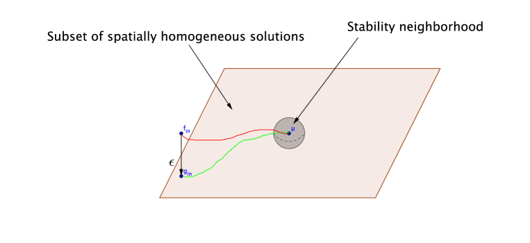
Figure 1. Sketch of the construction of weakly inhomogeneous solutions.

5.3. Proof of Theorem 5.3, part (I)

5.3.1. A priori moment bounds

Polynomial moments estimates are now a classical tool in the theory of the spatially homogeneous Boltzmann equation. Exponential moments estimates for the spatially homogeneous Boltzmann equation are more recent, see [16, 18, 41] and the references therein. In the latter references exponential moments (in integral or pointwise forms) are shown to be propagated. In the papers [69, 75, 65, 2] a theory of appearance of exponential moments was developed, still in the spatially homogeneous case. We shall extend this theory to the inhomogeneous framework, taking advantage of the a priori bounds on the solutions.

Lemma 5.9.

Consider for $T\in(0,+\infty]$ a conservative solution

$$0\leq f\in L^{1}_{t,loc}\left([0,T),L^{1}_{v}L^{\infty}_{x}(1+|v|^{2})\right)\cap C^{0}_{t}\left([0,T),L^{1}_{v}L^{\infty}_{x}(1+|v|)\right)$$

with initial datum bounded uniformly from below as in (5.1).

Then the solution $f$ has the following properties: for any $k>2$ and $T^{\prime}\in(0,T)$ there is an explicit constant $C(k,T^{\prime})>0$ depending on $k>2$, on the $L^{\infty}_{t}([0,T^{\prime}],L^{1}_{v}L^{\infty}_{x}(1+|v|))$ norm of the solution, on the lower bound (5.1) on the initial datum, and on $T^{\prime}$, so that

(5.5) $$\forall\,t\in(0,T^{\prime}],\quad\int_{{\mathbb{T}}^{3}\times{\mathbb{R}}^{3}}f_{t}(x,v)\,|v|^{k}{\,\mathrm{d}}x{\,\mathrm{d}}v\leq C(k,T^{\prime})\,\max\left\{\frac{1}{t^{k-2}},1\right\}.$$

Remark 5.10.

Observe that our moment estimate is not uniform in time. This is due to the lack of known uniform-in-time estimates from below on solutions to the nonlinear Boltzmann equation with such a low regularity. This will however not cause any problem for our uniform-in-time stability results since the “trapping mechanism” around the linearized regime takes over in finite time for the solutions we considered.

Proof of Lemma 5.9.

Using the Duhamel formulation and the above bounds on the solution we have for $T^{\prime}\in(0,T)$:

$$\forall\,t\geq\in[0,T^{\prime}],\ x\in{\mathbb{T}}^{3},\ v\in{\mathbb{R}}^{3},\\ f_{t}(x,v)=e^{-\int_{0}^{t}Q^{-}(f_{\tau},f_{\tau})(x-v(t-\tau),v){\,\mathrm{d}}\tau}\,f_{\mbox{{\scriptsize in}}}(x-vt,v)\\ +\int_{0}^{t}e^{-\int_{0}^{\tau}Q^{-}(f_{\tau^{\prime}},f_{\tau^{\prime}})(x-v(\tau-\tau^{\prime}),v){\,\mathrm{d}}\tau^{\prime}}\,Q^{+}(f_{\tau},f_{\tau})(x-v(t-\tau),v){\,\mathrm{d}}\tau\\ \geq e^{-c(T^{\prime})t(1+|v|)}\,\varphi(v)$$

for some constant $c(T^{\prime})>0$ depending on $T^{\prime}$ (through the $L^{\infty}_{t}([0,T^{\prime}],L^{1}_{v}L^{\infty}_{x}(1+|v|^{2}))$ norm of the solution).

We deduce that there is a constant $K(T^{\prime})>0$ so that

$$\forall\,t\in[0,T^{\prime}],\ x\in{\mathbb{T}}^{3},\ v\in{\mathbb{R}}^{3},\quad\int_{{\mathbb{R}}^{3}}f_{t}(x,v_{*})\,|v-v_{*}|{\,\mathrm{d}}v_{*}\geq K(T^{\prime})\,(1+|v|).$$

Consider now the moments of the solutions

$$M_{k}[f_{t}]:=\int_{{\mathbb{T}}^{3}\times{\mathbb{R}}^{3}}f_{t}(x,v)\,(1+|v|^{k})\,{\,\mathrm{d}}x{\,\mathrm{d}}v,\quad k\geq 0,$$

and apply the Lemma 4.5 to get for $k>2$ the following inequality in the sense of distribution

$${\frac{\mathrm{d}}{\mathrm{d}t}}M_{k}[f_{t}]=\int_{{\mathbb{T}}^{3}\times{\mathbb{R}}^{3}\times{\mathbb{R}}^{3}\times\mathbb{S}^{2}}f_{t}(x,v)\,f_{t}(x,v_{*})\\ \times\left[|v^{\prime}|^{k}+|v^{\prime}_{*}|^{k}-|v|^{k}-|v_{*}|^{k}\right]\,|v-v_{*}|{\,\mathrm{d}}v{\,\mathrm{d}}v_{*}{\,\mathrm{d}}\sigma{\,\mathrm{d}}x\\ \leq C_{k}\,\int_{{\mathbb{T}}^{3}\times{\mathbb{R}}^{3}\times{\mathbb{R}}^{3}}f_{t}(x,v)\,f_{t}(x,v_{*})\,(1+|v|^{k})\,(1+|v_{*}|^{2}){\,\mathrm{d}}x{\,\mathrm{d}}v\\ -2\,\int_{{\mathbb{T}}^{3}\times{\mathbb{R}}^{3}\times{\mathbb{R}}^{3}}f_{t}(x,v)\,f_{t}(x,v_{*})\,|v|^{k}\,|v-v_{*}|{\,\mathrm{d}}x{\,\mathrm{d}}v{\,\mathrm{d}}v_{*}\\ \leq C^{\prime}_{k}\,M_{k}[f_{t}]-K_{k}\,M_{k+1}[f_{t}]\leq C^{\prime}_{k}\,M_{k}[f_{t}]-K_{k}^{\prime}\,M_{k}^{\frac{k-1}{k-2}}[f_{t}]$$

for some constants $C_{k},C_{k}^{\prime},K_{k},K_{k}^{\prime}>0$ depending on the $L^{1}_{v}L^{\infty}_{x}(1+|v|^{2})$ upper bound on the solution and the previous lower bound. By standard interpolation and Gronwall inequality argument this leads to the bound

$$\forall\,t\in(0,T^{\prime}],\quad M_{k}[f_{t}]\leq\frac{C(k,T^{\prime})}{t^{k-2}}$$

for some constant $C(k,T^{\prime})>0$ which depends on $k>2$, $T^{\prime}>0$ and on the bounds on the solution. ∎

Lemma 5.11.

Consider for $T\in(0,+\infty]$ a conservative solution

$$0\leq f\in L^{1}_{t,loc}\left([0,T),L^{1}_{v}W^{3,1}_{x}(1+|v|^{2})\right)\cap C^{0}_{t}\left([0,T),L^{1}_{v}W^{3,1}_{x}(1+|v|)\right)$$

with initial datum bounded uniformly from below as in  (5.1).

Then for any $T^{\prime}\in(0,T)$, there exist explicit constants $\kappa,C>0$ (depending on the bounds assumed on the solution, on the lower bound (5.1) on the initial datum, and on $T^{\prime}>0$) such that

(5.6) $$\forall\,t\in[0,T^{\prime}],\quad{\left\|f_{t}\right\|}_{L^{1}_{v}W^{3,1}_{x}(e^{\kappa\min\{t,1\}|v|})}\leq C.$$

Proof of Lemma 5.11.

As a first step let us extend the polynomial moment bounds to the derivatives of the solution. Let us define

$$\tilde{M}_{k}(t):=\sum_{|\alpha|\leq 3}c_{\alpha}\,M_{k}[\partial_{x}^{\alpha}f_{t}]$$

for some constants $c_{\alpha}>0$ to be fixed later. Arguing as in the previous lemma and using the Sobolev embedding $W^{3,1}_{x}\hookrightarrow L^{\infty}_{x}$, we get

$${\frac{\mathrm{d}}{\mathrm{d}t}}M_{k}[f_{t}]\leq C^{\prime}_{k}\,M_{k}[f_{t}]-K_{k}^{\prime}\,M_{k}^{\frac{k-1}{k-2}}[f_{t}]$$

for some constants depending on time. For the first derivatives we write (with the notation $s=\mbox{sign}(\partial_{x}f)$)

$${\frac{\mathrm{d}}{\mathrm{d}t}}M_{k}[\partial_{x}f_{t}]=\int_{{\mathbb{T}}^{3}\times{\mathbb{R}}^{3}\times{\mathbb{R}}^{3}\times\mathbb{S}^{2}}\partial_{x}f_{t}(x,v)\,f_{t}(x,v_{*})\\ \times\left[|v^{\prime}|^{k}s^{\prime}+|v^{\prime}_{*}|^{k}s^{\prime}_{*}-|v|^{k}s-|v_{*}|^{k}s_{*}\right]\,|v-v_{*}|{\,\mathrm{d}}v{\,\mathrm{d}}v_{*}{\,\mathrm{d}}\sigma{\,\mathrm{d}}x\\ \leq C_{k}\,\int_{{\mathbb{T}}^{3}\times{\mathbb{R}}^{3}\times{\mathbb{R}}^{3}}|\partial_{x}f_{t}(x,v)|\,f_{t}(x,v_{*})\,(1+|v|^{k})\,(1+|v_{*}|^{2}){\,\mathrm{d}}x{\,\mathrm{d}}v\\ -2\,\int_{{\mathbb{T}}^{3}\times{\mathbb{R}}^{3}\times{\mathbb{R}}^{3}}|\partial_{x}f_{t}(x,v)|\,f_{t}(x,v_{*})\,|v|^{k}\,|v-v_{*}|{\,\mathrm{d}}x{\,\mathrm{d}}v{\,\mathrm{d}}v_{*}\\ +2\,\int_{{\mathbb{T}}^{3}\times{\mathbb{R}}^{3}\times{\mathbb{R}}^{3}}|\partial_{x}f_{t}(x,v)|\,f_{t}(x,v_{*})\,(1+|v|)\,(1+|v_{*}|^{k+1}){\,\mathrm{d}}x{\,\mathrm{d}}v{\,\mathrm{d}}v_{*}\\ \leq C_{k}\,M_{k}[\partial_{x}f_{t}]-K_{k}\,M_{k+1}[\partial_{x}f_{t}]+C\,M_{k+1}[f_{t}].$$

We calculate similarly for any $|\alpha|\leq 3$:

$${\frac{\mathrm{d}}{\mathrm{d}t}}M_{k}[\partial_{x}^{\alpha}f_{t}]\leq C_{k}\,M_{k}[\partial_{x}^{\alpha}f_{t}]-K_{k}\,M_{k+1}[\partial_{x}^{\alpha}f_{t}]+C\,\sum_{\beta<\alpha}M_{k+1}[\partial_{x}^{\beta}f_{t}].$$

Finally choosing suitable constants $c_{\alpha}>0$, we deduce

$${\frac{\mathrm{d}}{\mathrm{d}t}}\tilde{M}_{k}(t)\leq C_{k}^{\prime}\,\tilde{M}_{k}(t)-K_{k}^{\prime}\,\tilde{M}_{k+1}(t)\leq C_{k}^{\prime}\,\tilde{M}_{k}(t)-K_{k}^{\prime\prime}\,\tilde{M}_{k}(t)^{\frac{k-1}{k-2}}$$

which shows that

$$\forall\,t\in(0,T^{\prime}],\quad\tilde{M}_{k}(t)\leq C_{k}\,\max\left\{\frac{1}{t^{k-2}},1\right\}.$$

We now consider exponential moments and extend the argument in [2] to spatially inhomogeneous solutions in the torus. Our goal is to estimate the quantity

$$E(t,z):=\sum_{|\alpha|\leq 3}c_{\alpha}\int_{{\mathbb{T}}^{3}\times{\mathbb{R}}^{3}}\left|\partial_{x}^{\alpha}f_{t}(x,v)\right|\exp\big{(}z|v|\big{)}{\,\mathrm{d}}x{\,\mathrm{d}}v\\ =\sum_{|\alpha|\leq 3}c_{\alpha}\sum_{k=0}^{\infty}M_{k}[\partial_{x}^{\alpha}f_{t}]\frac{z^{k}}{k!}$$

where $z$ will depend on time. For use below let us define the truncated sum as

$$E^{n}(t,z):=\sum_{|\alpha|\leq 3}c_{\alpha}\sum_{k=0}^{n}M_{k}[\partial_{x}^{\alpha}f_{t}]\frac{z^{k}}{k!}$$

for $n\in\mathbb{N}$, $z\geq 0$, and $t\geq 0$. We also define

$$I^{n}(t,z):=\sum_{|\alpha|\leq 3}c_{\alpha}\sum_{k=0}^{n}M_{k+1}[\partial_{x}^{\alpha}f_{t}]\frac{z^{k}}{k!}$$

and

$$S_{\ell}(t):=\sum_{|\alpha|\leq 3}c_{\alpha}\sum_{k=1}^{k_{\ell}}{\ell\choose k}\left(M_{k+1}[\partial_{x}^{\alpha}f_{t}]M_{\ell-k}[\partial_{x}^{\alpha}f_{t}]+M_{k}[\partial_{x}^{\alpha}f_{t}]M_{\ell-k+1}[\partial_{x}^{\alpha}f_{t}]\right),$$

where $k_{\ell}$ is the integer part of $(\ell+1)/2$.

Let us prove the following inequality: there exists some constant $C>0$ independent of $n$ such that for any $\ell_{0}\geq 2$ the following holds:

(5.7) $$\sum_{\ell=\ell_{0}}^{n}\frac{z^{\ell}}{\ell!}S_{\ell}(t)\leq C\,E^{n}(t,z)\,I^{n}(t,z).$$

The first part of the sum in the left hand side of (5.7) can be bounded as:

$$\sum_{|\alpha|\leq 3}c_{\alpha}\sum_{\ell=\ell_{0}}^{n}\frac{z^{\ell}}{\ell!}\sum_{k=1}^{k_{\ell}}{\ell\choose k}M_{k+1}[\partial_{x}^{\alpha}f_{t}]M_{\ell-k}[\partial_{x}^{\alpha}f_{t}]\\ =\sum_{|\alpha|\leq 3}c_{\alpha}\sum_{\ell=\ell_{0}}^{n}\sum_{k=1}^{k_{\ell}}M_{k+1}[\partial_{x}^{\alpha}f_{t}]\,\frac{z^{k}}{k!}\,M_{\ell-k}[\partial_{x}^{\alpha}f_{t}]\,\frac{z^{\ell-k}}{(\ell-k)!}\\ \leq\sum_{|\alpha|\leq 3}c_{\alpha}\sum_{k=1}^{n}M_{k+1}[\partial_{x}^{\alpha}f_{t}]\,\frac{z^{k}}{k!}\sum_{\ell=\max\{\ell_{0},2k-1\}}^{n}M_{\ell-k}[\partial_{x}^{\alpha}f_{t}]\frac{z^{\ell-k}}{(\ell-k)!}\\ \leq C\,I^{n}(t,z)\,E^{n}(t,z).$$

We carry out a similar estimate for the other part:

$$\sum_{|\alpha|\leq 3}c_{\alpha}\sum_{\ell=\ell_{0}}^{n}\frac{z^{\ell}}{\ell!}\sum_{k=1}^{k_{\ell}}{\ell\choose k}M_{k}[\partial_{x}^{\alpha}f_{t}]M_{\ell-k+1}[\partial_{x}^{\alpha}f_{t}]\\ =\sum_{|\alpha|\leq 3}c_{\alpha}\sum_{\ell=\ell_{0}}^{n}\sum_{k=1}^{k_{\ell}}M_{k}[\partial_{x}^{\alpha}f_{t}]\,\frac{z^{k}}{k!}\,M_{\ell-k+1}[\partial_{x}^{\alpha}f_{t}]\,\frac{z^{\ell-k}}{(\ell-k)!}\\ \leq\sum_{|\alpha|\leq 3}c_{\alpha}\sum_{k=1}^{n}M_{k}[\partial_{x}^{\alpha}f_{t}]\,\frac{z^{k}}{k!}\sum_{\ell=\max\{\ell_{0},2k-1\}}^{n}M_{\ell-k+1}[\partial_{x}^{\alpha}f_{t}]\frac{z^{\ell-k}}{(\ell-k)!}\\ \leq C\,E^{n}(t,z)\,I^{n}(t,z).$$

This concludes the proof of (5.7).

First we notice that in order to prove (5.6) it is enough to prove the following: there are some constants $T_{0}\in(0,T)$ and $\kappa,C>0$ (which depend only on $b$ and the initial mass and energy) such that

(5.8) $${\left\|f_{t}\right\|}_{L^{1}_{v}W^{3,1}_{x}(e^{\kappa t|v|})}\leq C\quad\text{ for }t\in[0,T_{0}].$$

Indeed, since the assumptions are satisfied on the whole time interval $[0,T)$, for $t\geq T_{0}$ it is then possible to apply (5.8) starting at time $(t-T_{0})$.

Hence, we aim at proving the estimate (5.8). Let us denote

$$E_{0}=E^{n}(0,0)=E(0,0)={\left\|f_{\mbox{{\scriptsize in}}}\right\|}_{L^{1}_{v}W^{3,1}_{x}}.$$

Consider $\kappa>0$ to be fixed later, $n\in\mathbb{N}$ and define $T_{0}>0$ as

$$T_{0}:=\min\Big{\{}1\ ;\ \sup\big{\{}t>0\ \text{ s.t. }\ E^{n}(t,\kappa t)<4\,E_{0}\big{\}}\Big{\}}.$$

The definition is consistent and the previous polynomial moment estimates ensure that $T_{0}>0$ for each given $n$. The bound of $1$ is not essential, and is included just to ensure that $T_{0}$ is always finite. We note that a priori such $T_{0}$ depends on the index $n$ in the sum $E^{n}$ but we will prove a uniform bound on it.

Choose an integer $\ell_{0}\geq 3$, to be fixed later. Arguing as in [2], by classical functional inequalities we have

$$\forall\,t\in[0,T),\ \ell\geq\ell_{0},\quad{\frac{\mathrm{d}}{\mathrm{d}t}}M_{\ell}[f_{t}]\leq A_{\ell}\,S_{\ell}(t)-K\,M_{\ell+1}[f_{t}]$$

with $S_{\ell}$ defined as before, $K>0$ uniform, and $A_{\ell}$ positive decreasing and going to zero as $\ell\to\infty$. We can extend this argument to higher derivatives at the price of an additional error term as before:

$$\forall\,t\in[0,T),\ \ell\geq\ell_{0},\quad{\frac{\mathrm{d}}{\mathrm{d}t}}M_{\ell}[\partial^{\alpha}_{x}f_{t}]\\ \leq A_{\ell}\,S_{\ell}(t)-K\,M_{\ell+1}[\partial_{x}^{\alpha}f_{t}]+C\,\sum_{\beta<\alpha}M_{\ell+1}[\partial^{\beta}_{x}f_{t}].$$

By linear combination with careful choice of the constants $c_{\alpha}$ we deduce that

$$\forall\,t\in[0,T),\ \ell\geq\ell_{0},\quad{\frac{\mathrm{d}}{\mathrm{d}t}}\tilde{M}_{\ell}(t)\leq A_{\ell}\,S_{\ell}(t)-K\,\tilde{M}_{\ell+1}(t)$$

for some uniform $K>0$ and $A_{\ell}$ positive decreasing going to zero as $\ell\to 0$.

In addition, we know from the previous polynomial estimates that

(5.9) $$\forall\,t\in[0,T),\quad\sum_{\ell=0}^{\ell_{0}}\tilde{M}_{\ell}(t)\,t^{\ell}\leq C_{\ell_{0}}.$$

Taking any $\kappa\in(0,1)$ and using the product rule we get:

$$\frac{\mathrm{d}}{\mathrm{d}t}\sum_{\ell=\ell_{0}}^{n}\tilde{M}_{\ell}(t)\,\frac{(\kappa t)^{\ell}}{\ell!}\\ \leq\sum_{\ell=\ell_{0}}^{n}\frac{(\kappa t)^{\ell}}{\ell!}\left(A_{\ell}\,S_{\ell}(t)-K\,\tilde{M}_{\ell+1}(t)\right)+\kappa\,\sum_{\ell=\ell_{0}}^{n}\tilde{M}_{\ell}(t)\,\frac{(\kappa t)^{\ell-1}}{(\ell-1)!}\\ \leq\sum_{\ell=\ell_{0}}^{n}\frac{(at)^{\ell}}{\ell!}A_{\ell}\,S_{\ell}(t)+(\kappa-K)\,I^{n}(t,\kappa t)+(K+\kappa)\,\sum_{\ell=1}^{\ell_{0}}\tilde{M}_{\ell}(t)\,\frac{(\kappa t)^{\ell-1}}{(\ell-1)!}\\ \leq\sum_{\ell=\ell_{0}}^{n}\frac{(\kappa t)^{\ell}}{\ell!}A_{\ell}\,S_{\ell}+(\kappa-K)\,I^{n}(t,\kappa t)+\frac{(K+\kappa)}{t}\,C_{\ell_{0}},$$

where we have used that $\kappa<1$ and inequality (5.9) in the last step. Hence, from the inequality (5.7) we obtain

$$\frac{\mathrm{d}}{\mathrm{d}t}\sum_{\ell=\ell_{0}}^{n}\tilde{M}_{\ell}(t)\frac{(\kappa t)^{\ell}}{\ell!}\leq I^{n}(t,\kappa t)\Big{[}C\,A_{\ell_{0}}\,E^{n}(t,\kappa t)+(\kappa-K)\Big{]}+\frac{(K+\kappa)}{t}\,C_{\ell_{0}}.$$

Next, choose $\kappa\leq\min\{1,K/2\}$ and $\ell_{0}$ large enough so that

$$\forall\,t\in[0,T_{0}],\quad C\,A_{\ell_{0}}\,E^{n}(t,\kappa t)\leq C\,A_{\ell_{0}}\,4\,E_{0}\leq\frac{K}{4}.$$

Hence

(5.10) $$\frac{\mathrm{d}}{\mathrm{d}t}\sum_{\ell=\ell_{0}}^{n}\tilde{M}_{\ell}(t)\frac{(\kappa t)^{\ell}}{\ell!}\leq-\frac{K}{4}\,I^{n}(t,\kappa t)+\frac{(K+\kappa)}{t}\,C_{\ell_{0}}\\ \leq-\frac{1}{t}\left[\frac{K}{4\kappa}\left(E^{n}(t,\kappa t)-E_{0}\right)-(K+\kappa)\,C_{\ell_{0}}\right]$$

where for the last inequality we have used that (thanks to the conservation of the total mass)

$$I^{n}(t,\kappa t)\geq\frac{(E^{n}(t,\kappa t)-E_{0})}{\kappa t}.$$

We make the additional restriction that $\kappa<E_{0}/(6C_{\ell_{0}})$, which together with $\kappa\leq\min\{1,K/2\}$ implies that

$$\frac{K}{4\kappa}\,E_{0}>(K+\kappa)\,C_{\ell_{0}}.$$

Then we have

(5.11) $$\frac{\mathrm{d}}{\mathrm{d}t}\sum_{\ell=\ell_{0}}^{n}\tilde{M}_{\ell}(t)\frac{(\kappa t)^{\ell}}{\ell!}\leq 0$$

for any time $t\in[0,T_{0}]$ for which $E^{n}(t,\kappa t)\geq 2\,E_{0}$ holds. This is true in particular when $\sum_{\ell=\ell_{0}}^{n}\tilde{M}_{\ell}(t)\,\frac{(\kappa t)^{\ell}}{\ell!}\geq 2\,E_{0}$. We deduce that

(5.12) $$\forall\,t\in[0,T_{0}],\quad\sum_{\ell=\ell_{0}}^{n}\tilde{M}_{\ell}\frac{(\kappa t)^{\ell}}{\ell!}\leq 2\,E_{0}.$$

In order to finish the argument we need to bound the initial part of the full sum (from $\ell=0$ to $\ell_{0}-1$.) Indeed, we note that from (5.9),

(5.13) $$\forall\,t\in[0,T_{0}],\quad\sum_{\ell=0}^{\ell_{0}-1}\tilde{M}_{\ell}(t)\,\frac{(\kappa t)^{\ell}}{\ell!}\leq E_{0}+\kappa\,C_{\ell_{0}},$$

so, recalling that $6\kappa C_{\ell_{0}}<E_{0}$ and using (5.12) and (5.13) we get

$$E^{n}(t,\kappa t)=\sum_{\ell=0}^{\ell_{0}-1}\tilde{M}_{\ell}(t)\,\frac{(\kappa t)^{\ell}}{\ell!}+\sum_{\ell=\ell_{0}}^{n}\tilde{M}_{\ell}(f)\,\frac{(\kappa t)^{\ell}}{\ell!}\leq 3\,E_{0}+\kappa\,C_{\ell_{0}}\leq\frac{19}{6}\,E_{0}$$

for $t\in[0,T_{0}]$, uniformly in $n$. Finally, gathering all conditions imposed along the proof on the parameter $\kappa$, we choose

(5.14) $$\kappa:=\min\left\{1,\frac{K}{2},\frac{E_{0}}{6C_{\ell_{0}}}\right\}$$

independently of $n$. We conclude, from the definition of $T_{0}$, that $T_{0}=1$ for all $n$. Sending $n\rightarrow\infty$, we deduce the result. ∎

5.3.2. Non appearance of “superlinear” exponential moments

Lemma 5.12.

Consider for $T\in(0,+\infty]$ a conservative solution

$$0\leq f\in L^{1}_{t,loc}\left([0,T),L^{1}_{v}W^{3,1}_{x}(1+|v|^{2})\right)\cap C^{0}_{t}\left([0,T),L^{1}_{v}W^{3,1}_{x}(1+|v|)\right)$$

with initial datum bounded uniformly from below as in  (5.1). Assume that for $\beta\in(1,2]$ the initial condition satisfies

$$\forall\,\kappa>0,\quad{\left\|f_{\mbox{{\scriptsize{\em in}}}}\right\|}_{L^{1}_{v}W^{3,1}_{x}(e^{\kappa\,|v|^{\beta}})}=+\infty.$$

Then we have

$$\forall\,t\geq 0,\ \forall\,\kappa>0,\quad{\left\|f_{t}\right\|}_{L^{1}_{v}W^{3,1}_{x}(e^{\kappa\,|v|^{\beta}})}=+\infty.$$

Proof of Lemma 5.12.

We only sketch the proof in the case $\beta=2$ and leave to the reader the general case. The key idea is to define

$$E^{n}_{R}(t,z):=\sum_{|\alpha|\leq 3}c_{\alpha}\sum_{k=0}^{n}\left(\int_{{\mathbb{T}}^{3}\times{\mathbb{R}}^{3}}\left|\partial_{x}^{\alpha}f_{t}\right|\,(1+|v|)^{2k}\,{\bf 1}_{|v|\leq R}\,{\,\mathrm{d}}x{\,\mathrm{d}}v\right)\frac{z^{k}}{k!}$$

for some parameter $R>0$, and then consider $E^{n}_{R}(t,\kappa(1+\kappa^{\prime}t))$ with $\kappa$ arbitrary and $\kappa^{\prime}$ to be fixed later. Observe that $E^{n}_{R}(t,z)$ is always well-defined and finite for all time and value of $z$ due to the truncations. We calculate (dropping out the positive terms)

$${\frac{\mathrm{d}}{\mathrm{d}t}}E^{n}_{R}\left(t,\kappa(1+\kappa^{\prime}t)\right)\\ \geq-K\,\sum_{|\alpha|\leq 3}c_{\alpha}\sum_{k=0}^{n}\left(\int_{{\mathbb{T}}^{3}\times{\mathbb{R}}^{3}}\left|\partial_{x}^{\alpha}f_{t}\right|\,{\bf 1}_{|v|\leq R}\,(1+|v|)^{2k+1}\,{\,\mathrm{d}}x{\,\mathrm{d}}v\right)\,\frac{\left(\kappa(1+\kappa^{\prime}t)\right)^{k}}{k!}\\ +\kappa\kappa^{\prime}\,\sum_{|\alpha|\leq 3}c_{\alpha}\sum_{k=1}^{n}\left(\int_{{\mathbb{T}}^{3}\times{\mathbb{R}}^{3}}\left|\partial_{x}^{\alpha}f_{t}\right|\,{\bf 1}_{|v|\leq R}\,(1+|v|)^{2k}\,{\,\mathrm{d}}x{\,\mathrm{d}}v\right)\,\frac{\left(\kappa(1+\kappa^{\prime}t)\right)^{k-1}}{(k-1)!}.$$

We deduce that for $\kappa^{\prime}$ large enough

$${\frac{\mathrm{d}}{\mathrm{d}t}}E^{n}_{R}\left(t,\kappa(1+\kappa^{\prime}t)\right)\\ \geq-K\,\sum_{|\alpha|\leq 3}c_{\alpha}\left(\int_{{\mathbb{T}}^{3}\times{\mathbb{R}}^{3}}\left|\partial_{x}^{\alpha}f_{t}\right|\,{\bf 1}_{|v|\leq R}\,(1+|v|)^{2n+1}\,{\,\mathrm{d}}x{\,\mathrm{d}}v\right)\,\frac{\left(\kappa(1+\kappa^{\prime}t)\right)^{n}}{n!}.$$

Since the right hand side goes to zero as $n\to+\infty$ we deduce the a priori estimate

$${\frac{\mathrm{d}}{\mathrm{d}t}}E_{R}^{\infty}\left(t,\kappa(1+\kappa^{\prime}t)\right)\geq 0.$$

We hence deduce by passing to the limit $R\to\infty$ that $E^{\infty}_{\infty}(t,\kappa(1+\kappa^{\prime}t))=+\infty$ for $t\geq 0$ which concludes the proof. ∎

5.3.3. A priori lower bounds

The proof of the Maxwellian lower bound in part (I) of Theorem 5.3 is a straightforward application of [73] and we shall therefore skip the proof. In the paper [73] an a priori bound was assumed on the entropy but it can be removed using the non-concentration estimates on the iterated gain term first discovered in [70] and then developed in [1]. We refer to the more recent preprint [23] where these issues are discussed.

5.3.4. A priori uniqueness for conservative solutions

This subsection is related to the Cauchy theory for unique solution to the spatially homogeneous Boltzmann for hard spheres in $L^{1}_{v}(1+|v|^{2})$. Let us refer first to [33] for the idea of the key a priori estimate on moment of the difference of two solutions and [5, 6] for the first uniqueness result in a space of the form $L^{1}_{v}(1+|v|^{k})$ (with $k>2$). Then we refer to [70, 63] (and later [65] following the same approach) for the more recent optimal results. In these papers, there are mainly two approaches. The first one [70] relies on a subtle variants of the Povzner inequality, and the second one [63] (see also [65]) is more direct and relies on the estimate of the tail of the distribution at initial times. We shall elaborate upon this second approach in this subsection.

Lemma 5.13 (A priori uniqueness in $L^{1}_{v}L^{\infty}_{x}(1+|v|^{k})$, $k>2$).

Consider for $T\in(0,+\infty]$ and $k>2$ two conservative distributional solutions

$$f_{t},g_{t}\in L^{1}_{t,loc}\left([0,T),L^{1}_{v}L^{\infty}_{x}(1+|v|^{k})\right)\cap C^{0}_{t}\left([0,T),L^{1}_{v}L^{\infty}(1+|v|^{k-1})\right)$$

with initial data $f_{\mbox{{\scriptsize{\em in}}}},g_{\mbox{{\scriptsize{\em in}}}}$ satisfying the lower bound assumption (5.1). Then for any $T^{\prime}\in[0,T)$ there is some constant $C(T^{\prime})>0$ (depending on the bounds assumed on the solutions, on the lower bound (5.1) on the initial datum, and on $T^{\prime}>0$) such that

(5.15) $$\forall\,t\in[0,T^{\prime}],\quad{\left\|f_{t}-g_{t}\right\|}_{L^{1}_{x,v}(1+|v|^{2})}\leq C(T^{\prime})\,{\left\|f_{\mbox{{\scriptsize{\em in}}}}-g_{\mbox{{\scriptsize{\em in}}}}\right\|}_{L^{1}_{x,v}(1+|v|^{2})}.$$

Proof of Lemma 5.13.

Arguing as before we get

$$\forall\,t\in[0,T^{\prime}],\quad\int_{{\mathbb{R}}^{3}}f_{t}(x,v_{*})\,|v-v_{*}|{\,\mathrm{d}}v_{*}\geq K(T^{\prime})\,(1+|v|)$$

for some constant depending on the $L^{\infty}_{t}([0,T^{\prime}],L^{1}_{v}L^{\infty}(1+|v|^{k-1}))$ norm of $f$ and the lower bound (5.1) on $f_{\mbox{{\scriptsize in}}}$.

We then write the estimate (arguing as in the previous section)

$$\forall\,t\in[0,T^{\prime}],\quad{\frac{\mathrm{d}}{\mathrm{d}t}}{\left\|f_{t}\right\|}_{L^{1}_{v}L^{\infty}_{x}(1+|v|^{k})}\\ \leq C\,{\left\|f_{t}\right\|}_{L^{1}_{v}L^{\infty}_{x}(1+|v|^{2})}\,{\left\|f_{t}\right\|}_{L^{1}_{v}L^{\infty}_{x}(1+|v|^{k})}-K\,{\left\|f_{t}\right\|}_{L^{1}_{v}L^{\infty}_{x}(1+|v|^{k+1})}$$

which shows that ${\left\|f_{t}\right\|}_{L^{1}_{v}L^{\infty}_{x}(1+|v|^{3})}$ is time-integrable. Similarly we deduce that ${\left\|g_{t}\right\|}_{L^{1}_{v}L^{\infty}_{x}(1+|v|^{3})}$ is time-integrable on $[0,T^{\prime}]$. Finally we obtain the continuity of the flow in the topology $L^{1}_{v}L^{\infty}_{x}(1+|v|^{2})$:

$${\frac{\mathrm{d}}{\mathrm{d}t}}{\left\|f_{t}-g_{t}\right\|}_{L^{1}_{v}L^{\infty}_{x}(1+|v|^{2})}\\ \leq C\,\left({\left\|f_{t}\right\|}_{L^{1}_{v}L^{\infty}_{x}(1+|v|^{3})}+{\left\|g_{t}\right\|}_{L^{1}_{v}L^{\infty}_{x}(1+|v|^{3})}\right)\,{\left\|f_{t}-g_{t}\right\|}_{L^{1}_{v}L^{\infty}_{x}(1+|v|^{2})}$$

and thus

$$\forall\,t\in[0,T^{\prime}],\quad{\left\|f_{t}-g_{t}\right\|}_{L^{1}_{v}L^{\infty}_{x}(1+|v|^{2})}\\ \leq C\,e^{\int_{0}^{t}\left({\left\|f_{\tau}\right\|}_{L^{1}_{v}L^{\infty}_{x}(1+|v|^{3})}+{\left\|g_{\tau}\right\|}_{L^{1}_{v}L^{\infty}_{x}(1+|v|^{3})}\right){\,\mathrm{d}}\tau}\,{\left\|f_{\mbox{{\scriptsize in}}}-g_{\mbox{{\scriptsize in}}}\right\|}_{L^{1}_{v}L^{\infty}_{x}(1+|v|^{2})}$$

and the claimed uniqueness property follows. ∎

The next lemma follows an idea first introduced for the spatially homogeneous Boltzmann equation in [70, 63], using the reformulation in [65].

Lemma 5.14 (A priori uniqueness in the critical case $k=2$).

Consider for $T\in(0,+\infty]$ two conservative distributional solutions

$$f_{t},g_{t}\in L^{1}_{t,loc}\left([0,T),L^{1}_{v}W^{3,1}_{x}(1+|v|^{2})\right)\cap C^{0}_{t}\left([0,T),L^{1}_{v}W^{3,1}_{x}(1+|v|)\right)$$

with initial data $f_{\mbox{{\scriptsize{\em in}}}},g_{\mbox{{\scriptsize{\em in}}}}$ satisfying the lower bound assumption (5.1).

Then for any $T^{\prime}\in(0,T)$, there is an explicit function $\Psi:{\mathbb{R}}_{+}\to{\mathbb{R}}_{+}$ which depends on $T^{\prime}>0$, $f_{\mbox{{\scriptsize{\em in}}}}$ and $g_{\mbox{{\scriptsize{\em in}}}}$, which is continuous and satisfies $\Psi(0)=0$ and $\Psi(r)>0$ for $r>0$, such that

(5.16) $$\forall\,t\in[0,T^{\prime}],\quad{\left\|f_{t}-g_{t}\right\|}_{L^{1}_{x,v}(1+|v|^{2})}\leq\Psi\left({\left\|f_{\mbox{{\scriptsize{\em in}}}}-g_{\mbox{{\scriptsize{\em in}}}}\right\|}_{L^{1}_{x,v}(1+|v|^{2})}\right).$$

Proof of Lemma 5.14.

We fix $T^{\prime}\in(0,T)$ for the whole proof. Arguing exactly as in the first part of Lemma 5.9, we deduce that there is a constant $K(T^{\prime})>0$ so that

$$\forall\,t\in[0,T^{\prime}],\ x\in{\mathbb{T}}^{3},\ v\in{\mathbb{R}}^{3},\quad\left\{\begin{array}[]{l}\displaystyle\int_{{\mathbb{R}}^{3}}f_{t}(x,v_{*})\,|v-v_{*}|{\,\mathrm{d}}v_{*}\geq K(T^{\prime})\,(1+|v|),\vspace{0.3cm}\\ \displaystyle\int_{{\mathbb{R}}^{3}}g_{t}(x,v_{*})\,|v-v_{*}|{\,\mathrm{d}}v_{*}\geq K(T^{\prime})\,(1+|v|),\end{array}\right.$$

and

$$\forall\,t\in(0,T^{\prime}],\quad\left\{\begin{array}[]{l}\displaystyle\tilde{M}_{k}(t)\leq C_{k}(T^{\prime})\,\min\left\{\frac{1}{t^{k-2}},1\right\}\vspace{0.3cm}\\ \displaystyle\tilde{M}_{k}(t)\leq C_{k}(T^{\prime})\,\min\left\{\frac{1}{t^{k-2}},1\right\}\end{array}\right.$$

for some constant $C_{k}(T^{\prime})$ depending on $T^{\prime}>0$ and $k>2$, and where $\tilde{M}_{k}$ was defined in the proof of Lemma 5.9 (recall that it involves the derivatives $\partial_{x}^{\alpha}$, $|\alpha|\leq 3$).

Let us denote $d_{t}:=f_{t}-g_{t}$ and $s_{t}:=f_{t}+g_{t}$.

We have by usual calculations

$${\frac{\mathrm{d}}{\mathrm{d}t}}\int_{{\mathbb{T}}^{3}\times{\mathbb{R}}^{3}}|d_{t}|\,(1+|v|^{2}){\,\mathrm{d}}x{\,\mathrm{d}}v\\ \leq C\,\left(\int_{{\mathbb{T}}^{3}\times{\mathbb{R}}^{3}}|d_{t}|{\,\mathrm{d}}x{\,\mathrm{d}}v\right)\,\left(\sup_{x\in{\mathbb{T}}^{3}}\int_{{\mathbb{R}}^{3}}|s_{t}|\,(1+|v|^{3}){\,\mathrm{d}}v\right)\\ +C\,\,\left(\int_{{\mathbb{T}}^{3}\times{\mathbb{R}}^{3}}|d_{t}|\,(1+|v|){\,\mathrm{d}}x{\,\mathrm{d}}v\right)\,\left(\sup_{x\in{\mathbb{T}}^{3}}\int_{{\mathbb{R}}^{3}}|s_{t}|\,(1+|v|^{2}){\,\mathrm{d}}v\right)\\ \leq C_{1}\,\min\left\{\frac{1}{t},1\right\}\,\left(\int_{{\mathbb{T}}^{3}\times{\mathbb{R}}^{3}}|d_{t}|{\,\mathrm{d}}x{\,\mathrm{d}}v\right)+C_{2}\,\left(\int_{{\mathbb{T}}^{3}\times{\mathbb{R}}^{3}}|d_{t}|\,(1+|v|){\,\mathrm{d}}x{\,\mathrm{d}}v\right)$$

which provides a simple Gronwall-like estimates for times bounded away from zero.

Let us now consider small times. Define

$$r:=\min\left\{{\left\|d_{\mbox{{\scriptsize in}}}\right\|}_{L^{1}_{x,v}(1+|v|^{2})}\,;\,T^{\prime}\right\}$$

and let us estimate the $L^{1}_{x,v}(1+|v|^{2})$ norm of the difference for the times $t\in[0,r]$. Then calculate

$$\forall\,t\in[0,r],\quad{\left\|d_{t}\right\|}_{L^{1}_{x,v}(1+|v|^{2})}\\ \leq\int_{{\mathbb{T}}^{3}\times{\mathbb{R}}^{3}}d_{t}\,(1+|v|^{2}){\,\mathrm{d}}x{\,\mathrm{d}}v+2\,\int_{{\mathbb{T}}^{3}\times{\mathbb{R}}^{3}}(d_{t})_{+}\,(1+|v|^{2}){\,\mathrm{d}}x{\,\mathrm{d}}v\\ \leq\int_{{\mathbb{T}}^{3}\times{\mathbb{R}}^{3}}d_{\mbox{{\scriptsize in}}}\,(1+|v|^{2}){\,\mathrm{d}}x{\,\mathrm{d}}v+2\,\int_{{\mathbb{T}}^{3}\times{\mathbb{R}}^{3}}f_{t}\,(1+|v|^{2}){\,\mathrm{d}}x{\,\mathrm{d}}v\\ \leq\int_{{\mathbb{T}}^{3}\times{\mathbb{R}}^{3}}|d_{\mbox{{\scriptsize in}}}|\,(1+|v|^{2}){\,\mathrm{d}}x{\,\mathrm{d}}v+2\,\int_{{\mathbb{T}}^{3}\times{\mathbb{R}}^{3}}f_{t}\,(1+|v|^{2}){\,\mathrm{d}}x{\,\mathrm{d}}v\\ \leq r+2\,\int_{|v|\leq R}f_{t}\,(1+|v|^{2}){\,\mathrm{d}}x{\,\mathrm{d}}v+2\,\int_{|v|>R}f_{t}\,(1+|v|^{2}){\,\mathrm{d}}x{\,\mathrm{d}}v\\ \leq r+2\,(1+R^{2})\,{\left\|d_{t}\right\|}_{L^{1}_{x,v}}+2\,\int_{|v|>R}f_{t}\,(1+|v|^{2}){\,\mathrm{d}}x{\,\mathrm{d}}v$$

for some parameter $R>0$ to be chosen later, where we have used the conservation of the energy of our solutions and the inequality $(d_{t})_{+}\leq f_{t}$.

The second term in the right hand side above can be estimated as

$${\frac{\mathrm{d}}{\mathrm{d}t}}\int_{{\mathbb{T}}^{3}\times{\mathbb{R}}^{3}}|d_{t}|{\,\mathrm{d}}x{\,\mathrm{d}}v\leq C\,\int_{{\mathbb{T}}^{3}\times{\mathbb{R}}^{3}}d_{t}(s_{t})_{*}\,|v-v_{*}|{\,\mathrm{d}}x{\,\mathrm{d}}v{\,\mathrm{d}}v_{*}\\ \leq C^{\prime}\,\left(\int_{{\mathbb{T}}^{3}\times{\mathbb{R}}^{3}}|d_{t}|\,(1+|v|){\,\mathrm{d}}x{\,\mathrm{d}}v\right).$$

Hence

$$\forall\,t\in[0,r],\quad{\left\|d_{t}\right\|}_{L^{1}_{x,v}}\\ \leq{\left\|d_{\mbox{{\scriptsize in}}}\right\|}_{L^{1}_{x,v}(1+|v|^{2})}+C^{\prime}\,\int_{0}^{t}\left({\left\|f_{\tau}\right\|}_{L^{1}_{x,v}(1+|v|^{2})}{\left\|g_{\tau}\right\|}_{L^{1}_{x,v}(1+|v|^{2})}\right){\,\mathrm{d}}\tau\leq C^{\prime\prime}\,r.$$

Finally the third term of the right hand side can be estimated as

$$\int_{|v|>R}f_{t}\,(1+|v|^{2}){\,\mathrm{d}}x{\,\mathrm{d}}v=\int_{{\mathbb{T}}^{3}\times{\mathbb{R}}^{3}}f_{t}\,(1+|v|^{2}){\,\mathrm{d}}x{\,\mathrm{d}}v-\int_{|v|\leq R}f_{t}\,(1+|v|^{2}){\,\mathrm{d}}x{\,\mathrm{d}}v\\ =\int_{{\mathbb{T}}^{3}\times{\mathbb{R}}^{3}}f_{\mbox{{\scriptsize in}}}\,(1+|v|^{2}){\,\mathrm{d}}x{\,\mathrm{d}}v-\int_{|v|\leq R}f_{t}\,(1+|v|^{2}){\,\mathrm{d}}x{\,\mathrm{d}}v\\ =\int_{{\mathbb{T}}^{3}\times{\mathbb{R}}^{3}}f_{\mbox{{\scriptsize in}}}\,(1+|v|^{2}){\,\mathrm{d}}x{\,\mathrm{d}}v-\int_{|v|\leq R}f_{\mbox{{\scriptsize in}}}\,(1+|v|^{2}){\,\mathrm{d}}x{\,\mathrm{d}}v\\ -\int_{0}^{t}\int_{|v|\leq R}Q(f_{\tau},f_{\tau})\,(1+|v|^{2}){\,\mathrm{d}}x{\,\mathrm{d}}v{\,\mathrm{d}}\tau\\ \leq\int_{|v|>R}f_{\mbox{{\scriptsize in}}}\,(1+|v|^{2}){\,\mathrm{d}}x{\,\mathrm{d}}v+\int_{0}^{t}\int_{|v|\leq R}Q^{-}(f_{\tau},f_{\tau})\,(1+|v|^{2}){\,\mathrm{d}}x{\,\mathrm{d}}v{\,\mathrm{d}}\tau\\ \leq\int_{|v|>R}f_{\mbox{{\scriptsize in}}}\,(1+|v|^{2}){\,\mathrm{d}}x{\,\mathrm{d}}v+C^{\prime\prime\prime}\,r\,(1+R^{2})$$

where we have used again the conservation of energy and the evolution equation integrated against $(1+|v|^{2})\,{\bf 1}_{|v|\leq R}$.

Combining the three estimates we deduce that

$$\forall\,t\in[0,r],\quad{\left\|d_{t}\right\|}_{L^{1}_{x,v}(1+|v|^{2})}\leq\\ r+2\,C^{\prime\prime}\,r\,(1+R^{2})+2\,\int_{|v|>R}f_{\mbox{{\scriptsize in}}}\,(1+|v|^{2}){\,\mathrm{d}}x{\,\mathrm{d}}v+C^{\prime\prime\prime}\,r\,(1+R^{2}).$$

We finally choose for instance $R=r^{-1/3}$ and define

$$\Psi_{0}(r):=r+2\,C^{\prime\prime}\,r\,\left(1+r^{-2/3}\right)\\ +2\,\int_{|v|>r^{-1/3}}f_{\mbox{{\scriptsize in}}}\,(1+|v|^{2}){\,\mathrm{d}}x{\,\mathrm{d}}v+C^{\prime\prime\prime}\,r\,\left(1+r^{-2/3}\right)$$

which depends on the profiles $f_{\mbox{{\scriptsize in}}}$ and $g_{\mbox{{\scriptsize in}}}$ via the tail estimate in the right hand side and also via the constants depending on the mass and energy.

We have therefore

$$\forall\,t\in[0,r],\quad{\left\|d_{t}\right\|}_{L^{1}_{x,v}(1+|v|^{2})}\leq\Psi_{0}\left(r\right).$$

To conclude with the final stability estimate in the case $r<T^{\prime}$, we write

$$\forall\,t\in[0,T^{\prime}],\quad{\left\|d_{t}\right\|}_{L^{1}_{x,v}(1+|v|^{2})}\\ \leq{\left\|d_{r}\right\|}_{L^{1}_{x,v}(1+|v|^{2})}+\int_{r}^{t}\left(\frac{{\rm d}}{{\rm d}\tau}{\left\|d_{\tau}\right\|}_{L^{1}_{x,v}(1+|v|^{2})}\right){\,\mathrm{d}}\tau\\ \leq\Psi_{0}\left(r\right)+\int_{r}^{t}\left(C_{1}\,\min\left\{\frac{1}{\tau},1\right\}\,{\left\|d_{\tau}\right\|}_{L^{1}_{x,v}}+C_{2}\,{\left\|d_{\tau}\right\|}_{L^{1}_{x,v}(1+|v|)}\right){\,\mathrm{d}}\tau.$$

If $T^{\prime}\geq r\geq 1$ the proof is clear by a Gronwall estimate, for $r<1$ we write first (assuming $T^{\prime}\geq 1$ for notational simplicity, the case $T^{\prime}<1$ is similar)

$$\forall\,t\in[0,T^{\prime}],\quad{\left\|d_{t}\right\|}_{L^{1}_{x,v}(1+|v|^{2})}\leq\Psi_{0}\left(r\right)\\ +C_{1}\,\int_{r}^{1}{\left\|d_{\tau}\right\|}_{L^{1}_{x,v}}\frac{{\,\mathrm{d}}\tau}{\tau}+(C_{1}+2C_{2})\,\int_{1}^{T^{\prime}}{\left\|d_{\tau}\right\|}_{L^{1}_{x,v}(1+|v|^{2})}{\,\mathrm{d}}\tau$$

and for the second term of the right hand side we use the estimate on ${\left\|d_{\tau}\right\|}_{L^{1}_{x,v}}$:

$$\int_{r}^{1}{\left\|d_{\tau}\right\|}_{L^{1}_{x,v}}\frac{{\,\mathrm{d}}\tau}{\tau}\leq\int_{r}^{1}\left({\left\|d_{\mbox{{\scriptsize in}}}\right\|}_{L^{1}_{x,v}}+C\,\int_{0}^{\tau}{\left\|d_{\tau^{\prime}}\right\|}_{L^{1}_{x,v}}{\,\mathrm{d}}\tau^{\prime}\right)\frac{{\,\mathrm{d}}\tau}{\tau}\\ \leq r|\ln r|+C\,\int_{0}^{1}{\left\|d_{\tau^{\prime}}\right\|}_{L^{1}_{x,v}}\,|\ln\tau^{\prime}|{\,\mathrm{d}}\tau^{\prime}.$$

We thus deduce

$$\forall\,t\in[0,T^{\prime}],\quad{\left\|d_{t}\right\|}_{L^{1}_{x,v}(1+|v|^{2})}\leq\Psi_{0}\left(r\right)+r|\ln r|\\ +C_{1}^{\prime}\,\int_{0}^{1}{\left\|d_{\tau}\right\|}_{L^{1}_{x,v}}\,|\ln\tau|{\,\mathrm{d}}\tau+C_{2}^{\prime}\,\int_{1}^{T^{\prime}}{\left\|d_{\tau}\right\|}_{L^{1}_{x,v}(1+|v|^{2})}{\,\mathrm{d}}\tau$$

which yields the result for some nonlinear function $\Psi=\Psi(r)$ by the Gronwall lemma. ∎

5.4. Proof of Theorem 5.3, parts (II) and (III)

5.4.1. A dissipative Banach norm

In this subsection we construct a Banach norm for which the semigroup is not only dissipative, but also has a stronger dissipativity property: the damping term in the energy estimate controls the norm of the graph of the collision operator.

Observe that in this theorem, the rate of decay is possibly worse than in Theorem 4.2. It shall not however cause any problem when searching for the rate of decay of the nonlinear equation, as the latter can be recovered by a bootstrap argument once the stability is proved.

Proposition 5.15.

Consider the space ${\mathcal{E}}=W^{\sigma,q}_{v}W^{s,p}_{x}(m)$ with the same assumptions as in Theorem 4.2, with a norm denoted by $\|\cdot\|_{\mathcal{E}}$, and define the equivalent norm

(5.17) $$|\hskip-1.13791pt|\hskip-1.13791pt|h|\hskip-1.13791pt|\hskip-1.13791pt|_{{\mathcal{E}}}:=\eta\,\|h\|_{{\mathcal{E}}}+\int_{0}^{+\infty}\left\|S_{{\mathcal{L}}}(\tau)h\right\|_{{\mathcal{E}}}{\,\mathrm{d}}\tau,\quad\eta>0.$$

Then there exists $\eta>0$ (small enough) and $\lambda_{1}\in(0,\lambda)$ such that for any $h_{\mbox{{\scriptsize{\em in}}}}\in{\mathcal{E}}$, $\Pi h_{\mbox{{\scriptsize{\em in}}}}=0$ (let us recall that $\Pi$ is the projection on the eigenspace associated to the eigenvalue $0$ thanks to the formulas (2.1) and (4.7)), the solution $h(t):=S_{\mathcal{L}}(t)h_{\mbox{{\scriptsize{\em in}}}}$ to the linearized flow (4.5) satisfies:

$$\forall\,t\geq 0,\quad{{\rm d}\over{\rm d}t}|\hskip-1.13791pt|\hskip-1.13791pt|h_{t}|\hskip-1.13791pt|\hskip-1.13791pt|_{\mathcal{E}}\leq-\lambda_{1}\,|\hskip-1.13791pt|\hskip-1.13791pt|h_{t}|\hskip-1.13791pt|\hskip-1.13791pt|_{{\mathcal{E}}_{\nu}},$$

where

$${\mathcal{E}}_{\nu}:=W^{\sigma,q}_{v}W^{s,p}_{x}(\nu^{1/q}\,m)\subset{\mathcal{E}}$$

and $|\hskip-1.13791pt|\hskip-1.13791pt|\cdot|\hskip-1.13791pt|\hskip-1.13791pt|_{{\mathcal{E}}_{\nu}}$ is defined from $\|\cdot\|_{{\mathcal{E}}_{\nu}}$ as in (5.17):

$$|\hskip-1.13791pt|\hskip-1.13791pt|h|\hskip-1.13791pt|\hskip-1.13791pt|_{{\mathcal{E}}_{\nu}}:=\eta\,\|h\|_{{\mathcal{E}}_{\nu}}+\int_{0}^{+\infty}\left\|S_{{\mathcal{L}}}(\tau)h\right\|_{{\mathcal{E}}_{\nu}}{\,\mathrm{d}}\tau.$$

Proof of Theorem 5.15.

From the decay property of ${\mathcal{L}}$ provided by Theorem 4.2 we have

$$\left\|S_{{\mathcal{L}}}(\tau)h\right\|_{{\mathcal{E}}}\leq C\,e^{-\lambda\,t}\,\|h\|_{{\mathcal{E}}}.$$

Therefore we deduce that

$$C_{1}(\eta)\,\|h\|_{{\mathcal{E}}}\leq|\hskip-1.13791pt|\hskip-1.13791pt|h|\hskip-1.13791pt|\hskip-1.13791pt|_{{\mathcal{E}}}\leq C_{2}(\eta)\,\|h\|_{{\mathcal{E}}}$$

for some constants $C_{1}(\eta),C_{2}(\eta)>0$ depending on $\eta$, i.e. the norms $\|\cdot\|_{{\mathcal{E}}}$ and $|\hskip-1.13791pt|\hskip-1.13791pt|\cdot|\hskip-1.13791pt|\hskip-1.13791pt|_{{\mathcal{E}}}$ are equivalent for any $\eta>0$.

Let us now compute the time derivative of the norm $|\hskip-1.13791pt|\hskip-1.13791pt|\cdot|\hskip-1.13791pt|\hskip-1.13791pt|_{\mathcal{E}}$ along $h_{t}$ which solves the linear evolution problem (4.5). Observe that $\Pi h_{t}=0$ for any time $t\geq 0$ due to the mass, momentum and energy conservation of the linearized Boltzmann equation.

Since the $x$-derivatives commute with the linearized operator, we can set $s=0$ without loss of generality. We consider first $\sigma=0$ and $p,q\in[1,+\infty)$. We denote again $\Phi^{\prime}(z):=|z|^{p-1}\,\hbox{sign}(z)$ and we have

$$\frac{{\rm d}}{{\rm d}t}|\hskip-1.13791pt|\hskip-1.13791pt|h_{t}|\hskip-1.13791pt|\hskip-1.13791pt|_{\mathcal{E}}=\eta\,\|h_{t}\|_{\mathcal{E}}^{1-q}\,\int_{{\mathbb{R}}^{3}}\left(\int_{{\mathbb{T}}^{3}}{\mathcal{L}}(h_{t})\,\Phi^{\prime}(h_{t}){\,\mathrm{d}}x\right)\,\|h_{t}\|_{L^{p}_{x}}^{q-p}\,m^{q}{\,\mathrm{d}}v\\ +\int_{0}^{+\infty}\frac{\partial}{\partial t}\left\|h_{t+\tau}\right\|_{\mathcal{E}}{\,\mathrm{d}}\tau=:I_{1}+I_{2}.$$

Concerning the first term $I_{1}$ we have, arguing as in the proof of Lemma 4.14 (cases (W2)-(W3)):

$$I_{1}=\eta\,\|h_{t}\|_{\mathcal{E}}^{1-q}\,\int_{{\mathbb{R}}^{3}}\left(\int_{{\mathbb{T}}^{3}}\left({\mathcal{A}}_{\delta}+{\mathcal{B}}_{\delta}\right)(h_{t})\,\Phi^{\prime}(h_{t}){\,\mathrm{d}}x\right)\,\|h_{t}\|_{L^{p}_{x}}^{q-p}\,m^{q}{\,\mathrm{d}}v$$

where we have dropped the transport term thanks to its divergence structure. Thanks to the dissipativity of $B_{\delta}$ proved in Lemma 4.14 and the bounds on ${\mathcal{A}}_{\delta}$ in Lemma 4.16 we get

$$I_{1}\leq\eta\,\left(C\,\|h\|_{\mathcal{E}}-K\,\|h\|_{{\mathcal{E}}_{\nu}}\right)$$

for some constants $C,K>0$.

The second term is computed exactly:

$$I_{2}=\int_{0}^{+\infty}\frac{\partial}{\partial t}\left\|h_{t+\tau}\right\|_{\mathcal{E}}{\,\mathrm{d}}\tau=\int_{0}^{+\infty}\frac{\partial}{\partial\tau}\left\|h_{t+\tau}\right\|_{\mathcal{E}}{\,\mathrm{d}}\tau=-\|h\|_{\mathcal{E}}.$$

The combination of the two last equations yields the desired result

$$\frac{{\rm d}}{{\rm d}t}|\hskip-1.13791pt|\hskip-1.13791pt|h_{t}|\hskip-1.13791pt|\hskip-1.13791pt|_{\mathcal{E}}\leq-K\,|\hskip-1.13791pt|\hskip-1.13791pt|h_{t}|\hskip-1.13791pt|\hskip-1.13791pt|_{{\mathcal{E}}_{\nu}}$$

with $K>0$, by choosing $\eta$ small enough.

Then the cases $p=+\infty$ and $q=+\infty$ are obtained by passing to the limit.

Finally the case of a higher-order $v$-derivative is treated by an argument close to the one in Lemma 4.14. For instance the case $\sigma=s=1$ is proved by introducing the norms

$$\left\{\begin{array}[]{lcl}\displaystyle|\hskip-1.13791pt|\hskip-1.13791pt|h|\hskip-1.13791pt|\hskip-1.13791pt|_{{\mathcal{E}}_{\varepsilon}}&:=&|\hskip-1.13791pt|\hskip-1.13791pt|h|\hskip-1.13791pt|\hskip-1.13791pt|_{\mathcal{E}}+|\hskip-1.13791pt|\hskip-1.13791pt|\nabla_{x}h|\hskip-1.13791pt|\hskip-1.13791pt|_{\mathcal{E}}+\varepsilon\,|\hskip-1.13791pt|\hskip-1.13791pt|\nabla_{v}h|\hskip-1.13791pt|\hskip-1.13791pt|_{\mathcal{E}},\vspace{0.3cm}\\ \displaystyle|\hskip-1.13791pt|\hskip-1.13791pt|h|\hskip-1.13791pt|\hskip-1.13791pt|_{{\mathcal{E}}_{\nu,\varepsilon}}&:=&|\hskip-1.13791pt|\hskip-1.13791pt|h|\hskip-1.13791pt|\hskip-1.13791pt|_{{\mathcal{E}}_{\nu}}+|\hskip-1.13791pt|\hskip-1.13791pt|\nabla_{x}h|\hskip-1.13791pt|\hskip-1.13791pt|_{{\mathcal{E}}_{\nu}}+\varepsilon\,|\hskip-1.13791pt|\hskip-1.13791pt|\nabla_{v}h|\hskip-1.13791pt|\hskip-1.13791pt|_{{\mathcal{E}}_{\nu}},\end{array}\right.$$

for some second parameter $\varepsilon>0$ small enough. Arguing as before we obtain

$${\frac{\mathrm{d}}{\mathrm{d}t}}\left(|\hskip-1.13791pt|\hskip-1.13791pt|h_{t}|\hskip-1.13791pt|\hskip-1.13791pt|_{L^{q}_{v}L^{p}_{x}(m)}+|\hskip-1.13791pt|\hskip-1.13791pt|\nabla_{x}h_{t}|\hskip-1.13791pt|\hskip-1.13791pt|_{L^{q}_{v}L^{p}_{x}(m)}\right)\\ \leq-K_{1}\,\Bigl{(}|\hskip-1.13791pt|\hskip-1.13791pt|h_{t}|\hskip-1.13791pt|\hskip-1.13791pt|_{L^{q}_{v}L^{p}_{x}(m\nu^{1/q})}+|\hskip-1.13791pt|\hskip-1.13791pt|\nabla_{x}h_{t}|\hskip-1.13791pt|\hskip-1.13791pt|_{L^{q}_{v}L^{p}_{x}(m\nu^{1/q})}\Bigr{)}$$

and

$${\frac{\mathrm{d}}{\mathrm{d}t}}|\hskip-1.13791pt|\hskip-1.13791pt|\nabla_{v}h_{t}|\hskip-1.13791pt|\hskip-1.13791pt|_{L^{q}_{v}L^{p}_{x}(m)}\\ \leq-K_{2}\,|\hskip-1.13791pt|\hskip-1.13791pt|\nabla_{v}h_{t}|\hskip-1.13791pt|\hskip-1.13791pt|_{L^{q}_{v}L^{p}_{x}(m\nu^{1/q})}+|\hskip-1.13791pt|\hskip-1.13791pt|\nabla_{x}h_{t}|\hskip-1.13791pt|\hskip-1.13791pt|_{L^{q}_{v}L^{p}_{x}(m)}+|\hskip-1.13791pt|\hskip-1.13791pt|{\mathcal{R}}h_{t}|\hskip-1.13791pt|\hskip-1.13791pt|_{L^{q}_{v}L^{p}_{x}(m)},$$

where ${\mathcal{R}}$ is defined in (4.41). Using (a) the Lemmas 4.4 and 4.7 when $m$ is a polynomial weight, (b) (4.39) and Lemma 4.10 when $m$ is an exponential weight, (c) the regularization property of the operator ${\mathcal{A}}_{\delta}$, (d) the equivalence of the norms $|\hskip-1.13791pt|\hskip-1.13791pt|\cdot|\hskip-1.13791pt|\hskip-1.13791pt|$ and ${\left\|\cdot\right\|}$, we prove that

$$|\hskip-1.13791pt|\hskip-1.13791pt|{\mathcal{R}}h_{t}|\hskip-1.13791pt|\hskip-1.13791pt|_{L^{q}_{v}L^{p}_{x}(m)}\leq C\,|\hskip-1.13791pt|\hskip-1.13791pt|h_{t}|\hskip-1.13791pt|\hskip-1.13791pt|_{L^{q}_{v}L^{p}_{x}(m\nu^{1/q}))}$$

for some constant $C>0$. We deduce that for $\varepsilon$ small enough

$${\frac{\mathrm{d}}{\mathrm{d}t}}|\hskip-1.13791pt|\hskip-1.13791pt|h_{t}|\hskip-1.13791pt|\hskip-1.13791pt|_{{\mathcal{E}}_{\varepsilon}}\leq-K_{3}\,|\hskip-1.13791pt|\hskip-1.13791pt|h_{t}|\hskip-1.13791pt|\hskip-1.13791pt|_{{\mathcal{E}}_{\nu,\varepsilon}}$$

for some $K_{3}>0$. The higher-order estimates are performed with the norm

$$\left\{\begin{array}[]{l}\displaystyle|\hskip-1.13791pt|\hskip-1.13791pt|h|\hskip-1.13791pt|\hskip-1.13791pt|_{{\mathcal{E}}_{\varepsilon}}:=\sum_{|i|\leq\sigma,\ |j|\leq s,\ |i|+|j|\leq\max\{\sigma;s\}}\varepsilon^{|i|}\,|\hskip-1.13791pt|\hskip-1.13791pt|\partial^{i}_{v}\partial^{j}_{x}h|\hskip-1.13791pt|\hskip-1.13791pt|_{L^{q}_{v}L^{p}_{x}(m)}\vspace{0.3cm}\\ \displaystyle|\hskip-1.13791pt|\hskip-1.13791pt|h|\hskip-1.13791pt|\hskip-1.13791pt|_{{\mathcal{E}}_{\nu,\varepsilon}}:=\sum_{|i|\leq\sigma,\ |j|\leq s,\ |i|+|j|\leq\max\{\sigma;s\}}\varepsilon^{|i|}\,|\hskip-1.13791pt|\hskip-1.13791pt|\partial^{i}_{v}\partial^{j}h|\hskip-1.13791pt|\hskip-1.13791pt|_{L^{q}_{v}L^{p}_{x}(m\nu^{1/q})}\end{array}\right.$$

for some $\varepsilon>0$ to be chosen small enough. ∎

5.4.2. The bilinear estimates

Let us summarize the bilinear estimate available on the nonlinear term in the equation (4.1).

Lemma 5.16.

Consider the space $W^{\sigma,q}_{v}W^{s,p}_{x}(m)$ with $s,\sigma\in{\mathbb{N}}$, $\sigma\leq s$, $s>6/p$, $s\geq 0$ when $p=+\infty$, with $m$ satisfying one of the assumptions (W1), (W2), (W3) of Theorem 4.2. Then in the case $q<+\infty$ we have

$$\left\|Q(g,f)\right\|_{W^{\sigma,q}_{v}W^{s,p}_{x}(m\nu^{1/q-1})}\\ \leq C\,\Big{(}\|g\|_{W^{\sigma,1}_{v}W^{s,p}_{x}(m)}\,\|f\|_{W^{\sigma,q}_{v}W^{s,p}_{x}(m\nu^{1/q})}+\|g\|_{W^{\sigma,q}_{v}W^{s,p}_{x}(m\nu^{1/q})}\,\|f\|_{W^{\sigma,1}_{v}W^{s,p}_{x}(m)}\\ \|g\|_{W^{\sigma,1}_{v}W^{s,p}_{x}(m\nu)}\,\|f\|_{W^{\sigma,q}_{v}W^{s,p}_{x}(m)}+\|g\|_{W^{\sigma,q}_{v}W^{s,p}_{x}(m)}\,\|f\|_{W^{\sigma,1}_{v}W^{s,p}_{x}(m\nu)}\Big{)}$$

for some constant $C>0$, which implies

$$\left\|Q(g,f)\right\|_{W^{\sigma,1}_{v}W^{s,p}_{x}(m)\cap W^{\sigma,q}_{v}W^{s,p}_{x}(m\nu^{1/q-1})}\\ \leq C\,\Big{(}\|g\|_{(W^{\sigma,1}_{v}\cap W^{\sigma,q}_{v})W^{s,p}_{x}(m)}\,\|f\|_{W^{\sigma,1}_{v}W^{s,p}_{x}(m\nu)\cap W^{\sigma,q}_{v}W^{s,p}_{x}(m\nu^{1/q})}\\ +\|g\|_{W^{\sigma,1}_{v}W^{s,p}_{x}(m\nu)\cap W^{\sigma,q}_{v}W^{s,p}_{x}(m\nu^{1/q})}\,\|f\|_{(W^{\sigma,1}_{v}\cap W^{\sigma,q}_{v})W^{s,p}_{x}(m)}\Big{)}$$

and in the case $q=+\infty$ we have simply

$$\left\|Q(g,f)\right\|_{W^{\sigma,\infty}_{v}W^{s,p}_{x}(m\nu^{-1})}\leq C\,\|g\|_{W^{\sigma,\infty}_{v}W^{s,p}_{x}(m)}\,\|f\|_{W^{\sigma,\infty}_{v}W^{s,p}_{x}(m)}.$$

Proof of Lemma 5.16.

For $\sigma=s=0$ and $q<\infty$ this estimate is an immediate consequence of the convolution inequalities on $Q$ established in [8], together with the inequality $m(m^{\prime}m^{\prime}_{*})^{-1}\leq C\,m_{*}$. (For the specific case of stretch exponential weight $m=e^{\kappa\,|v|^{\beta}}$, $\kappa>0$ and $\beta\in(0,2)$, we also refer to [75] where the proof is explicitely written). In the case $q=+\infty$ we use Lemmas 4.7 and 4.10.

Finally the $x$ and $v$ derivatives are treated thanks to the distributive properties

$$\left\{\begin{array}[]{l}\displaystyle\nabla_{x}Q(g,f)=Q(\nabla_{x}g,f)+Q(g,\nabla_{x}f)\vspace{0.3cm}\\ \displaystyle\nabla_{v}Q(g,f)=Q(\nabla_{v}g,f)+Q(g,\nabla_{v}f)\end{array}\right.$$

and Sobolev embeddings. ∎

5.4.3. The a priori stability estimate

Lemma 5.17 (A priori stability estimate).

Consider $s,\sigma\in{\mathbb{N}}$, $p,q\in[1,+\infty]$ with $\sigma\leq s$, $s>6/p$, or $s\geq 0$ when $p=+\infty$, with $m$ satisfying one of the assumptions (W1), (W2), (W3) of Theorem 4.2. Then consider the spaces

$$\left\{\begin{array}[]{l}\displaystyle{\mathcal{E}}^{q}:=W^{\sigma,q}_{v}W_{x}^{s,p}(m)\vspace{0.3cm}\\ \displaystyle{\mathcal{E}}_{\nu}^{q}:=W^{\sigma,q}_{v}W^{s,p}_{x}(m\nu^{1/q})\end{array}\right.$$

if $q<+\infty$, or simply

$${\mathcal{E}}^{\infty}:={\mathcal{E}}^{\infty}_{\nu}=W^{\sigma,\infty}_{v}W_{x}^{s,p}(m)$$

if $q=+\infty$. Consider a solution

$$f_{t}=\mu+h_{t}\in{\mathcal{E}}$$

to the nonlinear Boltzmann equation, with $\Pi h_{t}=0$.

Then for $q<+\infty$, $h_{t}$ satisfies the estimate

(5.18) $$\frac{{\rm d}}{{\rm d}t}|\hskip-1.13791pt|\hskip-1.13791pt|h_{t}|\hskip-1.13791pt|\hskip-1.13791pt|_{{\mathcal{E}}^{q}}\leq\left(C\,|\hskip-1.13791pt|\hskip-1.13791pt|h_{t}|\hskip-1.13791pt|\hskip-1.13791pt|_{{\mathcal{E}}^{q}\cap{\mathcal{E}}^{1}}-K\right)\,|\hskip-1.13791pt|\hskip-1.13791pt|h_{t}|\hskip-1.13791pt|\hskip-1.13791pt|_{{\mathcal{E}}^{q}}^{1-q}\,|\hskip-1.13791pt|\hskip-1.13791pt|h_{t}|\hskip-1.13791pt|\hskip-1.13791pt|_{{\mathcal{E}}^{q}_{\nu}}^{q}\leq\left(C\,|\hskip-1.13791pt|\hskip-1.13791pt|h_{t}|\hskip-1.13791pt|\hskip-1.13791pt|_{{\mathcal{E}}^{q}\cap{\mathcal{E}}^{1}}-K\right)\,|\hskip-1.13791pt|\hskip-1.13791pt|h_{t}|\hskip-1.13791pt|\hskip-1.13791pt|_{{\mathcal{E}}^{q}}$$

for some constants $C,K>0$, which also writes

$$\frac{{\rm d}}{{\rm d}t}\left(\frac{1}{q}\,|\hskip-1.13791pt|\hskip-1.13791pt|h_{t}|\hskip-1.13791pt|\hskip-1.13791pt|_{{\mathcal{E}}^{q}}^{q}\right)\leq\left(C\,|\hskip-1.13791pt|\hskip-1.13791pt|h_{t}|\hskip-1.13791pt|\hskip-1.13791pt|_{{\mathcal{E}}^{q}\cap{\mathcal{E}}^{1}}-K\right)\,|\hskip-1.13791pt|\hskip-1.13791pt|h_{t}|\hskip-1.13791pt|\hskip-1.13791pt|_{{\mathcal{E}}^{q}_{\nu}}^{q}{\color[rgb]{1,0,0}{.}}$$

When $q=+\infty$ we have the cleaner estimate

(5.19) $$\frac{{\rm d}}{{\rm d}t}|\hskip-1.13791pt|\hskip-1.13791pt|h_{t}|\hskip-1.13791pt|\hskip-1.13791pt|_{{\mathcal{E}}^{\infty}}\leq\left(C\,|\hskip-1.13791pt|\hskip-1.13791pt|h_{t}|\hskip-1.13791pt|\hskip-1.13791pt|_{{\mathcal{E}}^{\infty}}-K\right)\,|\hskip-1.13791pt|\hskip-1.13791pt|h_{t}|\hskip-1.13791pt|\hskip-1.13791pt|_{{\mathcal{E}}^{\infty}}$$

for some constants $C,K>0$.

Proof of Lemma 5.17.

Assume first $\sigma=s=0$ and consider $q\in[1,+\infty)$ and $p\in[1,+\infty)$, and denote $\Phi(z)=|z|^{p}/p$. We calculate

$$\frac{{\rm d}}{{\rm d}t}|\hskip-1.13791pt|\hskip-1.13791pt|h_{t}|\hskip-1.13791pt|\hskip-1.13791pt|_{L^{q}_{v}L^{p}_{x}(m)}=I_{1}+I_{2}$$

with

$$I_{1}:=\eta\,{\left\|h_{t}\right\|}_{L^{q}_{v}L^{p}_{x}(m)}^{1-q}\,\int_{{\mathbb{R}}^{3}}\left(\int_{{\mathbb{T}}^{3}}{\mathcal{L}}h_{t}\,\Phi^{\prime}(h_{t}){\,\mathrm{d}}x\right)\,\|h_{t}\|_{L^{p}_{x}}^{q-p}\,m^{q}{\,\mathrm{d}}v\\ +{\left\|h_{t}\right\|}_{L^{q}_{v}L^{p}_{x}(m)}^{1-q}\,\int_{0}^{+\infty}\int_{{\mathbb{R}}^{3}}\left(\int_{{\mathbb{T}}^{3}}(\SS_{\mathcal{L}}(\tau)\,({\mathcal{L}}h_{t})\,\Phi^{\prime}(e^{\tau{\mathcal{L}}}\,h_{t}){\,\mathrm{d}}x\right)\,{\left\|\SS_{\mathcal{L}}(\tau)\,h_{t}\right\|}_{L^{p}_{x}}^{q-p}\,m^{q}{\,\mathrm{d}}v{\,\mathrm{d}}\tau$$

and

$$I_{2}:=\eta\,{\left\|h_{t}\right\|}_{L^{q}_{v}L^{p}_{x}(m)}^{1-q}\,\int_{{\mathbb{R}}^{3}}\left(\int_{{\mathbb{T}}^{3}}Q(h_{t},h_{t})\,\Phi^{\prime}(h_{t}){\,\mathrm{d}}x\right)\,\|h_{t}\|_{L^{p}_{x}}^{q-p}\,m^{q}{\,\mathrm{d}}v\\ +{\left\|h_{t}\right\|}_{L^{q}_{v}L^{p}_{x}(m)}^{1-q}\,\int_{0}^{+\infty}\int_{{\mathbb{R}}^{3}}\left(\int_{{\mathbb{T}}^{3}}(\SS_{\mathcal{L}}(\tau)\,Q(h_{t},h_{t}))\,\Phi^{\prime}(e^{\tau{\mathcal{L}}}\,h_{t}){\,\mathrm{d}}x\right)\,{\left\|\SS_{\mathcal{L}}(\tau)\,h_{t}\right\|}_{L^{p}_{x}}^{q-p}\,m^{q}{\,\mathrm{d}}v{\,\mathrm{d}}\tau.$$

In Proposition  5.15 we proved that choosing $\eta>0$ it holds

$$I_{1}\leq-K\,{\left\|h_{t}\right\|}_{L^{q}_{v}L^{p}_{x}(m)}^{1-q}\,|\hskip-1.13791pt|\hskip-1.13791pt|h_{t}|\hskip-1.13791pt|\hskip-1.13791pt|_{L^{q}_{v}L^{p}_{x}(m\nu^{1/q})}^{q}\quad\mbox{ for some }K>0.$$

For the second term, the Hölder inequality implies

$$\int_{{\mathbb{R}}^{3}}\left(\int_{{\mathbb{T}}^{3}}Q(h_{t},h_{t})\,\Phi^{\prime}(h_{t}){\,\mathrm{d}}x\right)\,\|h_{t}\|_{L^{p}_{x}}^{q-p}\,m^{q}{\,\mathrm{d}}v\\ \leq\int_{{\mathbb{R}}^{3}}{\left\|Q(h_{t},h_{t})\right\|}_{L^{p}_{x}}{\left\|h_{t}\right\|}_{L^{p}_{x}}^{q-1}\,m^{q}{\,\mathrm{d}}v\\ \leq{\left\|Q(h_{t},h_{t})\right\|}_{L^{q}_{v}L^{p}_{x}(m\nu^{1/q-1})}{\left\|h_{t}\right\|}_{L^{q}_{v}L^{p}_{x}(m\nu^{1/q})}^{q-1}$$

and similarly

$$\int_{{\mathbb{R}}^{3}}\left(\int_{{\mathbb{T}}^{3}}(e^{\tau{\mathcal{L}}}\,Q(h_{t},h_{t}))\,\Phi^{\prime}(e^{\tau{\mathcal{L}}}\,h_{t}){\,\mathrm{d}}x\right)\,\|e^{\tau{\mathcal{L}}}\,h_{t}\|_{L^{p}_{x}}^{q-p}\,m^{q}{\,\mathrm{d}}v\\ \leq\int_{{\mathbb{R}}^{3}}{\left\|e^{\tau{\mathcal{L}}}\,Q(h_{t},h_{t})\right\|}_{L^{p}_{x}}{\left\|e^{\tau{\mathcal{L}}}\,h_{t}\right\|}_{L^{p}_{x}}^{q-1}\,m^{q}{\,\mathrm{d}}v\\ \leq{\left\|e^{\tau{\mathcal{L}}}\,Q(h_{t},h_{t})\right\|}_{L^{q}_{v}L^{p}_{x}(m\nu^{1/q-1})}{\left\|e^{\tau{\mathcal{L}}}\,h_{t}\right\|}_{L^{q}_{v}L^{p}_{x}(m\nu^{1/q})}^{q-1}.$$

Using the bilinear estimate in Lemma 5.16 and the semigroup decay in Theorem 4.2 (noticing that $\Pi Q(h_{t},h_{t})=0$) we get the following estimates

$${\left\|Q(h_{t},h_{t})\right\|}_{L^{q}_{v}L^{p}_{x}(m\nu^{1/q-1})}\leq C\,\|h_{t}\|_{(L^{1}_{v}\cap L^{q}_{v})L^{\infty}_{x}(m)}\,\|h_{t}\|_{L^{1}_{v}L^{p}_{x}(m\nu)\cap L^{q}_{v}L^{p}_{x}(m\nu^{1/q})}$$

and

$$\int_{0}^{+\infty}\left\|S_{\mathcal{L}}(\tau)Q(h_{t},h_{t})\right\|_{L^{q}_{v}L^{p}_{x}(m\nu^{1/q-1})}{\,\mathrm{d}}\tau\\ \leq C^{\prime}\,\left(\int_{0}^{+\infty}e^{-\lambda\,\tau}{\,\mathrm{d}}\tau\right)\,\|h_{t}\|_{(L^{1}_{v}\cap L^{q}_{v})L^{\infty}_{x}(m)}\,\|h_{t}\|_{L^{1}_{v}L^{p}_{x}(m\nu)\cap L^{q}_{v}L^{p}_{x}(m\nu^{1/q})}\\ \leq C^{\prime\prime}\,|\hskip-1.13791pt|\hskip-1.13791pt|h_{t}|\hskip-1.13791pt|\hskip-1.13791pt|_{(L^{1}_{v}\cap L^{q}_{v})L^{\infty}_{x}(m)}\,|\hskip-1.13791pt|\hskip-1.13791pt|h_{t}|\hskip-1.13791pt|\hskip-1.13791pt|_{L^{1}_{v}L^{p}_{x}(m\nu)\cap L^{q}_{v}L^{p}_{x}(m\nu^{1/q})}$$

for some constant $C,C^{\prime},C^{\prime\prime}>0$. We deduce that

$$I_{2}\leq C^{\prime\prime\prime}\,{\left\|h_{t}\right\|}_{L^{q}_{v}L^{p}_{x}(m)}^{1-q}\,|\hskip-1.13791pt|\hskip-1.13791pt|h_{t}|\hskip-1.13791pt|\hskip-1.13791pt|_{(L^{1}_{v}\cap L^{q}_{v})L^{\infty}_{x}(m)}\,|\hskip-1.13791pt|\hskip-1.13791pt|h_{t}|\hskip-1.13791pt|\hskip-1.13791pt|_{L^{1}_{v}L^{p}_{x}(m\nu)\cap L^{q}_{v}L^{p}_{x}(m\nu^{1/q})}^{q}$$

and thus (using Sobolev embeddings or passing to the limit $p\to\infty$)

$$\frac{{\rm d}}{{\rm d}t}|\hskip-1.13791pt|\hskip-1.13791pt|h_{t}|\hskip-1.13791pt|\hskip-1.13791pt|_{{\mathcal{E}}}\leq\left(C\,|\hskip-1.13791pt|\hskip-1.13791pt|h_{t}|\hskip-1.13791pt|\hskip-1.13791pt|_{{\mathcal{E}}}-K\right)\,{\left\|h_{t}\right\|}_{{\mathcal{E}}}^{1-q}\,|\hskip-1.13791pt|\hskip-1.13791pt|h_{t}|\hskip-1.13791pt|\hskip-1.13791pt|_{{\mathcal{E}}_{\nu}}^{q}.$$

This concludes the proof in the case $\sigma=s=0$, $q<+\infty$ and $p=+\infty$. In the case $p<+\infty$ and $0<\sigma\leq s$, one uses the distributive property of the derivatives and Sobolev embeddings.

The case $q=+\infty$ is handled similarly by using the final estimates in Lemma 5.16. We use the previous argument with $q<+\infty$ unchanged and take the limit $q\to\infty$ in the bilinear estimates to get

$$\frac{{\rm d}}{{\rm d}t}|\hskip-1.13791pt|\hskip-1.13791pt|h_{t}|\hskip-1.13791pt|\hskip-1.13791pt|_{L^{\infty}_{v}L^{p}_{x}(m)}\leq-K\,|\hskip-1.13791pt|\hskip-1.13791pt|h_{t}|\hskip-1.13791pt|\hskip-1.13791pt|_{L^{\infty}_{v}L^{p}_{x}(m)}+|\hskip-1.13791pt|\hskip-1.13791pt|Q(h_{t},h_{t})|\hskip-1.13791pt|\hskip-1.13791pt|_{L^{\infty}_{v}L^{p}_{x}(m\nu^{-1})}.$$

The bilinear estimate in Lemma 5.16 for $q=+\infty$ and the semigroup decay in Theorem 4.2 (noticing that $\Pi Q(h_{t},h_{t})=0$) yield

$${\left\|Q(h_{t},h_{t})\right\|}_{L^{\infty}_{v}L^{p}_{x}(m\nu^{-1})}\leq C\,\|h_{t}\|_{L^{\infty}_{v}L^{\infty}_{x}(m)}\,\|h_{t}\|_{L^{\infty}_{v}L^{p}_{x}(m)}$$

and

$$\int_{0}^{+\infty}\left\|S_{\mathcal{L}}(\tau)Q(h_{t},h_{t})\right\|_{L^{\infty}_{v}L^{p}_{x}(m\nu^{-1})}{\,\mathrm{d}}\tau\\ \leq C^{\prime}\,\left(\int_{0}^{+\infty}e^{-\lambda\,\tau}{\,\mathrm{d}}\tau\right)\,\|h_{t}\|_{L^{\infty}_{v}L^{\infty}_{x}(m)}\,\|h_{t}\|_{L^{\infty}_{v}L^{p}_{x}(m)}\\ \leq C^{\prime\prime}\,\|h_{t}\|_{L^{\infty}_{v}L^{\infty}_{x}(m)}\,\|h_{t}\|_{L^{\infty}_{v}L^{p}_{x}(m)}$$

for some constant $C,C^{\prime},C^{\prime\prime}>0$. We deduce that

$$|\hskip-1.13791pt|\hskip-1.13791pt|Q(h_{t},h_{t})|\hskip-1.13791pt|\hskip-1.13791pt|_{L^{\infty}_{v}L^{p}_{x}(m\nu^{-1})}\leq C^{\prime\prime\prime}\,\|h_{t}\|_{L^{\infty}_{v}L^{p}_{x}(m)}^{2}$$

and thus (using Sobolev embeddings or passing to the limit $p\to\infty$)

$$\frac{{\rm d}}{{\rm d}t}|\hskip-1.13791pt|\hskip-1.13791pt|h_{t}|\hskip-1.13791pt|\hskip-1.13791pt|_{{\mathcal{E}}^{\infty}}\leq\left(C\,|\hskip-1.13791pt|\hskip-1.13791pt|h_{t}|\hskip-1.13791pt|\hskip-1.13791pt|_{{\mathcal{E}}^{\infty}}-K\right)\,{\left\|h_{t}\right\|}_{{\mathcal{E}}^{\infty}}.$$

∎

5.4.4. Final proof

We consider the close-to-equilibrium regime and the spaces ${\mathcal{E}}$ and ${\mathcal{E}}_{\nu}$ as before. We will construct solutions through the following iterative scheme

$$\partial_{t}h^{n+1}={\mathcal{L}}\,h^{n+1}+Q(h^{n+1},h^{n}),\quad n\geq 1,$$

with the initialization

$$\partial_{t}h^{0}={\mathcal{L}}\,h^{0},\qquad h^{0}_{0}=h_{\mbox{{\scriptsize in}}}^{0}=h_{\mbox{{\scriptsize in}}},\quad|\hskip-1.13791pt|\hskip-1.13791pt|h_{\mbox{{\scriptsize in}}}|\hskip-1.13791pt|\hskip-1.13791pt|_{{\mathcal{E}}^{q}}\leq{\varepsilon}/2.$$

The functions $h^{n}$, $n\geq 0$ are well-defined in ${\mathcal{E}}$ for all times $t\geq 0$ thanks to the study of the semigroup in Theorem 4.2 and the stability estimates proven below.

We split the proof into four steps. The first two steps of the proof establish the stability and convergence of the iterative scheme, and they are mainly an elaboration upon the key a priori estimate of the previous subsection. The third step consists of a bootstrap argument in order to recover the optimal decay rate of the linearized semigroup. The fourth step details the modifications to the argument for $q=+\infty$.

Step 1. Stability of the scheme. Let us first assume $q<+\infty$ and prove by induction the following control

(5.20) $$\forall\,n\geq 0,\ \forall\,t\geq 0,\quad B_{n}(t):=\left(\frac{1}{q}\,|\hskip-1.13791pt|\hskip-1.13791pt|h^{n}_{t}|\hskip-1.13791pt|\hskip-1.13791pt|_{{\mathcal{E}}^{q}}^{q}+K\,\int_{0}^{t}|\hskip-1.13791pt|\hskip-1.13791pt|h^{n}_{\tau}|\hskip-1.13791pt|\hskip-1.13791pt|_{{\mathcal{E}}^{q}_{\nu}}^{q}{\,\mathrm{d}}\tau\right)\leq{\varepsilon}^{q}$$

under a smallness condition on $\varepsilon$.

The case $n=0$ follows from Theorem 5.15 and the fact that $|\hskip-1.13791pt|\hskip-1.13791pt|h_{\mbox{{\scriptsize in}}}|\hskip-1.13791pt|\hskip-1.13791pt|_{{\mathcal{E}}^{q}}^{q}\leq({\varepsilon}/2)^{q}$:

$$\sup_{t\geq 0}\left(|\hskip-1.13791pt|\hskip-1.13791pt|h^{0}_{t}|\hskip-1.13791pt|\hskip-1.13791pt|_{{\mathcal{E}}^{q}}^{q}+K\,\int_{0}^{t}|\hskip-1.13791pt|\hskip-1.13791pt|h^{0}_{\tau}|\hskip-1.13791pt|\hskip-1.13791pt|_{{\mathcal{E}}^{q}_{\nu}}^{q}{\,\mathrm{d}}\tau\right)\leq{\varepsilon}^{q}.$$

Let us now assume that (5.20) is satisfied at rank $n$ and let us prove it for $n+1$. A similar computation as in Lemma 5.17 yields

$$\frac{{\rm d}}{{\rm d}t}\left(\frac{1}{q}\,|\hskip-1.13791pt|\hskip-1.13791pt|h^{n+1}_{t}|\hskip-1.13791pt|\hskip-1.13791pt|_{{\mathcal{E}}^{q}}^{q}\right)+K\,|\hskip-1.13791pt|\hskip-1.13791pt|h^{n+1}_{t}|\hskip-1.13791pt|\hskip-1.13791pt|_{{\mathcal{E}}^{q}_{\nu}}^{q}\leq\\ C\,\left(|\hskip-1.13791pt|\hskip-1.13791pt|h^{n}_{t}|\hskip-1.13791pt|\hskip-1.13791pt|_{{\mathcal{E}}^{q}}\,|\hskip-1.13791pt|\hskip-1.13791pt|h^{n+1}_{t}|\hskip-1.13791pt|\hskip-1.13791pt|_{{\mathcal{E}}^{q}_{\nu}}+|\hskip-1.13791pt|\hskip-1.13791pt|h^{n+1}_{t}|\hskip-1.13791pt|\hskip-1.13791pt|_{{\mathcal{E}}^{q}}\,|\hskip-1.13791pt|\hskip-1.13791pt|h^{n}_{t}|\hskip-1.13791pt|\hskip-1.13791pt|_{{\mathcal{E}}^{q}_{\nu}}\right)\,|\hskip-1.13791pt|\hskip-1.13791pt|h^{n+1}_{t}|\hskip-1.13791pt|\hskip-1.13791pt|_{{\mathcal{E}}^{q}_{\nu}}^{q-1}$$

for some constants $C,K>0$. Hence by Hölder’s inequality we get

$$B_{n+1}(t)=\frac{1}{q}\,|\hskip-1.13791pt|\hskip-1.13791pt|h^{n+1}_{t}|\hskip-1.13791pt|\hskip-1.13791pt|_{{\mathcal{E}}^{q}}^{q}+K\,\int_{0}^{t}|\hskip-1.13791pt|\hskip-1.13791pt|h^{n+1}_{\tau}|\hskip-1.13791pt|\hskip-1.13791pt|_{{\mathcal{E}}^{q}_{\nu}}^{q}{\,\mathrm{d}}\tau\\ \leq\frac{1}{q}\,|\hskip-1.13791pt|\hskip-1.13791pt|h_{\mbox{{\scriptsize in}}}|\hskip-1.13791pt|\hskip-1.13791pt|_{{\mathcal{E}}^{q}}^{q}+C\,\left(\sup_{\tau\geq 0}|\hskip-1.13791pt|\hskip-1.13791pt|h^{n}_{\tau}|\hskip-1.13791pt|\hskip-1.13791pt|_{{\mathcal{E}}^{q}}\right)\,\left(\int_{0}^{t}|\hskip-1.13791pt|\hskip-1.13791pt|h^{n+1}_{\tau}|\hskip-1.13791pt|\hskip-1.13791pt|_{{\mathcal{E}}^{q}_{\nu}}^{q}{\,\mathrm{d}}\tau\right)\\ +C\,\left(\int_{0}^{t}|\hskip-1.13791pt|\hskip-1.13791pt|h^{n}_{\tau}|\hskip-1.13791pt|\hskip-1.13791pt|_{{\mathcal{E}}^{q}_{\nu}}^{q}{\,\mathrm{d}}\tau\right)^{1/q}\,\left(\sup_{\tau\geq 0}|\hskip-1.13791pt|\hskip-1.13791pt|h^{n+1}_{\tau}|\hskip-1.13791pt|\hskip-1.13791pt|_{{\mathcal{E}}^{q}_{\nu}}{\,\mathrm{d}}\tau\right)\,\left(\int_{0}^{t}|\hskip-1.13791pt|\hskip-1.13791pt|h^{n+1}_{\tau}|\hskip-1.13791pt|\hskip-1.13791pt|_{{\mathcal{E}}^{q}_{\nu}}^{q}{\,\mathrm{d}}\tau\right)^{1-1/q}\\ \leq\frac{1}{q}\,|\hskip-1.13791pt|\hskip-1.13791pt|h_{\mbox{{\scriptsize in}}}|\hskip-1.13791pt|\hskip-1.13791pt|_{{\mathcal{E}}^{q}}^{q}+\left(\min\left\{C,\frac{C}{K^{1/q}}\right\}\right)\,B_{n}^{1/q}\,B_{n+1}(t)\\ \leq\frac{1}{q}\,|\hskip-1.13791pt|\hskip-1.13791pt|h_{\mbox{{\scriptsize in}}}|\hskip-1.13791pt|\hskip-1.13791pt|_{{\mathcal{E}}^{q}}^{q}+\left(\min\left\{C,\frac{C}{K^{1/q}}\right\}\right)\,\varepsilon\,B_{n+1}(t)$$

from which it follows

$$\forall\,t\geq 0,\quad B_{n+1}(t)\leq\frac{2}{q}\,|\hskip-1.13791pt|\hskip-1.13791pt|h_{\mbox{{\scriptsize in}}}|\hskip-1.13791pt|\hskip-1.13791pt|_{{\mathcal{E}}^{q}}^{q}\leq\varepsilon^{q}$$

as soon as

$$\left(\min\left\{C,\frac{C}{K^{1/q}}\right\}\right)\,\varepsilon\leq\frac{1}{2}.$$

The induction is proven.

Passing to the limit $q\to+\infty$ it holds

$$\sup_{t\geq 0}|\hskip-1.13791pt|\hskip-1.13791pt|h_{t}|\hskip-1.13791pt|\hskip-1.13791pt|_{{\mathcal{E}}^{\infty}}\leq\varepsilon$$

assuming that the initial data satisfies $|\hskip-1.13791pt|\hskip-1.13791pt|h_{\mbox{{\scriptsize in}}}|\hskip-1.13791pt|\hskip-1.13791pt|_{{\mathcal{E}}^{\infty}}\leq\varepsilon/2$. Observe that the smallness condition on $\varepsilon$ is uniform as $q\to+\infty$, which is crucial in this limiting process.

Step 2. Convergence of the scheme. Let us now denote by $d^{n}:=h^{n+1}-h^{n}$. It satisfies

$$\forall\,n\geq 0,\quad\partial_{t}d^{n+1}={\mathcal{L}}d^{n+1}+Q(d^{n+1},h^{n+1})+Q(h^{n+1},d^{n})$$

and

$$\partial_{t}d^{0}={\mathcal{L}}d^{0}+Q(h^{1},h^{0}).$$

Let us denote by

$$A^{n}(t):=\left(\frac{1}{q}\,|\hskip-1.13791pt|\hskip-1.13791pt|d^{n}_{t}|\hskip-1.13791pt|\hskip-1.13791pt|_{{\mathcal{E}}^{q}}^{q}+K\,\int_{0}^{t}|\hskip-1.13791pt|\hskip-1.13791pt|d^{n}_{\tau}|\hskip-1.13791pt|\hskip-1.13791pt|_{{\mathcal{E}}^{q}_{\nu}}^{q}{\,\mathrm{d}}\tau\right)$$

and let us prove by induction that

$$\forall\,t\geq 0,\ \forall\,n\geq 0,\quad A^{n}(t)\leq(\bar{C}\,{\varepsilon})^{qn}$$

for some constant $\bar{C}>0$ uniform as ${\varepsilon}$ goes to zero and as $q$ goes to infinity.

The case $n=0$ is obtained by using the estimate

$$\frac{{\rm d}}{{\rm d}t}\left(\frac{1}{q}\,|\hskip-1.13791pt|\hskip-1.13791pt|d^{0}_{t}|\hskip-1.13791pt|\hskip-1.13791pt|_{{\mathcal{E}}^{q}}^{q}\right)+K\,|\hskip-1.13791pt|\hskip-1.13791pt|d^{0}_{t}|\hskip-1.13791pt|\hskip-1.13791pt|_{{\mathcal{E}}^{q}_{\nu}}^{q}\\ \leq C\,\left(|\hskip-1.13791pt|\hskip-1.13791pt|h^{1}_{t}|\hskip-1.13791pt|\hskip-1.13791pt|_{{\mathcal{E}}^{q}}\,|\hskip-1.13791pt|\hskip-1.13791pt|h^{0}_{t}|\hskip-1.13791pt|\hskip-1.13791pt|_{{\mathcal{E}}^{q}_{\nu}}+|\hskip-1.13791pt|\hskip-1.13791pt|h^{1}_{t}|\hskip-1.13791pt|\hskip-1.13791pt|_{{\mathcal{E}}^{q}_{\nu}}\,|\hskip-1.13791pt|\hskip-1.13791pt|h^{0}_{t}|\hskip-1.13791pt|\hskip-1.13791pt|_{{\mathcal{E}}}\right)|\hskip-1.13791pt|\hskip-1.13791pt|h^{0}_{t}|\hskip-1.13791pt|\hskip-1.13791pt|_{{\mathcal{E}}^{q}_{\nu}}^{q-1}$$

and the previous bounds on $h^{0},h^{1}$ to deduce

$$\forall\,t\geq 0,\quad A^{0}(t)=\frac{1}{q}\,|\hskip-1.13791pt|\hskip-1.13791pt|d^{0}_{t}|\hskip-1.13791pt|\hskip-1.13791pt|_{{\mathcal{E}}^{q}}^{q}+K\,\int_{0}^{t}|\hskip-1.13791pt|\hskip-1.13791pt|d^{0}_{\tau}|\hskip-1.13791pt|\hskip-1.13791pt|_{{\mathcal{E}}^{q}_{\nu}}^{q}{\,\mathrm{d}}\tau\leq C\,{\varepsilon}^{2}\leq\varepsilon$$

for $\varepsilon$ small enough.

The propagation of the induction is obtained by estimating (similarly as before)

$$A^{n+1}(t)=\frac{1}{q}\,|\hskip-1.13791pt|\hskip-1.13791pt|d^{n+1}_{t}|\hskip-1.13791pt|\hskip-1.13791pt|_{{\mathcal{E}}^{q}}^{q}+K\,\int_{0}^{t}\,|\hskip-1.13791pt|\hskip-1.13791pt|d^{n+1}_{\tau}|\hskip-1.13791pt|\hskip-1.13791pt|_{{\mathcal{E}}^{q}_{\nu}}^{q}{\,\mathrm{d}}\tau\\ \leq\frac{1}{q}\,|\hskip-1.13791pt|\hskip-1.13791pt|d_{\mbox{{\scriptsize in}}}^{n}|\hskip-1.13791pt|\hskip-1.13791pt|_{{\mathcal{E}}^{q}}^{q}+C\,\int_{0}^{t}\Big{(}|\hskip-1.13791pt|\hskip-1.13791pt|d^{n+1}_{\tau}|\hskip-1.13791pt|\hskip-1.13791pt|_{{\mathcal{E}}^{q}_{\nu}}\,|\hskip-1.13791pt|\hskip-1.13791pt|h^{n+1}_{\tau}|\hskip-1.13791pt|\hskip-1.13791pt|_{{\mathcal{E}}^{q}}+|\hskip-1.13791pt|\hskip-1.13791pt|d^{n+1}_{\tau}|\hskip-1.13791pt|\hskip-1.13791pt|_{{\mathcal{E}}}\,|\hskip-1.13791pt|\hskip-1.13791pt|h^{n+1}_{\tau}|\hskip-1.13791pt|\hskip-1.13791pt|_{{\mathcal{E}}^{q}_{\nu}}\Big{)}\,|\hskip-1.13791pt|\hskip-1.13791pt|d^{n+1}_{\tau}|\hskip-1.13791pt|\hskip-1.13791pt|_{{\mathcal{E}}^{q}_{\nu}}^{q-1}{\,\mathrm{d}}\tau\\ +C\,\int_{0}^{t}\Big{(}|\hskip-1.13791pt|\hskip-1.13791pt|d^{n}_{\tau}|\hskip-1.13791pt|\hskip-1.13791pt|_{{\mathcal{E}}^{q}_{\nu}}\,|\hskip-1.13791pt|\hskip-1.13791pt|h^{n+1}_{\tau}|\hskip-1.13791pt|\hskip-1.13791pt|_{{\mathcal{E}}^{q}}+|\hskip-1.13791pt|\hskip-1.13791pt|d^{n}_{\tau}|\hskip-1.13791pt|\hskip-1.13791pt|_{{\mathcal{E}}^{q}}\,|\hskip-1.13791pt|\hskip-1.13791pt|h^{n+1}_{\tau}|\hskip-1.13791pt|\hskip-1.13791pt|_{{\mathcal{E}}^{q}_{\nu}}\Big{)}\,|\hskip-1.13791pt|\hskip-1.13791pt|d^{n+1}_{\tau}|\hskip-1.13791pt|\hskip-1.13791pt|_{{\mathcal{E}}^{q}_{\nu}}^{q-1}{\,\mathrm{d}}\tau\\ \leq 2\,C\,\varepsilon\,A^{n+1}(t)+2\,C\,\varepsilon\,A_{n}(t)^{1/q}\,A_{n+1}(t)^{1-1/q}$$

where we have used $d_{\mbox{{\scriptsize in}}}^{n}\equiv 0$ for any $n\geq 0$. Using the induction assumption on $A_{n}(t)$ we deduce that

$$A_{n+1}(t)\leq 2\,C\,\varepsilon\,A^{n+1}(t)+2\,C\,\varepsilon\,\bar{C}^{n}\,\varepsilon^{n}\,A_{n+1}(t)^{1-1/q}$$

and if $\varepsilon$ is small enough so that $2\,C\,\varepsilon\leq 1/2$ we get

$$A_{n+1}(t)\leq 4\,C\,\bar{C}^{n}\,\varepsilon^{n+1}\,A_{n+1}(t)^{1-1/q}\ \Longrightarrow\ A_{n+1}(t)\leq(4\,C)^{q}\,\bar{C}^{qn}\,\varepsilon^{q(n+1)}$$

which concludes the proof with $\bar{C}=4\,C$.

Hence for ${\varepsilon}$ small enough, the series $\sum_{n\geq 0}A^{n}(t)$ is summable for any $t\geq 0$, and the sequence $h^{n}$ has the Cauchy property in $L^{\infty}_{t}({\mathcal{E}})$, which proves the convergence of the iterative scheme. The limit $h$ as $n$ goes to infinity satisfies the equation in the strong sense when the norm ${\mathcal{E}}$ involves enough derivatives, or else in the mild sense.

Finally observe again that the smallness condition on $\varepsilon$ is uniform as $q\to+\infty$, and by passing to the limit one gets by induction

$$\sup_{t\geq 0}|\hskip-1.13791pt|\hskip-1.13791pt|d_{t}^{n}|\hskip-1.13791pt|\hskip-1.13791pt|_{{\mathcal{E}}^{\infty}}\leq(\bar{C}\,\varepsilon)^{n}$$

which shows again that the sequence $h^{n}$ is Cauchy in $L^{\infty}_{t}({\mathcal{E}}^{\infty})$. This proves the convergence of the iterative scheme.

Step 3. Rate of decay. We now consider the solution $h$ constructed so far, first in the case $q<+\infty$. From Step 1 we take the limit $n\to\infty$ in the stability estimate and get

$$\sup_{t\geq 0}\left(\frac{1}{q}\,|\hskip-1.13791pt|\hskip-1.13791pt|h_{t}|\hskip-1.13791pt|\hskip-1.13791pt|_{{\mathcal{E}}^{q}}^{q}+K\,\int_{0}^{t}|\hskip-1.13791pt|\hskip-1.13791pt|h_{\tau}|\hskip-1.13791pt|\hskip-1.13791pt|_{{\mathcal{E}}^{q}_{\nu}}^{q}{\,\mathrm{d}}\tau\right)\leq{\varepsilon}^{q}.$$

We can then apply Lemma 5.17 to the solution $h_{t}$:

$$\frac{{\rm d}}{{\rm d}t}\left(\frac{1}{q}\,|\hskip-1.13791pt|\hskip-1.13791pt|h_{t}|\hskip-1.13791pt|\hskip-1.13791pt|_{{\mathcal{E}}^{q}}^{q}\right)\leq\left(C\,|\hskip-1.13791pt|\hskip-1.13791pt|h_{t}|\hskip-1.13791pt|\hskip-1.13791pt|_{{\mathcal{E}}^{q}}-K\right)\,|\hskip-1.13791pt|\hskip-1.13791pt|h_{t}|\hskip-1.13791pt|\hskip-1.13791pt|_{{\mathcal{E}}^{q}_{\nu}}^{q}\\ \leq\left(C\,q^{1/q}\,{\varepsilon}-K\right)\,|\hskip-1.13791pt|\hskip-1.13791pt|h_{t}|\hskip-1.13791pt|\hskip-1.13791pt|_{{\mathcal{E}}^{q}_{\nu}}^{q}\leq\frac{\left(C\,q^{1/q}\,{\varepsilon}-K\right)}{\nu_{0}^{q}}\,|\hskip-1.13791pt|\hskip-1.13791pt|h_{t}|\hskip-1.13791pt|\hskip-1.13791pt|_{{\mathcal{E}}^{q}}^{q},$$

where we have used the previous stability bound. This implies that

$$|\hskip-1.13791pt|\hskip-1.13791pt|h_{t}|\hskip-1.13791pt|\hskip-1.13791pt|_{{\mathcal{E}}^{q}}\leq e^{-\frac{K}{2\nu_{0}^{q}}\,t}\,|\hskip-1.13791pt|\hskip-1.13791pt|h_{\mbox{{\scriptsize in}}}|\hskip-1.13791pt|\hskip-1.13791pt|_{{\mathcal{E}}^{q}}$$

under the smallness condition $C\,q^{1/q}\,\varepsilon-K\leq-K/2$ on $\varepsilon$. Moreover since $|\hskip-1.13791pt|\hskip-1.13791pt|h_{t}|\hskip-1.13791pt|\hskip-1.13791pt|_{{\mathcal{E}}^{q}}$ converges to zero as $t\to+\infty$, we integrate the previous a priori estimate from $t$ to $+\infty$ to get

$$\frac{K}{2}\,\int_{t}^{+\infty}|\hskip-1.13791pt|\hskip-1.13791pt|h_{\tau}|\hskip-1.13791pt|\hskip-1.13791pt|_{{\mathcal{E}}^{q}_{\nu}}^{q}{\,\mathrm{d}}\tau\leq\frac{1}{q}\,|\hskip-1.13791pt|\hskip-1.13791pt|h_{t}|\hskip-1.13791pt|\hskip-1.13791pt|_{{\mathcal{E}}^{q}}^{q}\leq\frac{e^{-\frac{q\,K}{2\nu_{0}^{q}}\,t}}{q}\,|\hskip-1.13791pt|\hskip-1.13791pt|h_{\mbox{{\scriptsize in}}}|\hskip-1.13791pt|\hskip-1.13791pt|_{{\mathcal{E}}^{q}}^{q},$$

which implies

(5.21) $$\int_{t}^{+\infty}\left\|h_{\tau}\right\|_{{\mathcal{E}}^{q}_{\nu}}^{q}{\,\mathrm{d}}\tau\leq\frac{2}{K\eta}\,\left\|h_{t}\right\|_{{\mathcal{E}}^{q}}^{q}\leq C\,e^{-\frac{q\,K}{2\nu_{0}^{q}}\,t}\,\left\|h_{\mbox{{\scriptsize in}}}\right\|_{{\mathcal{E}}^{q}}^{q}.$$

We shall now perform a bootstrap argument in order to ensure that the solution $h_{t}$ enjoys to same optimal decay rate $O(e^{-\lambda\,t})$ as the linearized semigroup in Theorem 4.2. Assume that the solution is known to decay as

(5.22) $$\left\|h_{t}\right\|_{{\mathcal{E}}^{q}}\leq C\,e^{-\lambda_{0}\,t}$$

for some constant $C>0$, and let us prove that it indeed decays like

$$\left\|h_{t}\right\|_{{\mathcal{E}}^{q}}\leq C^{\prime}\,e^{-\lambda_{1}\,t}$$

with $\lambda_{1}=\min\{\lambda_{0}+K/(4\nu_{0}^{q}),\lambda\}$, possibly for some other larger constant $C^{\prime}>0$. Hence in a finite number of steps, it proves the desired decay rate $O(e^{-\lambda\,t})$.

Assume (5.22) and write a Duhamel formulation:

$$h_{t}=S_{\mathcal{L}}(t)h_{\mbox{{\scriptsize in}}}+\int_{0}^{t}S_{\mathcal{L}}(t-\tau)Q(h_{\tau},h_{\tau})\,{\,\mathrm{d}}\tau.$$

We go back to the original norm and we deduce from Theorem 4.2 and Lemma 5.16

$$\left\|h_{t}\right\|_{{\mathcal{E}}^{q}}\leq C\,e^{-\lambda\,t}\left\|h_{\mbox{{\scriptsize in}}}\right\|_{{\mathcal{E}}^{q}}+C\,\int_{0}^{t}e^{-\lambda\,(t-\tau)}\,\left\|h_{\tau}\right\|_{{\mathcal{E}}^{q}}\,\left\|h_{\tau}\right\|_{{\mathcal{E}}^{q}_{\nu}}{\,\mathrm{d}}\tau.$$

Assume $\lambda_{0}<\lambda$ and denote $\lambda_{1}=\min\{\lambda_{0}+K/(4\nu_{0}^{q}),\lambda\}$. We simply estimate

$$\int_{0}^{t}e^{-\lambda\,(t-\tau)}\,\left\|h_{\tau}\right\|_{{\mathcal{E}}^{q}}\,\left\|h_{\tau}\right\|_{{\mathcal{E}}^{q}_{\nu}}{\,\mathrm{d}}\tau\\ \leq\int_{0}^{t}e^{-\lambda_{1}\,(t-\tau)}\,\left\|h_{\tau}\right\|_{{\mathcal{E}}^{q}}\,\left\|h_{\tau}\right\|_{{\mathcal{E}}^{q}_{\nu}}{\,\mathrm{d}}\tau\\ \leq C\,e^{-\lambda_{1}\,t}\,\left(\int_{0}^{t}e^{(\lambda_{1}-\lambda_{0})\,\tau}\,\left\|h_{\tau}\right\|_{{\mathcal{E}}^{q}_{\nu}}{\,\mathrm{d}}\tau\right)\,\left\|h_{\mbox{{\scriptsize in}}}\right\|_{{\mathcal{E}}^{q}}$$

and then by integration by parts

$$\int_{0}^{t}e^{(\lambda_{1}-\lambda_{0})\,\tau}\,\left\|h_{\tau}\right\|_{{\mathcal{E}}^{q}_{\nu}}{\,\mathrm{d}}\tau\\ \leq\int_{0}^{t}\left\|h_{\tau}\right\|_{{\mathcal{E}}^{q}_{\nu}}{\,\mathrm{d}}\tau+(\lambda_{1}-\lambda_{0})\,\int_{0}^{t}e^{(\lambda-\lambda_{0})\,\tau}\,\left(\int_{\tau}^{t}\left\|h_{\tau^{\prime}}\right\|_{{\mathcal{E}}^{q}_{\nu}}{\,\mathrm{d}}\tau^{\prime}\right){\,\mathrm{d}}\tau\\ \leq C\,\left\|h_{\mbox{{\scriptsize in}}}\right\|_{{\mathcal{E}}^{q}}+(\lambda_{1}-\lambda_{0})\,\left(\int_{0}^{t}(t-\tau)^{1-1/q}\,e^{(\lambda_{1}-\lambda_{0}-K/(2\nu_{0}^{q}))\,\tau}{\,\mathrm{d}}\tau\right)\,\left\|h_{\mbox{{\scriptsize in}}}\right\|_{{\mathcal{E}}^{q}}\\ \leq C\,\left\|h_{\mbox{{\scriptsize in}}}\right\|_{{\mathcal{E}}^{q}}$$

where in the last line we have used (5.21). All in all we deduce

$$\left\|h_{t}\right\|_{{\mathcal{E}}^{q}}\leq C\,e^{-\lambda_{1}\,t}\left\|h_{\mbox{{\scriptsize in}}}\right\|_{{\mathcal{E}}^{q}}.$$

This proves the claim and concludes the proof of the estimate

$$\left\|h_{t}\right\|_{{\mathcal{E}}^{q}}\leq C\,e^{-\lambda\,t}\,\left\|h_{\mbox{{\scriptsize in}}}\right\|_{{\mathcal{E}}^{q}}$$

in the case $q<+\infty$, where $\lambda=\lambda(q)>0$ is the sharp rate of the linearized semigroup in Theorem 4.2, and the constant $C$ is uniform as $q\to+\infty$.

Step 4. The case $q=+\infty$. It is obtained by passing to the limit in the previous estimate and using that $\lambda(q)\to\lambda(\infty)>0$ under our assumptions, thanks to Theorem 4.2. One gets

$$\left\|h_{t}\right\|_{{\mathcal{E}}^{\infty}}\leq C\,e^{-\lambda\,t}\,\left\|h_{\mbox{{\scriptsize in}}}\right\|_{{\mathcal{E}}^{\infty}}$$

with again the sharp rate $\lambda>0$ of the linearized semigroup.

5.5. Proof of Theorem 5.5

We now consider the weakly inhomogeneous solutions. We split the proof into three steps.

Step 1. The spatially homogeneous evolution. Consider the spatially homogeneous initial datum $g_{\mbox{{\scriptsize in}}}\in L^{1}_{v}L^{\infty}_{x}(1+|v|^{k})$, $k\geq 2$. From [75, Theorem 1.2] we know that it gives rise to a unique conservative spatially homogeneous solution $g_{t}\in L^{1}_{v}(1+|v|^{2})$ which satisfies

$$\left\|g_{t}-\mu\right\|_{L^{1}_{v}(1+|v|^{k})}\leq C\,e^{-\lambda t}$$

with explicit and optimal exponential rate.

Step 2. Local-in-time stability. We consider the estimate in $L^{1}_{v}L^{\infty}_{x}(1+|v|^{k})$, $k>2$. We want to construct a solution $f_{t}$ that is $L^{1}_{v}L^{\infty}_{x}(1+|v|^{k})$-close to the spatially homogeneous solution $g_{t}$ previously considered on a finite time interval.

Arguing as before we have the a priori bound

$$\forall\,t\geq 0,\quad f_{t}(x,v)\geq f_{\mbox{{\scriptsize in}}}(v)\,e^{-C\,(1+|v|)\,t}$$

where $C>0$ depends on the $L^{\infty}_{t,loc}L^{1}_{v}L^{\infty}_{x}(1+|v|)$ norm of the solution.

Since $f_{\mbox{{\scriptsize in}}}$ is close to a non-zero spatially homogeneous solution $g_{\mbox{{\scriptsize in}}}(v)$, choosing if necessary $\epsilon(M_{k})$ small enough we have

$$\forall\,t\geq 0,\quad\int_{{\mathbb{R}}^{3}}f_{t}(x,v_{*})\,|v-v_{*}|{\,\mathrm{d}}v_{*}\geq e^{-C^{\prime}\,t}\int_{|v_{*}|\leq R}f_{\mbox{{\scriptsize in}}}(x,v_{*})\,|v-v_{*}|{\,\mathrm{d}}v_{*}\\ \geq e^{-C^{\prime}\,t}\left(\int_{{\mathbb{R}}^{3}}g_{\mbox{{\scriptsize in}}}(v_{*})\,|v-v_{*}|{\,\mathrm{d}}v_{*}-\epsilon\,(1+|v|)\right)\\ \geq e^{-C^{\prime}\,t}\left(K_{g_{\mbox{{\scriptsize in}}}}-\epsilon\right)\,(1+|v|)\geq K\,e^{-C^{\prime}\,t}\,(1+|v|)$$

for some constants $C^{\prime},K>0$. We have used

$$\int_{{\mathbb{R}}^{3}}g_{\mbox{{\scriptsize in}}}(v_{*})\,|v-v_{*}|{\,\mathrm{d}}v_{*}\geq K_{g_{\mbox{{\scriptsize in}}}}\,(1+|v|)$$

which follows from the inequalities

$$\int_{{\mathbb{R}}^{3}}g_{\mbox{{\scriptsize in}}}(v_{*})\,|v-v_{*}|{\,\mathrm{d}}v_{*}\geq|v|$$

(by convexity) and

$$\int_{{\mathbb{R}}^{3}}g_{\mbox{{\scriptsize in}}}(v_{*})\,|v_{*}|{\,\mathrm{d}}v_{*}>0.$$

Remark 5.18.

The constant $K_{g_{\mbox{{\scriptsize in}}}}$ depends in general on the mass, energy and on the shape of $g_{\mbox{{\scriptsize in}}}$, more precisely on how it concentrates at zero velocity (recall that the momentum is normalized to zero). This is illustrated by the following counter-example

$$g_{n}(v):=\left(1-\frac{1}{n^{2}}\right)\,\varphi_{0}+\left(\frac{1}{n^{2}}\right)\,\frac{\varphi_{-n}+\varphi_{n}}{2}$$

where $\varphi_{0}$ approximates $\delta_{0}$ and $\varphi_{\pm n}$ approximates $\delta_{\pm n}$ as $n\to 0$, which satisfies as $n\to\infty$

$$\int_{{\mathbb{R}}^{3}}g_{n}{\,\mathrm{d}}v=1,\quad\int_{{\mathbb{R}}^{3}}g_{n}\,|v|^{2}{\,\mathrm{d}}v\sim 1,\quad\int_{{\mathbb{R}}^{3}}g_{n}\,|v|{\,\mathrm{d}}v\sim 0.$$

However, when a moment $k>2$ is assumed on $g_{\mbox{{\scriptsize in}}}$, it is easy to give a bound on $K_{g_{\mbox{{\scriptsize in}}}}$ based on the higher moments estimates since

$$\int_{{\mathbb{R}}^{3}}g_{\mbox{{\scriptsize in}}}(v_{*})\,|v_{*}|{\,\mathrm{d}}v_{*}\geq\frac{\left(\int_{{\mathbb{R}}^{3}}g_{\mbox{{\scriptsize in}}}(v_{*})\,|v_{*}|^{2}{\,\mathrm{d}}v_{*}\right)^{(k-1)/(k-2)}}{\left(\int_{{\mathbb{R}}^{3}}g_{\mbox{{\scriptsize in}}}(v_{*})\,|v_{*}|^{k}{\,\mathrm{d}}v_{*}\right)^{1/(k-2)}}.$$

We then consider $k^{\prime}\in(2,k)$ and we define the difference $d_{t}:=f_{t}-g_{t}$ and the sum $s_{t}:=f_{t}+g_{t}$. We then write the evolution equation

$$\partial_{t}d_{t}+v\cdot\nabla_{x}d_{t}=2\,Q(d_{t},d_{t})+2\,Q(g_{t},d_{t}){\color[rgb]{1,0,0}{,}}$$

from which we deduce the following a priori estimate arguing as in the previous section

$${\frac{\mathrm{d}}{\mathrm{d}t}}{\left\|d_{t}\right\|}_{L^{1}_{v}L^{\infty}_{x}(1+|v|^{k^{\prime}})}\leq C_{1}\,{\left\|d_{t}\right\|}_{L^{1}_{v}L^{\infty}_{x}(1+|v|^{2})}\,{\left\|d_{t}\right\|}_{L^{1}_{v}L^{\infty}_{x}(1+|v|^{k^{\prime}+1})}\\ +C_{2}\,{\left\|g_{t}\right\|}_{L^{1}_{v}L^{\infty}_{x}(1+|v|^{k^{\prime}+1})}\,{\left\|d_{t}\right\|}_{L^{1}_{v}L^{\infty}_{x}(1+|v|^{k^{\prime}})}-K\,e^{-C^{\prime}\,t}\,{\left\|d_{t}\right\|}_{L^{1}_{v}L^{\infty}_{x}(1+|v|^{k^{\prime}+1})}$$

for some constants $C_{1},C_{2}>0$. Observe however that here we have to keep track of the time-dependence of the constant in the negative part of the right hand side. Under the following a priori smallness assumption

(5.23) $$C_{1}\,{\left\|d_{t}\right\|}_{L^{1}_{v}L^{\infty}_{x}(1+|v|^{2})}\leq K\,e^{-C^{\prime}\,t}$$

we have

$${\left\|d_{t}\right\|}_{L^{1}_{v}L^{\infty}_{x}(1+|v|^{k^{\prime}})}\leq 2\,\epsilon\,\exp\left(C_{2}\,\int_{0}^{t}{\left\|g_{\tau}\right\|}_{L^{1}_{v}(1+|v|^{k^{\prime}+1})}{\,\mathrm{d}}\tau\right)\\ \leq 2\,\epsilon\,\exp\left(C_{2}\,C_{g}\,\int_{0}^{t}\min\{1,t^{-\beta}\}{\,\mathrm{d}}\tau\right)\leq e^{C^{\prime}_{g}\,t}\,2\,\epsilon$$

for some $\beta<1$.

We then define

$$T_{1}=T_{1}(\epsilon)=\frac{-\log\epsilon}{QC^{\prime}_{g}}\in(0,+\infty)$$

for $Q$ to be chosen later, which yields

$$\forall\,t\in\left[0,T_{1}\right],\quad e^{C^{\prime}_{g}\,t}\,2\,\epsilon\leq 2\,\epsilon^{1-1/Q}\quad\mbox{and}\quad K\,e^{-C\,t}\geq K\,\epsilon^{\frac{C}{C^{\prime}_{g}Q}}.$$

We then choose $\epsilon$ small enough so that

$$\forall\,t\in[0,T_{1}],\quad C_{1}\,{\left\|d_{t}\right\|}_{L^{1}_{v}L^{\infty}_{x}(1+|v|^{2})}\leq C_{1}\,e^{C^{\prime}_{g}\,t}\,2\,\epsilon\\ \leq 2\,\epsilon^{1-1/Q}\leq K\,\epsilon^{\frac{C}{C^{\prime}_{g}Q}}\leq K\,e^{-C\,t}$$

which is always possible as soon as

$$1-\frac{1}{Q}>\frac{C}{C^{\prime}_{g}Q}$$

which can be ensured (uniformly as $\epsilon$ goes to zero) by taking $Q$ large enough. This then implies the smallness condition (5.23) and thus justifies the a priori estimate. We deduce the a priori bound

$$\forall\,t\in[0,T_{1}],\quad{\left\|d_{t}\right\|}_{L^{1}_{v}L^{\infty}_{x}(1+|v|^{k^{\prime}})}\leq 2\,\epsilon^{1-1/Q}.$$

Observe that $T_{1}(\epsilon)\to+\infty$ as ${\varepsilon}\to 0$. The actual construction and uniqueness of these solutions relies on the part (I) of Theorem 5.3: one uses the continuity of the flow (5.15) and the scheme

$${\frac{\mathrm{d}}{\mathrm{d}t}}d^{n+1}_{t}+v\cdot\nabla_{x}d^{n+1}_{t}=2\,Q(d^{n}_{t},d^{n+1}_{t})+2\,Q(g_{t},d^{n}_{t}).$$

We skip the details of these standard arguments.

Step 3. The trapping mechanism. Let $\delta$ be the smallness constant of the stability neightborhood in the part (II) of Theorem 5.3 in $L^{1}_{v}L^{\infty}_{x}(1+|v|^{k^{\prime}})$. Then from the step 1 we know that there is some time $T_{2}>0$ depending on $g_{\mbox{{\scriptsize in}}}$ such that

$$\forall\,t\geq T_{2},\quad\|g_{t}-\mu\|_{L^{1}_{v}(1+|v|^{k^{\prime}})}\leq\frac{\delta}{2}.$$

We then choose $\epsilon$ small enough such that $T_{1}({\varepsilon})\geq T_{2}(M)$ and thus

$${\left\|f_{T_{2}}-g_{T_{2}}\right\|}_{L^{1}_{v}L^{\infty}_{x}(1+|v|^{k^{\prime}})}\leq\frac{\delta}{2},$$

from the step 3.

It holds

$${\left\|f_{T_{2}}-\mu\right\|}_{L^{1}_{v}L^{\infty}_{x}(1+|v|^{k^{\prime}})}\leq{\left\|f_{T_{2}}-g_{T_{2}}\right\|}_{L^{1}_{v}L^{\infty}_{x}(1+|v|^{k^{\prime}})}+{\left\|g_{T_{2}}-\mu\right\|}_{L^{1}_{v}(1+|v|^{k^{\prime}})}\leq\delta$$

and we can therefore use the perturbative Theorem 5.3 for $t\geq T_{2}$ which concludes the proof.

5.6. Proof of Theorem 5.7

We now turn to the proof of the exponential $H$-theorem. Let us first recall existing results for polynomially decaying solutions of the nonlinear equation:

Theorem 5.19 ([32]).

Let $(f_{t})_{t\geq 0}$ be a non-negative non-zero smooth solution of (4.1) such that for $k,s\geq 0$ big enough

$$\sup_{t\geq 0}\left(\|f_{t}\|_{H^{s}({\mathbb{T}}^{3}\times{\mathbb{R}}^{3})}+\|f_{t}\|_{L^{1}(1+|v|^{k+1})}\right)\leq C<+\infty$$

with initial data satisfying the lower bound (5.1).

Then for $k^{\prime}\in(2,k)$, there exists an explicit polynomial function $\varphi=\varphi(t)$ which goes to zero as $t$ goes to infinity such that

$$\forall\,t\geq 0,\quad\|f_{t}-\mu\|_{L^{1}_{v}L^{\infty}_{x}(1+|v|^{k^{\prime}})}\leq\varphi(t)$$

where $\mu$ is the global Maxwellian equilibrium associated with $f$ (same mass, momentum and temperature).

Proof of Theorem 5.19.

This theorem is a consequence of [32, Theorem 2] about convergence to equilibrium for a priori smooth solutions with bounded moments and satisfying a Gaussian lower bound, and of part (I) of Theorem 5.3 where we indeed establish such lower bounds. Note that the convergence in [32, Theorem 2] is measured in relative entropy, but it is a simple computation based on the Csiszár-Kullback-Pinsker inequality (see for instance [96, Chapter 9]) and some interpolation to translate it into stronger norms such as the one we propose in the statement. ∎

Finally, combining all the previous results we can prove Theorem 5.7 as follows: we use Theorem 5.19 for initial times and Theorem 5.3 for large times. The former theorem provides an explicit time for the solution to enter the trapping neightborhood in $L^{1}_{v}L^{\infty}_{x}(1+|v|^{k^{\prime}}))$ norm of the latter theorem. Then we write

$$\int_{{\mathbb{T}}^{d}\times{\mathbb{R}}^{3}}f_{t}\,\log\frac{f_{t}}{\mu}{\,\mathrm{d}}x{\,\mathrm{d}}v=\int_{{\mathbb{T}}^{d}\times{\mathbb{R}}^{3}}\left(\frac{f_{t}}{\mu}\,\log\frac{f_{t}}{\mu}-\frac{f_{t}}{\mu}+1\right)\,\mu{\,\mathrm{d}}x{\,\mathrm{d}}v\\ \leq\int_{{\mathbb{T}}^{d}\times{\mathbb{R}}^{3}}\left|\log\frac{g_{t}}{\mu}\right|\,\left|{f_{t}\over\mu}-1\right|\,\mu{\,\mathrm{d}}x{\,\mathrm{d}}v$$

for some

$$g_{t}=g_{t}(x,v)\in\left[\min\{\mu(v);f_{t}(x,v)\},\max\{\mu(v);f_{t}(x,v)\}\right]$$

from the mean-value theorem. On the one hand, if $f_{t}(x,v)\geq\mu(v)$ then

$$\left|\log\frac{g_{t}(x,v)}{\mu(v)}\right|\leq\log\frac{f_{t}(x,v)}{\mu(v)}\leq\log\left(1+\frac{\|h_{t}\|_{L^{\infty}}}{\mu(v)}\right)\\ \leq\max\left\{1,\sup_{t\geq 0}\|h_{t}\|_{L^{\infty}}\right\}\,\log\mu(v)^{-1}=K_{1}\,(1+|v|^{2}).$$

Moreover, if $f_{t}(x,v)\leq\mu(v)$ one can use the exponential lower bound $f_{t}(x,v)\geq A\,e^{-a\,|v|^{2}}$, $a>1/2$, to get

$$\left|\log\frac{g_{t}(x,v)}{\mu(v)}\right|\leq\log\frac{\mu(v)}{f_{t}(x,v)}\leq K_{2}\,(1+|v|^{2}).$$

Using the bounds on the solution we hence finally deduce

$$\int_{{\mathbb{T}}^{d}\times{\mathbb{R}}^{3}}f_{t}\,\log\frac{f_{t}}{\mu}{\,\mathrm{d}}x{\,\mathrm{d}}v\leq C\,\int_{{\mathbb{T}}^{d}\times{\mathbb{R}}^{3}}\left|f_{t}-\mu\right|\,(1+|v|^{2}){\,\mathrm{d}}x\,{\,\mathrm{d}}v$$

and we conclude the proof using the estimate of convergence in $L^{1}_{v}L^{\infty}_{x}(1+|v|^{2})$.

5.7. Structure of singularities for the nonlinear flow

Let us now study the singularity structure of the nonlinear flow provided by the perturbative theorems 5.3 and 5.5. We shall prove the following two properties as we did for the linearized flow: first we show that the dominant part of the flow in the asymptotic behavior is as regular as wanted. Second, we prove that its worst singularities are supported by the free motion characteristics.

5.7.1. Asymptotic amplitude of the singularities

Let us consider for instance the space $L^{1}_{v}L^{\infty}_{x}(1+|v|^{k})$, $k>2$ (other spaces satisfying the assumption of the perturbative theorems could be used obviously). We consider some initial data $f_{\mbox{{\scriptsize in}}}=\mu+h_{\mbox{{\scriptsize in}}}\geq 0$ in this space and assume without loss of generality that $\Pi h_{\mbox{{\scriptsize in}}}=0$ (which implies $\Pi h_{t}=0$ for any later time).

We start from the decomposition of the semigroup

$$S_{\mathcal{L}}(t)\,h_{\mbox{{\scriptsize in}}}=S^{s}_{\mathcal{L}}(t)\,h_{\mbox{{\scriptsize in}}}+S^{r}_{\mathcal{L}}(t)\,h_{\mbox{{\scriptsize in}}}$$

we have introduced in Subsection 4.10. Then we write a Duhamel formulation

$$h_{t}=S_{\mathcal{L}}(t)\,h_{\mbox{{\scriptsize in}}}+\int_{0}^{t}S_{\mathcal{L}}(t-\tau)\,Q(h_{\tau},h_{\tau}){\,\mathrm{d}}\tau\\ =\left(S^{s}_{\mathcal{L}}(t)\,h_{\mbox{{\scriptsize in}}}+\int_{0}^{t}S^{s}_{\mathcal{L}}(t-\tau)\,Q(h_{\tau},h_{\tau}){\,\mathrm{d}}\tau\right)\\ +\left(S^{r}_{\mathcal{L}}(t)\,h_{\mbox{{\scriptsize in}}}+\int_{0}^{t}S^{r}_{\mathcal{L}}(t-\tau)\,Q(h_{\tau},h_{\tau}){\,\mathrm{d}}\tau\right)=:{\mathcal{N}}^{s}(t)+{\mathcal{N}}^{r}(t)$$

(we have used here that $\Pi Q(h_{\tau},h_{\tau})=0$). Since

$$\left\{\begin{array}[]{l}\displaystyle{\left\|S^{s}_{\mathcal{L}}(t)\,h\right\|}_{H^{s}_{x,v}(\mu^{-1/2})}\leq C\,{\left\|h\right\|}_{L^{1}_{x,v}(1+|v|^{k})}\,e^{-\lambda\,t}\vspace{0.3cm}\\ \displaystyle{\left\|S^{r}_{\mathcal{L}}(t)\,h\right\|}_{L^{1}_{x,v}(1+|v|^{k})}\leq C\,{\left\|h\right\|}_{L^{1}_{x,v}(1+|v|^{k})}\,e^{-(\nu_{0}-\varepsilon)\,t},\end{array}\right.$$

and the nonlinear flow is known to have the decay

$${\left\|h_{t}\right\|}_{L^{1}_{x,v}(1+|v|^{k})}\leq C\,e^{-\lambda\,t},$$

we deduce that

$$\left\{\begin{array}[]{l}\displaystyle{\left\|{\mathcal{N}}^{s}(t)\right\|}_{H^{s}_{x,v}(\mu^{-1/2})}\leq C\,e^{-\lambda\,t}\vspace{0.3cm}\\ \displaystyle{\left\|{\mathcal{N}}^{r}(t)\right\|}_{L^{1}_{x,v}(1+|v|^{k})}\leq C\,e^{-\min\{\nu_{0}-\varepsilon;\,2\lambda\}\,t}\end{array}\right.$$

(the factor $2$ in the exponent of the second inequality comes from the quadratic nature of the nonlinearity).

Then one can perform a boostrap argument in order to deduce finally

$$h_{t}=\bar{\mathcal{N}}^{s}(t)+\bar{\mathcal{N}}^{r}(t)$$

with

$$\left\{\begin{array}[]{l}\displaystyle{\left\|\bar{\mathcal{N}}^{s}(t)\right\|}_{H^{s}_{x,v}(\mu^{-1/2})}\leq C\,e^{-\lambda\,t}\vspace{0.3cm}\\ \displaystyle{\left\|\bar{\mathcal{N}}^{r}(t)\right\|}_{L^{1}_{x,v}(m)}\leq C\,e^{-(\nu_{0}-\varepsilon)\,t}.\end{array}\right.$$

Let us sketch the bootstrap argument. If $2\lambda\geq\nu_{0}-\varepsilon$ we are done. Suppose therefore that $2\lambda<\nu_{0}-\varepsilon$. Then plug the decomposition $h_{t}={\mathcal{N}}^{s}(t)+{\mathcal{N}}^{r}(t)$ into the Duhamel formulation:

$$h_{t}=S_{\mathcal{L}}(t)\,h_{\mbox{{\scriptsize in}}}+\int_{0}^{t}S_{\mathcal{L}}(t-\tau)\,Q(h_{\tau},h_{\tau}){\,\mathrm{d}}\tau\\ =\left(S^{s}_{\mathcal{L}}(t)\,h_{\mbox{{\scriptsize in}}}+\int_{0}^{t}S^{s}_{\mathcal{L}}(t-\tau)\,Q(h_{\tau},h_{\tau}){\,\mathrm{d}}\tau\right)\\ +S^{r}_{\mathcal{L}}(t)\,h_{\mbox{{\scriptsize in}}}+\int_{0}^{t}S^{r}_{\mathcal{L}}(t-\tau)\,Q\left({\mathcal{N}}^{r}(\tau),{\mathcal{N}}^{r}(\tau)\right){\,\mathrm{d}}\tau\\ +\int_{0}^{t}S^{r}_{\mathcal{L}}(t-\tau)\,Q\left({\mathcal{N}}^{r}(\tau),{\mathcal{N}}^{s}(\tau)\right){\,\mathrm{d}}\tau+\int_{0}^{t}S^{r}_{\mathcal{L}}(t-\tau)\,Q\left({\mathcal{N}}^{s}(\tau),{\mathcal{N}}^{s}(\tau)\right){\,\mathrm{d}}\tau.$$

Then observe that in the decomposition of the linearized flow one has

$${\left\|S^{r}_{\mathcal{L}}(t)\,h\right\|}_{H^{s}_{x,v}(\mu^{-1/2})}\leq C\,{\left\|h\right\|}_{H^{s}_{x,v}(\mu^{-1/2})}\,e^{-\lambda\,t}.$$

Therefore if one defines

$$\tilde{\mathcal{N}}^{s}(t):=\left(S^{s}_{\mathcal{L}}(t)\,h_{\mbox{{\scriptsize in}}}+\int_{0}^{t}S^{s}_{\mathcal{L}}(t-\tau)\,Q(h_{\tau},h_{\tau}){\,\mathrm{d}}\tau\right)\\ +\int_{0}^{t}S^{r}_{\mathcal{L}}(t-\tau)\,Q\left({\mathcal{N}}^{s}(\tau),{\mathcal{N}}^{s}(\tau)\right){\,\mathrm{d}}\tau$$

and

$$\tilde{\mathcal{N}}^{r}(t):=S^{r}_{\mathcal{L}}(t)\,h_{\mbox{{\scriptsize in}}}+\int_{0}^{t}S^{r}_{\mathcal{L}}(t-\tau)\,Q\left({\mathcal{N}}^{r}(\tau),{\mathcal{N}}^{r}(\tau)\right){\,\mathrm{d}}\tau\\ +\int_{0}^{t}S^{r}_{\mathcal{L}}(t-\tau)\,Q\left({\mathcal{N}}^{r}(\tau),{\mathcal{N}}^{s}(\tau)\right){\,\mathrm{d}}\tau,$$

one checks that

$$\left\{\begin{array}[]{l}\displaystyle{\left\|\tilde{\mathcal{N}}^{s}(t)\right\|}_{H^{s}_{x,v}(\mu^{-1/2})}\leq C\,e^{-\lambda\,t}\vspace{0.3cm}\\ \displaystyle{\left\|\tilde{\mathcal{N}}^{r}(t)\right\|}_{L^{1}_{x,v}(1+|v|^{k})}\leq C\,e^{-\min\{\nu_{0}-\varepsilon;\,3\lambda\}\,t}\end{array}\right.$$

(notice the factor $3$ in argument of the exponential). Hence by iterating this argument a finite number of times, one gets the conclusion.

In a way similar to the linear setting, the nonlinear flow splits in two parts. The first one has the following properties: (1) it is as smooth as wanted , (2) has Gaussian decay in the small linearization space, (3) the exponential time decay rate is sharp. The second part of the solution decays exponentially in time with a rate as close as wanted to $\nu_{0}$, the onset of the continuous spectrum, and carries all the singularities.

5.7.2. Localization of the $L^{2}$ singularities

We consider now the space $L^{\infty}_{x,v}(1+|v|^{k})$, $k>6$ (again other spaces could be considered). We know that the solution $h_{t}$ to the nonlinear equation remains uniformly bounded in this space along time and decays exponentially fast to zero as time goes to infinity. We start again from the Duhamel formula. In Subsection 4.10 we showed the following decomposition of the linearized semigroup

$$S_{\mathcal{L}}(t)\,h_{\mbox{{\scriptsize in}}}\in(\mbox{Id}-\Pi_{{\mathcal{L}},0})\,\left(e^{-\nu(v)\,t}\,h_{\mbox{{\scriptsize in}}}(x-vt,v)\right)+O(t^{-\theta})\,H^{\alpha}_{x,v,loc}$$

for some small $\alpha>0$ and some $\theta>0$. We can then prove arguing exactly as in [22] that

$$\int_{0}^{t}S_{\mathcal{L}}(t-\tau)\,Q(h_{\tau},h_{\tau}){\,\mathrm{d}}\tau\in H^{\alpha}_{x,v,loc}$$

for some small $\alpha>0$, due to the velocity-averaging nature of the bilinear collision operator. This proves finally that the nonlinear solution satisfies

$$h_{t}\in(\mbox{Id}-\Pi_{{\mathcal{L}},0})\,\left(e^{-\nu(v)\,t}\,h_{\mbox{{\scriptsize in}}}(x-vt,v)\right)+O(t^{-\theta})\,H^{\alpha}_{x,v,loc}$$

which captures the localization of the $L^{2}$ singularities.

5.8. Open questions

A first natural question is whether our methods could be extended to the case of Boltzmann equations with long-range interactions. In the case of non-cutoff hard and moderately soft potentials, the linearized operator has a spectral gap [79, 48] and we expect our factorization method to be applicable in this case by using a different decomposition of the linearized collision operator, such as the one used in [74] in order to quantify the spectral gap in velocity only. In the case of very soft potentials, the linearized collision operator does not have a spectral gap anymore and the expected time decay rate is a stretched exponential. It is an interesting question to investigate whether our factorization method could be used when generalized coercivity estimates replace spectral gap estimates. Another direction opened by this work is the question of obtaining spectral gap estimates in physical space for kinetic equations in the whole space confined by a potential (a work is in progress in the case of the kinetic Fokker-Planck equation in the whole space).

We end up with what seems to us the most interesting open question suggested by this study. In contrast with many dispersive or fluid PDE’s, the Boltzmann equation (and kinetic equations in general) does not seem to have a clear notion of critical space, and it has been debatted whether such a notion would indeed apply to it. Our perturbative study proves that the space $L^{1}_{v}L^{\infty}_{x}(1+|v|^{2+0})$ is supercritical. But what is more interesting is that as far as the velocity variable is concerned the space $L^{1}_{v}(1+|v|^{2})$ is critical, as shown by the studies [70, 63] in the spatially homogeneous case. Therefore we can now focus on the spatial variable only in order to identify a critical space “below” $L^{\infty}_{x}$. A first step in this direction would be to use averaging lemma on the nonlinear flow in order to prove perturbative well-posedness in $L^{1}_{v}L^{p}_{x}(1+|v|^{2+0})$ for some $p<+\infty$ possibly large but not infinite. A natural conjecture is then to ask for the critical space in the variable $x$ to be compatible with the incompressible hydrodynamic limit (which is “blind” to the functional space used in the velocity variable roughly speaking) and therefore to be $L^{3}_{x}({\mathbb{T}}^{3})$ as for the three-dimensional incompressible Navier-Stokes equations.

Maria Pia Gualdani

George Washington University

Mathematics Department

2115 G Street NW

Washington DC, 20052, USA

e-mail: gualdani@gwu.edu

Clément Mouhot

University of Cambridge

DPMMS, Centre for Mathematical Sciences

Wilberforce road, Cambridge CB3 0WA, UK

e-mail: C.Mouhot@dpmms.cam.ac.uk

References

- [1] Abrahamsson, F. Strong convergence to equilibrium without entropy conditions for the Boltzmann equation. Comm. Partial Differential Equations 24, 7-8 (1999), 1501–1535.
- [2] Alonso, R., Cañizo, J. A., Gamba, I., and Mouhot, C. A new approach to the creation and propagation of exponential moments in the Boltzmann equation. Comm. Part. Diff. Equat. 38, 1 (2013), 155–169.
- [3] Arendt, W. Spectrum and growth of positive semigroups. In Evolution equations (Baton Rouge, LA, 1992), vol. 168 of Lecture Notes in Pure and Appl. Math. Dekker, New York, 1995, pp. 21–28.
- [4] Arendt, W., Grabosch, A., Greiner, G., Groh, U., Lotz, H. P., Moustakas, U., Nagel, R., Neubrander, F., and Schlotterbeck, U. One-parameter semigroups of positive operators, vol. 1184 of Lecture Notes in Mathematics. Springer-Verlag, Berlin, 1986.
- [5] Arkeryd, L. On the Boltzmann equation. I. Existence. Arch. Rational Mech. Anal. 45 (1972), 1–16.
- [6] Arkeryd, L. On the Boltzmann equation. II. The full initial value problem. Arch. Rational Mech. Anal. 45 (1972), 17–34.
- [7] Arkeryd, L. estimates for the space-homogeneous Boltzmann equation. J. Statist. Phys. 31, 2 (1983), 347–361.
- [8] Arkeryd, L. Stability in for the spatially homogeneous Boltzmann equation. Arch. Rational Mech. Anal. 103, 2 (1988), 151–167.
- [9] Arkeryd, L., Esposito, R., and Pulvirenti, M. The Boltzmann equation for weakly inhomogeneous data. Comm. Math. Phys. 111, 3 (1987), 393–407.
- [10] Arnold, A., Gamba, I., Gualdani, M. P., Mischler, S., Mouhot, C., and Sparber, C. The Wigner-Fokker-Planck equation: stationary state and large time behavior. Math. Models and Methods in Appl. Sci. 22, 11 (2012), 1250034.
- [11] Bakry, D., Barthe, F., Cattiaux, P., and Guillin, A. A simple proof of the Poincaré inequality for a large class of probability measures including the log-concave case. Electron. Commun. Probab. 13 (2008), 60–66.
- [12] Baranger, C., and Mouhot, C. Explicit spectral gap estimates for the linearized Boltzmann and Landau operators with hard potentials. Rev. Mat. Iberoamericana 21, 3 (2005), 819–841.
- [13] Blake, M. D. A spectral bound for asymptotically norm-continuous semigroups. J. Operator Theory 45, 1 (2001), 111–130.
- [14] Bobylëv, A. V. The method of the Fourier transform in the theory of the Boltzmann equation for Maxwell molecules. Dokl. Akad. Nauk SSSR 225, 6 (1975), 1041–1044.
- [15] Bobylëv, A. V. The theory of the nonlinear spatially uniform Boltzmann equation for Maxwell molecules. In Mathematical physics reviews, Vol. 7, vol. 7 of Soviet Sci. Rev. Sect. C Math. Phys. Rev. Harwood Academic Publ., Chur, 1988, pp. 111–233.
- [16] Bobylev, A. V. Moment inequalities for the Boltzmann equation and applications to spatially homogeneous problems. J. Statist. Phys. 88, 5-6 (1997), 1183–1214.
- [17] Bobylev, A. V., and Cercignani, C. On the rate of entropy production for the Boltzmann equation. J. Statist. Phys. 94, 3-4 (1999), 603–618.
- [18] Bobylev, A. V., Gamba, I. M., and Panferov, V. A. Moment inequalities and high-energy tails for Boltzmann equations with inelastic interactions. J. Statist. Phys. 116, 5-6 (2004), 1651–1682.
- [19] Bobylev, A. V., and Rjasanow, S. Fast deterministic method of solving the Boltzmann equation for hard spheres. Eur. J. Mech. B Fluids 18, 5 (1999), 869–887.
- [20] Bouchut, F. Hypoelliptic regularity in kinetic equations. J. Math. Pures Appl. (9) 81, 11 (2002), 1135–1159.
- [21] Bouchut, F., and Desvillettes, L. Averaging lemmas without time Fourier transform and application to discretized kinetic equations. Proc. Roy. Soc. Edinburgh Sect. A 129, 1 (1999), 19–36.
- [22] Boudin, L., and Desvillettes, L. On the singularities of the global small solutions of the full Boltzmann equation. Monatsh. Math. 131, 2 (2000), 91–108.
- [23] Briant, M. Instantaneous filling of the vacuum for the full Boltzmann equation in bounded domains. Preprint arXiv:1302.1755, 2013.
- [24] Cáceres, M. J., Cañizo, J. A., and Mischler, S. Rate of convergence to self-similarity for the fragmentation equation in spaces. Commun. Appl. Ind. Math. 1, 2 (2010), 299–308.
- [25] Cáceres, M. J., Cañizo, J. A., and Mischler, S. Rate of convergence to an asymptotic profile for the self-similar fragmentation and growth-fragmentation equations. J. Math. Pures Appl. (9) 96, 4 (2011), 334–362.
- [26] Carleman, T. Problèmes mathématiques dans la théorie cinétique des gaz. Publ. Sci. Inst. Mittag-Leffler. 2. Almqvist & Wiksells Boktryckeri Ab, Uppsala, 1957.
- [27] Carlen, E. A., and Carvalho, M. C. Strict entropy production bounds and stability of the rate of convergence to equilibrium for the Boltzmann equation. J. Statist. Phys. 67, 3-4 (1992), 575–608.
- [28] Carlen, E. A., and Carvalho, M. C. Entropy production estimates for Boltzmann equations with physically realistic collision kernels. J. Statist. Phys. 74, 3-4 (1994), 743–782.
- [29] Cercignani, C. -theorem and trend to equilibrium in the kinetic theory of gases. Arch. Mech. (Arch. Mech. Stos.) 34, 3 (1982), 231–241 (1983).
- [30] Cercignani, C. The Boltzmann equation and its applications, vol. 67 of Applied Mathematical Sciences. Springer-Verlag, New York, 1988.
- [31] Cercignani, C., Illner, R., and Pulvirenti, M. The mathematical theory of dilute gases, vol. 106 of Applied Mathematical Sciences. Springer-Verlag, New York, 1994.
- [32] Desvillettes, L., and Villani, C. On the trend to global equilibrium for spatially inhomogeneous kinetic systems: the Boltzmann equation. Invent. Math. 159, 2 (2005), 245–316.
- [33] Di Blasio, G. Differentiability of spatially homogeneous solutions of the Boltzmann equation in the non Maxwellian case. Comm. Math. Phys. 38 (1974), 331–340.
- [34] DiPerna, R. J., Lions, P.-L., and Meyer, Y. regularity of velocity averages. Ann. Inst. H. Poincaré Anal. Non Linéaire 8, 3-4 (1991), 271–287.
- [35] Dolbeault, J., Mouhot, C., and Schmeiser, C. Hypocoercivity for kinetic equations conserving mass. ArXiv eprint 1005.1495, in press Trans. Am. Math. Soc.
- [36] Dolbeault, J., Mouhot, C., and Schmeiser, C. Hypocoercivity for kinetic equations with linear relaxation terms. C. R. Math. Acad. Sci. Paris 347, 9-10 (2009), 511–516.
- [37] Engel, K.-J., and Nagel, R. One-parameter semigroups for linear evolution equations, vol. 194 of Graduate Texts in Mathematics. Springer-Verlag, New York, 2000. With contributions by S. Brendle, M. Campiti, T. Hahn, G. Metafune, G. Nickel, D. Pallara, C. Perazzoli, A. Rhandi, S. Romanelli and R. Schnaubelt.
- [38] Escobedo, M., Mischler, S., and Valle, M. A. Homogeneous Boltzmann equation in quantum relativistic kinetic theory, vol. 4 of Electronic Journal of Differential Equations. Monograph. Southwest Texas State University, San Marcos, TX, 2003.
- [39] Escobedo, M., Mischler, S., and Vélazquez, J. J. L. On the fundamental solution of a linearized Uehling-Uhlenbeck equation. Arch. Ration. Mech. Anal. 186, 2 (2007), 309–349.
- [40] Gallay, T., and Wayne, C. E. Invariant manifolds and the long-time asymptotics of the Navier-Stokes and vorticity equations on . Arch. Ration. Mech. Anal. 163, 3 (2002), 209–258.
- [41] Gamba, I. M., Panferov, V., and Villani, C. Upper Maxwellian bounds for the spatially homogeneous Boltzmann equation. Arch. Ration. Mech. Anal. 194, 1 (2009), 253–282.
- [42] Gearhart, L. Spectral theory for contraction semigroups on Hilbert space. Trans. Amer. Math. Soc. 236 (1978), 385–394.
- [43] Golse, F., Lions, P.-L., Perthame, B., and Sentis, R. Regularity of the moments of the solution of a transport equation. J. Funct. Anal. 76, 1 (1988), 110–125.
- [44] Golse, F., and Saint-Raymond, L. Velocity averaging in for the transport equation. C. R. Math. Acad. Sci. Paris 334, 7 (2002), 557–562.
- [45] Grad, H. Principles of the kinetic theory of gases. In Handbuch der Physik (herausgegeben von S. Flügge), Bd. 12, Thermodynamik der Gase. Springer-Verlag, Berlin, 1958, pp. 205–294.
- [46] Grad, H. Asymptotic theory of the Boltzmann equation. II. In Rarefied Gas Dynamics (Proc. 3rd Internat. Sympos., Palais de l’UNESCO, Paris, 1962), Vol. I. Academic Press, New York, 1963, pp. 26–59.
- [47] Grad, H. Asymptotic equivalence of the Navier-Stokes and nonlinear Boltzmann equations. In Proc. Sympos. Appl. Math., Vol. XVII. Amer. Math. Soc., Providence, R.I., 1965, pp. 154–183.
- [48] Gressman, P. T., and Strain, R. M. Global classical solutions of the Boltzmann equation without angular cut-off. J. Amer. Math. Soc. 24, 3 (2011), 771–847.
- [49] Guo, Y. The Landau equation in a periodic box. Comm. Math. Phys. 231, 3 (2002), 391–434.
- [50] Guo, Y. Classical solutions to the Boltzmann equation for molecules with an angular cutoff. Arch. Ration. Mech. Anal. 169, 4 (2003), 305–353.
- [51] Guo, Y. The Boltzmann equation in the whole space. Indiana Univ. Math. J. 53, 4 (2004), 1081–1094.
- [52] Helffer, B., and Sjöstrand, J. From resolvent bounds to semigroup bounds. Actes du colloque d’Évian 2009, preprint arXiv:1001.4171, 2010.
- [53] Hérau, F. Hypocoercivity and exponential time decay for the linear inhomogeneous relaxation Boltzmann equation. Asymptot. Anal. 46, 3-4 (2006), 349–359.
- [54] Hérau, F., and Nier, F. Isotropic hypoellipticity and trend to equilibrium for the Fokker-Planck equation with a high-degree potential. Arch. Ration. Mech. Anal. 171, 2 (2004), 151–218.
- [55] Herbst, I. The spectrum of Hilbert space semigroups. J. Operator Theory 10, 1 (1983), 87–94.
- [56] Hilbert, D. Begründung der kinetischen Gastheorie. Math. Ann. 72, 4 (1912), 562–577.
- [57] Hilbert, D. Grundzüge einer allgemeinen Theorie der linearen Integralgleichungen. Chelsea Publishing Company, New York, N.Y., 1912 (1953).
- [58] Jabin, P.-E. Averaging lemmas and dispersion estimates for kinetic equations. Riv. Mat. Univ. Parma (8) 1 (2009), 71–138.
- [59] Kato, T. Perturbation theory for linear operators. Classics in Mathematics. Springer-Verlag, Berlin, 1995. Reprint of the 1980 edition.
- [60] Lieb, E. H., and Loss, M. Analysis, second ed., vol. 14 of Graduate Studies in Mathematics. American Mathematical Society, Providence, RI, 2001.
- [61] Lions, P.-L. Compactness in Boltzmann’s equation via Fourier integral operators and applications. I, II. J. Math. Kyoto Univ. 34, 2 (1994), 391–427, 429–461.
- [62] Lions, P.-L. Compactness in Boltzmann’s equation via Fourier integral operators and applications. III. J. Math. Kyoto Univ. 34, 3 (1994), 539–584.
- [63] Lu, X. Conservation of energy, entropy identity, and local stability for the spatially homogeneous Boltzmann equation. J. Statist. Phys. 96, 3-4 (1999), 765–796.
- [64] Lu, X., and Mouhot, C. On measure solutions of the Boltzmann equation, part II: Rate of convergence to equilibrium. Preprint arXiv:1306.0764 2013.
- [65] Lu, X., and Mouhot, C. On measure solutions of the Boltzmann equation, part I: moment production and stability estimates. J. Differential Equations 252, 4 (2012), 3305–3363.
- [66] Mischler, S., and Mouhot, C. Cooling process for inelastic Boltzmann equations for hard spheres. II. Self-similar solutions and tail behavior. J. Stat. Phys. 124, 2-4 (2006), 703–746.
- [67] Mischler, S., and Mouhot, C. Stability, convergence to self-similarity and elastic limit for the Boltzmann equation for inelastic hard spheres. Comm. Math. Phys. 288, 2 (2009), 431–502.
- [68] Mischler, S., and Mouhot, C. Stability, convergence to the steady state and elastic limit for the Boltzmann equation for diffusively excited granular media. Discrete Contin. Dyn. Syst. 24, 1 (2009), 159–185.
- [69] Mischler, S., Mouhot, C., and Rodriguez Ricard, M. Cooling process for inelastic Boltzmann equations for hard spheres. I. The Cauchy problem. J. Stat. Phys. 124, 2-4 (2006), 655–702.
- [70] Mischler, S., and Wennberg, B. On the spatially homogeneous Boltzmann equation. Ann. Inst. H. Poincaré Anal. Non Linéaire 16, 4 (1999), 467–501.
- [71] Mokhtar-Kharroubi, M. Mathematical topics in neutron transport theory, vol. 46 of Series on Advances in Mathematics for Applied Sciences. World Scientific Publishing Co. Inc., River Edge, NJ, 1997. New aspects, With a chapter by M. Choulli and P. Stefanov.
- [72] Mokhtar-Kharroubi, M., and Sbihi, M. Spectral mapping theorems for neutron transport, -theory. Semigroup Forum 72, 2 (2006), 249–282.
- [73] Mouhot, C. Quantitative lower bounds for the full Boltzmann equation. I. Periodic boundary conditions. Comm. Partial Differential Equations 30, 4-6 (2005), 881–917.
- [74] Mouhot, C. Explicit coercivity estimates for the linearized Boltzmann and Landau operators. Comm. Partial Differential Equations 31, 7-9 (2006), 1321–1348.
- [75] Mouhot, C. Rate of convergence to equilibrium for the spatially homogeneous Boltzmann equation with hard potentials. Comm. Math. Phys. 261, 3 (2006), 629–672.
- [76] Mouhot, C. Quantitative linearized study of the Boltzmann collision operator and applications. Commun. Math. Sci., suppl. 1 (2007), 73–86.
- [77] Mouhot, C., and Neumann, L. Quantitative perturbative study of convergence to equilibrium for collisional kinetic models in the torus. Nonlinearity 19, 4 (2006), 969–998.
- [78] Mouhot, C., Russ, E., and Sire, Y. Fractional Poincaré inequality for general measures. J. Math. Pures Appl. 95 (2011), 72–84.
- [79] Mouhot, C., and Strain, R. M. Spectral gap and coercivity estimates for linearized Boltzmann collision operators without angular cutoff. J. Math. Pures Appl. (9) 87, 5 (2007), 515–535.
- [80] Mouhot, C., and Villani, C. Regularity theory for the spatially homogeneous Boltzmann equation with cut-off. Arch. Ration. Mech. Anal. 173, 2 (2004), 169–212.
- [81] Mouhot, C., and Villani, C. On Landau damping. Acta Math. 207, 1 (2011), 29–201.
- [82] Pazy, A. Semigroups of linear operators and applications to partial differential equations, vol. 44 of Applied Mathematical Sciences. Springer-Verlag, New York, 1983.
- [83] Perthame, B., and Souganidis, P. E. A limiting case for velocity averaging. Ann. Sci. École Norm. Sup. (4) 31, 4 (1998), 591–598.
- [84] Prüss, J. On the spectrum of -semigroups. Trans. Amer. Math. Soc. 284, 2 (1984), 847–857.
- [85] Pulvirenti, A., and Wennberg, B. A Maxwellian lower bound for solutions to the Boltzmann equation. Comm. Math. Phys. 183, 1 (1997), 145–160.
- [86] Rezakhanlou, F., and Villani, C. Entropy methods for the Boltzmann equation, vol. 1916 of Lecture Notes in Mathematics. Springer, Berlin, 2008. Lectures from a Special Semester on Hydrodynamic Limits held at the Université de Paris VI, Paris, 2001, Edited by François Golse and Stefano Olla.
- [87] Semikov, D., and Tkachev, I. Kinetics of bose condensation. Phys. Rev. Lett. 74 (1995), 3093–3097.
- [88] Semikov, D., and Tkachev, I. Condensation of bosons in the kinetic regime. Phys. Rev. D 55 (1997), 489–502.
- [89] Toscani, G., and Villani, C. Sharp entropy dissipation bounds and explicit rate of trend to equilibrium for the spatially homogeneous Boltzmann equation. Comm. Math. Phys. 203, 3 (1999), 667–706.
- [90] Toscani, G., and Villani, C. On the trend to equilibrium for some dissipative systems with slowly increasing a priori bounds. J. Statist. Phys. 98, 5-6 (2000), 1279–1309.
- [91] Truesdell, C., and Muncaster, R. G. Fundamentals of Maxwell’s kinetic theory of a simple monatomic gas, vol. 83 of Pure and Applied Mathematics. Academic Press Inc. [Harcourt Brace Jovanovich Publishers], New York, 1980. Treated as a branch of rational mechanics.
- [92] Ukai, S. On the existence of global solutions of mixed problem for non-linear Boltzmann equation. Proc. Japan Acad. 50 (1974), 179–184.
- [93] Ukai, S. Les solutions globales de l’équation de Boltzmann dans l’espace tout entier et dans le demi-espace. C. R. Acad. Sci. Paris Sér. A-B 282, 6 (1976), Ai, A317–A320.
- [94] Villani, C. A review of mathematical topics in collisional kinetic theory. In Handbook of mathematical fluid dynamics, Vol. I. North-Holland, Amsterdam, 2002, pp. 71–305.
- [95] Villani, C. Cercignani’s conjecture is sometimes true and always almost true. Comm. Math. Phys. 234, 3 (2003), 455–490.
- [96] Villani, C. Topics in Optimal Transportation, vol. 58 of Graduate Studies in Mathematics series. American Mathematical Society, 2003.
- [97] Villani, C. Hypocoercivity. Mem. Amer. Math. Soc. 202, 950 (2009), iv+141.
- [98] Wang Chang, C. S., Uhlenbeck, G. E., and de Boer, J. In Studies in Statistical Mechanics, Vol. V. North-Holland, Amsterdam, 1970.
- [99] Wennberg, B. Stability and exponential convergence in for the spatially homogeneous Boltzmann equation. Nonlinear Anal. 20, 8 (1993), 935–964.
- [100] Wennberg, B. Stability and exponential convergence for the Boltzmann equation. Arch. Rational Mech. Anal. 130, 2 (1995), 103–144.
- [101] Wennberg, B. The Povzner inequality and moments in the Boltzmann equation. In Proceedings of the VIII International Conference on Waves and Stability in Continuous Media, Part II (Palermo, 1995) (1996), no. 45, part II, pp. 673–681.
- [102] Wu, K.-C. Exponential time decay estimates for the landau equation on torus. Preprint arXiv:1301.0827, 2013.
- [103] Wu, K.-C. Pointwise behavior of the linearized boltzmann equation on torus. Preprint arXiv:1301.0734, 2013.
- [104] Yao, P. F. On the inversion of the Laplace transform of semigroups and its applications. SIAM J. Math. Anal. 26, 5 (1995), 1331–1341.