Disappearance of entanglement: a topological point of view

Abstract

We give a topological classification of the evolution of entanglement, particularly the different ways the entanglement can disappear as a function of time. Four categories exhaust all possibilities given the initial quantum state is entangled and the final one is not. Exponential decay of entanglement, entanglement sudden death and sudden birth can all be understood and visualized in the associated geometrical picture - the polarization vector representation. The entanglement evolution categories of any model are determined by the topology of the state space and the dynamical subspace, the limiting state and the memory effect of the environment. Transitions between these types of behaviors as a function of physical parameters are also possible. These transitions are thus of topological nature. The symmetry of the system is also important, since it determines the dimension of the dynamical subspace. We illustrate the general concepts with a visualizable model for two qubits, and give results for extensions to $N$-qubit GHZ states and W states.

I introduction

Quantum entanglement is widely accepted as a useful resource for communication and computation Horodecki09 . The preservation of this quantity through time is an important goal in implementations of information transfer schemes and quantum computers. In most instances, entanglement is expected to decrease at long times because of the inevitable slow leakage of quantum information to the environment. However, recent work on models of decoherence of two entangled qubits has shown that the manner of this decay can be somewhat surprising. Besides the exponential decay of entanglement, i.e., the half-life (HL) behavior, it has been discovered that entanglement as a global property may abruptly terminate in a finite time, a phenomenon called entanglement sudden death (ESD) Yu09review . In subsequent work, ESD has been shown to be a rather general phenomenon: it can occur when the environment is quantum, classical, Markovian, and non-Markovian Zyczkowski01 ; Yu04PRL ; Yu06PRL ; *Yu10Opt; *Yu06Opt; Bellomo07 ; *Bellomo08; Dajka08 ; *Testolin09; Braun02 ; *Ficek06; *Mazzola09; Zhou10QIP ; Cole10 . Oscillatory behavior of the entanglement as a function of time is observed in model calculations; this can take the form of entanglement sudden birth (ESB) if the two qubits are subject to a common bath Braun02 ; *Ficek06; *Mazzola09. Other non-monotonic evolutions of entanglement are also possible Jarvis09 ; De11 . Very recently, the existence of ESD has been experimentally confirmed in optical and atomic systems Almeida07 ; *Laurat07; *Xu10.

The elements of the density matrix are usually analytic functions of time, and the most typical behavior for them (or their envelopes) at long times is exponential decay. In ESD, in contrast, the entanglement measure goes to zero in a non-analytic fashion; this is because the typical entanglement measures are non-analytic functions of the elements of the density matrix. To date, we only have a “phenomenology” of possible behaviors of entanglement. The aim of this paper is to give a soundly based theoretical picture. In Sec. II, we first categorize qualitatively the various possible time evolutions of the entanglement of two qubits and then show how the existence of these categories follows from the topology of the state space and of the spaces associated with dynamical evolutions, entanglement, and separability.

For simplicity, we shall present formulas appropriate for the two-qubit case. However, the basic results generalize to N qubits. In Sec. III, we illustrate the geometrical and topological arguments with a pure dephasing model for $N$-qubit GHZ and W states. Finally, we summarize the results in Sec. IV.

II two-qubit case

II.1 state space and entanglement categories

It is important to choose an appropriate representation of the state space. We use the polarization vector representation Kimura03 ; *Byrd03; Mahler98 ; *Alicki_Lendi; Joynt_2009 , where the density matrix $\rho$, in the two-qubit case, is written as

$$\rho=\frac{1}{4}I\otimes I+\frac{1}{4}\sum_{\scriptstyle i,j=I,X,Y,Z\atop\scriptstyle(i,j)\neq(I,I)}n_{ij}~{}\sigma_{i}\otimes\sigma_{j}.$$ (1)

Here the components of the real $15$-dimensional vector $\vec{n}$ are the expectation values of all physical observables, i.e., $\vec{n}=\left[\left\langle I\otimes X\right\rangle,\left\langle I\otimes Y\right\rangle,\ldots\left\langle Y\otimes Z\right\rangle,\left\langle Z\otimes Z\right\rangle\right]$ where $I=\sigma_{I}$ is the $2\times 2$ identity matrix, and $X=\sigma_{X}$, $Y=\sigma_{Y}$, $Z=\sigma_{Z}$ are the Pauli matrices. $\vec{n}$ may be thought of as a generalization of the usual Bloch vector. This representation is becoming increasingly popular to describe the results of experiments on multiple-qubit systems Chow10 ; DiCarlo10 . For $N$ qubits, the vector has $\dim M=4^{N}-1$ components (the number of elements of the $su(2^{N})$ algebra).

The state space $M$ is the set of all physically admissible $\vec{n}$, i.e., those that correspond to positive $\rho$. $M$ is a compact, convex manifold with a boundary $B_{M}$. The fifteen matrices $I\otimes X$, etc., being generators of $SU(4)$ group, form an orthonormal basis for the vector space in which $M$ is embedded and the inner product is chosen as $\left<A,B\right>=\text{Tr~{}}AB/4$. The metric on $M$ is the one that is induced by this inner product.

Our measure of two-qubit entanglement is the Wootters’ concurrence, denoted by $C$ Wootters98 . $C$ is a continuous function on $M$ that satisfies $0\leq C\leq 1$: $0$ for separable states and $1$ for maximally entangled states. The separable states defined by $C(\vec{n})=0$ form a set $S$ that will play an important role below. $S$ is a real manifold with a boundary $B_{S}$. $S\subset M$ and has “finite volume” in $M$, i.e., $S$ is also $15$-dimensional. Like $M$, $S$ is compact and convex. Some points of the boundaries coincide: $B_{M}\cap B_{S}$ is not empty and it forms a $4$-dimensional manifold. $S$ contains the origin $\vec{n}=\mathbf{0}$, the totally mixed state. Importantly, it is known that $S$ contains a ball of radius $1/\sqrt{3}$ centered at the origin Zyczkowski98 . This is a lower bound for the radius $r_{S}$ of the maximum inscribed ball of separable states, and incidentally gives a connection between entanglement and purity. The chief difficulty in generalizing entanglement calculations to $N$-qubit systems is that there is some degree of arbitrariness in all existing definitions of entanglement measure for $N>2$. However, there is no arbitrariness in the definition of separability: for any $N$, a separable state is still any convex combination of products of density matrices for the individual qubits, and any definition of entanglement must give zero on these states and no others. This is all that is required for our classification scheme. It is also still true for $N$ qubits that $M$ and $S$ are compact and convex, and that $\dim M=\dim S$. The shape of $M$ is complicated for large $N$ Byrd03 , but all pure states lie on its surface. The dimensionality of the submanifold of pure states is $2^{N+1}-2$ and that of the pure separable states is $2N$.

The evolution of a quantum system is a smooth curve $\vec{n}(t)$ in $M$. This curve induces the continuous function $C(t)=C(\vec{n}(t))$ that is the subject of this work. We shall take $t\in[0,\infty)$ and only consider those trajectories with $C(0)>0$ and $C(\infty)=0$, i.e., those that begin in an entangled state and end in a separable state. (More general curves are certainly possible, and can also be usefully classified by the methods in this paper. For example, it is possible to give criteria for entanglement generation using our scheme.) We shall also assume the continuity as a function of time of all components of $n(t)$, and all first derivatives. Let us denote the set of times when the entanglement is $0$ by $T_{0}\equiv\{t|C(t)=0\}$. We define ESD (HL) behavior as any evolution such that $T_{0}$ is of finite (zero) measure.

Within these two larger classes we must also distinguish subclasses because of the possibility of oscillations. We define four categories as shown in Fig. 1. Category $\mathcal{A}$ (approaching behavior) is defined by $C(t)>0$ for any finite $t$ so that the curve of $C\left(t\right)$ never actually hits the horizontal axis. $T_{0}=\emptyset$ in this case. This category includes both monotonic and non-monotonic decay of entanglement De11 . This is the “canonical” HL behavior. Category $\mathcal{B}$ (bouncing behavior) is defined by $C(t)=0$ only at isolated times for finite $t$ so that $T_{0}$ consists of isolated points. Entanglement never quite dies for good in category $\mathcal{B}$. Examples of entanglement evolutions in category $\mathcal{B}$ can be found in Tavis-Cummings model systems when the initial state is in the “basin of attraction” Jarvis09 . Category $\mathcal{E}$ (entering behavior) is defined by $C\left(t\right)>0$ for $t<t_{d}<\infty$ and $C(t)=0$ for $t\geq t_{d}$. This is the “canonical” ESD behavior. In category $\mathcal{O}$ (oscillating behavior), $T_{0}$ consists of disconnected intervals of finite width. Note these four possibilities are exhaustive given that the initial (final) state is entangled (separable). The division into four categories is a result of two dichotomies: whether $T_{0}$ is of finite measure and whether $T_{0}$ is connected. Thus our classification is of topological nature.

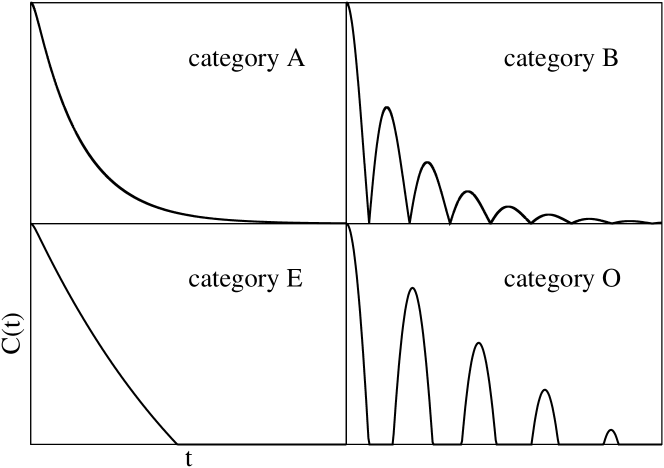
Figure 1: Four categories of entanglement evolution. $\mathcal{A}$: approaching. $\mathcal{B}$: bouncing. $\mathcal{E}$: entering. $\mathcal{O}$: oscillating. $\mathcal{A}$ and $\mathcal{B}$ belong to the HL class while $\mathcal{E}$ and $\mathcal{O}$ belong to the ESD class.

The existence of these categories can be explained by considering the trajectories $\vec{n}(t)$ and their relationships to $S$. Our basic premise is that three characteristics of any model determine the entanglement evolution categories: the dynamical subspace $D$ of the model, its limiting point $\vec{n}_{\infty}=\lim_{t\rightarrow\infty}\vec{n}(t)$ and the memory effect of the environment. $D$ is defined as the collection of possible trajectories in a model. It is necessary to introduce $D$ to understand how transitions between categories can happen. $D$ can be of lower dimension than $M$ if the evolution has any symmetries or if we limit the set of initial conditions in some way. The most important characterstic of any model is the set $D\cap S$. If $\dim D\cap S=\dim D$, all four categories are possible. On the other hand, if $\dim D\cap S<\dim D$, only $\mathcal{A}$- and $\mathcal{B}$-type behaviors are possible. This is because the measure of $T_{0}$ in $[0,\infty)$ can be no greater than the measure of $D\cap S$ in $D$.

The limiting state $\vec{n}_{\infty}$ exists for most physical decoherence processes; limit cycles and the like cannot be ruled out in general Terra_Cunha07 ; *Drumond09, but we will limit ourselves to the cases where $\vec{n}_{\infty}\in S$ and is unique. This constraint still leaves us with two possibilities: $\vec{n}_{\infty}\in\text{Int}(S)$ (the interior of $S$) and $\vec{n}_{\infty}\in B_{S}$. The first case guarantees the occurrence of categories $\mathcal{E}$ and $\mathcal{O}$ while the second one could give rise to all four possibilities depending on other details of $\vec{n}(t)$, for example, whether $\vec{n}_{\infty}$ is approached from $S$ or $M\setminus S$. We take as a working definition that Markovian trajectories satisfy the semigroup condition for all possible time partitioning Rivas10 ; *Breuer09; BreuerBook . Then Markovian evolutions are either in categories $\mathcal{A}$ or $\mathcal{E}$ while non-Markovian ones are typically in categories $\mathcal{B}$ and $\mathcal{O}$.

II.2 case study: a classical noise model

The aforementioned three characteristics of a model do not uniquely determine the category of entanglement evolution. Transitions between categories are thus possible by tuning some physical parameters of the model Yu04PRL . We now illustrate this with a general decoherence model that is nevertheless of low enough dimension that the topology can be visualized.

The two-qubit Hamiltonian for the model is

$$H=-\frac{1}{2}\sum_{K=A,B}\left[B_{K}Z_{K}+b_{K}\left(t\right)\vec{g}_{K}\cdot\vec{\sigma}_{K}\right],$$

where $\vec{\sigma}_{K}=(X_{K},Y_{K},Z_{K})$. The fields $b_{A,B}(t)$ are random time-dependent fields that decohere qubits A and B and they are not correlated in time. $B_{K}$ is a static field and $g_{K}$ is the noise coupling strength. For simplicity, we take $\vec{g}_{A}=\vec{g}_{B}=\vec{g}$. An important parameter in the model is $\theta$, defined by $\cos\theta=\hat{g}\cdot\hat{z}$. It is the angle between the energy axis and the noise axis. $\theta=0$ means that the noise is pure dephasing noise, while $\theta=\pi/2$ is transverse noise. If the correlation times of $b_{A,B}(t)$ are short (long) compared with $1/g\cos\theta$, the system is typically Markovian (non-Markovian) Zhou10PRA ; Galperin06 .

Decoherence in this classical noise model comes from the average over all noise histories $b_{K}(t)$. For more detailed discussions, see Ref. Joynt_2009 and also the section on Bloch-Wangsness-Redfield theory in Ref. Slichter96 .

We choose an initial state such that only $n_{XX}$, $n_{XY}$, $n_{YX}$, $n_{YY}$, and $n_{ZZ}$ are nonzero, and this condition is preserved in the subsequent motion. We further require $n_{XX}=n_{YY}$ and $n_{XY}=-n_{YX}$, which leaves only three independent parameters. This defines the dynamical subspace $D$ as a $3$-dimensional slice of $M$. We refer to this as $D_{3}$. $D_{3}$ is large enough to accommodate essentially any decoherence dynamics given that (1) the two qubits are non-interacting; (2) noises on the two qubits are uncorrelated in time; (3) the effect of dephasing and relaxation can be separated; (4) the initial state is in $D_{3}$. Thus $D_{3}$ is the dynamical manifold of a rather general class of decoherence processes. Note that $n_{XX}^{2}+n_{XY}^{2}=R^{2}$ is conserved in $D_{3}$. The positivity of the density matrix requires

$$a_{2}\geq 0 ~{}\Rightarrow~{}2R^{2}+n_{ZZ}^{2}\leq 3$$ (2)

$$a_{3}\geq 0 ~{}\Rightarrow~{}n_{ZZ}\leq 1-2R^{2},~{}\text{and}~{}n_{ZZ}\geq-1$$ (3)

$$a_{4}\geq 0 ~{}\Rightarrow~{}2R+n_{ZZ}\leq 1$$ (4)

where $a_{i}$ are the coefficients of the characteristic polynomial det$(xI\otimes I-\rho)=\sum_{j=0}^{N}(-1)^{j}a_{j}x^{N-j}$ Kimura03 .

Applying these inequalities, we find that $D_{3}$ is a cone in the ($n_{XX}$,$n_{XY}$,$n_{ZZ}$) coordinates. Its cross-section, as shown in Fig. 2, is an isosceles triangle with height $2$ and base $2$ and the full manifold is generated by rotation about the $n_{ZZ}$ axis. The concurrence is given by

$$C=\max\left\{0,R-(1+n_{ZZ})/{2}\right\}.$$ (5)

Separable states $S\cap D_{3}$ form a set with a spindle shape on top and the entangled states form a torus-like shape on the bottom with triangular cross sections. The direction of the gradient of $C$ is indicated by the filled arrows in Fig.2 and the maximally entangled Bell states $\left|\Psi\right\rangle=\frac{1}{2}\left(\left|01\right\rangle+e^{i\phi}\left|10\right\rangle\right)$ with $C=1$ form the circle $R=1$ and $n_{ZZ}=-1$ on the lower surface of the cone. It is tempting to consider the minimum Euclidean distance to separable states in the polarization vector representation as a geometric measure of entanglement Wei03 ; Cole10 . It indeed works in $D_{3}$ but whether it qualifies as an entanglement measure in general is still an open question Verstraete02 .

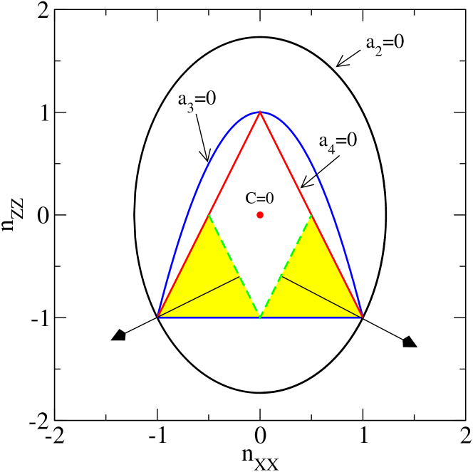
Figure 2: (Color online) Cross section of the dynamical subspace $D_{3}$ with $n_{XY}=0$. $a_{2}=0$ is the ellipse. $a_{3}=0$ gives the parabola and the bottom of the isosceles triangle. $a_{4}=0$ sets the two sides of the triangle. The entangled region is shaded where the filled arrows denote increasing direction of the concurrence. The green dashed line is the boundary of entangled and separable states, i.e., $B_{S}\cap D_{3}$. The fully mixed state is denoted by a red dot. This isosceles triangle corresponds to a projection of the tetrahedron in Ref. Horodecki96PRA .

We thus fully characterized the entanglement topology of $D_{3}$. Now we construct time evolutions in $D_{3}$. The initial state is taken as the generalized Werner state $\omega_{r}^{\Psi}=r\left|\Psi\right\rangle\left\langle\Psi\right|+\left(1-r\right)I_{4}/4$ Zhou10QIP ; Werner89 . Without any loss of generality, we choose $\phi=0$ in $|\Psi\rangle$, giving $n_{XY}=0$. This allows us to visualize the state and entanglement evolutions in a $2$-dimensional picture. The initial state is $\vec{n}(0)=(n_{XX},n_{ZZ})=(r,-r)$ and the state trajectory is given by

$$n_{XX}\left(t\right) =\left\langle X\otimes X\right\rangle(t)=r~{}\zeta^{AB}(t),$$ (6)

$$n_{ZZ}\left(t\right) =-r~{}e^{-\Gamma_{1}^{AB}t}.$$ (7)

where $\Gamma_{1}^{AB}=\Gamma_{1}^{A}+\Gamma_{1}^{B}$ is the overall longitudinal relaxation rate. $\zeta^{AB}=\zeta^{A}\zeta^{B}$ describes overall dephasing process. Note $\zeta\left(0\right)=1$ and $\zeta\left(\infty\right)=0$ if dephasing occurs. The details of $\zeta(t)$ and $\Gamma_{1}$ are model-dependent. For Markovian noises, the Bloch-Wangsness-Redfield theory applies and we have $\zeta^{K}(t)=\exp(-\Gamma_{2}^{K}t)$, where $\Gamma_{2}^{K}=\Gamma_{1}^{K}/2+\Gamma_{\phi}^{K}$, $\Gamma_{1}^{K}=g_{K}^{2}\sin^{2}\theta S^{K}(B_{k})/2$ and $\Gamma_{\phi}^{K}=g_{K}^{2}\cos^{2}\theta S^{K}(0)/2$ for $K=A,B$ Slichter96 . Here $S^{K}(\omega)$ is the power spectrum function (Fourier transform of the noise autocorrelation function) of the classical noise process $b_{K}(t)$. For non-Markovian noises, non-exponential behaviors in $\zeta(t)$, such as damped oscillations, are possible Zhou10QIP .

The direction of the trajectory in $D_{3}$ is determined by the relative weight of dephasing and relaxation noise on the qubits. The trajectories are characterized by two parameters, $r$ which fixes the initial position, and $\theta$, that weights the two types of noise. In the case of pure dephasing ($\theta=0$), $n_{ZZ}$ is constant and the trajectory is horizontal with $\vec{n}_{\infty}=(0,-r)$. This is a visualization of decoherence free subspace where the constants of the decoherence dynamics can be used to encode information Lidar98PRL ; *Bacon00. By contrast, when there is relaxation noise $(\theta\neq 0)$, the trajectory also moves vertically, so that when both types of noises are present, the trajectory will have $\vec{n}_{\infty}=\left(0,0\right)\in\text{Int}(S)$. Only one trajectory with $r=1$ and $\theta=0$ (pure dephasing), gives HL behavior since it remains in the entangled manifold except for $\vec{n}_{\infty}=(0,-1)\in B_{S}$. All other trajectories show ESD. We may summarize the situation in topological language by saying that HL behavior requires that $\vec{n}_{\infty}\in B_{S}$.

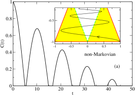
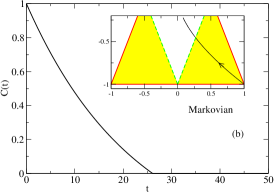
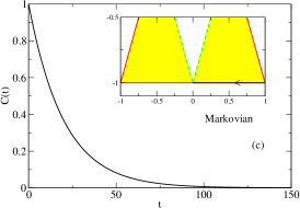
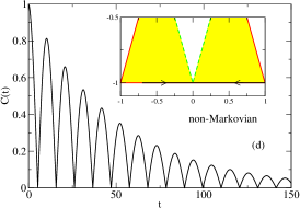
Figure 3: (Color online) Concurrence evolution and state trajectory (inset) in the presence of Markovian and non-Markovian noise. The arrows denote time direction. (a) and (b) have both dephasing and relaxation present, while (c) and (d) are the pure dephasing case. The initial state is Bell state $\left|\Psi+\right>$. We used $\zeta^{AB}=e^{-0.02t}\cos 0.3t$ for non-Markovian noise and $\zeta^{AB}=e^{-0.05t}$ for Markovian noise. For (a) and (b), $\Gamma_{1}^{AB}=0.03$.

To pin down the precise category of the entanglement evolution, we note that

$$C(t)=\max\left\{0,r\left[\zeta^{AB}\left(t\right)-\xi\left(t\right)\right]\right\}$$ (8)

where $\xi(t)=(1-re^{-\Gamma_{1}^{AB}t})/2$. If the noise is Markovian (non-Markovian) then $\zeta$ is monotonically decreasing (oscillatory) Bellomo08 ; Zhou10QIP ; Dajka08 ; Mazzola09 . In the latter case we find category $\mathcal{O}$, as the state trajectory enters and leaves the separable region as seen in Fig. 3a. In the case of Markovian noise, once the state leaves the entangled region, it leaves forever and we find category $\mathcal{E}$, as in Fig. 3b. There is a transition between this ESD behavior and HL behavior at the critical point $r=1$ and $\theta=0$. At this point we have $\vec{n}_{\infty}=(0,-1)\in B_{S}$. The transition is characterized by the fact that the “critical” trajectory intersects $B_{S}\cap D_{3}$ but not $\text{Int}(S)\cap D_{3}$. Markovian evolution yields category $\mathcal{A}$ behavior, as shown in Fig. 3c while non-Markovian behavior yields category $\mathcal{B}$ behavior as shown in Fig. 3d. Another perspective is that the dynamical subspace for these trajectories with $r=1$, $\theta=0$ is the bottom disc $D_{2}$ of $D_{3}$ and $\dim D_{2}\cap S=0<\dim D_{2}=2$. The transition of $T_{0}$ from the ESD class to HL class is thus a result of an topological transition of the dynamical subspace from $D_{3}$ to $D_{2}$.

III $N$-qubit case: GHZ and W states

Our examples have been drawn from the entanglement evolution of two-qubit systems. This is convenient, since the two-qubit concurrence is easily evaluated, and the lower dimensionality makes the examples relatively easy to visualize. However, it should be clear that the precise definition of entanglement is not important for the topological categorization. Only the definition of separability, which alone determines the set $S$, is crucial. As we saw above, the topological properties of $S$, particularly $\dim S=\dim M$, carry over to $N$-qubit systems. There are indications that as the dimension increases, the percentage of the separable states in the physical states decreases Zyczkowski98 ; Zyczkowski99 ; Gurvits03 ; *Gurvits05.

The entanglement measure for general multi-partite quantum system is a topic of current research Miyake03 ; *Osborne05; *Wong01; *deOliveira09; *Ou07; *Jung09; *Carvalho04; *Mintert05; Dur00 ; Vidal02 . The only easily computable entanglement measure for arbitrary $N$-qubit mixed states is the negativity Vidal02 , which measures the subsystem entanglement with respect to bipartite partitioning of the whole system. It is defined as

$$N(\rho)=\frac{\|\rho^{T_{A}}\|_{1}-1}{2}.$$ (9)

Here the norm is taken to be trace norm and $T_{A}$ denotes partial transpose on one of the two subsystems. $N(\rho)$ corresponds to the absolute value of the sum of the negative eigenvalues of $\rho^{T_{A}}$, which according to Peres-Horodeck’s criterion reveals the entanglement in $\rho$ Peres96 ; *Horodecki96Peres. Here we use $N(\rho)=0$ as a working criteria for separability.

We will use the negativity to illustrate the entanglement evolutions of $N$-qubit GHZ and W states due to pure dephasing noise. The GHZ state and W states are of interest to the quantum computing community since they possess different types of multi-partite entanglement and are used in various protocols such as quantum secret sharing, teleportation and super dense coding D'Hondt05 ; Dur00 ; Verstraete03 ; Tittel01 ; Yeo06 . The $N$-qubit GHZ and W states are defined to be

$$\left|{\text{GHZ}}\right>= \frac{\left|0\right>^{\otimes N}+\left|1\right>^{\otimes N}}{\sqrt{2}}$$ (10)

$$\left|{\text{W}}\right>= \frac{1}{\sqrt{N}}\left(\left|0\ldots 01\right>+\left|0\ldots 10\right>+\cdots+\left|1\ldots 00\right>\right).$$ (11)

The dephasing process on a single qubit can be described in terms of two Kraus operators Nielsen00Chuang ; Weinstein09jan

$$E_{0}=\begin{bmatrix}1&0\\ 0&\zeta(t)\end{bmatrix},\qquad E_{1}=\begin{bmatrix}0&0\\ 0&\sqrt{1-\zeta^{2}(t)}\end{bmatrix}.$$ (12)

Note $\zeta(t)$ is smooth and characterize the dephasing process in the $xy$ plane in the Bloch vector representation, just as in $D_{3}$. For simplicity, we assume that all qubits are independent and they share the same dephasing function $\zeta(t)$. Thus the full dynamics of the $N$-qubit system can be described by

$$\rho(t)=\sum_{i_{1},i_{2},\ldots,i_{N}}E_{i_{1}}E_{i_{2}}\cdots E_{i_{N}}\rho_{0}E_{i_{N}}^{\dagger}\cdots E_{i_{2}}^{\dagger}E_{i_{2}}^{\dagger}.$$ (13)

For the negativity, we make the $(1)(N-1)$ bipartite partition, i.e., the partial transpose is applied to one of the $N$ qubits. Due to the permutation symmetry of GHZ and W states, as well as the $N$-qubit Kraus operators, it does not matter which qubit is picked, indicating that the entanglement is evenly distributed among the $N$ qubits. Given these assumptions, the negativity of the $N$-qubit GHZ and W states are given by

$$N_{\text{GHZ}}= |\zeta|^{3}(t)/2$$ (14)

$$N_{\text{W}}= \frac{\sqrt{N-1}}{N}|\zeta|^{2}(t).$$ (15)

Notice that due to the smoothness of $\zeta(t)$, entanglement evolutions in categories $\mathcal{E}$ and $\mathcal{O}$ cannot happen. This can be explained by the topological argument as follows.

For both the GHZ and W states, the dephasing process does not expand the Hilbert space. For the $N$-qubit GHZ states, the density matrix can be expanded with identity and elements of the $su(2)$ algebra

$$\rho_{\text{GHZ}}=\frac{1}{2}\left(I+\sum_{i=X,Y,Z}n_{i}\sigma_{i}\right),$$ (16)

where $\sigma_{i}$ are defined on the two cat states, for example, $\sigma_{X}=|0\rangle^{\otimes N}\langle 1|^{\otimes N}+|1\rangle^{\otimes N}\langle 0|^{\otimes N}$. In other words, the dynamical subspace $D_{\text{GHZ}}$ for GHZ states under dephasing is a $3$-dimensional Bloch ball, as seen in Fig. 4. The negativity is given by

$$N(\rho_{\text{GHZ}})=\frac{n_{X}^{2}+n_{Y}^{2}}{2}.$$ (17)

The separable states in terms of negativity live on the vertical symmetry axis. We have

$$\dim D_{\text{GHZ}}\cap S=1<\dim D_{\text{GHZ}}=3$$

thus only entanglement evolutions in categories $\mathcal{A}$ and $\mathcal{B}$ are possible.

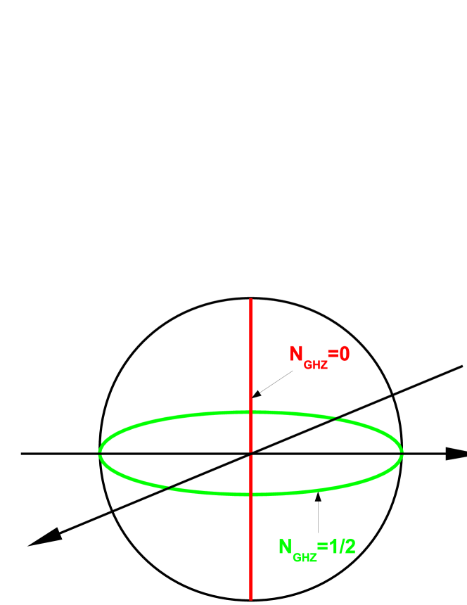
Figure 4: (Color online) Effective Bloch sphere representation for the dynmaical subspace $D_{\text{GHZ}}$ . The north and south pole are either $\left|0\right>^{N}$ or $\left|1\right>^{N}$. States resting on the red line connecting north and south pole have zero negativity. States on the green equator are maximally entangled.

For the W states, the density matrix is expanded with identity and elements of the $su(N)$ algebra. Thus the dynamical subspace $D_{\text{W}}$ is $N^{2}-1$ dimensional. However, when calculating negativity, the partial transpose introduces $N$ extra bases into the Hilbert space and $\rho^{T_{A}}(t)$ contains elements in $su(2N)$ algebra. The partial tranpose moves $N-1$ elements $\beta_{i}$ and their complex conjugates $\beta^{*}$ in the original density matrix to the blocks of the newly introduced bases. The positions of these elements $\beta_{i}$ are related to the partial transpose: suppose the partial transpose acts on the $k$’th qubit, then $\beta_{i}$ are the coefficients of $\left|\ldots 0\ldots\right>\left<\ldots 1\ldots\right|$, where $0$ and $1$ label the $k$’th qubit. Take the $3$-qubit case for example, the component $\beta_{1}|001\rangle\langle 100|$ is mapped into $\beta_{1}|101\rangle\langle 000|$, where the partial transpose is taken on the first (left-most) qubit. On the other hand, components such as $|001\rangle\langle 010|$ or $|100\rangle\langle 100|$ are left unchanged under the action of partial transpose on the first qubit.

The negativity for any density matrix expandable by the W state bases is given by

$$N(\rho_{{\text{W}}})=\frac{1}{N}\sqrt{\sum_{i=1}^{N-1}|\beta_{i}|^{2}}$$ (18)

Note that the condition of separability $N(\rho_{{\text{W}}})=0$ eliminates $2(N-1)$ degrees of freedom. Thus

$$\dim(D_{\text{W}}\cap S)=(N-1)^{2}<\dim D_{\text{W}}=N^{2}-1$$

and we conclude that entanglement evolutions in categories $\mathcal{E}$ and $\mathcal{O}$ are not possible.

IV summary

In summary, we found that there are four and only four types of natural behaviors for the time evolution of entanglement, given the initial state is entangled and the final one separable. These categories are determined by the dimensionality and intersection properties of sets in $M$. Since these properties are preserved by continuous deformations, they are topological. Three characteristics determine the categories: the dynamical subspace $D$ of the model, the limiting state $\vec{n}_{\infty}$ and the memory effect of the environment. Category $\mathcal{A}$ occurs (typically) for Markovian systems when $\vec{n}_{\infty}\in B_{S}$, category $\mathcal{B}$ occurs (typically) for non-Markovian systems when $\vec{n}_{\infty}\in B_{S}$. Category $\mathcal{E}$ occurs (typically) for Markovian systems, while category $\mathcal{O}$ occurs (typically) for non-Markovian systems. For those two categories, $\vec{n}_{\infty}$ can be either on the boundary or in the interior of $S$.

Model studies of entanglement evolution have shown a wide variety of behaviors, and a unifying picture of these behaviors has been lacking. The topological approach given here provides such a picture. The qualitative behavior is determined by relative dimensions of the dynamical subspace, the space of separable states, and the space formed by their intersection. The determination of these dimensions, together with the location of the asymptotic point, tells us when transitions between different types of evolution can be expected. Precise means of computing the dimensions, including the important role of symmetry, will be given in a future publication.

- (1) R. Horodecki, P. Horodecki, M. Horodecki, and K. Horodecki, Rev. Mod. Phys. 81, 865 (Jun 2009)
- (2) T. Yu and J. H. Eberly, Science 323, 598 (2009)
- (3) K. Zyczkowski, P. Horodecki, M. Horodecki, and R. Horodecki, Phys. Rev. A 65, 012101 (Dec 2001)
- (4) T. Yu and J. H. Eberly, Phys. Rev. Lett. 93, 140404 (Sep 2004)
- (5) T. Yu and J. H. Eberly, Phys. Rev. Lett. 97, 140403 (Oct 2006)
- (6) T. Yu and J. Eberly, Optics Communications 283, 676 (2010)
- (7) T. Yu and J. Eberly, Optics Communications 264, 393 (2006)
- (8) B. Bellomo, R. Lo Franco, and G. Compagno, Phys. Rev. Lett. 99, 160502 (Oct 2007)
- (9) B. Bellomo, R. Lo Franco, and G. Compagno, Phys. Rev. A 77, 032342 (Mar 2008)
- (10) J. Dajka, M. Mierzejewski, and J. Luczka, Phys. Rev. A 77, 042316 (Apr 2008)
- (11) M. J. Testolin, J. H. Cole, and L. C. L. Hollenberg, Phys. Rev. A 80, 042326 (Oct 2009)
- (12) D. Braun, Phys. Rev. Lett. 89, 277901 (Dec 2002)
- (13) Z. Ficek and R. Tanaś, Phys. Rev. A 74, 024304 (Aug 2006)
- (14) L. Mazzola, S. Maniscalco, J. Piilo, K.-A. Suominen, and B. M. Garraway, Phys. Rev. A 79, 042302 (Apr 2009)
- (15) D. Zhou, A. Lang, and R. Joynt, Quant. Info. Processing 9, 727 (March 2010)
- (16) J. H. Cole, Journal of Physics A: Mathematical and Theoretical 43, 135301 (2010)
- (17) C. E. A. Jarvis, D. A. Rodrigues, B. L. Györffy, T. P. Spiller, A. J. Short, and J. F. Annett, New Journal of Physics 11, 103047 (2009)
- (18) A. De, A. Lang, D. Zhou, and R. Joynt, Phys. Rev. A 83, 042331 (Apr 2011)
- (19) M. P. Almeida, F. de Melo, M. Hor-Meyll, A. Salles, S. P. Walborn, P. H. S. Ribeiro, and L. Davidovich, Science 316, 579 (2007)
- (20) J. Laurat, K. S. Choi, H. Deng, C. W. Chou, and H. J. Kimble, Phys. Rev. Lett. 99, 180504 (Nov 2007)
- (21) J.-S. Xu, C.-F. Li, M. Gong, X.-B. Zou, C.-H. Shi, G. Chen, and G.-C. Guo, Phys. Rev. Lett. 104, 100502 (Mar 2010)
- (22) G. Kimura, Physics Letters A 314, 339 (2003)
- (23) M. S. Byrd and N. Khaneja, Phys. Rev. A 68, 062322 (Dec 2003)
- (24) G. Mahler and R. Wawer, Quantum Networks: Dynamics of Open Nanostructures, 2nd ed. (Springer, 1998)
- (25) R. Alicki and K. Lendi, Quantum dynamical semigroups and applications (Springer-Verlag, 1987)
- (26) R. Joynt, D. Zhou, and Q.-H. Wang, Int. J. Mod. B 25, 2115 (2011)
- (27) J. M. Chow, L. DiCarlo, J. M. Gambetta, A. Nunnenkamp, L. S. Bishop, L. Frunzio, M. H. Devoret, S. M. Girvin, and R. J. Schoelkopf, Phys. Rev. A 81, 062325 (Jun 2010)
- (28) L. DiCarlo, M. Reed, L. Sun, B. Johnson, J. Chow, J. Gambetta, L. Frunzio, S. Girvin, M. Devoret, and R. Schoelkopf, Nature 467, 574 (2010)
- (29) W. K. Wootters, Phys. Rev. Lett. 80, 2245 (Mar 1998)
- (30) K. Zyczkowski, P. Horodecki, A. Sanpera, and M. Lewenstein, Phys. Rev. A 58, 883 (Aug 1998)
- (31) M. O. Terra Cunha, New Journal of Physics 9, 237 (2007)
- (32) R. C. Drumond and M. O. T. Cunha, J. of Phys. A 42, 285308 (2009)
- (33) A. Rivas, S. F. Huelga, and M. B. Plenio, Phys. Rev. Lett. 105, 050403 (Jul 2010)
- (34) H.-P. Breuer, E.-M. Laine, and J. Piilo, Phys. Rev. Lett. 103, 210401 (Nov 2009)
- (35) H.-P. Breuer and F. Petruccione, The theory of open quantum systems (Oxford University Press, USA, 2007)
- (36) D. Zhou and R. Joynt, Phys. Rev. A 81, 010103 (Jan 2010)
- (37) Y. M. Galperin, B. L. Altshuler, J. Bergli, and D. V. Shantsev, Phys. Rev. Lett. 96, 097009 (Mar 2006)
- (38) C. P. Slichter, Principles of Magnetic Resonance, third edition ed. (Springer, New York, 1996)
- (39) T.-C. Wei and P. M. Goldbart, Phys. Rev. A 68, 042307 (Oct 2003)
- (40) F. Verstraete, J. Dehaene, and B. D. Moor, J. Mod. Opt. 49, 1277 (2002)
- (41) R. Horodecki and M. Horodecki, Phys. Rev. A 54, 1838 (Sep 1996)
- (42) R. F. Werner, Phys. Rev. A 40, 4277 (Oct 1989)
- (43) D. A. Lidar, I. L. Chuang, and K. B. Whaley, Phys. Rev. Lett. 81, 2594 (Sep 1998)
- (44) D. Bacon, J. Kempe, D. A. Lidar, and K. B. Whaley, Phys. Rev. Lett. 85, 1758 (Aug 2000)
- (45) K. Zyczkowski, Phys. Rev. A 60, 3496 (Nov 1999)
- (46) L. Gurvits and H. Barnum, Phys. Rev. A 68, 042312 (Oct 2003)
- (47) L. Gurvits and H. Barnum, Phys. Rev. A 72, 032322 (Sep 2005)
- (48) A. Miyake, Phys. Rev. A 67, 012108 (Jan 2003)
- (49) T. J. Osborne, Phys. Rev. A 72, 022309 (Aug 2005)
- (50) A. Wong and N. Christensen, Phys. Rev. A 63, 044301 (Mar 2001)
- (51) T. R. de Oliveira, Phys. Rev. A 80, 022331 (Aug 2009)
- (52) Y.-C. Ou and H. Fan, Phys. Rev. A 75, 062308 (Jun 2007)
- (53) E. Jung, M.-R. Hwang, D. Park, and J.-W. Son, Phys. Rev. A 79, 024306 (Feb 2009)
- (54) A. R. R. Carvalho, F. Mintert, and A. Buchleitner, Phys. Rev. Lett. 93, 230501 (Dec 2004)
- (55) F. Mintert, M. Kuś, and A. Buchleitner, Phys. Rev. Lett. 95, 260502 (Dec 2005)
- (56) W. Dür, G. Vidal, and J. I. Cirac, Phys. Rev. A 62, 062314 (Nov 2000)
- (57) G. Vidal and R. F. Werner, Phys. Rev. A 65, 032314 (Feb 2002)
- (58) A. Peres, Phys. Rev. Lett. 77, 1413 (Aug 1996)
- (59) M. Horodecki, P. Horodecki, and R. Horodecki, Phys. Lett. A 223, 1 (1996)
- (60) E. D’Hondt and P. Panangaden, Quant. Inf. Comput. 6, 173 (2005)
- (61) F. Verstraete, J. Dehaene, and B. De Moor, Phys. Rev. A 68, 012103 (Jul 2003)
- (62) W. Tittel, H. Zbinden, and N. Gisin, Phys. Rev. A 63, 042301 (Mar 2001)
- (63) Y. Yeo and W. K. Chua, Phys. Rev. Lett. 96, 060502 (Feb 2006)
- (64) M. A. Nielsen and I. L. Chuang, Quantum Computation and Quantum Information, 1st ed. (Cambridge University Press, 2000)
- (65) Y. S. Weinstein, Phys. Rev. A 79, 012318 (Jan 2009)