Vus and neutron beta decay

Abstract

We discuss the effect of the recent change of $V_{\rm us}$ by three standard deviations on the standard model predictions for neutron beta decay observables. We also discuss the effect the experimental error bars of $V_{\rm us}$ have on such predictions. Refined precision tests of the standard model will be made by a combined effort to improve measurements in neutron beta decay and in strangeness-changing decays. By itself the former will yield very precise measurements of $V_{\rm ud}$ and make also very precise predictions for $V_{\rm us}$.

I Introduction

The precision measurements of the decay rate R and the electron-asymmetry $\alpha_{e}$ in neutron beta decay (n$\beta$d) pdg06 and their further improvements in a near future provide an excellent opportunity to test the standard model (SM) review and even to establish deviations signaling new physics. However, the predictions for these observables are afflicted by our current inability to compute reliably the Cabibbo-Kobayashi-Maskawa (CKM) matrix element $V_{\rm ud}$ and the leading form factor ratio $\lambda=g_{1}/f_{1}$. Both are better handled as free parameters to be determined from experiment. The theoretical predictions are then confined to a region in the $(\alpha_{e},R)$ plane or equivalently in the $(\lambda,R)$ plane where the SM is expected to remain valid within a certain confidence level (CL), say $90\%$. This region may be referred to as the standard model region (SMR). At first, it may look as if the predictions of SM are severely limited by the experimental situation of $R$ and $\alpha_{e}$. However, this is not the case.

In a previous paper garcia02 we showed that the SMR is determined by the validity of the formulas predicted by the SM for the observables in n$\beta$d and of the CKM unitarity. The size of the SMR depends on the theoretical uncertainties of such formulas and the experimental values of $V_{\rm us}$ and $V_{\rm ub}$. Since such uncertainties in $R$ and $\alpha_{e}$ are substantially smaller than their experimental error bars, a much more narrow SMR can be predicted even when $V_{\rm ud}$ and $\lambda$ remain as free parameters. The predictions of SM are then greatly improved and it is these ones that are meaningful to compare with the measured $R$ and $\alpha_{e}$.

Nevertheless, such predictions are indeed affected by the experimental values of $V_{\rm ub}$ and $V_{\rm us}$. The former is quite precise already and its changes do not produce perceptible changes in the SMR. However, changes in $V_{\rm us}$ do produce important changes in the position and size of the SMR. It is the purpose of this paper to extend the analysis of Ref. garcia02 and discuss the dependence of the SMR on the value of $V_{\rm us}$. This has become more pressing since recently pdg06 its experimental value increased by three standard deviations from the value available for the analysis of garcia02 .

In Sec. II we shall review the SM formulas for n$\beta$d observables and the method to determine the predicted SMR. In Sec. III we shall determine the changes in the SMR corresponding to the new value of $V_{\rm us}$. We shall also determine its position allowing for variations of up to three standard deviations of the present $V_{\rm us}$. The role of $V_{\rm us}$ has another aspect, its precision affects importantly the size of the SMR. This will be studied in Sec. IV. A complementary analysis comes from the fact that precise measurements of $R$ and $\alpha_{e}$ will produce a precise determination of $V_{\rm ud}$. Assuming the validity of the unitarity of the CKM matrix, then n$\beta$d can make quite precise predictions for $V_{\rm us}$. We shall go into them in Sec. V. The last section is reserved for discussions and conclusions.

II Determination of the standard model region

The SM predicts for the decay rate of n$\beta$d the expression

$$R(10^{-3}\,{\rm s}^{-1})=|V_{\rm ud}|^{2}(0.1897)(1+3\lambda^{2})(1+0.0739\pm 0.0008)$$ (1)

at the level of a precision of $10^{-4}$. $V_{\rm ud}$ and $\lambda$ appear as free parameters. The detailed derivation of Eq. (1) is found in Ref. garcia01 . The main source of uncertainty in (1) is the model dependence of the contributions of $Z^{0}$ to the radiative corrections. A very conservative estimate is $\pm 0.0008$ marciano86 . If one assumes dominance of the $A_{1}$ resonance wilkinson94 this uncertainty becomes the uncertainty of such an approximation and then in Eq. (1) it can be estimated to be somewhat less than $\pm 0.0002$. Other uncertainties as in the values of the induced weak magnetism and pseudo-tensor form factors can be shown to contribute to $10^{-5}$ or less. Eq. (1) has also been discussed in Ref. czarnecki04 , where it was referred to as the master formula. Although presented in a somewhat different form, one can readily verify that the result of this reference confirms Eq. (1).

At the $10^{-4}$ level the SM predicts for the electron-asymmetry the expression garcialuna06

$$\alpha_{e}=\frac{-0.2089\times 10^{-3}+0.2763\lambda-0.2772\lambda^{2}}{0.1897+0.5692\lambda^{2}}.$$ (2)

We have chosen a negative sign for $\lambda$ to conform with the convention of pdg06 . The important remark here is that there is no theoretical uncertainty in $\alpha_{e}$ at this level of precision. The reason for this is that the uncertainty introduced by $Z^{0}$ is common to the numerator and denominator of $\alpha_{e}$ and cancels away at the $10^{-4}$ level. It must be stressed that $\alpha_{e}$ depends only on $\lambda$, so that the experimental determination of $\lambda$ is independent of $V_{\rm ud}$.

The analysis that leads to Eq. (2) can be extended to the neutrino and electron-neutrino asymmetry coefficients. We shall not go further into this because it has remained customary to present experimental results for the old order zero angular coefficients pdg06 ,

$$B_{0}=\frac{2\lambda(\lambda-1)}{1+3\lambda^{2}},$$ (3)

$$a_{0}=\frac{1-\lambda^{2}}{1+3\lambda^{2}}.$$ (4)

Also, instead of presenting results for $\alpha_{e}$ it is customary to give directly the value for $\lambda$, after all corrections contained in $\alpha_{e}$ have been applied to the experimental analysis. Thus, the relevance of exhibiting Eq. (2) is to show that the experimental value of $\lambda$ is free of theoretical uncertainties at the $10^{-4}$ level.

Another very important constraint for our work here is the unitarity of the CKM matrix, which we shall use in the form

$$V_{\rm ub}=\sqrt{1-V^{2}_{\rm ud}-V^{2}_{\rm us}}.$$ (5)

Given the experimental values of $V_{\rm ub}$ and $V_{\rm us}$, the only free parameter in Eq. (5) is $V_{\rm ud}$.

The current experimental situation pdg06 for Eqs. (1), (3), (4), and (5) is given by $R=1.12905(102)\times 10^{-3}\,{\rm s}^{-1}$, $B_{0}=0.981(4)$, $a_{0}=-0.103(4)$, $V_{\rm ub}=0.00431(30)$, and $V_{\rm us}=0.2257(21)$. It is this last number that recently increased by three standard deviations from its previous value and whose effect on the SMR we are going to determine. The experimental situation of $\lambda$ is at present ambiguous. Its four more precise determinations are $\lambda_{\rm A}=-1.2739(19)$ abele02 , $\lambda_{\rm L}=-1.266(4)$ liaud97 , $\lambda_{\rm Y}=-1.2594(38)$ yerozolimsky97 , and $\lambda_{\rm B}=-1.262(5)$ bopp86 . The last three are statistically compatible and produce an average $\lambda_{\rm LYB}=-1.2624(24)$. This average is not statistically compatible with the value $\lambda_{\rm A}$. Although one may quote an average of the four $\lambda_{\rm ALYB}=-1.2695(15)$, one must remember that such an average is not a consistent one. Even so, it will still be interesting to discuss it.

To determine the SMR we shall form a $\chi^{2}$ function with the six constraints Eqs. (1), (3), (4), (5), $V^{\rm exp}_{\rm ub}$, and $V^{\rm exp}_{\rm us}$. This is an over constrained system of restrictions for three free parameters $\lambda$, $V_{\rm ud}$, and $V_{\rm us}$. This function is

$$\chi^{2} = \left(\frac{R^{\prime}-R}{\sigma_{R^{\prime}}}\right)^{2}+\left(\frac{\lambda^{\prime}-\lambda}{\sigma_{\lambda^{\prime}}}\right)^{2}+\left(\frac{B^{\rm exp}_{0}-B_{0}}{\sigma_{B_{0}}}\right)^{2}+\left(\frac{a^{\rm exp}_{0}-a_{0}}{\sigma_{a_{0}}}\right)^{2}+$$ (6)

$$+\left(\frac{V^{\rm exp}_{\rm ub}-V_{\rm ub}}{\sigma_{V_{\rm ub}}}\right)^{2}+\left(\frac{V^{\rm exp}_{\rm us}-V_{\rm us}}{\sigma_{V_{\rm us}}}\right)^{2}.$$

The SMR is determined by minimizing ${\chi}^{2}$ at a fine lattice of points ($\lambda^{\prime}$, $R^{\prime}$) in the ($\lambda$, $R$) plane. It will correspond to the $90\%$ CL region in this plane. That is, within this region the SM may be expected to remain valid at the $90\%$ CL.

The key element in the determination of the SMR is that $\sigma_{R^{\prime}}$ and $\sigma_{\lambda^{\prime}}$ are not limited to take their current experimental values $\sigma_{R}=0.00102\times 10^{-3}\,{\rm s}^{-1}$ and $\sigma_{\lambda}$ around 0.0024. We are at liberty to reduce them down to their theoretical uncertainty, namely, a few parts at $10^{-4}$. The theoretically predicted SMR will correspond to $\sigma_{R^{\prime}}$ and $\sigma_{\lambda^{\prime}}$ at approximately one-tenth of their current experimental counterparts.

In the next two sections we shall study the effects of $V_{\rm us}$ on the determination of the SMR. Its central value will affect its position in the ($\lambda$, $R$) plane and its error bar will affect its width.

III $\bm{V_{\rm us}}$ and the standard model region

We shall work within a rectangle of the ($\lambda$, $R$) plane. The side for $\lambda$ will be $(-1.2744,-1.2552)$ due to the ambiguity of the experimental value of $\lambda$ range . We shall fold by quadratures the theoretical uncertainty of $R$ into its experimental error bar to get an effective $\sigma_{R}=0.00132\times 10^{-3}\,{\rm s}^{-1}$. The other side of the rectangle will cover three effective standard deviations above and below the central value of $R=1.12905\times 10^{-3}\,{\rm s}^{-1}$.

To study the effect of $V_{\rm us}$ upon the SMR we shall let its central value vary up to three standard deviations $\sigma_{V_{\rm us}}=0.0021$ above and below its current central value $V_{\rm us}=0.2257$. The other three restrictions in (6) will be kept fixed at their current experimental values.

There is no need to present all the details of our numerical analysis. Our results are well illustrated by exhibiting three cases for the central value of $V_{\rm us}$, namely, 0.2194, 0.2257, and 0.2320 (the first one corresponds to the previous value of $V_{\rm us}$, the second one to its current value, and the third one allows for still another three-sigma increase of $V_{\rm us}$). In each of these cases we use the liberty we have to choose the size of $\sigma_{R^{\prime}}$ and $\sigma_{\lambda^{\prime}}$. The first choice for them is the corresponding experimental error bars 0.00132 and 0.0024. The resulting SMR could well be referred to as the “experimental” SMR. The second choice is to use one-tenth of these values, which as discussed in the last section is the theoretical SMR. And for the purpose of further discussion we use as a third choice one-hundredth of such values.

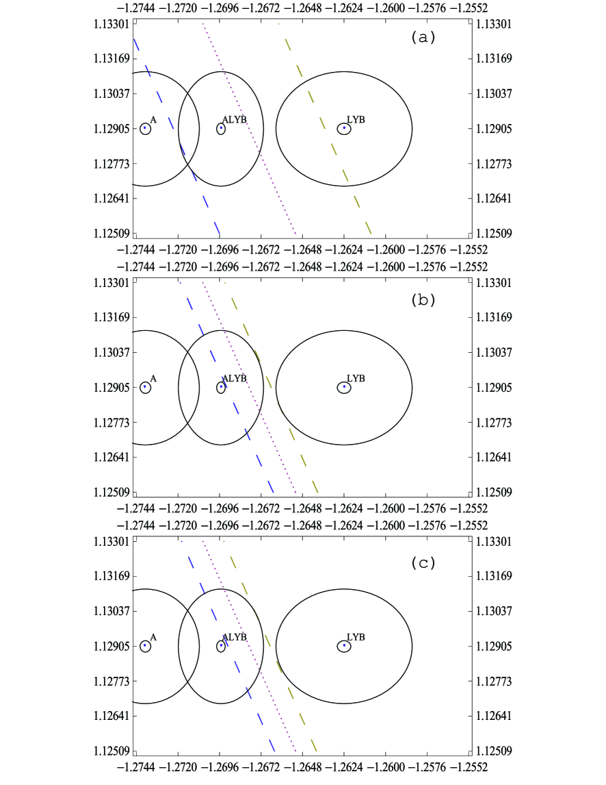
Figure 1: The detailed numerical results corresponding to Table 1 are plotted here. The upper, middle, and lower entries correspond to (a), (b), and (c), respectively.

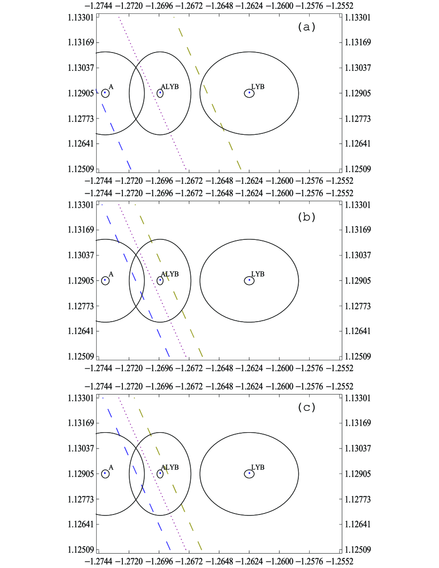
Figure 2: The detailed numerical results corresponding to Table 2 are plotted here. The upper, middle, and lower entries correspond to (a), (b), and (c), respectively.

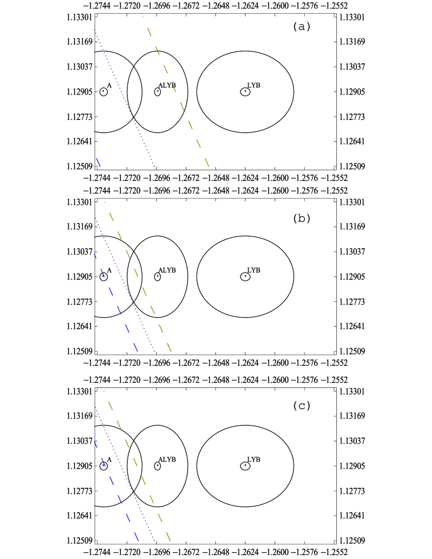
Figure 3: The detailed numerical results corresponding to Table 3 are plotted here. The upper, middle, and lower entries correspond to (a), (b), and (c), respectively.

Our numerical results are given in Tables 1, 2, and 3. The rows correspond to steps of one standard deviation in $R^{\prime}$, $\lambda_{0}$ gives the corresponding position of the minimum $\chi^{2}_{0}$, the $90\%$ CL ranges of $\lambda^{\prime}$ are given in the column headed by $\lambda^{\prime}$. In each case the SMR is a band. This can be visualized in the corresponding Figures 1, 2, and 3.

To appreciate the variation of $\chi^{2}$ within the rectangle in the ($\lambda$, $R$) plane we list its value at sample points in Tables 4, 5, and 6. In these tables one can see how the SMR is narrowed as $\sigma_{R^{\prime}}$ and $\sigma_{\lambda^{\prime}}$ are reduced from their experimental values to one-tenth of them. But, one also sees that reducing them further produces no significant narrowing any more.

For comparison purposes, we include in Figures 1, 2, and 3 the $90\%$ CL region around the central values of the current measurements and, also, the same regions at one-tenth of the present error bars. Although the effect of changing $V_{\rm us}$ is perceptible for the “experimental” SMR in Figs. 1 (a), 2 (a), and 3 (a) it does not lead to sharp conclusions, unless $V_{\rm us}$ were to reach $0.2320$. In contrast, the theoretical SMR of Figs. 1 (b), 2 (b), and 3 (b) clearly discriminate $\lambda_{\rm A}$ and $\lambda_{\rm LYB}$. The current situation is depicted in Fig. 2 (b). $\lambda_{\rm LYB}$ is sharply incompatible with the SM. Thus, either the SM is quite accurate and $\lambda_{\rm LYB}$ will be eliminated or, if this $\lambda_{\rm LYB}$ is confirmed in the future, n$\beta$d will produce strong evidence for not too far away new physics. Correspondingly, if $\lambda_{\rm A}$ is confirmed in the future, the accuracy of the SM will be sustained and new physics will be farther away; so it will be harder to detect it in n$\beta$d. The above disjunctive is further strengthened if $V_{\rm us}$ is measured still higher, as seen in Fig. 3 (b). Notice that the current central values of $\lambda_{\rm A}$ and $\lambda_{\rm LYB}$, if either of them were to be confirmed, strongly indicate the existence of new physics, as can be appreciated with the small regions around them in Fig. 2 (b). The SM would remain very accurate if $\lambda_{\rm A}$ were confirmed and $V_{\rm us}$ were further increased up to $0.2320$. This possibility is illustrated in Fig. 3 (c). Surprisingly, the inconsistent average $\lambda_{\rm ALYB}$ is fully compatible with the SM at present, as seen in Fig. 2 (b).

That arbitrarily reducing $\sigma_{R^{\prime}}$ and $\sigma_{\lambda^{\prime}}$ up to one-hundredth of their experimental counterparts produced no significant reduction of the SMR, as can be seen in Figs. 1 (c), 2 (c), and 3 (c), requires some detailed discussion. The reason for this can be traced to the individual contributions of $R^{\prime}$, $\lambda^{\prime}$, and $V_{\rm us}$ to $\chi^{2}$ of Eq. (6). In this respect, we have produced Table 7. It is sufficient to present the case of the central row in Table 2, where $V_{\rm us}=V^{\rm exp}_{\rm us}=0.2257$ and $R=R^{\rm exp}=1.12905\times 10^{-3}\,{\rm s}^{-1}$, and the contributions to $\chi^{2}$ at the border of the SMR, namely, the extremes of the corresponding ranges of $\lambda^{\prime}$ in Table 2.

In the top part of Table 7 we give the six different contributions to $\chi^{2}$ at the above extremes. One can see that with $\sigma_{R^{\prime}}$ and $\sigma_{\lambda^{\prime}}$ at their experimental values the $\chi^{2}(R^{\prime})$ and $\chi^{2}(\lambda^{\prime})$ contributions dominate over the $\chi^{2}(V_{\rm us})$ contribution (upper entries). At $1/10$ of these values the situation is reversed and it remains so when $\sigma_{R^{\prime}}$ and $\sigma_{\lambda^{\prime}}$ are reduced up to $1/100$ (second and third entries). In the lower part of Table 7 we trace in more detail when this reversal takes place by reducing $\sigma_{R^{\prime}}$ and $\sigma_{\lambda^{\prime}}$ by $1/2$, $1/5$, and $1/7$ (second, third, and fourth entries, respectively). The dominance of $\chi^{2}(V_{\rm us})$ over $\chi^{2}(R^{\prime})$ and $\chi^{2}(\lambda^{\prime})$ takes place already when $\sigma_{R^{\prime}}$ and $\sigma_{\lambda^{\prime}}$ are cut to between $1/4$ and $1/5$ of their experimental counterparts. Notice that this reversal does not depend on $B_{0}$, $a_{0}$, and $V_{\rm ub}$, whose $\chi^{2}$ contributions remain fairly constant throughout Table 7. One may conclude that the potential of the SM prediction at $1/10$ of the experimental errors on $R$ and $\lambda$ cannot be reached, because of the current uncertainty on $V_{\rm us}$. In other words, even if the experimental precision in n$\beta$d were to be greatly improved in the near future, the comparison with the SM predictions will be severely limited by the experimental precision of $V_{\rm us}$.

Let us next study in detail the effects of improving the precision of $V_{\rm us}$.

IV The precision of $\bm{V_{\rm us}}$ and the standard model region

n$\beta$d cannot provide a better test of the SM even if the error bars on $R$ and $\lambda$ and the theoretical uncertainty in Eq. (1) were to be reduced beyond one-fifth. As seen in the previous section, the limitation comes from the error bars on $V_{\rm us}$. The central value of $V_{\rm us}$ does shift the position of the SMR, but it is reducing $\sigma_{V_{\rm us}}$ that will improve the width of the SMR.

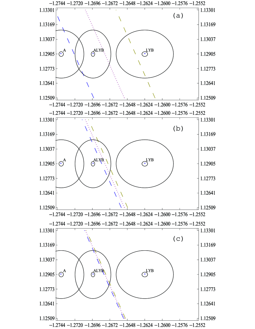
Figure 4: These figures correspond to Figs. 1 (a), 1 (b), and 1 (c) when $\sigma_{V_{\rm us}}$ is assumed to be at $0.00021$.

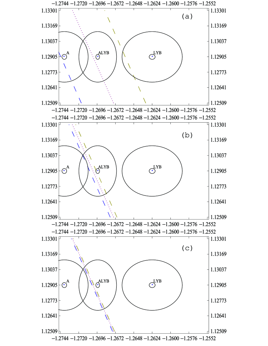
Figure 5: These figures correspond to Figs. 2 (a), 2 (b), and 2 (c) when $\sigma_{V_{\rm us}}$ is assumed to be at $0.00021$.

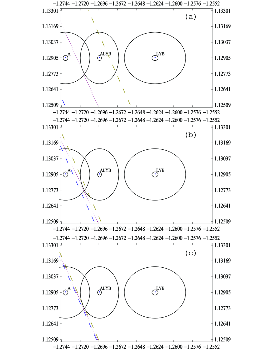
Figure 6: These figures correspond to Figs. 3 (a), 3 (b), and 3 (c) when $\sigma_{V_{\rm us}}$ is assumed to be at $0.00021$.

To see this we have reproduced the SMR assuming $\sigma_{V_{\rm us}}$ is cut to one-tenth of its current value, that is $\sigma_{V_{\rm us}}=0.00021$, and assuming the central value to be at three places, $V_{\rm us}=0.2194$, 0.2257, or 0.2320. Of course this last is only an assumption, all we can say as of now is that such central value will fall at $90\%$ CL somewhere within the band of Fig. 2 (b). The corresponding numerical results are summarized in Tables 8, 9, and 10 for $\chi^{2}_{0}$, $\lambda_{0}$, and the $90\%$ CL range of $\lambda^{\prime}$. Values of $\chi^{2}$ at sample points in the ($\lambda$, $R$) plane are found in Tables 11, 12, and 13. In each row of these six tables the upper, middle, and lower entries correspond to $\sigma_{R^{\prime}}$ and $\sigma_{\lambda^{\prime}}$ at $\sigma_{R}$ and $\sigma_{\lambda}$, at $\sigma_{R}/10$ and $\sigma_{\lambda}/10$, and at $\sigma_{R}/100$ and $\sigma_{\lambda}/100$, respectively. Notice that the numerical values of $\chi^{2}_{0}$ and $\lambda_{0}$ are practically the same in Tables 1 and 8, 2 and 9, and 3 and 10. The minimum of $\chi^{2}$ and the position of the minimum in the ($\lambda$, $R$) plane are practically independent of the values of $\sigma_{R^{\prime}}$, $\sigma_{\lambda^{\prime}}$, and $\sigma_{V_{\rm us}}$. In contrast, the values of $\chi^{2}$ at sample points in the ($\lambda$, $R$) plane away from the SMR become enormous, as can be appreciated looking throughout Tables 11, 12, and 13. Such increases in $\chi^{2}$ indicate the substantial narrowing of the SMR as $\sigma_{V_{\rm us}}$ is reduced along with $\sigma_{R^{\prime}}$ and $\sigma_{\lambda^{\prime}}$. These results can be visualized in Figs. 4, 5, and 6. Comparing these last figures with the corresponding ones of Sec. III, one sees that the “experimental” SMR is not noticeably reduced, as was to be expected. However, at one-tenth $\sigma_{R^{\prime}}$ and $\sigma_{\lambda^{\prime}}$, the comparison of Figs. 1 (b), 2 (b), and 3 (b), with Figs. 4 (b), 5 (b), and 6 (b), respectively, shows that the effect of reducing $\sigma_{V_{\rm us}}$ is quite impressive. As seen in Tables 11, 12, and 13, the SMR is greatly reduced. This reduction of the SMR could lead to almost a thin line if the theoretical and experimental uncertainties in $R$ and $\lambda$ were put under much better control, as can be visualized in Figs. 4 (c), 5 (c), and 6 (c).

There is a systematic feature in Tables 1-3 and Tables 8-10, the value of $\chi^{2}_{0}$ is always around $2.90$. The reason for this is found in Table 7, the contribution of the neutrino asymmetry $B_{0}$ to $\chi^{2}$ is always around $2.70$. This is a $1.6$ standard deviations from the SM prediction. It is not significant and we shall not discuss it further.

It is clear that the ability of n$\beta$d to test the SM is intimately connected with the precision to determine $V_{\rm us}$ in strangeness-changing decays.

V Predictions of $\bm{V_{\rm us}}$ from neutron beta decay

A precise determination of $V_{\rm us}$ in strangeness-changing decays may take longer than precise measurements of $R$ and $\alpha_{e}$ or $\lambda$. n$\beta$d may provide a better determination of $V_{\rm us}$ via the unitarity of the CKM matrix, once the former produce a precise measurement of $V_{\rm ud}$. This is a complementary way to appreciate the results of the last two sections.

First, let us look into the current determination of $V_{\rm ud}$. The ambiguity in $\lambda$ leads to an ambiguity in the experimental value of $V_{\rm ud}$. One has correspondingly two incompatible values for $V_{\rm ud}$, namely,

$$V^{\rm LYB}_{\rm ud}=0.9791\pm 0.0016$$ (7)

and

$$V^{\rm A}_{\rm ud}=0.9718\pm 0.0013.$$ (8)

One may also quote the third, albeit inconsistent, value

$$V^{\rm ALYB}_{\rm ud}=0.9746\pm 0.0011.$$ (9)

Although, not yet satisfactory, one can already see that the error bars are competitive with $V_{\rm ud}$ determined from other sources pdg06 . Also, within the validity of the SM, these values are accompanied by

$$V^{\rm LYB}_{\rm us}=0.2032\pm 0.0079,$$ (10)

$$V^{\rm A}_{\rm us}=0.2357\pm 0.0055,$$ (11)

and

$$V^{\rm ALYB}_{\rm us}=0.2239\pm 0.0048.$$ (12)

Again, even if not satisfactory, the error bars are becoming competitive with $V_{\rm us}$ determined from other sources pdg06 .

Let us match Eqs. (10)-(12) with the value of $V_{\rm us}$ from $K_{l3}$ decays (which was used in the previous sections), namely,

$$V^{K_{l3}}_{\rm us}=0.2257\pm 0.0021.$$ (13)

It is convenient to produce the $90\%$ CL ranges that correspond to these $V_{\rm us}$ values. They are

$$V^{\rm LYB}_{\rm us}(90\%\,{\rm CL})=(0.1905,\,0.2159),$$ (14)

$$V^{\rm A}_{\rm us}(90\%\,{\rm CL})=(0.2270,\,0.2444),$$ (15)

$$V^{\rm ALYB}_{\rm us}(90\%\,{\rm CL})=(0.2163,\,0.2315),$$ (16)

and

$$V^{K_{l3}}_{\rm us}(90\%\,{\rm CL})=(0.2222,\,0.2292).$$ (17)

One can readily see that range (14) is below (17) and there is no overlap between them at all. Range (15) is above (17) and there is a small overlap between the two. Contrastingly, range (16) fully contains range (17). These comparisons correspond to the overlapping or lack of it of the $90\%$ CL ellipses with the SMR exhibited in Fig. 2 (b).

Also, they indirectly exhibit the current experimental problem in the determination of $\lambda$. Ranges (14) and (15) do not overlap with one another and are quite separated. These comparisons are complementary to the analysis of sections III and IV. They provide a quick way to see the compatibility of n$\beta$d data together with $K_{l3}$ data with the SM assumptions.

The present experimental situation will be corrected eventually. In the meantime, we can extend this analysis through $V_{\rm us}$. To appreciate what can be expected we have produced a set of values for $V_{\rm ud}$ and $V_{\rm us}$ assuming the central values of $R$ and $\lambda$ are at the left- and right-hand and at the center of the $90\%$ CL ranges of $\lambda_{\rm LYB}$, $\lambda_{\rm A}$, and $\lambda_{\rm ALYB}$. The former two are indicated by a $-$ and a $+$ sign, respectively. The corresponding error bars are $\sigma_{R}/10$ and $\sigma_{\lambda}/10$. These points and their $90\%$ CL regions are displayed in Fig. 7. The numerical results are exhibited in Table 14.

The main result that can be seen in this table is the size of the error bars of $V_{\rm ud}$ and $V_{\rm us}$. $\sigma_{V_{\rm ud}}$ is reduced to around $0.0002$, which is between $1/5$ and $1/6$ of the error bars of Eqs. (7)-(9). $\sigma_{V_{\rm us}}$ is reduced to around $0.0008$, which is between $1/2$ and $1/3$ of the current error bar of $0.0021$ of Eq. (13). Clearly, once n$\beta$d produces a consistent value for $V_{\rm ud}$ its potential precision will improve substantially over its determination from other sources. Assuming CKM-matrix unitarity, its accompanying value for $V_{\rm us}$ will improve over its current determination from strangeness-changing decays and may remain so for sometime. This value will be useful in calculations that assume the validity of the SM and in coming tests of the unitarity triangle. A direct comparison with the independently improved future determinations of $V_{\rm us}$ from strangeness-changing decays will readily indicate if signals of new physics are present or not.

VI Summary and discussion

n$\beta$d data and $K_{l3}$ data are two sets of independent data and each one by itself cannot test the SM. So, it is not a question of whether the former is compatible with the latter. Only using the two sets simultaneously can provide tests on the SM and the question is if their simultaneous use is compatible with the SM assumptions. Such compatibility can be fully seen through the overlap of the $90\%$ CL ellipses around precise experimental determinations of $R$ and $\lambda$ with the band of the SMR, which requires precise $V_{\rm us}$ determinations in strangeness-changing decays and in particular in $K_{l3}$ decays. The non-overlapping of these two regions would give signals of physics beyond the SM.

The current potential of n$\beta$d to discover new physics is seen in the overlap of the $90\%$ CL regions around $\lambda_{\rm A}$ and $\lambda_{\rm LBY}$ with the theoretical SMR in Fig. 2(b). The recent change of three standard deviations in $V_{\rm us}$ can be appreciated in the shift of the SMR from Fig. 1(b) to Fig. 2(b). This shift is towards $\lambda_{\rm A}$, meaning that $\lambda_{\rm LBY}$ is either ruled out by the accuracy of the SM or it gives a strong signal for new physics. In contrast, $\lambda_{\rm A}$ favors such an accuracy and, if confirmed in the future, it means that new physics is farther away.

However, the current potential is limited by the experimental precision of $V_{\rm us}$. Actually, if such precision is not improved, reducing the error bars on $R$ and $\lambda$ beyond $1/4$ or $1/5$ of their current values will not lead to better tests of the SM. However, if this precision is improved in the future to somewhere between $1/2$ and $1/3$ of what it is at present, then n$\beta$d will provide tests of the SM at the level of the value of $V_{\rm us}$ it can produce, via CKM-matrix unitarity, as can be appreciated from the combined analysis of sections III-V.

The full potential of the SMR to confirm the accuracy of the SM is seen when $\sigma_{V_{\rm us}}$ is reduced further. If eventually strangeness-changing decays are to reduce $\sigma_{V_{\rm us}}$ to $1/10$ of its current value, then the SMR becomes a very thin band. This can be visualized in Figs. 4-6. When this occurs, n$\beta$d combined with strangeness-changing decays will provide very severe tests of the SM and may detect new physics which for whatever reason is very far away.

Before the above situation occurs, n$\beta$d may produce a prediction for $V_{\rm us}$ via the unitarity of the CKM-matrix. Such a prediction may be useful, while the experimental $V_{\rm us}$ remains at its current value, in calculations that assume the validity of the SM and in other tests of the SM through the unitarity triangle. Also, even if n$\beta$d data are independent of $K_{l3}$ data, this prediction of $V_{\rm us}$ with n$\beta$d data may appear to be incompatible with the measurement of $V_{\rm us}$ in $K_{l3}$. This apparent incompatibility of n$\beta$d and $K_{l3}$ decays would provide a quick indication of the necessity to go beyond the SM.

Even if the present situation in n$\beta$d is not satisfactory, ideally, in the future the combined effort of reducing the theoretical and experimental error will produce a SMR close to a line, as can be seen in Figs. 4 (c)-6 (c). Difficult as this task may seem, it does show the potential low energy physics has to test the SM.

Table 1: The minimum of $\chi^{2}$ ($\chi^{2}_{0}$) and its corresponding value of $\lambda$ ($\lambda_{0}$) for six values of $R$ (which change in steps of one $\sigma_{R}$). In each row the upper, middle, and lower entries correspond to the size of error bars of $R$ and $\lambda$ discussed in the text. The $90\%$ CL ranges for $\lambda$ are displayed in the last column. $V_{\rm us}$ is assumed to be at $V^{\rm exp}_{\rm us}-3\,\sigma_{V_{\rm us}}$, with $\sigma_{V_{\rm us}}=0.0021$.

$R^{\prime}$	$\chi^{2}_{0}$	$\lambda_{0}$	$\lambda^{\prime}$
1.12509	2.97456	$-$1.26522	($-$1.26961, $-$1.26085)
	2.97495	$-$1.26521	($-$1.26650, $-$1.26393)
	2.97496	$-$1.26521	($-$1.26643, $-$1.26400)
1.12641	2.93935	$-$1.26612	($-$1.27049, $-$1.26174)
	2.93958	$-$1.26610	($-$1.26740, $-$1.26483)
	2.93958	$-$1.26610	($-$1.26733, $-$1.26490)
1.12773	2.91357	$-$1.26700	($-$1.27138, $-$1.26263)
	2.91368	$-$1.26699	($-$1.26829, $-$1.26572)
	2.91368	$-$1.26699	($-$1.26822, $-$1.26579)
1.12905	2.89715	$-$1.26789	($-$1.27227, $-$1.26351)
	2.89719	$-$1.26789	($-$1.26918, $-$1.26661)
	2.89719	$-$1.26789	($-$1.26911, $-$1.26668)
1.13037	2.89005	$-$1.26878	($-$1.27316, $-$1.26440)
	2.89005	$-$1.26878	($-$1.27008, $-$1.26750)
	2.89005	$-$1.26878	($-$1.27001, $-$1.26757)
1.13169	2.89220	$-$1.26967	($-$1.27405, $-$1.26529)
	2.89221	$-$1.26967	($-$1.27097, $-$1.26839)
	2.89221	$-$1.26967	($-$1.27090, $-$1.26846)
1.13301	2.90353	$-$1.27055	($-$1.27493, $-$1.26618)
	2.90360	$-$1.27056	($-$1.27186, $-$1.26928)
	2.90360	$-$1.27056	($-$1.27179, $-$1.26935)

Table 2: The minimum of $\chi^{2}$ ($\chi^{2}_{0}$) and its corresponding value of $\lambda$ ($\lambda_{0}$) for six values of $R$ (which change in steps of one $\sigma_{R}$). In each row the upper, middle, and lower entries correspond to the size of error bars of $R$ and $\lambda$ discussed in the text. The $90\%$ CL ranges for $\lambda$ are displayed in the last column. $V_{\rm us}$ is assumed to be at $V^{\rm exp}_{\rm us}$, with $\sigma_{V_{\rm us}}=0.0021$.

$R^{\prime}$	$\chi^{2}_{0}$	$\lambda_{0}$	$\lambda^{\prime}$
1.12509	2.90389	$-$1.26746	($-$1.27186, $-$1.26308)
	2.90396	$-$1.26746	($-$1.26879, $-$1.26614)
	2.90396	$-$1.26746	($-$1.26872, $-$1.26621)
1.12641	2.89229	$-$1.26835	($-$1.27275, $-$1.26396)
	2.89230	$-$1.26835	($-$1.26969, $-$1.26704)
	2.89230	$-$1.26835	($-$1.26962, $-$1.26711)
1.12773	2.89003	$-$1.26924	($-$1.27364, $-$1.26486)
	2.89003	$-$1.26925	($-$1.27058, $-$1.26793)
	2.89003	$-$1.26925	($-$1.27051, $-$1.26800)
1.12905	2.89703	$-$1.27013	($-$1.27452, $-$1.26575)
	2.89707	$-$1.27014	($-$1.27147, $-$1.26882)
	2.89707	$-$1.27014	($-$1.27140, $-$1.26889)
1.13037	2.91325	$-$1.27102	($-$1.27541, $-$1.26663)
	2.91336	$-$1.27103	($-$1.27237, $-$1.26972)
	2.91336	$-$1.27103	($-$1.27230, $-$1.26978)
1.13169	2.93862	$-$1.27191	($-$1.27630, $-$1.26752)
	2.93884	$-$1.27192	($-$1.27326, $-$1.27061)
	2.93884	$-$1.27192	($-$1.27317, $-$1.27068)
1.13301	2.97309	$-$1.27280	($-$1.27719, $-$1.26841)
	2.97347	$-$1.27281	($-$1.27415, $-$1.27150)
	2.97347	$-$1.27281	($-$1.27408, $-$1.27157)

Table 3: The minimum of $\chi^{2}$ ($\chi^{2}_{0}$) and its corresponding value of $\lambda$ ($\lambda_{0}$) for six values of $R$ (which change in steps of one $\sigma_{R}$). In each row the upper, middle, and lower entries correspond to the size of error bars of $R$ and $\lambda$ discussed in the text. The $90\%$ CL ranges for $\lambda$ are displayed in the last column. $V_{\rm us}$ is assumed to be at $V^{\rm exp}_{\rm us}+3\,\sigma_{V_{\rm us}}$, with $\sigma_{V_{\rm us}}=0.0021$.

$R^{\prime}$	$\chi^{2}_{0}$	$\lambda_{0}$	$\lambda^{\prime}$
1.12509	2.89310	$-$1.26977	($-$1.27418, $-$1.26537)
	2.89312	$-$1.26978	($-$1.27115, $-$1.26843)
	2.89312	$-$1.26978	($-$1.27109, $-$1.26850)
1.12641	2.90567	$-$1.27067	($-$1.27507, $-$1.26627)
	2.90574	$-$1.27068	($-$1.27205, $-$1.26932)
	2.90574	$-$1.27068	($-$1.27198, $-$1.26939)
1.12773	2.92746	$-$1.27156	($-$1.27596, $-$1.26715)
	2.92764	$-$1.27157	($-$1.27294, $-$1.27022)
	2.92764	$-$1.27157	($-$1.27288, $-$1.27029)
1.12905	2.95843	$-$1.27245	($-$1.27685, $-$1.26805)
	2.95875	$-$1.27246	($-$1.27384, $-$1.27111)
	2.95875	$-$1.27246	($-$1.27377, $-$1.27118)
1.13037	2.99852	$-$1.27334	($-$1.27774, $-$1.26894)
	2.99901	$-$1.27336	($-$1.27473, $-$1.27200)
	2.99902	$-$1.27336	($-$1.27467, $-$1.27207)
1.13169	3.04766	$-$1.27422	($-$1.27863, $-$1.26983)
	3.04837	$-$1.27425	($-$1.27562, $-$1.27290)
	3.04838	$-$1.27425	($-$1.27556, $-$1.27296)
1.13301	3.10580	$-$1.27511	($-$1.27952, $-$1.27071)
	3.10677	$-$1.27514	($-$1.27652, $-$1.27379)
	3.10678	$-$1.27514	($-$1.27645, $-$1.27386)

Table 4: Values of $\chi^{2}$ at sample points in the $(\lambda,R)$-plane, corresponding to Table 1. The upper, middle, and lower entries have the same meaning as in this table.

$R^{\prime}(10^{-3}{\rm s}^{-1})\backslash\lambda^{\prime}$	$-1.2744$	$-1.2720$	$-1.2696$	$-1.2672$	$-1.2648$	$-1.2624$	$-1.2600$	$-1.2576$	$-1.2552$
1.12509	$14.82$	$9.43$	$5.67$	$3.52$	$3.00$	$4.10$	$6.82$	$11.17$	$17.14$
	$127.66$	$72.82$	$32.96$	$9.31$	$3.25$	$16.31$	$50.21$	$106.90$	$188.54$
	$139.40$	$79.79$	$36.14$	$10.03$	$3.28$	$18.02$	$56.75$	$122.43$	$218.63$
1.12641	$12.60$	$7.81$	$4.65$	$3.11$	$3.18$	$4.89$	$8.21$	$13.16$	$19.73$
	$105.461$	$56.10$	$22.15$	$4.89$	$5.75$	$26.35$	$68.46$	$134.12$	$225.60$
	$115.31$	$61.51$	$24.22$	$5.11$	$6.10$	$29.43$	$77.78$	$154.30$	$262.84$
1.12773	$10.61$	$6.43$	$3.86$	$2.92$	$3.60$	$5.90$	$9.83$	$15.38$	$22.56$
	$85.29$	$41.55$	$13.67$	$2.98$	$10.99$	$39.35$	$89.94$	$164.86$	$266.52$
	$93.36$	$45.56$	$14.86$	$2.99$	$12.00$	$44.28$	$102.65$	$190.52$	$312.02$
1.12905	$8.86$	$5.27$	$3.31$	$2.97$	$4.24$	$7.15$	$11.68$	$17.83$	$25.61$
	$67.19$	$29.23$	$7.59$	$3.67$	$19.03$	$55.40$	$114.73$	$199.24$	$311.41$
	$73.63$	$32.02$	$8.12$	$3.77$	$21.11$	$62.70$	$131.55$	$231.30$	$366.41$
1.13037	$7.34$	$4.35$	$2.99$	$3.24$	$5.12$	$8.63$	$13.76$	$20.51$	$28.90$
	$51.22$	$19.19$	$3.98$	$7.03$	$29.96$	$74.59$	$142.95$	$237.36$	$360.42$
	$56.16$	$20.96$	$4.11$	$7.54$	$33.55$	$84.84$	$164.63$	$276.85$	$426.31$
1.13169	$6.05$	$3.66$	$2.89$	$3.75$	$6.23$	$10.34$	$16.07$	$23.43$	$32.41$
	$37.43$	$11.51$	$2.90$	$13.13$	$43.87$	$97.02$	$174.71$	$279.35$	$413.67$
	$41.04$	$12.46$	$2.90$	$14.42$	$49.45$	$110.86$	$202.10$	$327.41$	$492.01$
1.13301	$4.99$	$3.20$	$3.03$	$4.49$	$7.57$	$12.28$	$18.61$	$26.57$	$36.16$
	$25.88$	$6.22$	$4.42$	$22.04$	$60.83$	$122.78$	$210.11$	$325.34$	$471.33$
	$28.33$	$6.60$	$4.61$	$24.53$	$68.94$	$140.91$	$244.16$	$383.24$	$563.83$

Table 5: Values of $\chi^{2}$ at sample points in the $(\lambda,R)$-plane, corresponding to Table 2. The upper, middle, and lower entries have the same meaning as in this table.

$R^{\prime}(10^{-3}{\rm s}^{-1})\backslash\lambda^{\prime}$	$-1.2744$	$-1.2720$	$-1.2696$	$-1.2672$	$-1.2648$	$-1.2624$	$-1.2600$	$-1.2576$	$-1.2552$
1.12509	$9.64$	$5.78$	$3.54$	$2.91$	$3.90$	$6.50$	$10.71$	$16.55$	$24.00$
	$71.89$	$33.20$	$9.82$	$3.01$	$14.14$	$44.77$	$96.62$	$171.64$	$272.01$
	$78.36$	$36.21$	$10.55$	$3.02$	$15.49$	$50.14$	$109.54$	$196.75$	$315.44$
1.12641	$8.01$	$4.75$	$3.11$	$3.08$	$4.66$	$7.86$	$12.68$	$19.11$	$27.16$
	$55.70$	$22.61$	$5.26$	$4.97$	$23.16$	$61.46$	$121.66$	$205.79$	$316.13$
	$60.76$	$24.60$	$5.52$	$5.20$	$25.65$	$69.16$	$138.48$	$236.86$	$368.27$
1.12773	$6.61$	$3.95$	$2.91$	$3.48$	$5.66$	$9.48$	$14.87$	$21.91$	$30.56$
	$41.58$	$14.23$	$3.08$	$9.49$	$34.96$	$81.16$	$149.97$	$243.51$	$364.16$
	$45.36$	$15.40$	$3.10$	$10.24$	$38.99$	$91.72$	$171.38$	$281.45$	$426.20$
1.12905	$5.45$	$3.38$	$2.94$	$4.10$	$6.88$	$11.28$	$17.30$	$24.93$	$34.19$
	$29.58$	$8.12$	$3.35$	$16.65$	$49.61$	$103.95$	$181.65$	$284.90$	$416.21$
	$32.24$	$8.67$	$3.40$	$18.31$	$55.63$	$117.96$	$208.41$	$330.73$	$489.51$
1.13037	$4.51$	$3.05$	$3.20$	$4.96$	$8.34$	$13.34$	$19.95$	$28.19$	$38.04$
	$19.74$	$4.34$	$6.12$	$26.52$	$67.19$	$129.93$	$216.79$	$330.09$	$472.41$
	$21.45$	$4.50$	$6.49$	$29.44$	$75.69$	$148.02$	$249.75$	$384.91$	$558.47$
1.13169	$3.81$	$2.94$	$3.69$	$6.05$	$10.03$	$15.62$	$22.84$	$31.67$	$42.13$
	$12.12$	$2.95$	$11.46$	$39.18$	$87.78$	$159.19$	$255.52$	$379.19$	$532.91$
	$13.07$	$2.95$	$12.47$	$43.76$	$99.30$	$182.06$	$295.60$	$444.25$	$633.39$
1.13301	$3.33$	$3.06$	$4.41$	$7.37$	$11.94$	$18.14$	$25.95$	$35.39$	$46.44$
	$6.77$	$4.00$	$19.45$	$54.69$	$111.49$	$191.82$	$297.93$	$432.33$	$597.85$
	$7.14$	$4.12$	$21.44$	$61.36$	$126.61$	$220.27$	$346.17$	$509.01$	$714.63$

Table 6: Values of $\chi^{2}$ at sample points in the $(\lambda,R)$-plane, corresponding to Table 3. The upper, middle, and lower entries have the same meaning as in this table.

$R^{\prime}(10^{-3}{\rm s}^{-1})\backslash\lambda^{\prime}$	$-1.2744$	$-1.2720$	$-1.2696$	$-1.2672$	$-1.2648$	$-1.2624$	$-1.2600$	$-1.2576$	$-1.2552$
1.12509	$5.87$	$3.58$	$2.90$	$3.82$	$6.34$	$10.48$	$16.22$	$23.57$	$32.53$
	$32.54$	$9.91$	$2.94$	$12.87$	$41.11$	$89.20$	$158.89$	$252.12$	$371.07$
	$35.31$	$10.61$	$2.95$	$13.99$	$45.67$	$100.23$	$180.31$	$289.04$	$430.22$
1.12641	$4.85$	$3.15$	$3.06$	$4.58$	$7.70$	$12.43$	$18.77$	$26.72$	$36.28$
	$22.34$	$5.43$	$4.61$	$21.19$	$56.61$	$112.51$	$190.68$	$293.15$	$422.22$
	$24.20$	$5.68$	$4.79$	$23.28$	$63.18$	$126.87$	$217.16$	$337.40$	$491.66$
1.12773	$4.05$	$2.95$	$3.46$	$5.57$	$9.29$	$14.62$	$21.56$	$30.11$	$40.27$
	$14.25$	$3.20$	$8.70$	$32.11$	$74.93$	$138.86$	$225.78$	$337.80$	$477.30$
	$15.35$	$3.22$	$9.33$	$35.52$	$83.95$	$157.14$	$258.08$	$390.36$	$558.36$
1.12905	$3.49$	$2.99$	$4.09$	$6.80$	$11.11$	$17.04$	$24.57$	$33.72$	$44.48$
	$8.30$	$3.27$	$15.27$	$45.70$	$96.15$	$168.35$	$264.29$	$386.16$	$536.45$
	$8.83$	$3.31$	$16.65$	$50.83$	$108.12$	$191.19$	$303.24$	$448.13$	$630.57$
1.13037	$3.16$	$3.25$	$4.95$	$8.25$	$13.16$	$19.68$	$27.82$	$37.56$	$48.92$
	$4.56$	$5.72$	$24.39$	$62.05$	$120.34$	$201.07$	$306.31$	$438.367$	$599.80$
	$4.72$	$6.01$	$26.85$	$69.315$	$135.80$	$229.17$	$352.84$	$510.95$	$708.59$
1.13169	$3.05$	$3.74$	$6.03$	$9.93$	$15.44$	$22.56$	$31.29$	$41.63$	$53.56$
	$3.08$	$10.58$	$36.12$	$81.22$	$147.58$	$237.12$	$351.96$	$494.51$	$667.49$
	$3.08$	$11.42$	$40.02$	$91.07$	$167.13$	$271.25$	$407.07$	$579.06$	$792.75$
1.13301	$3.18$	$4.46$	$7.35$	$11.84$	$17.95$	$25.66$	$34.99$	$45.93$	$58.48$
	$3.91$	$17.94$	$50.54$	$103.30$	$177.98$	$276.58$	$401.33$	$554.75$	$739.65$
	$4.00$	$19.62$	$56.26$	$116.23$	$202.26$	$317.60$	$466.15$	$652.74$	$883.38$

Table 7: In the top part we give the individual contributions to $\chi^{2}$ of Eq. (6) and total $\chi^{2}$ at the border points of the $90\%$ CL ranges of $\lambda$ of the middle row of Table 2. The upper, middle, and lower entries in each row have the same meaning as in this table. In the lower part we assume that $\sigma_{R}$ and $\sigma_{\lambda}$ are cut to $1/2$, $1/5$, and $1/7$ and correspond to the second, third, and fourth entries in each row.

$\lambda^{\prime}$	$\chi^{2}(R^{\prime})$	$\chi^{2}(\lambda^{\prime})$	$\chi^{2}(V_{\rm us})$	$\chi^{2}(B_{0})$	$\chi^{2}(a_{0})$	$\chi^{2}(V_{\rm ub})$	$\chi^{2}$
$-$1.27452	0.29217	2.17752	0.21557	2.59159	0.32058	$10^{-6}$	5.59743
$-$1.27147	0.03195	0.23217	2.40786	2.56871	0.35276	0.00002	5.59347
$-$1.27140	0.00035	0.00257	2.66590	2.56582	0.35694	0.00002	5.59160
$-$1.26575	0.30545	2.17991	0.22051	2.69656	0.19360	$10^{-6}$	5.59603
$-$1.26882	0.03432	0.24672	2.42558	2.71815	0.17160	0.00002	5.59639
$-$1.26889	0.00038	0.00275	2.70112	2.72118	0.16862	0.00002	5.59408
$-$1.27452	0.29217	2.17752	0.21557	2.59159	0.32058	$10^{-6}$	5.59743
$-$1.27259	0.23756	1.74066	0.70608	2.59012	0.32259	$10^{-5}$	5.59702
$-$1.27166	0.09891	0.71964	1.85638	2.57525	0.34339	$10^{-5}$	5.59360
$-$1.27154	0.05925	0.43072	2.18460	2.57129	0.34904	0.00002	5.59492
$-$1.27147	0.03195	0.23217	2.40786	2.56871	0.35276	0.00002	5.59347
$-$1.26575	0.30545	2.17991	0.22051	2.69656	0.19360	$10^{-6}$	5.59603
$-$1.26769	0.24571	1.75902	0.70465	2.69705	0.19307	$10^{-5}$	5.59951
$-$1.26864	0.10440	0.74983	1.85193	2.71146	0.17827	$10^{-5}$	5.59591
$-$1.26876	0.06321	0.45421	2.19225	2.71550	0.17422	0.00002	5.59942
$-$1.26882	0.03432	0.24672	2.42558	2.71815	0.17160	0.00002	5.59639

Table 8: This table corresponds to Table 1, except that now it is assumed that $\sigma_{V_{\rm us}}$ is cut to $1/10$, namely, $\sigma_{V_{\rm us}}=0.00021$.

$R^{\prime}$	$\chi^{2}_{0}$	$\lambda_{0}$	$\lambda^{\prime}$
1.12509	2.97483	$-$1.26521	($-$1.26942, $-$1.26100)
	2.97522	$-$1.26520	($-$1.26563, $-$1.26476)
	2.97523	$-$1.26520	($-$1.26532, $-$1.26507)
1.12641	2.93950	$-$1.26611	($-$1.27032, $-$1.26190)
	2.93974	$-$1.26609	($-$1.26653, $-$1.26565)
	2.93974	$-$1.26609	($-$1.26622, $-$1.26596)
1.12773	2.91364	$-$1.26700	($-$1.27121, $-$1.26279)
	2.91375	$-$1.26699	($-$1.26743, $-$1.26655)
	2.91375	$-$1.26699	($-$1.26712, $-$1.26686)
1.12905	2.89718	$-$1.26789	($-$1.27210, $-$1.26368)
	2.89721	$-$1.26788	($-$1.26832, $-$1.26745)
	2.89721	$-$1.26788	($-$1.26801, $-$1.26775)
1.13037	2.89005	$-$1.26878	($-$1.27299, $-$1.26457)
	2.89005	$-$1.26878	($-$1.26922, $-$1.26834)
	2.89005	$-$1.26878	($-$1.26891, $-$1.26865)
1.13169	2.89221	$-$1.26967	($-$1.27388, $-$1.26546)
	2.89222	$-$1.26967	($-$1.27011, $-$1.26923)
	2.89222	$-$1.26967	($-$1.26980, $-$1.26954)
1.13301	2.90358	$-$1.27056	($-$1.27477, $-$1.26635)
	2.90364	$-$1.27056	($-$1.27100, $-$1.27013)
	2.90364	$-$1.27056	($-$1.27069, $-$1.27044)

Table 9: This table corresponds to Table 2, except that now it is assumed that $\sigma_{V_{\rm us}}$ is cut to $1/10$, namely, $\sigma_{V_{\rm us}}=0.00021$.

$R^{\prime}$	$\chi^{2}_{0}$	$\lambda_{0}$	$\lambda^{\prime}$
1.12509	2.90394	$-$1.26746	($-$1.27167, $-$1.26325)
	2.90400	$-$1.26745	($-$1.26789, $-$1.26701)
	2.90402	$-$1.26745	($-$1.26759, $-$1.26732)
1.12641	2.89230	$-$1.26835	($-$1.27256, $-$1.26414)
	2.89231	$-$1.26835	($-$1.26879, $-$1.26791)
	2.89231	$-$1.26835	($-$1.26848, $-$1.26822)
1.12773	2.89003	$-$1.26925	($-$1.27346, $-$1.26504)
	2.89003	$-$1.26925	($-$1.26969, $-$1.26881)
	2.89009	$-$1.26925	($-$1.26938, $-$1.26911)
1.12905	2.89705	$-$1.27014	($-$1.27435, $-$1.26593)
	2.89709	$-$1.27014	($-$1.27058, $-$1.26970)
	2.89710	$-$1.27014	($-$1.27027, $-$1.27001)
1.13037	2.91333	$-$1.27103	($-$1.27524, $-$1.26682)
	2.91344	$-$1.27104	($-$1.27148, $-$1.27060)
	2.91350	$-$1.27104	($-$1.27117, $-$1.27091)
1.13169	2.93878	$-$1.27192	($-$1.27613, $-$1.26771)
	2.93901	$-$1.27193	($-$1.27237, $-$1.27149)
	2.93903	$-$1.27193	($-$1.27207, $-$1.27180)
1.13301	2.97336	$-$1.27281	($-$1.27702, $-$1.26860)
	2.97375	$-$1.27283	($-$1.27327, $-$1.27239)
	2.97380	$-$1.27283	($-$1.27296, $-$1.27269)

Table 10: This table corresponds to Table 3, except that now it is assumed that $\sigma_{V_{\rm us}}$ is cut to $1/10$, namely, $\sigma_{V_{\rm us}}=0.00021$.

$R^{\prime}$	$\chi^{2}_{0}$	$\lambda_{0}$	$\lambda^{\prime}$
1.12509	2.89311	$-$1.26978	($-$1.27399, $-$1.26557)
	2.89313	$-$1.26978	($-$1.27022, $-$1.26934)
	2.89314	$-$1.26978	($-$1.26992, $-$1.26965)
1.12641	2.90572	$-$1.27067	($-$1.27488, $-$1.26646)
	2.90572	$-$1.27067	($-$1.27112, $-$1.27024)
	2.90587	$-$1.27068	($-$1.27082, $-$1.27054)
1.12773	2.92760	$-$1.27157	($-$1.27578, $-$1.26736)
	2.92778	$-$1.27158	($-$1.27202, $-$1.27114)
	2.92791	$-$1.27158	($-$1.27171, $-$1.27144)
1.12905	2.95868	$-$1.27246	($-$1.27667, $-$1.26825)
	2.95900	$-$1.27248	($-$1.27292, $-$1.27203)
	2.95905	$-$1.27248	($-$1.27261, $-$1.27234)
1.13037	2.99890	$-$1.27335	($-$1.27756, $-$1.26914)
	2.99941	$-$1.27337	($-$1.27381, $-$1.27293)
	2.99942	$-$1.27337	($-$1.27351, $-$1.27324)
1.13169	3.04822	$-$1.27424	($-$1.27845, $-$1.27003)
	3.04894	$-$1.27427	($-$1.27471, $-$1.27383)
	3.04897	$-$1.27427	($-$1.27441, $-$1.27413)
1.13301	3.10656	$-$1.27514	($-$1.27935, $-$1.27093)
	3.10754	$-$1.27516	($-$1.27560, $-$1.27472)
	3.10760	$-$1.27516	($-$1.27530, $-$1.27503)

Table 11: This table corresponds to Table 4, except that now it is assumed that $\sigma_{V_{\rm us}}$ is cut to $1/10$, namely, $\sigma_{V_{\rm us}}=0.00021$.

$R^{\prime}(10^{-3}{\rm s}^{-1})\backslash\lambda^{\prime}$	$-1.2744$	$-1.2720$	$-1.2696$	$-1.2672$	$-1.2648$	$-1.2624$	$-1.2600$	$-1.2576$	$-1.2552$
1.12509	$15.83$	$9.99$	$5.90$	$3.58$	$3.00$	$4.18$	$7.12$	$11.80$	$18.25$
	$1193.11$	$653.49$	$275.56$	$59.42$	$5.18$	$112.94$	$382.79$	$814.84$	$1409.18$
	$12460.00$	$6988.55$	$3008.19$	$642.41$	$28.65$	$1320.42$	$4689.62$	$10329.40$	$18457.20$
1.12641	$13.42$	$8.23$	$4.80$	$3.12$	$3.20$	$5.03$	$8.62$	$13.96$	$21.06$
	$972.71$	$493.42$	$175.88$	$20.18$	$26.44$	$194.73$	$525.18$	$1017.87$	$1672.91$
	$10241.20$	$5316.84$	$1927.06$	$200.14$	$279.14$	$2323.96$	$6513.91$	$13050.60$	$22161.40$
1.12773	$11.26$	$6.73$	$3.95$	$2.92$	$3.65$	$6.13$	$10.37$	$16.37$	$24.12$
	$774.96$	$355.99$	$98.82$	$3.54$	$70.27$	$299.09$	$690.12$	$1243.44$	$1959.15$
	$8224.81$	$3862.50$	$1079.81$	$10.20$	$802.576$	$3623.61$	$8660.38$	$16123.40$	$26250.40$
1.12905	$9.36$	$5.47$	$3.34$	$2.97$	$4.35$	$7.49$	$12.38$	$19.03$	$27.43$
	$599.83$	$241.16$	$44.34$	$9.46$	$136.64$	$425.97$	$877.56$	$1491.49$	$2267.86$
	$6415.87$	$2630.99$	$472.56$	$79.42$	$1606.66$	$5228.04$	$11138.80$	$19559.00$	$30737.00$
1.13037	$7.71$	$4.47$	$2.99$	$3.27$	$5.30$	$9.09$	$14.63$	$21.93$	$30.99$
	$447.28$	$148.89$	$12.40$	$37.91$	$225.53$	$575.35$	$1087.47$	$1761.99$	$2599.01$
	$4819.44$	$1627.99$	$111.661$	$414.94$	$2699.41$	$7146.31$	$13959.50$	$23368.80$	$35634.30$
1.13169	$6.30$	$3.72$	$2.89$	$3.82$	$6.51$	$10.95$	$17.14$	$25.09$	$34.80$
	$317.26$	$79.14$	$2.96$	$88.84$	$336.88$	$747.17$	$1319.81$	$2054.91$	$2952.55$
	$3440.83$	$859.42$	$3.73$	$1024.18$	$4089.20$	$9387.86$	$17133.10$	$27565.20$	$40956.00$
1.13301	$5.15$	$3.22$	$3.04$	$4.62$	$7.96$	$13.05$	$19.90$	$28.50$	$38.86$
	$209.76$	$31.88$	$16.00$	$162.23$	$470.67$	$941.41$	$1574.55$	$2370.20$	$3328.45$
	$2285.50$	$331.40$	$155.64$	$1914.89$	$5784.74$	$11962.50$	$20670.70$	$32160.60$	$46716.70$

Table 12: This table corresponds to Table 5, except that now it is assumed that $\sigma_{V_{\rm us}}$ is cut to $1/10$, namely, $\sigma_{V_{\rm us}}=0.00021$.

$R^{\prime}(10^{-3}{\rm s}^{-1})\backslash\lambda^{\prime}$	$-1.2744$	$-1.2720$	$-1.2696$	$-1.2672$	$-1.2648$	$-1.2624$	$-1.2600$	$-1.2576$	$-1.2552$
1.12509	$10.24$	$6.04$	$3.60$	$2.91$	$3.98$	$6.80$	$11.38$	$17.70$	$25.78$
	$677.51$	$292.00$	$67.39$	$3.79$	$101.31$	$360.05$	$780.13$	$1361.63$	$2104.68$
	$6885.08$	$3027.71$	$695.41$	$12.72$	$1118.13$	$4166.06$	$9329.22$	$16801.30$	$26800.00$
1.12641	$8.46$	$4.92$	$3.13$	$3.09$	$4.81$	$8.29$	$13.52$	$20.50$	$29.23$
	$514.57$	$189.18$	$24.75$	$21.38$	$179.19$	$498.27$	$978.73$	$1620.68$	$2424.23$
	$5267.30$	$1969.07$	$239.73$	$208.68$	$2019.96$	$5834.38$	$11832.00$	$20214.80$	$31210.20$
1.12773	$6.94$	$4.05$	$2.91$	$3.53$	$5.90$	$10.03$	$15.91$	$23.54$	$32.93$
	$374.19$	$108.91$	$4.64$	$61.48$	$279.55$	$658.96$	$1199.79$	$1902.17$	$2766.19$
	$3855.82$	$1131.72$	$21.99$	$661.14$	$3199.04$	$7803.19$	$14661.30$	$23984.30$	$36009.60$
1.12905	$5.66$	$3.43$	$2.94$	$4.21$	$7.24$	$12.02$	$18.55$	$26.84$	$36.88$
	$256.34$	$51.14$	$7.02$	$124.06$	$402.38$	$842.09$	$1443.28$	$2206.07$	$3130.55$
	$2655.59$	$521.18$	$48.36$	$1376.99$	$4663.08$	$10081.20$	$17827.00$	$28120.90$	$41210.90$
1.13037	$4.64$	$3.06$	$3.22$	$5.15$	$8.82$	$14.26$	$21.44$	$30.38$	$41.08$
	$160.97$	$15.85$	$31.85$	$209.07$	$547.63$	$1047.62$	$1709.15$	$2532.33$	$3517.26$
	$1671.75$	$143.163$	$325.22$	$2363.39$	$6420.14$	$12677.40$	$21339.52$	$32636.20$	$46827.20$
1.13169	$3.88$	$2.94$	$3.76$	$6.33$	$10.66$	$16.75$	$24.59$	$34.18$	$45.53$
	$88.07$	$3.00$	$79.11$	$316.49$	$715.26$	$1275.52$	$1997.37$	$2880.92$	$3926.27$
	$909.64$	$3.62$	$859.21$	$3627.8$	$8478.60$	$15601.30$	$25209.20$	$37542.40$	$52872.10$
1.13301	$3.36$	$3.07$	$4.54$	$7.77$	$12.75$	$19.49$	$27.98$	$38.23$	$50.23$
	$37.58$	$12.55$	$148.75$	$446.27$	$905.24$	$1525.75$	$2307.91$	$3251.81$	$4357.57$
	$374.793$	$108.74$	$1657.27$	$5177.98$	$10847.20$	$18862.80$	$29447.40$	$42852.00$	$59360.20$

Table 13: This table corresponds to Table 6, except that now it is assumed that $\sigma_{V_{\rm us}}$ is cut to $1/10$, namely, $\sigma_{V_{\rm us}}=0.00021$.

$R^{\prime}(10^{-3}{\rm s}^{-1})\backslash\lambda^{\prime}$	$-1.2744$	$-1.2720$	$-1.2696$	$-1.2672$	$-1.2648$	$-1.2624$	$-1.2600$	$-1.2576$	$-1.2552$
1.12509	$6.14$	$3.64$	$2.90$	$3.91$	$6.67$	$11.18$	$17.44$	$25.46$	$35.24$
	$299.31$	$71.28$	$3.35$	$95.64$	$348.25$	$761.30$	$1334.90$	$2069.16$	$2964.19$
	$2951.38$	$700.34$	$7.72$	$999.09$	$3813.89$	$8607.42$	$15553.10$	$24845.10$	$36701.30$
1.12641	$5.02$	$3.17$	$3.08$	$4.74$	$8.16$	$13.32$	$20.24$	$28.92$	$39.34$
	$195.23$	$27.11$	$19.15$	$171.45$	$484.14$	$957.31$	$1591.10$	$2385.60$	$3340.92$
	$1932.00$	$251.88$	$174.37$	$1829.89$	$5363.41$	$10936.60$	$18730.00$	$28946.10$	$41812.50$
1.12773	$4.15$	$2.96$	$3.52$	$5.83$	$9.90$	$15.72$	$23.29$	$32.62$	$43.70$
	$113.63$	$5.40$	$57.38$	$269.69$	$642.43$	$1175.72$	$1869.67$	$2724.40$	$3740.00$
	$1122.64$	$28.56$	$582.94$	$2921.28$	$7194.36$	$13570.40$	$22237.80$	$33407.50$	$47317.20$
1.12905	$3.53$	$2.99$	$4.20$	$7.17$	$11.89$	$18.37$	$26.60$	$36.58$	$48.31$
	$54.46$	$6.11$	$118.02$	$390.31$	$823.09$	$1416.48$	$2170.58$	$3085.51$	$4161.37$
	$528.29$	$35.93$	$1239.62$	$4280.18$	$9314.50$	$16517.80$	$26086.30$	$38240.40$	$53227.90$
1.13037	$3.17$	$3.28$	$5.14$	$8.76$	$14.14$	$21.27$	$30.15$	$40.78$	$53.17$
	$17.69$	$29.20$	$201.02$	$533.28$	$1026.09$	$1679.56$	$2493.79$	$3468.91$	$4605.00$
	$154.13$	$279.75$	$2150.84$	$5913.79$	$11731.90$	$19787.70$	$30285.80$	$43456.20$	$59557.70$
1.13169	$3.05$	$3.82$	$6.33$	$10.61$	$16.63$	$24.41$	$33.95$	$45.24$	$58.28$
	$3.29$	$74.64$	$306.36$	$698.57$	$1251.39$	$1964.91$	$2839.26$	$3874.55$	$5070.87$
	$5.55$	$766.02$	$3323.28$	$7829.59$	$14454.90$	$23389.60$	$34846.90$	$49067.00$	$66320.30$
1.13301	$3.19$	$4.60$	$7.77$	$12.70$	$19.38$	$27.81$	$38.00$	$49.95$	$63.64$
	$11.22$	$142.39$	$433.99$	$886.14$	$1498.94$	$2272.51$	$3206.96$	$4302.40$	$5558.92$
	$88.11$	$1500.95$	$4763.89$	$10035.40$	$17492.40$	$27333.30$	$39780.70$	$55085.40$	$73529.80$

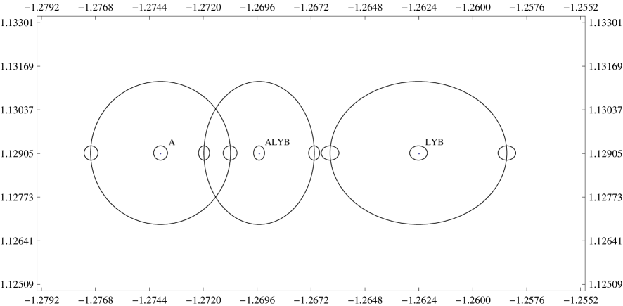
Figure 7: Current $90\%$ CL regions around $\lambda_{\rm LYB}$, $\lambda_{\rm A}$, and $\lambda_{\rm ALYB}$ and $90\%$ CL regions around the central and horizontal border points when $\sigma_{R}$ and $\sigma_{\lambda}$ are cut to $1/10$ of their present values.

Table 14: Values of $V_{\rm ud}$ and $V_{\rm us}$ assuming the central values of $R$ and $\lambda$ are within the small regions displayed in Fig. 7. The $-$ and $+$ indices correspond to the left- and right-hand horizontal border points of each of the larger $90\%$ CL regions in this figure.

$\lambda$	$V_{\rm ud}$	$V_{\rm us}$
$\lambda^{-}_{\rm A}=-1.2770$	$0.96984\pm 0.00020$	$0.24372\pm 0.00078$
$\lambda_{\rm A}=-1.2739$	$0.97180\pm 0.00020$	$0.23575\pm 0.00081$
$\lambda^{+}_{\rm A}=-1.2708$	$0.97378\pm 0.00020$	$0.22745\pm 0.00085$
$\lambda^{-}_{\rm ALYB}=-1.2720$	$0.97303\pm 0.00016$	$0.23062\pm 0.00066$
$\lambda_{\rm ALYB}=-1.2695$	$0.97460\pm 0.00016$	$0.22393\pm 0.00068$
$\lambda^{+}_{\rm ALYB}=-1.2670$	$0.97616\pm 0.00016$	$0.21699\pm 0.00070$
$\lambda^{-}_{\rm LYB}=-1.2663$	$0.97661\pm 0.00025$	$0.2150\pm 0.0011$
$\lambda_{\rm LYB}=-1.2624$	$0.97913\pm 0.00025$	$0.2032\pm 0.0012$
$\lambda^{+}_{\rm LYB}=-1.2585$	$0.98166\pm 0.00025$	$0.1906\pm 0.0013$