Evidence against manifest right-handed currents in neutron beta decay

Abstract

Bounds and presence of manifest right handed currents in neutron beta decay are reviewed. Assuming the unitarity of the Cabibbo-Kobayashi-Maskawa matrix, current experimental situation imposes very stringent limits on the mixing angle, $-0.00077<\zeta<0.00089$, and on the mass eigenstate, $M_{2}({\rm GeV})\in(291.4,439.9)$, in contradiction with the established lower bound on $M_{2}$.

I Introduction

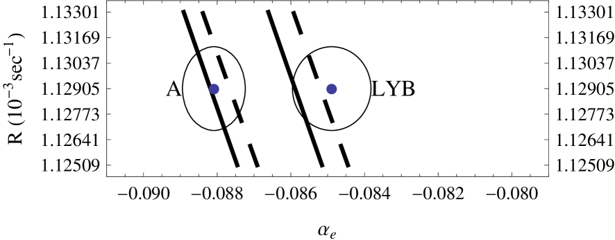
Figure 2: $90\%$ CL SMR (solid lines) and RHCR (dashed lines) with the $V^{\rm NP}_{\rm ud}$ constraint included. The $90\%$ CL region around the current central values of $\alpha^{\rm exp}_{e}$ and $R_{\rm exp}$ are also displayed.

The Standard Model (SM) has its predictive power in neutron beta decay (n$\beta$d) afflicted by the fact that it has two free parameters, namely, $V_{\rm ud}$ and $\lambda=g_{1}/f_{1}$ (the ratio of the two leading form factors at zero momentum transfer). In order to make precise predictions, both parameters should be determined experimentally with great precision. The observables measured with the best precision in free n$\beta$d are the transition rate $R$ and the electron-neutron spin asymmetry $\alpha_{e}$. In superallowed n$\beta$d $V_{\rm ud}$ can be determined very precisely. At present, the problem is that measurements of $\alpha_{e}$ give two incompatible values. Despite this difficulty it is still possible to obtain precise predictions for the region of validity of the SM using the expressions of the SM for $R$ and $\alpha_{e}$ (instead of their experimental values) and the unitarity of the Cabibbo-Kobayashi-Maskawa (CKM) matrix along with the experimental values of $V_{\rm us}$ and $V_{\rm ud}$. This analysis was carried out in Ref. garcia08 and the best prediction of the SM for free n$\beta$d is given in Table II and depictured in Fig. 2(a) of this reference.

In this paper we want to extend this approach to study the bounds and the presence of right handed currents beg77 (RHC) in n$\beta$d. Two new free parameters are introduced, the mixing angle $\zeta$ of $W_{L}$ and $W_{R}$ and the ratio of squares of the masses of the corresponding mass eigenstates $\delta=(M_{1}/M_{2})^{2}$. In addition, we shall use the very precise current measurement of $V_{\rm ud}$ in nuclear physics, which as we shall see plays a very important role.

We have assumed that the CKM matrix is common to $W_{L}$ and $W_{R}$. This is referred to as manifest RHC beg77 .

II Expressions and experimental situation

The SM predicts for the decay rate of n$\beta$d the expression

$$R(10^{-3}\,{\rm s}^{-1})=|V_{\rm ud}|^{2}(0.1897)(1+3\lambda^{2})(1+0.0739\pm 0.0008)$$ (1)

at the level of a precision of $10^{-4}$. The detailed derivation of Eq. (1) is found in Ref. garcia01 . The current experimental value of the neutron mean life pdg08 produces $R_{\rm exp}(10^{-3}\,{\rm s}^{-1})=1.12905(132)$. The theoretical error in $R$ of 0.0008 is included (recently this theoretical bias has been reduced czarnecki04 ; marciano06 ). In our analysis this theoretical error in $R$ is folded into its experimental error bar, $\sigma_{R}=0.00102$ becomes $\sigma^{\prime}_{R}=0.00132$ (in units of $10^{-3}\,{\rm s}^{-1}$). However, it must be stressed that our analysis is independent of $R_{\rm exp}$ and its error bar $\sigma^{\prime}_{R}$ and $\alpha_{e}$. This is true even though the neutron mean life is not yet fully converged serebrov05 and the reason for this is that the analysis of Sec. III to obtain the regions of validity of the SM and the SM with RHC is based on the expressions of $R$ and $\alpha_{e}$ instead of their experimental values.

The advantage of the integrated observables $\alpha_{e}$, $\alpha_{e\nu}$, and $\alpha_{\nu}$, is that their definition entail only kinematics and do not assume any particular theoretical approach. The electron neutrino angular correlation coefficient is defined as $\alpha_{e\nu}=2[N(\theta_{e\nu}<\pi/2)-N(\theta_{e\nu}>\pi/2)]/[N(\theta_{e\nu}<\pi/2)+N(\theta_{e\nu}>\pi/2)]$, where $N(\theta_{e\nu}<\pi/2)$ ($N(\theta_{e\nu}>\pi/2)$) is the number of all events with electron-neutrino pairs emitted in directions that make an angle between them smaller (greater) than $\pi/2$. Similarly the electron-neutron spin asymmetry coefficient is defined as $\alpha_{e}=2[N(\theta_{e}<\pi/2)-N(\theta_{e}>\pi/2)]/[N(\theta_{e}<\pi/2)+N(\theta_{e}>\pi/2)]$, where $\theta_{e}$ is the angle between the electron direction and the polarization direction of the neutron. Analogous definition is used for the neutrino-neutron spin asymmetry $\alpha_{\nu}$. Reference garcia85 provides the complete numerically integrated formulas for the decay rate and angular coefficients.

At the $10^{-4}$ level the SM predicts for the electron-asymmetry the expression garcia06

$$\alpha_{e}=\frac{-0.00021+0.2763\lambda-0.2772\lambda^{2}}{0.1897+0.5692\lambda^{2}}.$$ (2)

We have chosen a negative sign for $\lambda$ to conform with the convention of pdg08 . The important remark here is that there is no theoretical uncertainty in $\alpha_{e}$ at this level of precision. The reason for this is that the uncertainty introduced by the model dependence of the contributions of $Z^{0}$ to the radiative corrections is common to the numerator and denominator of $\alpha_{e}$ and cancels away at the $10^{-4}$ level.

The analysis that leads to Eq. (2) can be extended to the neutrino and electron-neutrino asymmetry coefficients,

$$\alpha_{\nu}=\frac{0.0003-0.3794\lambda-0.2772\lambda^{2}}{0.1897+0.5692\lambda^{2}},$$ (3)

$$\alpha_{e\nu}=\frac{0.1382+0.00054\lambda-0.1393\lambda^{2}}{0.1897+0.5692\lambda^{2}}.$$ (4)

It must be stressed that the angular coefficients are free of a theoretical error at a level of precision of $10^{-4}$. This accuracy is better than the current experimental precision that modern experiments allow. The effects of strong interactions, radiative corrections, and the recoil of the proton have been included garcia06 .

It has remained customary to present experimental results for the old order zero angular coefficients after all the corrections contained in $\alpha_{e}$, $\alpha_{\nu}$, and $\alpha_{e\nu}$, have been applied to the experimental analysis pdg08 ,

$$A_{0}=-\frac{2\lambda(\lambda+1)}{1+3\lambda^{2}},$$ (5)

$$B_{0}=\frac{2\lambda(\lambda-1)}{1+3\lambda^{2}},$$ (6)

$$a_{0}=\frac{1-\lambda^{2}}{1+3\lambda^{2}}.$$ (7)

Also, besides of presenting results for $A_{0}$ it is customary to report directly the value for $\lambda$ obtained from expression (5). Thus, the experimental value of $\lambda$ is free of theoretical uncertainties at the $10^{-4}$ level. We use this value of $\lambda$ in Eq. (2) to estimate the corresponding value of $\alpha_{e}$ and its error bar. By following a similar procedure with eqs. (6) and (3), and (7) and (4), we obtain the numerical values of $\alpha_{\nu}$ and $\alpha_{e\nu}$.

From present experimental results pdg08 for the n$\beta$d order zero angular coefficients, $B_{0}$, $a_{0}$, and $A_{0}$, the corresponding experimental values of the integrated angular coefficients are $\alpha^{\rm exp}_{\nu}=0.9810(30)$, $\alpha^{\rm exp}_{e\nu}=-0.0772(29)$, and the two conflicting values for $\alpha_{e}$, $\alpha^{\rm exp}_{e}({\rm A})=-0.08809(52)$ abele02 ; abele08 and $\alpha^{\rm exp}_{e}({\rm LYB})=-0.08489(65)$ liaud97 ; yerozolimsky97 ; bopp86 .

The expressions of the observables in free n$\beta$d of the SM including the contributions of RHC with a precision of $10^{-4}$ can be expressed as

$$R=(1.0739)A_{\alpha}V_{\text{ud}}^{2}\left(0.1897+(0.5692)B_{\alpha}\lambda^{2}\right),$$ (8)

$$\alpha_{e}=\frac{D_{\alpha}\left(-0.00021-(0.2763)F_{\alpha}\lambda-(0.2772)E_{\alpha}\lambda^{2}\right)}{A_{\alpha}\left(0.1897+(0.5692)B_{\alpha}\lambda^{2}\right)}$$ (9)

$$\alpha_{\nu}=\frac{D_{\alpha}\left(0.0003-(0.3794)F_{\alpha}\lambda+(0.3795)E_{\alpha}\lambda^{2}\right)}{A_{\alpha}\left(0.1897+(0.5692)B_{\alpha}\lambda^{2}\right)}$$ (10)

$$\alpha_{e\nu}=\frac{0.1382+(0.00054)C_{\alpha}\lambda-(0.1393)B_{\alpha}\lambda^{2}}{0.1897+(0.5692)B_{\alpha}\lambda^{2}}.$$ (11)

Here beg77 , $A_{\alpha}\ldots F_{\alpha}$ contain the corrections due to RHC. $A_{\alpha}=2(\eta_{\text{AV}}^{2}+1)/(\eta_{\text{AA}}^{2}+2\eta_{\text{AV}}^{2}+1)$, $B_{\alpha}=(\eta_{\text{AA}}^{2}+\eta_{\text{AV}}^{2})/(\eta_{\text{AV}}^{2}+1)$, $C_{\alpha}=(\eta_{\text{AA}}+\eta_{\text{AV}}^{2})/(\eta_{\text{AV}}^{2}+1)$, $D_{\alpha}=-4\eta_{\text{AV}}/(\eta_{\text{AA}}^{2}+2\eta_{\text{AV}}^{2}+1)$, $E_{\alpha}=\eta_{\text{AA}}$, $F_{\alpha}=(\eta_{\text{AA}}+1)/2$, where $\eta_{\text{AA}}=(\delta+\epsilon^{2})/(\delta\,\epsilon^{2}+1)$, $\eta_{\text{AV}}=-(1-\delta)\epsilon/(\delta\,\epsilon^{2}+1)$, with $\epsilon=(1+\tan{\zeta})/(1-\tan{\zeta})$. The numerical coefficients reamin the same as in eqs. (1)–(4).

III Determination of the regions of validity

The region where the SM and the SM with RHC (SMR and RHCR, respectively) remain valid at a $90\%$ CL are determined by forming a ${\chi}^{2}$ function with the sum of six terms, $((R_{\rm exp}-R)/\sigma^{\prime}_{R})^{2}$, $((\alpha^{\rm exp}_{e}-\alpha_{e})/\sigma_{\alpha_{e({\rm LYB})}})^{2}$, $((\alpha^{\rm exp}_{\nu}-\alpha_{\nu})/\sigma_{\alpha_{\nu}})^{2}$, $((\alpha^{\rm exp}_{e\nu}-\alpha_{e\nu})/\sigma_{\alpha_{e\nu}})^{2}$, $((V^{\rm exp}_{\rm us}-V_{\rm us}\,A^{1/2}_{\alpha})/\sigma_{V_{\rm us}})^{2}$, and $((V^{\rm exp}_{\rm ub}-V_{\rm ub}\,A^{1/2}_{\alpha})/\sigma_{V_{\rm ub}})^{2}$, where $V_{\rm ub}=\sqrt{1-V^{2}_{\rm ud}-V^{2}_{\rm us}}$, and then minimizing the ${\chi}^{2}$ at a lattice of points $(\alpha^{\rm exp}_{e},R_{\rm exp})$ within a rectangle that covers $\pm 3\sigma^{\prime}_{R}$ around $R_{\rm exp}$ and a range for $\alpha^{\rm exp}_{e}$ covering $\alpha^{\rm exp}_{e}({\rm A})$ and $\alpha^{\rm exp}_{e}({\rm LYB})$. The values of $\sigma^{\prime}_{R}$ and $\sigma_{\alpha_{e({\rm LYB})}}$ can also be reduced from their currents values of $0.00132\times 10^{-3}\,{\rm s}^{-1}$ and 0.00065 to one-tenth of these values which run into the theoretical error bars of $10^{-4}$. The free parameters varied at each $(\alpha^{\rm exp}_{e},R_{\rm exp})$ point are $\lambda$, $V_{\rm ud}$, and $V_{\rm us}$ for the SMR and $\lambda$, $V_{\rm ud}$, $V_{\rm us}$, $\zeta$, and $\delta$ for the RHCR. In addition, we shall add a seventh constraint $((V^{\rm exp}_{\rm ud}({\rm NP})-V_{\rm ud}\,A^{1/2}_{\alpha})/\sigma_{V_{\rm ud}})^{2}$ to ${\chi}^{2}$ which incorporates the experimental nuclear physics (NP) value of $V^{\rm exp}_{\rm ud}({\rm NP})=0.97418(27)$.

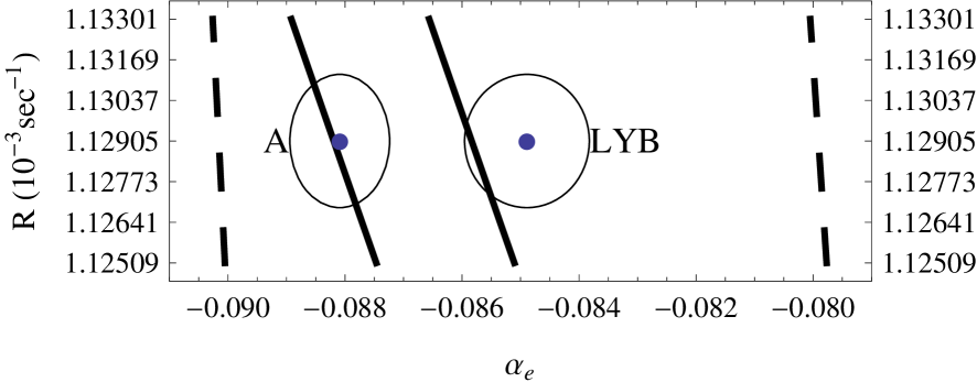
Figure 1: $90\%$ CL SMR (solid lines) and RHCR (dashed lines) without the $V^{\rm NP}_{\rm ud}$ constraint included. The $90\%$ CL region around the current central values of $\alpha^{\rm exp}_{e}$ and $R_{\rm exp}$ are also displayed.

The numerical results are displayed in Table 1 without the $V^{\rm NP}_{\rm ud}$ constraint and in Table 2 with the $V^{\rm NP}_{\rm ud}$ constraint included. The corresponding $90\%$ CL SMR and RHCR are depicted in Figs. 1 and 2.

IV Discussion

In Table 1 the constraint of $V^{\rm NP}_{\rm ud}$ is not enforced, while in Table 2 this constraint is operative. In both tables in each entry the upper numbers obey the constraint of $\alpha^{\rm exp}_{\nu}$ and the lower ones do not obey it. The last two columns give the $90\%$ CL bounds on the two free parameters of manifest RHC.

The $\chi^{2}$ of the SM predictions in both tables show a discrepancy of 2.2 standard deviation. One can see that such a discrepancy is saturated by $\chi^{2}(\alpha_{\nu})$. The presence or absence of the $V^{\rm NP}_{\rm ud}$ constraint plays no role in this discrepancy. When RHC are allowed in, one can appreciate the relevance of $V^{\rm NP}_{\rm ud}$. The bounds on $\zeta$ are reduced and made very uniform when $V^{\rm NP}_{\rm ud}$ constrains $\chi^{2}$. The ranges for $\zeta$ in Table 1 are negative at the top five entries and only in the last two at the bottom $\zeta=0$ is allowed. The length $\Delta\zeta$ of these ranges is around 0.00660. In contrast, in Table 2 the ranges for $\zeta$ are quite symmetric around $\zeta=0$ and have $\Delta\zeta$ of 0.00166, approximately one-fourth of the length when $V^{\rm NP}_{\rm ud}$ is not operative. One can also see in the lower numbers that whether $\alpha^{\rm exp}_{\nu}$ is enforced or not makes no difference. One can, then, conclude that the bounds of $\zeta$, typically of

$$\zeta\in(-0.00077,0.00089)$$ (12)

are imposed solely by $V^{\rm NP}_{\rm ud}$, $V_{\rm us}$, and the unitarity of the CKM matrix. These bounds may be compared with previous ones. In Ref. aquino91 one had $\zeta\in(-0.00060,0.00280)$ with a $\Delta\zeta=0.0340$. The range (12) is more symmetric and has half the length.

The bounds on $\delta$ are practically independent of $V^{\rm NP}_{\rm ud}$, but they are very dependent on $\alpha^{\rm exp}_{\nu}$ as can be seen by comparing the upper and the lower numbers. Actually, the upper bound on $\delta$, at around 0.076 is also almost independent of $\alpha^{\rm exp}_{\nu}$. It is the lower bound on $\delta$ that is very sensitive on $\alpha^{\rm exp}_{\nu}$. In Table 2 it varies from about $\delta\approx 0.033>0$ to about $\delta\approx-0.1020<0$, according to whether $\alpha^{\rm exp}_{\nu}$ is operative or not. Of course, a negative $\delta$ is meaningless and the actual lower bound should be $\delta=0$, which makes the range for $\delta$ an upper bound only. One can conclude that $\alpha^{\rm exp}_{\nu}$ imposes the $90\%$ CL range of

$$\delta\in(0.0334,0.0761)$$ (13)

upon $\delta$.

At this point one should translate (13) into a range for $M_{2}$. One has

$$M_{2}({\rm GeV})\in(291.4,439.9).$$ (14)

Range (14) shows vividly how effective is $\alpha_{\nu}$ for setting an upper bound on $M_{2}$. It also means that manifest RHC are detected in n$\beta$d. However, one already knows that lower bounds on $M_{2}$ have been established. At present one may accept as a conservative lower bound $M_{2}>715$ GeV pdg08 . This is in clear contradiction with range (14).

In order to better understand this situation we have prepared another table, Table 3. We are interested in appreciating what refined measurements of $\alpha^{\rm exp}_{\nu}$ may produce in, hopefully, the near future. We assume that the error bar $\sigma_{\alpha_{\nu}}$ is reduced to one-tenth of its current value. That is, we assume $\sigma_{\alpha_{\nu}}=0.00030$ and we vary the central value $\alpha^{\rm exp}_{\nu}$ from 0.98100 to 0.98760. We keep $R_{\rm exp}$, $V^{\rm exp}_{\rm ud}({\rm NP})$, and $V^{\rm exp}_{\rm us}$ at their current central values and error bars. The results are displayed in Table 3, in steps of 0.00060.

As can be seen in the last column of Table 3, at the $90\%$ CL only when the experimental value of $\alpha_{\nu}$ is greater than 0.9870 the upper bound obtained for $M_{2}$ is not ruled out by its present established lower bound. For $\alpha^{\rm exp}_{\nu}\geq 0.9876$ the central value for $\delta$ is compatible with zero. One can conclude that a clean signal of manifest RHC can be obtained only if future measurements of $\alpha^{\rm exp}_{\nu}$ find it in the range

$$\alpha^{\rm exp}_{\nu}\in(0.9870,0.9876).$$ (15)

V Conclusions

The current experimental situation in n$\beta$d and in the lower bounds on $M_{2}$ lead one to conclude that manifest RHC run into a contradiction, that leads one to conclude that manifest RHC are strongly eliminated as a possibility of physics beyond the SM. The experimental quantity which leads to this conclusion is the current value of $\alpha_{\nu}$.

However, future refined experiments may correct the current situation provided two conditions are met: (1) $\alpha_{\nu}$ is found within range (15) and (2) $\alpha_{e}$ is found in the future in the range $\alpha^{\rm exp}_{e}\in(-0.08570,-0.08717)$ of Table 2. If either of these conditions fail, then manifest RHC will be strongly eliminated. Of course, other forms of new physics could be detected by $\alpha_{\nu}$, as can be appreciated by the values of $\chi^{2}$ in the SM case in Table 3.

As a final remark, it is not idle to emphasize the importance of refined very precise measurements of the observables in n$\beta$d.

Table 1: The minimum of $\chi^{2}$, its corresponding value of $\alpha_{e}$, the prediction for $\alpha_{\nu}$, and the partial contribution from $\alpha_{\nu}$ to $\chi^{2}$ for seven values of $R_{\rm exp}$ (in units of $10^{-3}{\rm sec}^{-1}$) without the $V^{\rm NP}_{\rm ud}$ constraint. The upper numbers obey the constraint of $\alpha^{\rm exp}_{\nu}$ and the lower ones do not obey it. The last two columns give the $90\%$ CL bounds on the two free parameters of manifest RHC, $\zeta$ and $\delta$, respectively.

	SM				RHC
	value		prediction		value		prediction
$R$	$\alpha_{e}$	$\chi^{2}$	$\alpha_{\nu}$	$\chi^{2}(\alpha_{\nu})$	$\alpha_{e}$	$\chi^{2}$	$\alpha_{\nu}$	$\chi^{2}(\alpha_{\nu})$	$\zeta$	$\delta=(M_{1}/M_{2})^{2}$
1.13301	$-$0.08772	5.32	0.98759	4.82	$-$0.08497	$10^{-5}$	0.98100	$10^{-7}$	$(-0.00924,-0.00263)$	$(0.0384,0.0812)$
	$-$0.08772	0.50			$-$0.08497	$10^{-6}$			$(-0.00953,0.00884)$	$(-0.2560,0.1662)$
1.13169	$-$0.08752	5.33	0.98765	4.92	$-$0.08497	$10^{-4}$	0.98100	$10^{-7}$	$(-0.00856,-0.00195)$	$(0.0380,0.0808)$
	$-$0.08749	0.41			$-$0.08497	$10^{-5}$			$(-0.00890,0.00953)$	$(-0.2624,0.1645)$
1.13037	$-$0.08726	5.35	0.98772	5.02	$-$0.08492	$10^{-5}$	0.98100	$10^{-7}$	$(-0.00801,-0.00140)$	$(0.0378,0.0804)$
	$-$0.08723	0.33			$-$0.08492	$10^{-7}$			$(-0.00839,0.01022)$	$(-0.2701,0.1636)$
1.12905	$-$0.08700	5.38	0.98779	5.12	$-$0.08487	$10^{-5}$	0.98100	$10^{-7}$	$(-0.00746,-0.00084)$	$(0.0377,0.0802)$
	$-$0.08700	0.25			$-$0.08487	$10^{-6}$			$(-0.00788,0.01095)$	$(-0.2782,0.1626)$
1.12773	$-$0.08679	5.42	0.98786	5.23	$-$0.08483	$10^{-5}$	0.98100	$10^{-8}$	$(-0.00691,-0.00029)$	$(0.0375,0.0799)$
	$-$0.08676	0.19			$-$0.08483	$10^{-6}$			$(-0.00738,0.01168)$	$(-0.2867,0.1617)$
1.12641	$-$0.08653	5.47	0.98793	5.33	$-$0.08479	$10^{-5}$	0.98100	$10^{-7}$	$(-0.00633,0.00029)$	$(0.0372,0.0796)$
	$-$0.08650	0.14			$-$0.08479	$10^{-5}$			$(-0.00686,0.01251)$	$(-0.2956,0.1607)$
1.12509	$-$0.08627	5.53	0.98799	5.44	$-$0.08473	$10^{-6}$	0.98100	$10^{-9}$	$(-0.00581,0.00082)$	$(0.0371,0.0794)$
	$-$0.08627	0.09			$-$0.08473	$10^{-6}$			$(-0.00638,0.01329)$	$(-0.3055,0.1599)$

Table 2: The minimum of $\chi^{2}$, its corresponding value of $\alpha_{e}$, the prediction for $\alpha_{\nu}$, and the partial contribution from $\alpha_{\nu}$ to $\chi^{2}$ for seven values of $R_{\rm exp}$ (in units of $10^{-3}{\rm sec}^{-1}$) with the $V^{\rm NP}_{\rm ud}$ constraint. The upper numbers obey the constraint of $\alpha^{\rm exp}_{\nu}$ and the lower ones do not obey it. The last two columns give the $90\%$ CL bounds on the two free parameters of manifest RHC, $\zeta$ and $\delta$, respectively.

	SM				RHC
	value		prediction		value		prediction
$R$	$\alpha_{e}$	$\chi^{2}$	$\alpha_{\nu}$	$\chi^{2}(\alpha_{\nu})$	$\alpha_{e}$	$\chi^{2}$	$\alpha_{\nu}$	$\chi^{2}(\alpha_{\nu})$	$\zeta$	$\delta=(M_{1}/M_{2})^{2}$
1.13301	$-$0.08778	5.34	0.98758	4.81	$-$0.08717	0.51	0.98100	$10^{-8}$	$(-0.000785,0.000890)$	$(0.0318,0.0754)$
	$-$0.08775	0.52			$-$0.08717	0.51			$(-0.000769,0.000892)$	$(-0.1011,0.0997)$
1.13169	$-$0.08752	5.35	0.98765	4.91	$-$0.08694	0.42	0.98104	$10^{-4}$	$(-0.000784,0.000891)$	$(0.0320,0.0755)$
	$-$0.08752	0.43			$-$0.08694	0.42			$(-0.000768,0.000892)$	$(-0.1007,0.0992)$
1.13037	$-$0.08726	5.36	0.98772	5.01	$-$0.08668	0.34	0.98102	$10^{-5}$	$(-0.000784,0.000891)$	$(0.0327,0.0758)$
	$-$0.08726	0.35			$-$0.08668	0.34			$(-0.000784,0.000893)$	$(-0.1014,0.1000)$
1.12905	$-$0.08705	5.40	0.98778	5.11	$-$0.08642	0.26	0.98100	$10^{-7}$	$(-0.000768,0.000891)$	$(0.0334,0.0761)$
	$-$0.08702	0.27			$-$0.08642	0.26			$(-0.000768,0.000894)$	$(-0.1020,0.1005)$
1.12773	$-$0.08679	5.44	0.98785	5.22	$-$0.08619	0.20	0.98102	$10^{-5}$	$(-0.000767,0.000892)$	$(0.0337,0.0762)$
	$-$0.08679	0.21			$-$0.08619	0.20			$(-0.000767,0.000894)$	$(-0.1019,0.1004)$
1.12641	$-$0.08653	5.49	0.98792	5.32	$-$0.08596	0.15	0.98104	$10^{-4}$	$(-0.000766,0.000893)$	$(0.0341,0.0764)$
	$-$0.08653	0.15			$-$0.08596	0.14			$(-0.000766,0.000895)$	$(-0.1018,0.1003)$
1.12509	$-$0.08632	5.55	0.98799	5.43	$-$0.08570	0.10	0.98102	$10^{-5}$	$(-0.000766,0.000894)$	$(0.0347,0.0767)$
	$-$0.08629	0.11			$-$0.08570	0.10			$(-0.000766,0.000895)$	$(-0.1024,0.1009)$

Table 3: The minimum of $\chi^{2}$, its corresponding value of $\alpha_{e}$, the prediction for $\alpha_{\nu}$, and the partial contribution from $\alpha_{\nu}$ to $\chi^{2}$ for several values of $\alpha^{\rm exp}_{\nu}$ with the error bar $\sigma_{\alpha_{\nu}}$ reduced to one-tenth of its current value. $R_{\rm exp}$, $V^{\rm exp}_{\rm ud}({\rm NP})$, and $V^{\rm exp}_{\rm us}$ are kept at their current central values and error bars. The last three columns give the $90\%$ CL bounds on the two free parameters of manifest RHC, $\zeta$ and $\delta$, and the corresponding bounds on $M_{2}$, respectively.

	SM				RHC
	value		prediction		value		prediction
$\alpha_{\nu}$	$\alpha_{e}$	$\chi^{2}$	$\alpha_{\nu}$	$\chi^{2}(\alpha_{\nu})$	$\alpha_{e}$	$\chi^{2}$	$\alpha_{\nu}$	$\chi^{2}(\alpha_{\nu})$	$\zeta$	$\delta=(M_{1}/M_{2})^{2}$	$M_{2}\,({\rm GeV})$
0.9810	$-$0.08840	482.99	0.98740	454.85	$-$0.08642	0.26	0.9810	$10^{-9}$	$(-0.000768,0.000891)$	$(0.0564,0.0609)$	$(325.8,338.5)$
0.9816	$-$0.08827	401.45	0.98743	378.08	$-$0.08648	0.26	0.9816	$10^{-8}$	$(-0.000767,0.000891)$	$(0.0536,0.0583)$	$(332.9,347.2)$
0.9822	$-$0.08817	327.38	0.98747	308.23	$-$0.08653	0.26	0.9822	$10^{-8}$	$(-0.000767,0.000890)$	$(0.0507,0.0556)$	$(340.9,357.0)$
0.9828	$-$0.08804	260.98	0.98750	245.69	$-$0.08658	0.26	0.9828	$10^{-7}$	$(-0.000766,0.000889)$	$(0.0476,0.0528)$	$(349.8,368.5)$
0.9834	$-$0.08791	202.05	0.98754	190.19	$-$0.08663	0.26	0.9834	$10^{-7}$	$(-0.000766,0.000889)$	$(0.0443,0.0498)$	$(360.2,381.9)$
0.9840	$-$0.08780	150.65	0.98757	141.71	$-$0.08668	0.26	0.9840	$10^{-7}$	$(-0.000765,0.000888)$	$(0.0407,0.0467)$	$(372.0,398.5)$
0.9846	$-$0.08767	106.80	0.98761	100.40	$-$0.08674	0.26	0.9846	$10^{-7}$	$(-0.000765,0.000887)$	$(0.0368,0.0433)$	$(386.3,419.1)$
0.9852	$-$0.08754	70.49	0.98764	66.20	$-$0.08679	0.26	0.9852	$10^{-7}$	$(-0.000764,0.000887)$	$(0.0324,0.0396)$	$(404.0,446.6)$
0.9858	$-$0.08741	41.72	0.98768	39.09	$-$0.08684	0.26	0.9858	$10^{-7}$	$(-0.000764,0.000886)$	$(0.0273,0.0355)$	$(426.7,486.5)$
0.9864	$-$0.08731	20.49	0.98771	19.05	$-$0.08689	0.26	0.9864	$10^{-7}$	$(-0.000763,0.000885)$	$(0.0211,0.0310)$	$(456.6,553.4)$
0.9870	$-$0.08718	6.80	0.98774	6.15	$-$0.08694	0.26	0.9870	$10^{-7}$	$(-0.000762,0.000868)$	$(0.0119,0.0256)$	$(502.4,736.9)$
0.9876	$-$0.08705	0.65	0.98778	0.35	$-$0.08702	0.26	0.9876	$10^{-7}$	$(-0.000758,0.000884)$	$(-0.0187,0.0187)$	$>587.9$