Isospectral surfaces with distinct covering spectra via Cayley Graphs

Abstract.

The covering spectrum is a geometric invariant of a Riemannian manifold, more generally of a metric space, that measures the size of its one-dimensional holes by isolating a portion of the length spectrum. In a previous paper we demonstrated that the covering spectrum is not a spectral invariant of a manifold in dimensions three and higher. In this article we give an example of two isospectral Cayley graphs that admit length space structures with distinct covering spectra. From this we deduce the existence of infinitely many pairs of Sunada-isospectral surfaces with unequal covering spectra.

1. Introduction

The covering spectrum of a complete length space $X$ is a geometric invariant introduced by Sormani and Wei [SW] that measures the size of one dimensional holes in $X$ by isolating the lengths of certain closed geodesics that are minimal in their free homotopy class. More specifically, the covering spectrum can be computed by considering a certain family $\{\widetilde{X}^{\delta}\}_{\delta>0}$ of regular coverings of $X$, where $\widetilde{X}^{\delta}$ covers $\widetilde{X}^{\delta^{\prime}}$ for $\delta^{\prime}>\delta$. The covering spectrum of $X$ then consists of those values of $\delta$ where the isomorphism type of the cover changes. That is, the covering spectrum is the collection of $\delta$’s where there is a “jump” in the step function $\delta\mapsto\widetilde{X}^{\delta}$. One can see that a “jump” at time $\delta$ corresponds to the appearance of a “hole” of circumference $2\delta$ or, in the case of manifolds, a non-trivial free homotopy class whose shortest geodesic is of length $2\delta$ (cf. Proposition 2.4).

As an example, we follow [SW, Example 2.5] and consider the flat $2\times 3$ torus $X=S^{1}(2)\times S^{1}(3)$, where $S^{1}(c)$ denotes the circle of circumference $c$. One can see through the covering spectrum algorithm (see 2.7) that the $\delta$-covers of $X$ are given by $\widetilde{X}^{\delta}=\mathbb{R}^{2}$ (for $0<\delta\leq 1$), $\widetilde{X}^{\delta}=S^{1}(2)\times\mathbb{R}$ (for $1<\delta\leq\frac{3}{2}$ ) and $\widetilde{X}^{\delta}=X$ (for $\delta>\frac{3}{2}$). Hence, the covering spectrum of $X$ is given by $\{1,\frac{3}{2}\}$. Each of these numbers is the circumference of a “hole” in this torus and also half the length of the minimal closed geodesics in the free homotopy classes associated to the standard generators $(1,0)$ and $(0,1)$ in $\pi_{1}(X)=\mathbb{Z}\times\mathbb{Z}$.

As there is a long-standing interest in the relationship between the Laplace spectrum of a manifold and its length spectrum (i.e., the collection of lengths of closed geodesics), it is natural to wonder about the mutual influences between the Laplace spectrum and the covering spectrum. Specifically, one would like to know if the covering spectrum is a spectral invariant. In [SW, Ex. 10.5], Sormani and Wei demonstrated that certain isospectral manifolds arising through Sunada’s method [Sun] share the same covering spectrum, suggesting that the covering spectrum might at least be an invariant of this technique. However, through an analysis of the group theory and geometry underlying the covering spectrum we constructed Sunada-isospectral manifolds with distinct covering spectra in dimensions three and higher [DGS, Sec. 8], thus showing that the covering spectrum is not a spectral invariant.

Indeed, we recall that a triple of finite groups $(G,H_{1},H_{2})$, where $H_{1}$ and $H_{2}$ are subgroups of $G$, is said to be a Gassmann-Sunada triple if for any conjugacy class $C\subset G$ the sets $C\cap H_{1}$ and $C\cap H_{2}$ are of the same order. If $(G,H_{1},H_{2})$ is a Gassmann-Sunada triple where $G$ acts freely and isometrically on a Riemannian manifold $M$, then Sunada’s theorem (Theorem 4.1) tells us that the quotient Riemannian manifolds $H_{1}\backslash M$ and $H_{2}\backslash M$ are isospectral, and the isospectral pairs arising in this manner are said to be Sunada-isospectral. Sunada’s theorem provided the first systematic method for constructing isospectral manifolds and—along with its numerous variants—accounts for many of the isospectral pairs in the literature (see [G] for a retrospective on Sunada’s method). In [DGS] we discovered an analogous algebraic condition and theorem concerning the covering spectrum. Specifically, we showed the following.

1.1 Theorem ([DGS] Theorem 2.2).

Let $(G,H_{1},H_{2})$ be a triple of finite groups, where $H_{1}$ and $H_{2}$ are subgroups of $G$, and suppose $G$ acts freely on a closed manifold $M$. If $M$ is simply-connected and of dimension at least $3$, then the following are equivalent:

1. $H_{1}$ and $H_{2}$ are jump equivalent subgroups of $G$; that is, for any subsets $S,T\subset G$ that are stable under conjugation we have

   $$\langle H_{1}\cap S\rangle=\langle H_{1}\cap T\rangle\Longleftrightarrow\langle H_{2}\cap S\rangle=\langle H_{2}\cap T\rangle.$$

   In which case we say that $(G,H_{1},H_{2})$ is a jump triple.

2. For every $G$-invariant Riemannian metric on $M$, the quotient Riemannian manifolds $H_{1}\backslash M$ and $H_{2}\backslash M$ share the same covering spectrum.

We then went on to produce examples of Gassmann-Sunada triples that are not jump triples. As a consequence we were able to construct Sunada-isospectral manifolds with distinct covering spectra in all dimensions greater than or equal to three. However, our method for building such examples appears to fail in dimension two as the arguments underlying Theorem 1.1 depend in part on the fact that all free homotopy classes in dimension three and higher can be represented by simple closed curves.

In this article we take a different approach in order to establish the following theorem showing that the covering spectrum is not a spectral invariant of a surface.

1.2 Theorem.

For each integer $n\geq 1$ there exist pairs of closed connected Sunada-isospectral surfaces of genus $7n+1$ with distinct covering spectra.

To prove the result above we construct certain Cayley graphs associated to a well-known Gassmann-Sunada triple [Bu, Ex. 11.4.7.], and endow them with suitably chosen edge lengths so that the resulting length spaces $X_{1}$ and $X_{2}$ have distinct covering spectra. We then build continuous families of Riemannian manifolds $\{(M_{1},g_{1}^{\epsilon})\}_{\epsilon>0}$ and $\{(M_{2},g_{2}^{\epsilon})\}_{\epsilon>0}$ that are pairwise Sunada-isospectral for each $\epsilon>0$ and such that for each $i=1,2$ the family $(M_{i},g_{i}^{\epsilon})$ converges with respect to the Gromov-Hausdorff metric to $X_{i}$ as $\epsilon$ tends to zero. Then, since the covering spectrum is continuous under Gromov-Hausdorff convergence [SW, Corollary 8.5], it follows that for $\epsilon$ sufficiently small $(M_{1},g_{1}^{\epsilon})$ and $(M_{2},g_{2}^{\epsilon})$ are Sunada-isospectral manifolds with distinct covering spectra.

Currently, it is not clear to us whether any of the aforementioned pairs consist of Riemann surfaces. It would appear to be an interesting problem to determine whether the covering spectrum is a spectral invariant among such spaces.

The outline of this article is as follows. In Section 2 we will formulate the precise definition of the covering spectrum, present a useful algorithm for computing it, and discuss its behavior under Gromov-Hausdorff convergence. In Section 3 we recall the notion of a Cayley graph, we produce the length spaces $X_{1}$ and $X_{2}$ mentioned above, and show their covering spectra are distinct. In Section 4 we review how the Cayley graphs relate to the isospectral problem, and we finish the proof of Theorem 1.2 as outlined.

2. The Covering Spectrum

In this section we will recall the definition of the covering spectrum as given in [SW]. Since the primary focus of this paper will be the covering spectra of compact semi-locally simply-connected length spaces we will only formulate our definition in this setting. However, we note that in [DGS] we extended this definition of the covering spectrum to arbitrary metric spaces.

We will begin by recalling the notion of a filtration of a group.

2.1 Definition.

Let $G$ be a group. A filtration $\operatorname{Fil}^{\bullet}G$ of $G$ is a family $\{\operatorname{Fil}^{i}G\}_{i\in I}$ of subgroups of $G$, where $i$ ranges over an ordered index set $I$, such that $\operatorname{Fil}^{i}G\subset\operatorname{Fil}^{j}G$ whenever $i<j$. The jump set of the filtration is the subset of $I$ given by

$$\operatorname{Jump}(\operatorname{Fil}^{\bullet}G)=\{i\in I:\operatorname{Fil}^{i}G\neq\operatorname{Fil}^{j}G\mbox{ for all }j>i\}.$$

2.2 Example (Filtrations Induced by Class Functions).

Let $G$ be a group and $m:G\to\mathbb{R}_{\geq 0}$ a class function; i.e., $m$ is constant on the conjugacy classes of $G$. Then $m$ induces a filtration $\operatorname{Fil}^{\bullet}_{m}G=\{\operatorname{Fil}^{\delta}_{m}G\}_{\delta>0}$, where

$$\operatorname{Fil}^{\delta}_{m}G:=\langle g\in G:m(g)<\delta\rangle.$$

Such filtrations will prove to be useful in our discussion of the covering spectrum.

We now observe that given a connected and compact semi-locally simply-connected length space $(X,d)$ its metric structure induces a natural filtration (indexed by the positive reals) on its fundamental group $\pi_{1}(X,x_{0})$. Indeed, for each $\delta>0$ let $\mathcal{U}_{\delta}$ be the open cover of $X$ consisting of all the open $\delta$-balls in $(X,d)$. Then let $\operatorname{Fil}^{\delta}\pi_{1}(X,x_{0})$ be the subgroup of $\pi_{1}(X,x_{0})$ generated by classes of the form $[\alpha*\beta*\bar{\alpha}]$, where $\beta:[0,1]\to X$ is a loop that is completely contained in some open $\delta$-ball, $\alpha$ is a path from $x_{0}$ to $\beta(0)$ and $\bar{\alpha}(t)=\alpha(1-t)$ is its reverse. The subgroup $\operatorname{Fil}^{\delta}\pi_{1}(X,x_{0})$ is normal in $\pi_{1}(X,x_{0})$ and the conjugacy classes of the generators $[\alpha*\beta*\bar{\alpha}]$ of $\operatorname{Fil}^{\delta}\pi_{1}(X,x_{0})$ represent the free homotopy classes of loops that have representatives completely contained in a $\delta$-ball. In this fashion we obtain a filtration $\operatorname{Fil}^{\bullet}\pi_{1}(X,x_{0})=\{\operatorname{Fil}^{\delta}\pi_{1}(X,x_{0})\}_{\delta>0}$ of $\pi_{1}(X,x_{0})$.

2.3 Definition.

Let $(X,d)$ be a connected and compact semi-locally simply-connected length space. We then define the covering spectrum of $(X,d)$ to be the set

$$\operatorname{CovSpec}(X,d)=\operatorname{Jump}(\operatorname{Fil}^{\bullet}\pi_{1}(X,x_{0})).$$

Now, since each subgroup $\operatorname{Fil}^{\delta}\pi_{1}(X,x_{0})$ of $\pi_{1}(X,x_{0})$ is normal, the Galois theory of covering spaces [Sp, Theorem 2.5.13] tells us that we may associate to each subgroup a connected regular covering space $\widetilde{X}^{\delta}\to X$ known as the $\delta$-cover of $X$. The $\delta$-cover has the property that if $Y\to X$ is any covering space that evenly covers every $\delta$-ball of $X$, then $\widetilde{X}^{\delta}$ is a covering space of $Y$ (cf. [Sp, Lemma 2.5.11]). Hence, we obtain a tower $\{\widetilde{X}^{\delta}\}_{\delta>0}$ of regular covers of $X$ and the covering spectrum detects when we have a change in the isomorphism type of the cover. That is, $\delta\in\operatorname{CovSpec}(X,d)$ if and only if for all $\epsilon>\delta$, $\widetilde{X}^{\epsilon}$ and $\widetilde{X}^{\delta}$ are non-isomorphic as covering spaces. In the event that we are considering a compact Riemannian manifold $(M,g)$ we see that the covering spectrum also contains information about the length spectrum.

2.4 Proposition ([DGS] Corollary 4.5).

Let $(M,g)$ be a closed Riemannian manifold. Then

1. $2\operatorname{CovSpec}(M,g)$ is a subset of the length spectrum.

2. if $\delta\in\operatorname{CovSpec}(M,g)$, then $2\delta$ is the length of the shortest (smoothly) closed geodesic in $(M,g)$ that has a lift to $\widetilde{M}^{\delta}$ that is not a closed loop.

In order to compute the length spectrum it will be useful to introduce the minimum marked length map.

2.5 Definition.

Let $(X,d)$ be a connected and compact semi-locally simply-connected length space with fundamental group $\pi_{1}(X)$ and simply-connected universal cover $(\widetilde{X},\tilde{d})$. Then the minimum marked length map $m:\pi_{1}(X)\to\mathbb{R}_{\geq 0}$ is given by

$$m([\gamma])\equiv\inf_{\tilde{x}\in\widetilde{X}}\tilde{d}(\tilde{x},\gamma\cdot\tilde{x}),$$

where $\pi_{1}(X)$ acts on $\widetilde{X}$ via deck transformations.

The minimum marked length map $m:\pi_{1}(X)\to\mathbb{R}_{\geq 0}$ assigns to each $[\gamma]\in\pi_{1}(X)$ the length of the shortest closed geodesic in the free homotopy class determined by $[\gamma]$. Since free homotopy classes correspond to conjugacy classes in $\pi_{1}(X)$ we see that $m$ is a class function. Hence, by Example 2.2 $m$ induces the filtration $\operatorname{Fil}^{\bullet}_{m}\pi_{1}(X)$ and we have the following.

2.6 Proposition (cf. [DGS] Proposition 2.5).

Let $(X,d)$ be a connected and compact semi-locally simply-connected length space with minimum marked length map $m:\pi_{1}(X)\to\mathbb{R}_{\geq 0}$. Then

$$\operatorname{CovSpec}(X,d)=\frac{1}{2}\operatorname{Jump}(\operatorname{Fil}^{\bullet}_{m}\pi_{1}(X)).$$

The above leads to the following algorithm for computing the covering spectrum of a compact semi-locally simply-connected length space as found in [SW, p. 54] and [DGS, 4.6].

2.7 Covering Spectrum Algorithm.

Let $(X,d)$ be a compact semi-locally simply-connected length space with minimum marked length map $m:\pi_{1}(X)\to\mathbb{R}_{\geq 0}$. Then let

$$\begin{array}[]{l}\delta_{1}=\inf\{m(\sigma)\colon\sigma\in\pi_{1}(X),\sigma\neq 1\}>0\\ \delta_{2}=\inf\{m(\sigma)\colon\sigma\in\pi_{1}(X),\sigma\not\in\langle\tau\in\pi_{1}(X)\colon\;m(\tau)\leq\delta_{1}\rangle\}>\delta_{1}\\ \delta_{3}=\inf\{m(\sigma)\colon\sigma\in\pi_{1}(X),\sigma\not\in\langle\tau\in\pi_{1}(X)\colon\;m(\tau)\leq\delta_{2}\rangle\}>\delta_{2}\\ \cdots\end{array}$$

where we continue until $\langle\sigma\in\pi_{1}(X)\colon\;m(\sigma)\leq\delta_{r}\rangle=\pi_{1}(X)$. Now since $X$ is a compact length space we know by [SW, Lemma 4.6] that the image of $m$ is closed and discrete. It then follows from the fact that $\pi_{1}(X)$ is finitely generated that the above process stops in finitely many steps at some $\delta_{r}$, and by the previous proposition we see

$$\operatorname{CovSpec}(X,d)=\{\frac{1}{2}\delta_{1},\ldots,\frac{1}{2}\delta_{r}\}.$$

2.8 Remark.

For an application of the covering spectrum algorithm to the case of flat tori the reader is encouraged to see [DGS, Example 4.7]. In particular, this example shows that for a flat $n$-torus, the covering spectrum need not be equal to the successive minima of the corresponding lattice $\mathcal{L}$ in $\mathbb{R}^{n}$.

We conclude this section by recalling that in Proposition 2.4 we observed that for any compact length space $X$ we have $2\operatorname{CovSpec}(X)\subset\operatorname{Spec_{L}}(X)$, where $\operatorname{Spec_{L}}(X)$ denotes the length spectrum of $X$. Now, it is well known that the length spectrum does not behave well under Gromov-Hausdorff convergence: lengths may disappear or suddenly appear in the limit (cf. [SW, Examples 8.1-8.3]). However, in Section 3 we will use the fact that, in contrast, the covering spectrum is continuous under Gromov-Hausdorff convergence.

2.9 Proposition ([SW] Corollary 8.5).

If $X_{i}$ is a sequence of compact length spaces converging to a compact length space $Y$ in the Gromov-Hausdorff sense, then the covering spectra converge in the Hausdorff sense as subsets of $\mathbb{R}$. That is, if $X_{i}\stackrel{{\scriptstyle\rm{GH}}}{{\longrightarrow}}Y$, then

$$\lim_{i\to\infty}d_{H}(\operatorname{CovSpec}(X_{i})\cup\{0\},\operatorname{CovSpec}(Y)\cup\{0\})=0,$$

where $d_{H}$ denotes the Hausdorff distance between subsets of $\mathbb{R}$.

Hence, twice the covering spectrum determines a part of the length spectrum of a compact length space that behaves well under Gromov-Hausdorff convergence.

2.10 Remark.

We refer the reader to Sections 7 and 8 of [SW] for the relevant details on Gromov-Hausdorff convergence and the proof of the proposition above.

3. Cayley Graphs associated to the Fano plane

In this section we will introduce certain Cayley graphs and associated length spaces. In the next section we will use these examples to construct isospectral surfaces with distinct covering spectra.

By a graph we will mean a quadruple $(V,E,o,t)$ where $V$ and $E$ are the sets of vertices and edges (respectively), and $o$ and $t$ are maps from $E$ to $V$ associating to each edge its origin and target. In other words, we consider directed graphs with possible self-edges and multiple edges between the same vertices. A morphism $f$ from a graph $(V,E,o,t)$ to a graph $(V^{\prime},E^{\prime},o^{\prime},t^{\prime})$ is a pair of maps $f_{v}\colon\;V\to V^{\prime}$ and $f_{e}\colon\;E\to E^{\prime}$ for which $o^{\prime}\circ f_{e}=f_{v}\circ o$ and $t^{\prime}\circ f_{e}=f_{v}\circ t$.

If $G$ is a group acting on the right on a set $V$, and $S\subset G$ is a subset, then we can consider the (generalized) Cayley graph $V[S]=(V,E,o,t)$ associated to $V$ and $S$, where $E=V\times S$ with $o(v,s)=v$ and $t(v,s)=vs$. Note that we can label the edges by $S$ according to their second coordinate—this will be referred to as the color or type of the edge—and that for every $s\in S$ every vertex has a single incoming and outgoing edge of type $s$.

If for $V$ we take a finitely generated group $G$ with the $G$-action by right multiplication and we let $S$ be a set of generators of $G$, then we obtain the usual Cayley graph $G[S]$ of the group $G$ (cf. [dH, Chp. 4]). The group $G$ then has a left-action by graph automorphisms on $G[S]$ where $G$ acts on the vertices by left multiplication. The action preserves the labeling of the edges by $S$. For any subgroup $H$ of $G$ the quotient graph $H\backslash(G[S])$ is then naturally isomorphic to the generalized Cayley graph $(H\backslash G)[S]$. The graph $(H\backslash G)[S]$ is also known as the Schreier graph associated to $H\backslash G$ and $S$ (cf. [dH, Chp. 4]).

In our application, the group $G$ will be the group $G=\operatorname{Gl}_{3}(\mathbb{F}_{2})$, which we will consider with its right action on the Fano plane, the projective plane over the field $\mathbb{F}_{2}$ of $2$ elements. The set $V_{1}$ of points of the Fano plane is labeled by non-zero row vectors of length $3$ over $\mathbb{F}_{2}$, which are multiplied on the right by matrices in $G$. A second set $V_{2}$ with right $G$-action that we will consider is the set of lines in the Fano plane. We can label $V_{2}$ by the same set of non-zero vectors in $\mathbb{F}_{2}^{3}$ where the line through two distinct points $v_{1},v_{2}\in V_{1}$ is labeled by the unique nonzero vector $w\in\mathbb{F}_{2}^{3}$ so that $\langle v_{1},w\rangle=\langle v_{2},w\rangle=0$ under the standard inner product $\langle\cdot,\cdot\rangle$ on $\mathbb{F}_{2}^{3}$; see Figure 1. By computing the stabilizer in $G$ of the element represented by $100$ in each of $V_{1}$ and $V_{2}$ we see that we have $G$-set isomorphisms $V_{1}\cong H_{1}\backslash G$, and $V_{2}\cong H_{2}\backslash G$, where

$$H_{1}=\left(\begin{array}[]{ccc}1&0&0\\ &*&*\\ &*&*\end{array}\right)\mbox{ and }H_{2}=\left(\begin{array}[]{ccc}1&*&*\\ 0&*&*\\ 0&*&*\end{array}\right).$$

Let us now consider the subset $S=\{A,B\}\subset G=\operatorname{Gl}_{3}(\mathbb{F}_{2})$ consisting of the two matrices

$$A=\left(\begin{array}[]{rrr}1&1&0\\ 0&0&1\\ 0&1&0\end{array}\right),\qquad B=\left(\begin{array}[]{rrr}0&1&0\\ 0&0&1\\ 1&0&0\end{array}\right).$$

The action of $A$ on the Fano plane is given by dotted arrows in Figure 1, while the action of $B$ is rotation by 120 degrees counterclockwise. By rearranging the vertices we see that the Cayley graph $V_{1}[A,B]$ is the graph in Figure 2 where the dotted arrows indicate edges associated to $A$ and the solid arrows indicate edges associated to $B$. By tracking the action of $A$ and $B$ on the lines of the Fano plane (or on the three points each line contains) we construct the Cayley graph $V_{2}[A,B]$ as in Figure 3. These graphs are also given in [Bu, Ex. 11.4.7] and [Br].

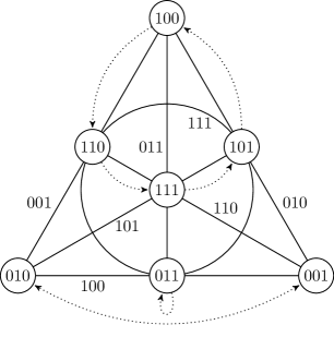
Figure 1. The Fano plane with seven points and seven lines, with the action of the matrix $A$ given by dotted arrows.

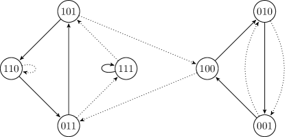
Figure 2. The Cayley graph $V_{1}[A,B]=H_{1}\backslash G[A,B]$ of $A$ and $B$ acting on the points in the Fano plane.

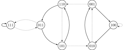
Figure 3. The Cayley graph $V_{2}[A,B]=H_{2}\backslash G[A,B]$ of $A$ and $B$ acting on the lines in the Fano plane.

The geometric realization of a graph $(V,E,o,t)$ is the topological space that one obtains by glueing closed intervals onto the set $V$ as follows: for each $e\in E$ one adds an interval $[0,1]$ identifying $0$ with $o(e)\in V$ and $1$ with $t(e)\in V$. If one designates a positive real number $l_{e}$ as the length of an edge $e$ then one can give the interval assocated to $e$ length $l_{e}$ and in this way one obtains a length space.

For our Cayley graph $G[A,B]$ we will assign a length $l_{A}>0$ to all edges associated with $A$ and $l_{B}>0$ to all edges associated with $B$, and we thus obtain a length space $X(l_{A},l_{B})$. The group $G$ acts by isometries on $X(l_{A},l_{B})$ and it acts freely, i.e., no non-trivial element of $G$ has a fixed point on $X(l_{A},l_{B})$. The quotient length space $H_{1}\backslash X(l_{A},l_{B})$ is the length space $X_{1}$ associated to $V_{1}[A,B]$ and $H_{2}\backslash X(l_{A},l_{B})$ is the length space $X_{2}$ associated to $V_{2}[A,B]$.

3.1 Proposition.

If $0<l_{A}<l_{B}<\frac{3}{2}l_{A}$, then $l_{A}+\frac{1}{2}l_{B}$ lies in the covering spectrum of $X_{1}=H_{1}\backslash X(l_{A},l_{B})$ but not in the covering spectrum of $X_{2}=H_{2}\backslash X(l_{A},l_{B})$.

Proof.

We see from the assumption that

$$l_{A}<l_{B}<2l_{A}<l_{A}+l_{B}<2l_{B}<3l_{A}<2l_{A}+l_{B}$$

represent the lengths of the non-trivial minimal loops of length below $l_{A}+2l_{B}$. These lengths form the first column of the table in Figure 4.

The second and third column in the table lists closed loops in $X_{1}$ and $X_{2}$ of the given lengths. In this table $A_{001}$ denotes the path along the edge associated to $A$ leaving from the vertex with label $001$. One has to inspect the appropriate graph to see what the endpoint of $A_{001}$ is: in $X_{1}$ it is $010$ and in $X_{2}$ it is $110$. Paths are composed according to the following convention: if the endpoint of a path $p$ is the starting point of a path $q$ then $p*q$ runs through $p$ at double speed on the interval $[0,1/2]$ and then through $q$ on $[1/2,1]$.

By inspecting the graphs in Figures 2 and 3 one deduces that every closed loop in $X_{1}$ or $X_{2}$ that is of length below $l_{A}+2l_{B}$, is freely homotopic to either a constant loop, or to a loop in the table, or to the inverse of a loop in the table in Figure 4. Note also that the lengths of the loops in the table are minimal within their free homotopy class.

length	$X_{1}=H_{1}\backslash X(l_{A},l_{B})$	$X_{2}=H_{2}\backslash X(l_{A},l_{B})$
$l_{A}$	$\sigma_{1}=A_{110}$	$\tau_{1}=A_{100}$
$l_{B}$	$\sigma_{2}=B_{111}$	$\tau_{2}=B_{111}$
$2l_{A}$	$\sigma_{1}^{2}$	$\tau_{1}^{2}$
	$\sigma_{3}=A_{010}*A_{001}$	$\tau_{3}=A_{111}*A_{011}$
$l_{A}+l_{B}$	$\sigma_{4}=B_{010}*A_{001}$	$\tau_{4}=A_{010}*B_{010}^{-1}$
	$\sigma_{5}=B_{010}*A_{010}^{-1}$	$\tau_{5}=A_{110}*B_{101}$
$2l_{B}$	$\sigma_{2}^{2}$	$\tau_{2}^{2}$
$3l_{A}$	$\sigma_{1}^{3}$	$\tau_{1}^{3}$
$2l_{A}+l_{B}$	$\sigma_{6}=B_{011}*A_{101}*A_{100}$	$\tau_{2}*\tau_{3}$
	$\sigma_{7}=B_{011}*A_{111}^{-1}*A_{011}^{-1}$	$\tau_{2}*\tau_{3}^{-1}$

Figure 4. The minimal loops in $X_{1}$ and $X_{2}$ of length below $l_{A}+2l_{B}$

Denoting the minimum marked length map for $X_{2}$ by $m$ one sees that $\operatorname{Fil}_{m}^{2l_{A}+l_{B}}(\pi_{1}(X_{2}))$ is the normal subgroup of $\pi_{1}(X_{2})$ generated by all homotopy classes of loops that are freely homotopic to one of $\tau_{1},\ldots,\tau_{5}$, which is also equal to $\operatorname{Fil}_{m}^{2l_{A}+l_{B}+\epsilon}(\pi_{1}(X_{2}))$ for any $0<\epsilon\leq l_{B}-l_{A}$. We deduce that $2l_{A}+l_{B}$ is not a jump of the filtration $\operatorname{Fil}_{m}^{\bullet}\pi_{1}(X_{2})$, so that by Proposition 2.6 the number $l_{A}+\frac{1}{2}l_{B}$ is not in the covering spectrum of $X_{2}$.

To complete the proof we will show that the class $c$ in $\pi_{1}(X_{1},x_{0})$ of any loop in $X_{1}$ based at $x_{0}$, that is freely homotopic to $\sigma_{6}$, does not lie in the normal subgroup $N$ of $\pi_{1}(X_{1},x_{0})$ generated by the classes of all loops based at $x_{0}$ that are freely homotopic to one of $\sigma_{1},\ldots,\sigma_{5}$. To see this, consider the topological quotient space $K$ of $X_{1}$ that one obtains by contracting the loops $\sigma_{1},\ldots,\sigma_{5}$ to a point. Then $N$ lies in the kernel of the induced group homomorphism $\pi_{1}(X_{1})\to\pi_{1}(K)$, but one sees from the graph in Figure 2 that $c$ does not map to the trivial class. Since $\sigma_{6}$ has length $2l_{A}+l_{B}$, and this length is minimal in its free homotopy class, it follows with Proposition 2.6 that $l_{A}+\frac{1}{2}l_{B}$ lies in the covering spectrum of $X_{1}$. ∎

4. From Cayley graphs to isospectral surfaces

Suppose that $G$ is a group and $S$ is a subset of $G$. For any set $V$ with a right action of $G$ we defined the Cayley graph $V[S]$ with vertex set $V$ and edge set $E$ consisting of an edge from $x$ to $xs$ for each $s\in S$ and $x\in V$. We can construct a surface out of this graph as follows (cf. [Bu, Chapter 11]).

Suppose that we have a compact connected surface of genus $g$. If $n=\#S$, then we add $n$ handles to the surface, and on this surface $M$ we choose a Riemannian metric. We now cut open the handles to obtain a compact surface $M^{\prime}$ with $2n$ border components $\{B_{s},\overline{B}_{s}\colon\;s\in S\}$, where for each $s\in B$ a homeomorphism $B_{s}\to\overline{B}_{s}$ is given so that identifying $B_{s}$ with $\overline{B}_{s}$ for all $s\in S$ gives us $M$. In Figure 5 this is illustrated for $g=0$ and $n=2$.

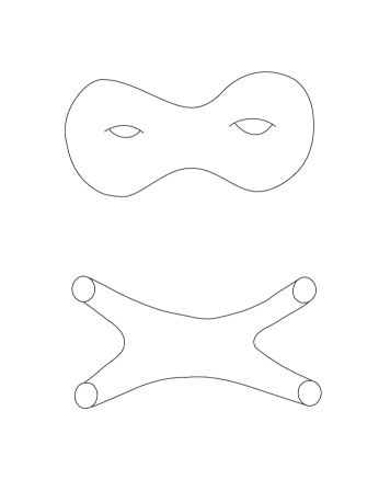
Figure 5. Cutting a surface of genus two along two curves

With this building block we can now make a surface as follows. Take the surface $M^{\prime}\times V$ and for every edge from an element $x\in V$ to $xs\in V$ of color $s\in S$ we identify $B_{s}\times\{x\}$ with $\overline{B}_{s}\times\{xs\}$ using the homeomorphism $B_{s}\to\overline{B}_{s}$. We will denote this quotient by $M[V;S]$. It is a compact surface, and it is not hard to see that if $V[S]$ is connected, then the genus of $M[V;S]$ is $1+(g+n-1)\#V$.

A Riemannian metric on $M$ then gives rise to a Riemannian metric on $M[V;S]$ and it follows that any color-preserving graph automorphism of $V[S]$ induces an isometry of $M[V;S]$. Thus, for any subgroup $H$ of $G$ we find that $H$ acts freely and by isometries on $M[G;S]$ and the manifolds $H\backslash M[G;S]$ and $M[H\backslash G;S]$ are isometric.

This set-up allows us to produce isospectral manifolds by Sunada’s method. We recall that a triple of groups $(G,H_{1},H_{2})$ where $H_{1},H_{2}\leq G$ is said to be a Gassmann-Sunada triple if for any conjugacy class $C\subset G$ we have $\#(C\cap H_{1})=\#(C\cap H_{2})$. This group theoretic notion identifies the configurations of isospectral manifolds in the sense of the following theorem.

4.1 Theorem ([Sun, Pes]).

Let $G$ be a finite group acting freely on a closed connected manifold $N$, and let $H_{1}$ and $H_{2}$ be subgroups of $G$. Then the following are equivalent.

1. $(G,H_{1},H_{2})$ is a Gassmann-Sunada triple;

2. for every $G$-invariant metric on $N$, the quotient manifolds $H_{1}\backslash M$ and $H_{2}\backslash N$ have the same Laplace spectrum.

The fact that $(1)$ implies $(2)$ is the well-known theorem of Sunada [Sun] and the reverse implication follows from the work of Pesce [Pes].

To apply Sunada’s method to our manifolds associated to Cayley graphs, suppose that $H_{1}$ and $H_{2}$ are two subgroups of $G$ so that $(G,H_{1},H_{2})$ is a Gassmann-Sunada triple. The theorem above then implies that $M[H_{1}\backslash G;S]$ and $M[H_{1}\backslash G;S]$ are isospectral. We can now finish the proof of our main result.

Proof of Theorem 1.2.

The group $G=\operatorname{Gl}_{3}(\mathbb{F}_{2})$ and the subgroups $H_{1}$ and $H_{2}$ of the previous section form a Gassmann-Sunada triple. Taking $S=\{A,B\}$, so $n=2$ we see that $M[V_{1};S]$ and $M[V_{2};S]$ are connected compact isospectral surfaces of genus $1+7(g+1)$.

We will now vary the choice of the Riemannian metric on $M$. For each $\epsilon>0$ we choose a metric $g^{\epsilon}$ on $M$ so that the handle associated to $A$, thought of as a cylinder, is isometric to $[0,l_{A}]\times\mathbb{R}/\epsilon\mathbb{Z}$, and the handle associated to $B$ is isometric to $[0,l_{B}]\times\mathbb{R}/\epsilon\mathbb{Z}$, and the diameter of the complement of the two handles is below $\epsilon$. As $\epsilon$ tends to zero, the metric spaces $(M,g^{\epsilon})$ then converge—in the Gromov-Hausdorff sense—to a bouquet of two circles of circumferences $l_{A}$ and $l_{B}$.

We obtain induced Riemannian metrics $g_{i}^{\epsilon}$ on $M[V_{i};S]$ for $i=1,2$ and by the remark following Theorem 4.1 the manifolds $(M[V_{1};S],g_{1}^{\epsilon})$ and $(M[V_{2};S],g_{2}^{\epsilon})$ are isospectral for every $\epsilon$. For both $i=1$ and $i=2$ the spaces $(M[V_{i};S],g_{i}^{\epsilon})$ now converge as $\epsilon\to 0$ to the space $X_{i}=H_{i}\backslash X(l_{A},l_{B})$ in the Gromov-Hausdorff metric. By Gromov-Haussdorff continuity of the covering spectrum (Proposition 2.9) and the fact that $X_{1}$ and $X_{2}$ have distinct covering spectra, as shown in Proposition 3.1, it now follows that for $\epsilon$ sufficiently small the isospectral surfaces $(M[V_{1};S],g_{1}^{\epsilon})$ and $(M[V_{2};S],g_{2}^{\epsilon})$ have distinct covering spectra as well. ∎

The preceding argument actually shows the following.

4.2 Theorem.

Let $(G,H_{1},H_{2})$ be a non-trivial Gassmann-Sunada triple, and $S\subset G$. Suppose we can choose lengths $l_{s}>0$ for all $s\in S$ such that the induced length space structures on the geometric realizations of the Cayley graphs $H_{1}\backslash G[S]$ and $H_{2}\backslash G[S]$ give rise to distinct covering spectra. Then every connected closed surface $M$ with distinct marked handles labeled by $S$ has a Riemannian metric so that $H_{1}\backslash M[G;S]$ and $H_{2}\backslash M[V_{2};S]$ are isospectral surfaces with distinct covering spectra.

References

- [Br] R. Brooks, The Sunada method, Contemporary Mathematics 231 (1999), 25–35.
- [Bu] P. Buser, Geometry and Spectra of Compact Riemann Surfaces, Birkhäuser, Boston (1992).
- [dH] P. de la Harpe, Topics in Geometric Group Theory, The University of Chicago Press, Chicago (2000).
- [DGS] B. De Smit, R. Gornet and C.J. Sutton, Sunada’s method and the covering spectrum, J. Differential Geom., to appear.
- [G] C. Gordon, Sunada’s isospectrality technique: two decades later, Contemporary Mathematics 484 (2009), 45–58.
- [Pes] H. Pesce, Une réciproque généric du théorème de Sunada, Compositio Math. 109 (1997), no. 3, 357–365.
- [SW] C. Sormani and G. Wei, The covering spectrum of a compact length space, J. Differential Geom., 67 (2004), 33-77.
- [Sp] E. Spanier, Algebraic Topology, Mcgraw-Hill, New York, 1966, MR0210112, Zbl 0145.43303.
- [Sun] T. Sunada, Riemannian coverings and isospectral manifolds, Ann. of Math. 121 (1985), 169–186.