Spectroscopy from Photometry Using Sparsity.
The SDSS Case Study

Abstract

We explore whether medium-resolution stellar spectra can be reconstructed from photometric observations, taking advantage of the highly compressible nature of the spectra. We formulate the spectral reconstruction as a least-squares problem with a sparsity constraint. In our test case using data from the Sloan Digital Sky Survey, only three broad-band filters are used as input. We demonstrate that reconstruction using three principal components is feasible with these filters, leading to differences with respect to the original spectrum smaller than 5%. We analyze the effect of uncertainties in the observed magnitudes and find that the available high photometric precision induces very small errors in the reconstruction. This process may facilitate the extraction of purely spectroscopic quantities, such as the overall metallicity, for hundreds of millions of stars for which only photometric information is available, using standard techniques applied to the reconstructed spectra.

1 Introduction

There are more than 200 photometric systems that have been used in astronomy (Bessell, 2005, and references therein). The amount of information about a star that can be extracted from photometry is highly dependent on the choice of photometric filters. Early on, Strömgren introduced the $uvby$ system with the aim of characterizing the main stellar atmospheric parameters and reddening (Strömgren, 1951, 1956). Strömgren’s filters have widths of the order of 200 Å, and are thus considered intermediate-band. Other systems with similar and narrower passbands have been introduced since, but most photometric systems use filters significantly broader than Stromgren’s, and therefore tend to provide lower sensitivity to the atmospheric parameters.

Until recently, the most widely-used photometric system was the broad-band Johnson-Cousins $UBVRI$, but with the advent of the Sloan Digital Sky Survey (SDSS), which includes CCD-based photometry for 357 million unique optical sources over more than 11,000 square degrees (Abazajian et al., 2009), and 2MASS (Skrutskie et al., 2006), which includes nearly half a million near-IR sources over the entire sky, these new systems have taken over. The hegemony of the SDSS system in the optical is illustrated by the fact that new and future instruments, such as the Large Synoptic Survey Telescope (LSST), the Dark Energy Survey (DES) camera, or OSIRIS (Cepa et al., 2000) on the Gran Telescopio Canarias (GTC) are adopting the same system.

Despite the widths of the SDSS filters are 3–6 times larger than the Strömgren passbands, Ivezić et al. (2008) have shown that, if the reddening is known with sufficient accuracy, it is possible to estimate stellar effective temperatures for late-type stars with a typical precision of $\sim 100$ K, and metallicities with a precision of $\sim 0.2$ dex from SDSS photometry alone for stars of moderate metallicities. The sensitivity of SDSS photometry to surface gravity is much weaker, and disentangling this parameter from the other two, even in the absence of reddening, may not be possible, but in any case we are not aware of any sucessful calibration.

Because of the vast number of sources with available SDSS photometry, it is desirable to ensure that we are extracting all possible information captured by this system. The most straightforward techniques for mapping photometric indices into the quantities of interest, such as stellar atmospheric parameters, have provided limited success, and the time is ripe to explore new avenues. This work examines the possibility of using a simple technique inspired on the concept of compressed sensing (CS; Candès et al., 2006; Donoho, 2006) to reconstruct spectroscopic data of stellar objects from SDSS photometry. If there is an accessible mapping between photometry and intermediate-dispersion spectra, the available tools for spectroscopic analysis could then be applied to the reconstructed spectra in order to recover the parameters of interest.

The recent work on SDSS spectra by McGurk et al. (2010) indicates that for stars in narrow color bands (about 0.02 mag wide in $g-r$), principal component analysis (PCA) can be applied, and most of the variance in the spectra is recovered with just 4 principal components. This result strongly suggests that the SDSS intermediate-resolution spectra are highly sparse, and the most relevant information in the data can be compressed into just four numbers. This statement should be accompanied by a warning: SDSS spectra typically have a modest signal-to-noise ratio (most SDSS spectra are for stars in the range $16<g<18.6$ and have typical signal-to-noise ratios at 500 nm between 65 and 8). We also note that McGurk et al. (2010) used the median difference between the original and reconstructed spectra to quantify the level of agreement. Hence, significantly larger differences between the original and the spectra recovered with four components are expected for a small fraction of their sample, as we show in this paper.

If the spectra are indeed sparse, there is a good chance that photometry alone can be used to reconstruct them to some precision (see Asensio Ramos & López Ariste, 2010; Asensio Ramos, 2010, for similar applications). In this paper, we explore this possibility in detail, in particular for the case when SDSS stellar spectra can be represented as a linear combination of a small number of vectors, as concluded by McGurk et al. (2010). Section 2 describes the basic concept and develops the mathematical method. Section 3 applies the method to SDSS spectra and photometry. Section 4 discusses the error propagation from the photometry to the reconstructed spectra, and Section 5 summarizes our findings.

2 Sparsity and reconstruction

During the last few years, the emerging theory of compressed sensing is showing that the Nyquist-Shannon sampling theorem is too restrictive in case some details of the signal structure are known in advance. The interesting point of the new CS paradigm is that, in many instances, natural signals have a structure that is known in advance. The key point is that, typically, only few elements of the basis set in which we develop the signal are necessary for an accurate description of the important physical information. Instead of measuring the full signal (wavelength variation of the stellar spectrum in our case), under the CS framework one measures a few linear projections of the signal along some vectors known in advance and reconstructs the signal solving a non-linear problem.

Explicity, let $\mathbf{f}$ be a vector of length $M$ that represents the sampled wavelength variation of the stellar spectrum. A standard spectrograph measures the spectrum by accumulating photons in wavelength bins determined by the spectral resolution. Instead, we propose to measure scalar products of the signal with carefully selected vectors (multiplex measurements), so that:

$$\mathbf{y}=\mathbf{\Phi}\mathbf{f}+\mathbf{e},$$ (1)

where $\mathbf{y}$ is the vector of measurements of dimension $N$, $\mathbf{\Phi}$ is an $N\times M$ sensing matrix that we particularize below and $\mathbf{e}$ is a vector of dimension $N$ that characterizes the noise on the measurement process. Note that the previous equation describes the most general linear multiplexing scheme in which the number of measurements $N$ and the length of the signal $M$ may differ. In the most standard multiplexing situation, the number of scalar products measured equals the dimension of the signal ($N=M$) and it is possible to recover the vector $\mathbf{f}$ provided that $\mathrm{rank}(\mathbf{\Phi})=N$ (in other words, that every row of the $\mathbf{\Phi}$ matrix is orthogonal with respect to every other row).

Our aim, though, is to solve the previous linear system (i.e., obtain the spectrum $\mathbf{f}$) from the smallest possible number of measurements $\mathbf{y}$. In general, this can be accomplished by solving the linear system using the singular value decomposition (SVD) of the $\mathbf{\Phi}$ matrix (see, e.g., Press et al., 1986). The solution through the SVD fulfills that it is the one producing the smallest $\ell_{2}$-norm of the residuals, or equivalently, the least-squares solution. When $N\ll M$, this solution is strongly affected by noise and is practically useless in general.

However, this problem can be overcome if the ingredient of sparsity is invoked. The success of CS techniques is fundamentally based on the idea that, if the signal of interest is sparse in a certain basis set (or can be efficiently compressed in this basis set), the reconstruction is made possible. Any compressible signal can be written, in general, in the following way:

$$\mathbf{f}=\mathbf{W}^{\dagger}\mathbf{a},$$ (2)

where now $\mathbf{a}$ is a $K$-sparse vector of size $M$ and $\mathbf{W}^{\dagger}$ is the transpose of an $M\times M$ transformation matrix associated with the basis set in which the signal is sparse. For instance, $\mathbf{W}$ can be the Fourier matrix if the signal $\mathbf{f}$ is the combination of a few sinusoidal components. In our case, we will use the transformation matrix associated with the principal components.

The combination of the previous two ingredients leads to the following multiplexing scheme:

$$\mathbf{y}=\mathbf{\Phi}\mathbf{W}^{\dagger}\mathbf{a}+\mathbf{e},$$ (3)

with the hypothesis that $\mathbf{a}$ is sparse, i.e., that the $\ell_{0}$-norm of $\mathbf{a}$ is as small as possible.

2.1 Sparsity

Principal component analysis (PCA; Pearson, 1901; Karhunen, 1947; Loève, 1955) has been applied to SDSS data with the aim of classification, noise-reduction and compression (e.g., Connolly et al., 1995; Yip et al., 2004) for different types of objects. The principal components (eigenvectors of the correlation/covariance matrix of the database) represent a complete basis set for a given database of spectra.

One of the advantages of the PCA decomposition is that the importance of an eigenvector (measured as the associated absolute value of the eigenvalue) decays typically like a power-law. Therefore, if one considers that only $M$ principal components contribute significantly to the reconstruction of a spectrum, it can be seen that the vector $\mathbf{a}$ in Eq. (2) is non-zero only in the first $M$ elements, and approximately zero in the rest. Additionally, the matrix $\mathbf{W}^{\dagger}$ is built from the principal components ordered from the absolute value of their associated eigenvalues as columns.

Recently, McGurk et al. (2010) have applied PCA to SDSS stellar spectra. They have analyzed a subset of the full spectral database of SDSS and calculated the principal components separately for stars in intervals of 0.02 mag in the $g-r$ color. The range of colors considered spans $-0.2<g-r<0.9$, corresponding to MK spectral types A3 to K3. According to Ivezić et al. (2005), this segregation in $g-r$ color is roughly equivalent to a segregation in effective temperature due to the large correlation between this parameter and the $g-r$ color. It is also of interest to point out that the effect of reddening is limited by selecting stars with an estimated extinction below 0.3 mag in the $r$ band. Thanks to the binning, the number of principal components needed in each interval to reach noise level is highly reduced. They demonstrate that the mean spectrum plus three principal components (hereafter referred to as the first four principal components) are more than enough to statistically reconstruct the stellar spectra at the noise level.

As a caveat, note that the quality of the principal component decomposition of McGurk et al. (2010) is only measured through the median difference. It is then expected that $\sim$50% of the stars in each bin have a decomposition that reproduce the spectra with a difference larger than the noise level (see §2.3). If a different binning is proposed in the future leading to new (hopefully improved) principal components, our reconstruction scheme remains unchanged and can be computed using exactly the same observations. Thankfully, the segregation of Ivezić et al. (2005) is done using an observed quantity and the bin can be known just using photometric data. We take this highly efficient PCA decomposition for reconstructing SDSS stellar spectra from photometric measurements.

2.2 Sensing matrix

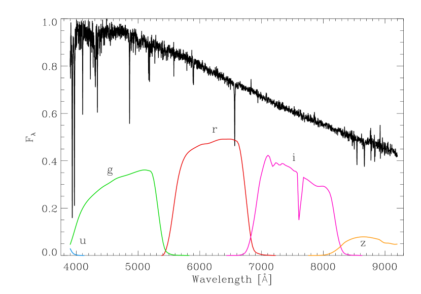
Figure 1: Sample observed spectrum of an F-type star with $[\mathrm{Fe}/\mathrm{H}]\simeq-1.6$, $T_{\mathrm{eff}}\simeq 5886$ K and $\log g\simeq 4.61$. The vertical axis is in flux units normalized to the maximum in the observed spectral region. We also show the total efficiency including atmospheric transmission for the SDSS filter set at 1.3 air masses for point-like objects. Note that filters $u$ and $z$ have contributions outside from the observed spectral region, so that they cannot be used for reconstruction.

In addition to the sparsity condition, the other important ingredient of our technique relies on the election of the sensing matrix. This matrix is the one that relates the underlying spectrum with the measurements we use in the reconstruction. Our aim is to test whether photometric data can be used to reconstruct spectra, so that the sensing matrix is not a choice, but given by the weighting functions of the SDSS filter set. Figure 1 shows the $ugriz$ filter set and an example of an observed spectrum. Note that filters $u$ and $z$ have important contributions outside the observed spectral range. Consequently, the information they contain cannot be easily utilized under the scheme presented in this paper and we carry out the reconstructions using only filters $g$, $r$ and $i$.

Obtaining the magnitude in the filter $k$ of the SDSS system from spectroscopic data reduces to the calculation of the following quantity (Fukugita et al., 1996):

$$m_{k}=-2.5\log_{10}\frac{\int f(\nu)S_{k}(\nu)\mathrm{d}\ln\nu}{\int S_{k}(\nu)\mathrm{d}\ln\nu}-48.6,$$ (4)

where $f(\nu)$ is the flux distribution of the star. Therefore, $S(\nu)$ is the effective transmissivity of the filter, including the filter response, the CCD quantum efficiency and the typical transmission of the sky for a point source (in our cases adopted for an airmass of 1.3). The flux measured for each filter can be estimated using the Riemann integral as (note that more precise quadrature rules can be used without a significant change in the following discussion):

$$\int f(\nu)S_{k}(\nu)\mathrm{d}\ln\nu\approx\sum_{i=1}^{N}S_{k}(\nu_{i})f(\lambda_{i})\frac{\lambda_{i}}{c}\Delta\lambda_{i},$$ (5)

where we have made the integration in the wavelength axis and used $f(\lambda)$ instead of $f(\nu)$ since the principal components of McGurk et al. (2010) are given in terms of $f(\lambda)$. The normalization constant for each filter is obtained likewise:

$$C_{k}=\int S_{k}(\nu)\mathrm{d}\ln\nu\approx\sum_{i=1}^{N}S_{k}(\nu_{i})\frac{\Delta\lambda_{i}}{\lambda_{i}}.$$ (6)

Note that one is able to isolate the flux from the observed magnitudes as:

$$10^{-0.4(m_{k}+48.6)}\approx\frac{1}{C_{k}}\sum_{i=1}^{N}f(\lambda_{i})S_{k}(\nu_{i})\frac{\lambda_{i}}{c}\Delta\lambda_{i}.$$ (7)

Consequently, the flux associated to the measured photometric quantity can be written as the dot product of the original flux distribution $f(\lambda_{i})$ and a weighting function, so that each column of the sensing matrix $\mathbf{\Phi}$ in Eq. (1) is given by:

$$\Phi_{ik}=\frac{S_{k}(\nu_{i})}{C_{k}}\frac{\lambda_{i}}{c}\Delta\lambda_{i}.$$ (8)

2.3 Reconstruction

The sparsity constraint of the spectrum is fulfilled automatically when using a principal component decomposition, with the additional advantage of knowing exactly which coefficients of the sparse vector $\mathbf{a}$ are non-zero. Therefore, the solution of the problem given by Eq. (3) is simpler than the full CS problem in which the non-zero elements of $\mathbf{a}$ have to be identified. Consequently, the solution to Eq. (3) is given by the sparse vector that minimizes the following $\ell_{2}$-norm:

$$\parallel\mathbf{y}-\mathbf{\Phi}\mathbf{W}^{\dagger}\mathbf{a}\parallel_{2}.$$ (9)

In other words, we look for the sparse vector $\mathbf{a}$ with the first $K$ elements different from zero and the rest set to zero that minimizes the square difference between the photometric flux on the $g$, $r$ and $i$ filters and the ones reconstructed using the previous formalism, where the flux is obtained as a linear combination of $K$ principal components. We now develop in more detail the steps to be followed.

Assume that the signal of interest $F(\lambda)$ can be written as a linear combination of $K$ (sparsity) PCA basis functions $B_{i}(\lambda)$, so that:

$$F(\lambda_{i})=\sum_{k=1}^{K}a_{k}B_{k}(\lambda_{i})\qquad\forall i=1,\ldots,M.$$ (10)

The measurement process produces the following linear combinations:

$$y_{j}=\sum_{i=1}^{M}\Phi_{ij}F(\lambda_{i})\qquad\forall j=1,\ldots,N,$$ (11)

where $M$ is the number of wavelength points, $N$ is the number of measurements and the $\Phi_{ij}$ are the matrix elements of the sensing matrix $\mathbf{\Phi}$, given in Eq. (8). Plugging Eq. (10) into Eq. (11), we end up with:

$$y_{j}=\sum_{i=1}^{M}\Phi_{ij}\sum_{k=1}^{K}a_{k}B_{k}(\lambda_{i})=\sum_{k=1}^{K}a_{k}\sum_{i=1}^{M}\Phi_{ij}B_{k}(\lambda_{i}),$$ (12)

where, making the substitution $t_{k}^{j}=\sum_{i=1}^{M}\Phi_{ij}B_{k}(\lambda_{i})$, can be written as:

$$y_{j}=\sum_{k=1}^{K}a_{k}t_{k}^{j}.$$ (13)

The minimization of Eq. (9) can be easily done calculating the derivatives with respect to each $a_{k}$ and equating them to zero. In other words, given the vector $\mathbf{o}$ of length $N$ with the observations (photometry), we define the metric function:

$$\chi^{2}=\sum_{j=1}^{N}\frac{1}{\sigma^{2}_{o_{j}}}\left[o_{j}-\sum_{k=1}^{K}a_{k}t_{k}^{j}\right]^{2},$$ (14)

where $\sigma^{2}_{o_{j}}$ is the variance associated to $o_{j}$ and discussed in §4. Then, we end up with the following set of linear equations for $a_{k}$:

$$\sum_{k=1}^{K}a_{k}\sum_{j=1}^{N}\frac{t_{k}^{j}t_{l}^{j}}{\sigma^{2}_{o_{j}}}=\sum_{j=1}^{N}\frac{o_{j}}{\sigma^{2}_{o_{j}}}t_{l}^{j}\qquad\forall l=1,\ldots,K$$ (15)

In matrix form, we have:

$$\mathbf{G}\mathbf{a}=\mathbf{b},$$ (16)

where

$$G_{kl} = \sum_{j=1}^{N}\frac{t_{k}^{j}t_{l}^{j}}{\sigma^{2}_{o_{j}}}$$

$$b_{l} = \sum_{j=1}^{N}\frac{o_{j}}{\sigma^{2}_{o_{j}}}t_{l}^{j}.$$ (17)

The $t$’s are defined from the principal components of the spectra and the photometric system –they are common for all objects. The only additional information needed for each object is the photometry and its expected uncertainties. Each spectrum is reconstructed by computing the $\mathbf{b}$ vector, calculating $\mathbf{G}^{-1}\mathbf{b}$, and using these numbers in the linear combination of Eq. (10).

It is also of interest to note that the solution to Eq. (9) can alternatively be easily carried out using the SVD of the matrix $\mathbf{\Phi}\mathbf{W}^{\dagger}$. We have verified empirically that this matrix of size $N\times M$ fulfills that $\mathrm{rank}(\mathbf{\Phi}\mathbf{W}^{\dagger})=N$. Thus, in order to reconstruct the spectrum using $N$ principal components, we need to have, at least, $N$ measurements. Since we have only available the $g$, $r$ and $i$ magnitudes, we cannot expect to reconstruct the spectrum using the four principal components tabulated by McGurk et al. (2010) from only 3 measurements. As a consequence, we have to limit the reconstruction to only the average spectrum plus two principal components, leading to slightly larger errors.

Summarizing, from the knowledge of the system response at each wavelength, the principal components associated to the $g-r$ bin of the star and the $g$, $r$, and $i$ magnitudes, one is able to reconstruct the stellar spectrum by solving the linear system of Eq. (16) and using the coefficients in the linear expansion given by Eq. (10).

3 Demonstration of the technique

We carry out reconstructions using magnitudes synthesized from observed spectra included in SDSS Data Release 7. The synthetic magnitudes are obtained following Eq. (4) for filters $g$, $r$ and $i$. These could be taken directly from the photometric observations instead. The sensing matrix is built using Eq. (8). The spectrum of four representative stars from the sample are reconstructed solving the linear system of Eq. (16). The success of the technique is shown in Fig. 2. As stated before, to this aim we make use only of the mean spectrum and two principal components. The original noisy spectrum is shown in black color. The projection of the observed spectrum on the space spanned by the first three principal components is shown in red color. This constitutes the best possible reconstruction that we could achieve with the presented method. The spectrum reconstructed with our technique using the magnitude in the filters $g$, $r$, and $i$ is shown in blue. Note that the reconstruction closely follows the red curve, indicating that a good reconstruction is possible and that the projection along the first three principal components can be obtained reliably from the linear measurements made with the SDSS filters.

The fundamental characteristics of the spectra are reproduced with precision, making it possible to empirically infer spectroscopic quantities using photometric measurements. At the same time, thanks to the projection along the principal components, the spectrum reconstructed from $gri$ magnitudes is automatically denoised (see, e.g., Martínez González et al., 2008, for the denoising capabilities of PCA). Particularly large residuals are visible at specific wavelengths in Fig. 2. In panel a) we can spot some issues with sky removal at the green [OI] line (5577 Å) and in the IR end. In panels b), c) and d) there are strong residuals around the transitions of the Balmer series and other strong features. These residuals change sign very quickly around the central wavelength, signaling a horizontal offset between the original and the reconstructed spectra, most likely related to the Dopper velocity shifts, which have not been corrected but happen to be small enough for the star depicted in panel a).

As four examples are not statistically relevant, we have carried out an analysis of the differences between the reconstructed and original spectra for 5000 stars chosen at random from the seventh data release of the SDSS (Abazajian et al., 2009). We have verified that a sample of this size chosen at random covers all $g-r$ bins and provides reliable statistics. The quality is characterized, at each wavelength, by the 5th, 50th and 95th percentile of the distribution of relative errors from the reconstructed spectrum and the original one. The results are shown in the upper-left panel of Fig. 3. As stated, the 50th percentile (the median) is represented as a black curve and indicates that half of the stars can be reconstructed with relative errors smaller than 2% (from $\sim$4200 to 9000 Å). The 5th and 95th percentiles (blue and red curves) are also indicated in the upper left panel of Fig. 3. It is demonstrated that the reconstructions can be done with relative errors well below 10% for 95% of the stars. Of course, this does not rule out the presence of 5% of the stars with relative reconstruction errors potentially larger than 10%.

For reference, in Fig. 3 reconstructions with the first three (lower left panel) and four (lower right panel) principal components as obtained from McGurk et al. (2010) are compared with the original spectra. These plots summarize the quality of the PCA recreations. Although PCA reconstructions with relative errors below or of the order of 1% are possible for 50% of the stars, a fraction of stellar spectra will incur (even knowing exactly the projections along the principal components) relative errors larger than 10%. Note also that the improvement on the reconstruction is marginal when using four instead of three principal components. An indication of the quality of the PCA reconstruction is that the difference between the initial magnitudes and the reconstructed magnitudes has a standard deviation of 0.008 for $g$, $r$ and $i$ when using 4 principal components. When using only one principal component, this number increases up to 0.03 for $g$ and $r$ and to 0.05 for $i$.

It is important to realize that the residuals shown in Fig. 3 are significantly higher for wavelengths with lines than in continuum regions. This suggests that the PCA reconstruction is reproducing well the continuum shape, but not so the lines’ strength. However, lines are crucial for recovering information on surface gravity and chemical composition. A possibility for improvement is therefore to perform PCA on continuum-corrected spectra.

If instead of using the original spectra as reference, reconstructions are compared with the spectra projected onto the space spanned by the first three principal components, the results are those shown in the upper right panel of Fig. 3. It is clear from this plot that our method is able to reliably extract the projection along the first three principal components from photometric information.

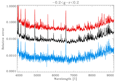
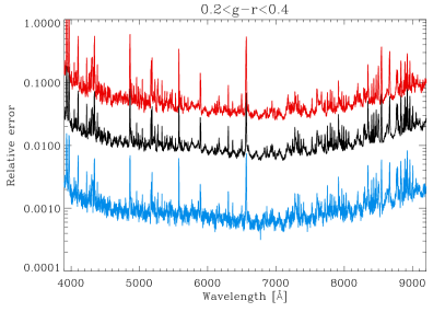
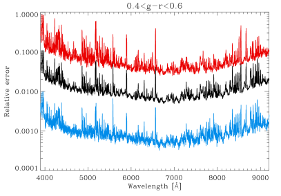
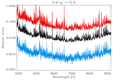
Figure 4: Relative error between the reconstructed spectrum using our method and the original noisy spectrum for the sample separated in color bins. Note that reconstructions of stars with higher effective temperatures (smaller $g-r$) are of better quality due to the small number of spectral features. On the contrary, cooler stars (larger $g-r$) tend to have molecular bands that difficult the reconstruction. In any case, even in the least favourable case, 50% of the stars have relative errors below 4-5% while relative errors are smaller than 20% with 95% probability (with a large wavelength region with errors below 10% for 95% of the stars). The colors have the same meaning as those of Fig. 3.

In order to analyze the quality of reconstructions as a function of the spectral type, we show in Fig. 4 the relative error between the reconstruction and the original noisy spectrum for stars in different bins of $g-r$. As expected, we note that our reconstruction leads to slightly worse results in cooler stars. This is a consequence of the fact that the spectrum of cool stars is relatively more complex and the photometry is not able to capture their full variation. In any case, even in the less favorable case for stars with $g-r>0.6$ ($T_{\mathrm{eff}}\lesssim 5000$ K), reconstructions are below 10% for 95% of the stars in a large wavelength range.

4 Influence of errors

Observed magnitudes are always inherently accompanied by an error bar. It is important to quantify the effect of this error on the reconstruction of the spectrum. Assuming Gaussian errors, an error bar of standard deviation $\sigma_{m_{j}}$ in magnitudes at filter $j$ translates into an error bar in the flux at the same filter of:

$$\sigma_{o_{j}}=0.4\ln 10o_{j}\sigma_{m_{j}}\approx 0.92o_{j}\sigma_{m_{j}}.$$ (18)

Even if we assume that the error bars of the observations are not correlated, the resulting error bars for the projections along the mean spectrum and the principal components are correlated. Assuming that the matrix $\mathbf{G}$ is noise-free, error propagation in the solution of the linear system of Eq. (16) leads to the following formula for the covariance matrix of the projection along the principal components:

$$\mathbf{C}_{a}=\mathbf{G}^{-1}\mathbf{C}_{b}(\mathbf{G}^{-1})^{\dagger},$$ (19)

where

$$\mathbf{C}_{b}=\mathbf{T}\mathbf{C}_{o}\mathbf{T}^{\dagger},$$ (20)

where $T_{ij}=t_{i}^{j}/\sigma^{2}_{o_{j}}$. For simplicity, we assume that the correlation matrix of the observed fluxes is diagonal and the diagonal elements are computed from Eq. (18). Finally, the covariance matrix for the reconstructed spectrum is given by:

$$\mathbf{C}_{F}=\mathbf{W}^{\dagger}\mathbf{C}_{a}\mathbf{W}.$$ (21)

It is difficult to characterize the sensitivity to errors in the observed magnitudes because of the large variability in the stellar fluxes. For presentation purposes and to give a rough estimation, let us assume that all Sloan magnitudes have $\sigma_{m}=0.03$ mag, which is representative of more than 95% of the observed stars. Likewise, let us pick a representative value for the flux at each filter $o_{j}$ as the average in each bin. Following the previous expressions, we show in Figure 5 the standard deviation of the error in the projection along the principal components (equivalent to the diagonal elements $\mathrm{cov}(a_{i},a_{i})$) normalized to the product of the observational error in the magnitude and the mean projection along the mean spectrum. It has been estimated for the average flux in each bin. The results indicate that the relative error in the projection along the principal components is roughly similar to $\sigma_{m}$. In the SDSS database, typical errors range from 0.01 to 0.05 mag, with more than 95% of the stars with errors less than 0.03 mag. Therefore, relative errors of 1-3% are induced in the reconstruction due to the presence of uncertainties in the observed magnitudes.

The principal components of McGurk et al. (2010) have been computed by shifting all spectra to a zero radial velocity common wavelength axis. Therefore, the reconstructions we carry out give as an output the spectrum at zero radial velocity and contain no information on radial velocities. However, the fluxes measured photometrically with the $gri$ filters contain the influence of the radial velocity. This effect cannot be compensated for and it is not clear whether this might have an influence on the final reconstruction. From SDSS data, the distribution of radial velocities induce Doppler shifts that are, with $\sim$95% probability, smaller than 6 pixels ($\sim$414 km/s). According to the reconstructions shown in Figs. 2 and 3, that were performed with the original spectrum, Doppler shifts increase errors in the lines, as suggested by the antisymmetric residuals in the strongest lines of panels b) c) and d) in Fig. 2 Such errors are masked in Fig. 3 by the symmetrization induced by averaging out over many stars. Therefore, although radial velocities cannot be estimated with our method, its effect on the quality of the reconstruction is not very important, except for spectral lines.

5 Conclusions

We have presented a method to reconstruct stellar spectra from SDSS photometry that is fast, efficient and reliable. Although it might sound magical, this reconstruction is made possible thanks to the sparsity of stellar spectra, which can be expressed as a linear combination of a few eigenspectra obtained from a principal component decomposition. Our method returns the projection of the observed spectrum onto the space spanned by the first three principal components just from the photometric $g$, $r$ and $i$ magnitudes. As a consequence, the resulting spectrum is simultaneously denoised and reconstructed. We have analyzed the statistical properties of the regenerated spectra and verified that the residuals are roughly compatible with the noise present in the observations, albeit they are not random. We have also analyzed the influence of observational errors in the magnitudes and the presence of non-zero radial velocities on the reconstruction. Both of them produce very small effects on the performance of our algorithm.

Recently, McGurk et al. (2010) has investigated the possible correlation between stellar parameters and the projections of the spectrum along the principal components. Since PCA is a linear technique and the stellar parameters are typically nonlinear combinations of parts of the observed spectrum, a strong correlation is not to be expected, as shown by McGurk et al. (2010). In our case though, we are able to reconstruct the full spectrum from photometric observables. This opens up the possibility of applying standard techniques for inferring stellar parameters to the reconstructed spectrum.

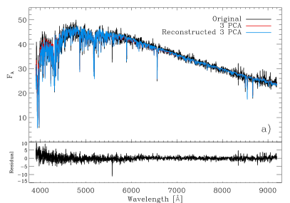
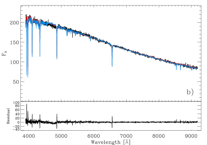
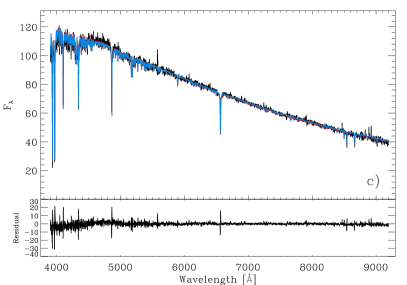
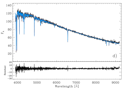
Figure 2: Four examples of the spectrum reconstruction using simulated magnitudes in filters $g$, $r$ and $i$. The original spectrum is shown in black. The spectrum reconstructed from the exact projections along the first 3 principal components of McGurk et al. (2010) is shown in red. This constitutes the best reconstruction of the spectrum we can achieve with our method. The spectrum reconstructed using our scheme is shown in blue, with the residual indicated in the lower subpanel of each panel. Note the similarity between the red and blue curves.

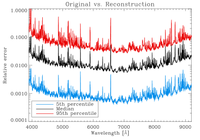
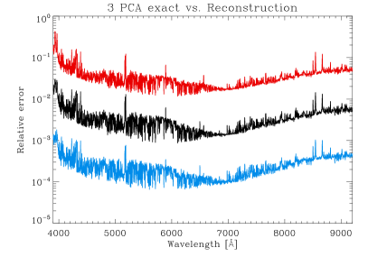
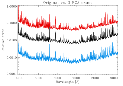
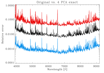
Figure 3: Statistical comparison showing the viability of the reconstruction scheme for 5000 stars chosen at random from the database of McGurk et al. (2010). We show the 5th (blue curve), 50th (black curve) and 95th (red curve) percentiles of the relative error distribution for each wavelength. The upper left panel presents the relative error obtained between the reconstructed spectrum using our method and the original noisy spectrum. It is clear that 50% of the stars have relative errors below 1-2% while relative errors are smaller than 10% with 95% probability. The upper right panel shows the relative error between the reconstruction using photometric data and the denoised spectrum computed with the exact projections along the first three principal components. For reference, the lower panels show the comparison between the original spectra and the ones reconstructed using the exact projections along the first three (lower left panel) and the first four (lower right panel) principal components.

Figure 5: Standard deviation of the error in the reconstruction of the projection of the spectrum along the mean spectrum and the first two principal components for each bin. The color $g-r$ for each bin is also indicated in the upper axis. The error is normalized to the quantity $\sigma_{m}$ and estimated using the average flux in each filter for each bin.

References

- Abazajian et al. (2009) Abazajian, K. N., et al. 2009, ApJS, 182, 543
- Asensio Ramos (2010) Asensio Ramos. 2010, Astron. Nachr., in press
- Asensio Ramos & Collados (2008) Asensio Ramos, A., & Collados, M. 2008, Appl. Opt., 47, 2541
- Asensio Ramos & López Ariste (2010) Asensio Ramos, A., & López Ariste, A. 2010, A&A, 509, A49+
- Bessell (2005) Bessell, M. S. 2005, ARA&A, 43, 293
- Candès et al. (2006) Candès, E., Romberg, J., & Tao, T. 2006, Comm. Pure Appl. Math., 59, 1207
- Cepa et al. (2000) Cepa, J., et al. 2000, in Presented at the Society of Photo-Optical Instrumentation Engineers (SPIE) Conference, Vol. 4008, Society of Photo-Optical Instrumentation Engineers (SPIE) Conference Series, ed. M. Iye & A. F. Moorwood, 623–631
- Connolly et al. (1995) Connolly, A. J., Szalay, A. S., Bershady, M. A., Kinney, A. L., & Calzetti, D. 1995, AJ, 110, 1071
- Donoho (2006) Donoho, D. 2006, IEEE Trans. on Information Theory, 52, 1289
- Fukugita et al. (1996) Fukugita, M., Ichikawa, T., Gunn, J. E., Doi, M., Shimasaku, K., & Schneider, D. P. 1996, AJ, 111, 1748
- Ivezić et al. (2008) Ivezić, Ž., et al. 2008, ApJ, 684, 287
- Ivezić et al. (2005) Ivezić, Ž., Vivas, A. K., Lupton, R. H., & Zinn, R. 2005, AJ, 129, 1096
- Karhunen (1947) Karhunen, K. 1947, Ann. Acad. Sci. Fennicae. Ser. A. I. Math.-Phys., 37, 1
- Loève (1955) Loève, M. M. 1955, Probability Theory (Princeton: Van Nostrand Company)
- Martínez González et al. (2008) Martínez González, M. J., Asensio Ramos, A., Carroll, T. A., Kopf, M., Ramírez Vélez, J. C., & Semel, M. 2008, A&A, 486, 637
- McGurk et al. (2010) McGurk, R. C., Kimball, A. E., & Ivezic, Z. 2010, ArXiv e-prints
- Pearson (1901) Pearson, K. 1901, Philosophical Magazine, 2, 559
- Press et al. (1986) Press, W. H., Teukolsky, S. A., Vetterling, W. T., & Flannery, B. P. 1986, Numerical Recipes (Cambridge: Cambridge University Press)
- Skrutskie et al. (2006) Skrutskie, M. F., et al. 2006, AJ, 131, 1163
- Strömgren (1951) Strömgren, B. 1951, AJ, 56, 142
- Strömgren (1956) —. 1956, Vistas in Astronomy, 2, 1336
- Yip et al. (2004) Yip, C. W., Connolly, A. J., Vanden Berk, D. E., Ma, Z., Frieman, J. A., SubbaRao, M., Szalay, A. S., Richards, G. T., Hall, P. B., Schneider, D. P., Hopkins, A. M., Trump, J., & Brinkmann, J. 2004, AJ, 128, 2603