Resource Allocation using Virtual Clusters

Abstract

In this report we demonstrate the potential utility of resource allocation management systems that use virtual machine technology for sharing parallel computing resources among competing jobs. We formalize the resource allocation problem with a number of underlying assumptions, determine its complexity, propose several heuristic algorithms to find near-optimal solutions, and evaluate these algorithms in simulation. We find that among our algorithms one is very efficient and also leads to the best resource allocations. We then describe how our approach can be made more general by removing several of the underlying assumptions.

1 Introduction

The use of commodity clusters has become mainstream for high-performance computing applications, with more than 80% of today’s fastest supercomputers being clusters [49]. Large-scale data processing [23, 39, 33] and service hosting [22, 4] are also common applications. These clusters represent significant equipment and infrastructure investment, and having a high rate of utilization is key for justifying their ongoing costs (hardware, power, cooling, staff) [24, 50]. There is therefore a strong incentive to share these clusters among a large number of applications and users.

The sharing of compute resources among competing instances of applications, or jobs, within a single system has been supported by operating systems for decades via time-sharing. Time-sharing is implemented with rapid context-switching and is motivated by a need for interactivity. A fundamental assumption is that there is no or little a-priori knowledge regarding the expected workload, including expected durations of running processes. This is very different from the current way in which clusters are shared. Typically, users request some fraction of a cluster for a specified duration. In the traditional high-performance computing arena, the ubiquitous approach is to use “batch scheduling”, by which jobs are placed in queues waiting to gain exclusive access to a subset of the platform for a bounded amount of time. In service hosting or cloud environments, the approach is to allow users to lease “virtual slices” of physical resources, enabled by virtual machine technology. The latter approach has several advantages, including O/S customization and interactive execution. In general resource sharing among competing jobs is difficult because jobs have different resource requirements (amount of resources, time needed) and because the system cannot accommodate all jobs at once.

An important observation is that both resource allocation approaches mentioned above dole out integral subsets of the resources, or allocations (e.g., 10 physical nodes, 20 virtual slices), to jobs. Furthermore, in the case of batch scheduling, these subsets cannot change throughout application execution. This is a problem because most applications do not use all resources allocated to them at all times. It would then be useful to be able to decrease and increase application allocations on-the-fly (e.g., by removing and adding more physical cluster nodes or virtual slices during execution). Such application are termed “malleable” in the literature. While solutions have been studied to implement and to schedule malleable applications [46, 12, 25, 51, 52], it is often difficult to make sensible malleability decisions at the application level. Furthermore, many applications are used as-is, with no desire or possibility to re-engineer them to be malleable. As a result sensible and automated malleability is rare in real-world applications. This is perhaps also due to the fact that production batch scheduling environments do not provide mechanisms for dynamically increasing or decreasing allocations. By contrast, in service hosting or cloud environments, acquiring and relinquishing virtual slices is straightforward and can be implemented via simple mechanisms. This provides added motivation to engineer applications to be malleable in those environments.

Regardless, an application that uses only 80% of a cluster node or of a virtual slice would need to relinquish only 20% of this resources. However, current resource allocation schemes allocate integral numbers of resources (whether these are physical cluster nodes or virtual slices). Consequently, many applications are denied access to resources, or delayed, in spite of cluster resources not being fully utilized by the applications that are currently executing, which hinders both application throughput and cluster utilization.

The second limitation of current resource allocation schemes stems from the fact that resource allocation with integral allocations is difficult from a theoretical perspective [10]. Resource allocation problems are defined formally as the optimizations of well-defined objective functions. Due to the difficulty (i.e., NP-hardness) of resource allocation for optimizing an objective function, in the real-world no such objective function is optimized. For instance, batch schedulers instead provide a myriad of configuration parameters by which a cluster administrator can tune the scheduling behavior according to ad-hoc rules of thumb. As a result, it has been noted that there is a sharp disconnect between the desires of users (low application turn-around time, fairness) and the schedules computed by batch schedulers [44, 26]. It turns out that cluster administrators often attempt to maximize cluster utilization. But recall that, paradoxically, current resource allocation schemes inherently hinder cluster utilization!

A notable finding in the theoretical literature is that with job preemption and/or migration there is more flexibility for resource allocation. In this case certain resource allocation problems become (more) tractable or approximable [6, 44, 27, 35, 11]. Unfortunately, preemption and migration are rarely used on production parallel platforms. The gang scheduling [38] approach allows entire parallel jobs to be context-switched in a synchronous fashion. Unfortunately, a known problem with this approach is the overhead of coordinated context switching on a parallel platform. Another problem is the memory pressure due to the fact that cluster applications often use large amounts of memory, thus leading to costly swapping between memory and disk [9]. Therefore, while flexibility in resource allocations is desirable for solving resource allocation problems, affording this flexibility has not been successfully accomplished in production systems.

In this paper we argue that both limitations of current resource allocation schemes, namely, reduced utilization and lack of an objective function, can be addressed simultaneously via fractional and dynamic resource allocations enabled by state-of-the-art virtual machine (VM) technology. Indeed, applications running in VM instances can be monitored so as to discover their resource needs, and their resource allocations can be modified dynamically (by appropriately throttling resource consumption and/or by migrating VM instances). Furthermore, recent VM technology advances make the above possible with low overhead. Therefore, it is possible to use this technology for resource allocation based on the optimization of sensible objective functions, e.g., ones that capture notions of performance and fairness.

Our contributions are:

• We formalize a general resource allocation problem based on a number of assumptions regarding the platform, the workload, and the underlying VM technology;

• We establish the complexity of the problem and propose algorithms to solve it;

• We evaluate our proposed algorithms in simulation and identify an algorithm that is very efficient and leads to better resource allocations than its competitors;

• We validate our assumptions regarding the capabilities of VM technology;

• We discuss how some of our other assumptions can be removed and our approach adapted to parallel jobs and dynamic jobs.

This paper is organized as follows. In Section 2 we define and formalize our target problem, we list our assumptions for the base problem, and we establish its NP-hardness. In Section 3 we propose algorithms for solving the base problem and evaluate these algorithms in simulation in Section 4. Sections 5 and 6 study the resource sharing problem with relaxed assumptions regarding the nature of the workload, thereby handling parallel and dynamic workloads. In Section 7 we validate our fundamental assumption that VM technology allows for precise resource sharing. Section 8 discusses related work. Section 9 discusses future directions. Finally, Section 10 concludes the paper with a summary of our findings.

2 Flexible Resource Allocation

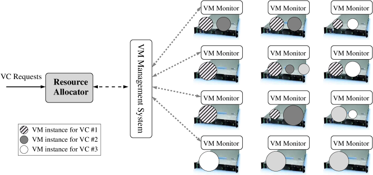
Figure 1: System architecture with 12 homogeneous physical hosts and 3 running virtual clusters.

2.1 Overview

In this work we consider a homogeneous cluster platform, which is managed by a resource allocation system. The architecture of this system is depicted in Figure 1. Users submit job requests, and the system responds by creating sets of VM instances, or “virtual clusters” (VC) to run the jobs. These instances run on physical hosts that are each under the control of a VM monitor [8, 53, 34]. The VM monitor can enforce specific resource consumption rates for different VMs running on the host. All VM monitors are under the control of a VM management system that can specify resource consumption rates for VM instances running on the physical cluster. Furthermore, the VM resource management system can enact VM instance migrations among physical hosts. An example of such a system is the Usher project [32]. Finally, a Resource Allocator (RA) makes decisions regarding whether a request for a VC should be rejected or admitted, regarding possible VM migrations, and regarding resource consumption rates for each VM instance.

Our overall goal is to design algorithms implemented as part of the RA that make all virtual clusters “play nice” by allowing fine-grain tuning of their resource consumptions. The use of VM technology is key for increasing cluster utilization, as it makes is possible to allocate to VCs only the resources they need when they need them. The mechanisms for allowing on-the-fly modification of resource allocations are implemented as part of the VM Monitors and the VM Management System.

A difficult question is how to define precisely what “playing nice” means, as it should encompass both notions of individual job performance and notions of fairness among jobs. We address this issue by defining a performance metric that encompasses both these notions and that can be used to value resource allocations. The RA may be configured with the goal of optimizing this metric but at the same time ensuring that the metric across the jobs is above some threshold (for instance by rejecting requests for new virtual clusters). More generally, a key aspect of our approach is that it can be combined with resource management and accounting techniques. For instance, it is straightforward to add notions of user priorities, of resource allocation quotas, of resource allocation guarantees, or of coordinated resource allocations to VMs belonging to the same VC. Furthermore, the RA can reject or delay VC requests if the performance metric is below some acceptable level, to be defined by cluster administrators.

2.2 Assumptions

We first consider the resource sharing problem using the following six assumptions regarding the workload, the physical platform, and the VM technology in use:

(H1)

Jobs are CPU-bound and require a given amount of memory to be able to run;

(H2)

Job computational power needs and memory requirements are known;

(H3)

Each job requires only one VM instance;

(H4)

The workload is static, meaning jobs have constant resource requirements; furthermore, no job enters or leaves the system;

(H5)

VM technology allows for precise, low-overhead, and quickly adaptable sharing of the computational capabilities of a host across CPU-bound VM instances.

These assumptions are very stringent, but provide a good framework to formalize our resource allocation problem (and to prove that it is difficult even with these assumptions). We relax assumption H3 in Section 5, that is, we consider parallel jobs. Assumption H4 amounts to assuming that jobs have no time horizons, i.e., that they run forever with unchanging requirements. In practice, the resource allocation may need to be modified when the workload changes (e.g., when a new job arrives, when a job terminates, when a job starts needing more/fewer resources). In Section 6 we relax assumption H4 and extend our approach to allow allocation adaptation. We validate assumption H5 in Section 7. We leave relaxing H1 and H2 for future work, and discuss the involved challenges in Section 10.

2.3 Problem Statement

We call the resource allocation problem described in the previous section VCSched and define it here formally. Consider $H>0$ identical physical hosts and $J>0$ jobs. For job $i$, $i=1,\ldots,J$, let $\alpha_{i}$ be the (average) fraction of a host’s computational capability utilized by the job if alone on a physical host, $0\leq\alpha_{i}\leq 1$. (Alternatively, this fraction could be specified a-priori by the user who submitted/launched job $i$.) Let $m_{i}$ be the maximum fraction of a host’s memory needed by job $i$, $0\leq m_{i}\leq 1$. Let $\alpha_{ij}$ be the fraction of the computational capability of host $j$, $j=1,\ldots,H$, allocated to job $i$, $i=1,\ldots,J$. We have $0\leq\alpha_{ij}\leq 1$. If $\alpha_{ij}$ is constrained to be an integer, that is either $0$ or $1$, then the model is that of scheduling with exclusive access to resources. If, instead, $\alpha_{ij}$ is allowed to take rational values between $0$ and $1$, then resource allocations can be fractional and thus more fine-grain.

Constraints –

We can write a few constraints due to resource limitations. We have

$$\forall j\quad\sum_{i=1}^{J}\alpha_{ij}\leq 1\;,$$

which expresses the fact that the total CPU fraction allocated to jobs on any single host may not exceed 100%. Also, a job should not be allocated more resource than it can use:

$$\forall i\quad\sum_{j=1}^{H}\alpha_{ij}\leq\alpha_{i}\;,$$

Similarly,

$$\forall j\quad\sum_{i=1}^{J}\lceil\alpha_{ij}\rceil m_{i}\leq 1\;,$$ (1)

since at most the entire memory on a host may be used.

With assumption H3, a job requires only one VM instance. Furthermore, as justified hereafter, we assume that we do not use migration and that a job can be allocated to a single host. Therefore, we write the following constraints:

$$\forall i\quad\sum_{j=1}^{H}\lceil\alpha_{ij}\rceil=1\;,$$ (2)

which state that for all $i$ only one of the $\alpha_{ij}$ values is non-zero.

Objective function –

We wish to optimize a performance metric that encompasses both notions of performance and of fairness, in an attempt at designing the scheduler from the start with a user-centric metric in mind (unlike, for instance, current batch schedulers). In the traditional parallel job scheduling literature, the metric commonly acknowledged as being a good measure for both performance and fairness is the stretch (also called “slowdown”) [10, 16]. The stretch of a job is defined as the job’s turn-around time divided by the turn-around time that would have been achieved had the job been alone in the system.

This metric cannot be applied directly in our context because jobs have no time horizons. So, instead, we use a new metric, which we call the yield and which we define for job $i$ as $\sum_{j}\alpha_{ij}/\alpha_{i}$. The yield of a job represents the fraction of its maximum achievable compute rate that is achieved (recall that for each $i$ only one of the $\alpha_{ij}$ is non-zero). A yield of $1$ means that the job consumes compute resources at its peak rate. We can now define problem VCSched as maximizing the minimum yield in an attempt at optimizing both performance and fairness (similar in spirit to minimizing the maximum stretch [10, 27]). Note that we could easily maximize the average yield instead, but we may then decrease the fairness of the resource allocation across jobs as average metrics are starvation-prone [27]. Our approach is agnostic to the particular objective function (although some of our results hold only for linear objective functions). For instance, other ways in which the stretch can be optimized have been proposed [7] and could be adapted for our yield metric.

Migration –

The formulation of our problem precludes the use of migration. However, as when optimizing job stretch, migration could be used to achieve better results. Indeed, assuming that migration can be done with no overhead or cost whatsoever, migrating tasks among hosts in a periodic steady-state schedule afford more flexibility for resource sharing, which could in turn be used to maximize the minimum yield further. For instance, consider 2 hosts and 3 tasks, with $\alpha_{1}=\alpha_{2}=\alpha_{3}=0.6$. Without migration the optimal minimum yield is $0.5/0.6\sim.83$ (which corresponds to an allocation in which two tasks are on the same host and each receive 50% of that host’s computing power). With migration it is possible to do better. Consider a periodic schedule that switches between two allocations, so that on average the schedule uses each allocation 50% of the time. In the first allocation tasks $1$ and $2$ share the first host, each receiving 45% and 55% of the host’s computing power, respectively, and task $3$ is on the second host by itself, thus receiving 60% of its compute power. In the second allocation, the situation is reversed, with task 1 by itself on the first host and task 2 and 3 on the second host, task 2 receiving 55% and task 3 receiving 45%. With this periodic schedule, the average yield of task 1 and 3 is $.5\times(.45/.60+.60/.60)\sim.87$ , and the average yield of task 2 is $.55/.60\sim.91$. Therefore the minimum yield is $.87$, which is higher than that in the no-migration case.

Unfortunately, the assumption that migration comes at no cost or overhead is not realistic. While recent advances in VM migration technology [13] make it possible for a VM instance to change host with a nearly imperceptible delay, migration consumes network resources. It is not clear whether the pay-off of these extra migrations would justify the added cost. It could be interesting to allow a bounded number of migrations for the purpose of further increasing minimum yield, but for now we leave this question for future work. We use migration only for the purpose of adapting to dynamic workloads (see Section 6).

2.4 Complexity Analysis

Let us consider the decision problem associated to VCSched: Is it possible to find an allocation so that its minimum yield is above a given bound, $K$? We term this problem VCSched-Dec. Not surprisingly, VCSched-Dec is NP-complete. For instance, considering only job memory constraints and two hosts, the problem trivially reduces to 2-Partition, which is known to be NP-complete in the weak sense [18]. We can actually prove a stronger result:

Theorem 1.

VCSched-Dec is NP-complete in the strong sense even if host memory capacities are infinite.

Proof.

VCSched-Dec belongs to NP because a solution can easily be checked in polynomial time. To prove NP-completeness, we use a straightforward reduction from 3-Partition, which is known to be NP-complete in the strong sense [18]. Let us consider, $\mathcal{I}_{1}$, an arbitrary instance of 3-Partition: given $3n$ positive integers $\{a_{1},\ldots,a_{3n}\}$ and a bound $R$, assuming that $\frac{R}{4}<a_{i}<\frac{R}{2}$ for all $i$ and that $\sum_{i=j}^{3n}a_{j}=nR$, is there a partition of these numbers into $n$ disjoint subsets $I_{1},\ldots,I_{n}$ such that $\sum_{j\in I_{i}}a_{j}=R$ for all $i$? (Note that $|I_{i}|=3$ for all $i$.) We now build $\mathcal{I}_{2}$, an instance of VCSched as follows. We consider $H=n$ hosts and $J=3n$ jobs. For job $j$ we set $\alpha_{j}=a_{j}/R$ and $m_{j}=0$. Setting $m_{j}$ to $0$ amounts to assuming that there is no memory contention whatsoever, or that host memories are infinite. Finally, we set $K$, the bound on the yield, to be $1$. We now prove that $\mathcal{I}_{1}$ has a solution if and only if $\mathcal{I}_{2}$ has a solution.

Let us assume that $\mathcal{I}_{1}$ has a solution. For each job $j$, we assign it to host $i$ if $j\in I_{i}$, and we give it all the compute power it needs ($\alpha_{ji}=a_{j}/R$). This is possible because $\sum_{j\in I_{i}}a_{j}=R$, which implies that $\sum_{j\in I_{i}}\alpha_{ji}=R/R\leq 1$. In other terms, the computational capacity of each host is not exceeded. As a result, each job has a yield of $K=1$ and we have built a solution to $\mathcal{I}_{2}$.

Let us now assume that $\mathcal{I}_{2}$ has a solution. Then, for each job $j$ there exists a unique $i_{j}$ such that $\alpha_{ji_{j}}=\alpha_{j}$, and such that $\alpha_{ji}=0$ for $i\neq i_{j}$ (i.e., job $j$ is allocated to host $i_{j}$). Let us define $I_{i}=\{j|i_{j}=i\}$. By this definition, the $I_{i}$ sets are disjoint and form a partition of $\{1,\ldots,3n\}$.

To ensure that each processor’s compute capability is not exceeded, we must have $\sum_{j\in I_{i}}\alpha_{j}\leq 1$ for all $i$. However, by construction of $\mathcal{I}_{2}$, $\sum_{j=1}^{3n}\alpha_{j}=n$. Therefore, since the $I_{i}$ sets form a partition of $\{1,\ldots,3n\}$, $\sum_{j\in I_{i}}\alpha_{j}$ is exactly equal to 1 for all $i$. Indeed, if $\sum_{j\in I_{i_{1}}}\alpha_{j}$ were strictly lower than $1$ for some $i_{1}$, then $\sum_{j\in I_{i_{2}}}\alpha_{j}$ would have to be greater than $1$ for some $i_{2}$, meaning that the computational capability of a host would be exceeded. Since $\alpha_{j}=a_{j}/R$, we obtain $\sum_{j\in I_{i}}a_{j}=R$ for all $i$. Sets $I_{i}$ are thus a solution to $\mathcal{I}_{1}$, which concludes the proof.

∎

2.5 Mixed-Integer Linear Program Formulation

It turns out that VCSched can be formulated as a mixed-integer linear program (MILP), that is an optimization problem with linear constraints and objective function, but with both rational and integer variables. Among the constraints given in Section 2.3, the constraints in Eq. 1 and Eq. 2 are non-linear. These constraints can easily be made linear by introducing a binary integer variables, $e_{ij}$, set to 1 if job $i$ is allocated to resource $j$, and to 0 otherwise. We can then rewrite the constraints in Section 2.3 as follows, with $i=1,\ldots,J$ and $j=1,\ldots,H$:

$$\forall i,j \quad e_{ij}\in\mathbb{N},$$ (3)

$$\forall i,j \quad\alpha_{ij}\in\mathbb{Q},$$ (4)

$$\forall i,j 0\leq e_{ij}\leq 1,$$ (5)

$$\forall i,j 0\leq\alpha_{ij}\leq e_{ij},$$ (6)

$$\forall i \sum_{j=1}^{H}e_{ij}=1,$$ (7)

$$\forall j \sum_{i=1}^{J}\alpha_{ij}\leq 1,$$ (8)

$$\forall j \sum_{i=1}^{J}e_{ij}m_{i}\leq 1\;$$ (9)

$$\forall i \sum_{j=1}^{H}\alpha_{ij}\leq\alpha_{i}\;$$ (10)

$$\forall i \sum_{j=1}^{H}\frac{\alpha_{ij}}{\alpha_{i}}\geq Y$$ (11)

Recall that $m_{i}$ and $\alpha_{i}$ are constants that define the jobs. The objective is to maximize $Y$, i.e., to maximize the minimum yield.

3 Algorithms for Solving VCSched

In this section we propose algorithms to solve VCSched, including exact and relaxed solutions of the MILP in Section 2.5 as well as ad-hoc heuristics. We also give a generally applicable technique to improve average yield further once the minimum yield has been maximized.

3.1 Exact and Relaxed Solutions

In general, solving a MILP requires exponential time and is only feasible for small problem instances. We use a publicly available MILP solver, the Gnu Linear Programming Toolkit (GLPK), to compute the exact solution when the problem instance is small (i.e., few tasks and/or few hosts). We can also solve a relaxation of the MILP by assuming that all variables are rational, converting the problem to a LP. In practice a rational linear program can be solved in polynomial time. However, the resulting solution may be infeasible (namely because it could spread a single job over multiple hosts due to non-binary $e_{ij}$ values), but has two important uses. First, the value of the objective function is an upper bound on what is achievable in practice, which is useful to evaluate the absolute performance of heuristics. Second, the rational solution may point the way toward a good feasible solution that is computed by rounding off the $e_{ij}$ values to integer values judiciously, as discussed in the next section.

It turns out that we do not need a linear program solver to compute the optimal minimum yield for the relaxed program. Indeed, if the total of job memory requirement is not larger than the total available memory (i.e., if $\sum_{i=1}^{J}m_{i}\leq H$), then there is a solution to the relaxed version of the problem and the achieved optimal minimum yield, $Y^{(\text{rat})}_{\text{opt}}$, can be computed easily:

$$Y^{(\text{rat})}_{\text{opt}}=min\{\frac{H}{\sum_{i=1}^{J}\alpha_{i}},1\}.$$

The above expression is an obvious upper bound on the maximum minimum yield. To show that it is in fact the optimal, we simply need to exhibit an allocation that achieves this objective. A simple such allocation is:

$$\forall i,j\hskip 7.22743pte_{ij}=\frac{1}{H}\hskip 7.22743pt\text{and}\hskip 7.22743pt\alpha_{ij}=\frac{1}{H}\alpha_{i}Y^{(\text{rat})}_{\text{opt}}.$$

3.2 Algorithms Based on Relaxed Solutions

We propose two heuristics, RRND and RRNZ, that use a solution of the rational LP as a basis and then round-off rational $e_{ij}$ value to attempt to produce a feasible solution, which is a classical technique. In the previous section we have shown a solution for the LP; Unfortunately, that solution has the undesirable property that it splits each job evenly across all hosts, meaning that all $e_{ij}$ values are identical. Therefore it is a poor starting point for heuristics that attempt to round off $e_{ij}$ values based on their magnitude. Therefore, we use GLPK to solve the relaxed MILP and use the produced solution as a starting point instead.

Randomized Rounding (RRND) – This heuristic first solves the LP. Then, for each job $i$ (taken in an arbitrary order), it allocates it to a random host using a probability distribution by which host $j$ has probability $e_{ij}$ of being selected. If the job cannot fit on the selected host because of memory constraints, then that host’s probability of being selected is set to zero and another attempt is made with the relative probabilities of the remaining hosts adjusted accordingly. If no selection has been made and every host has zero probability of being selected, then the heuristic fails. Such a probabilistic approach for rounding rational variable values into integer values has been used successfully in previous work [31].

Randomized Rounding with No Zero probability (RRNZ) – This heuristic is a slight modification of the RRND heuristic. One problem with RRND is that a job, $i$, may not fit (in terms of memory requirements) on any of the hosts, $j$, for which $e_{ij}>0$, in which case the heuristic would fail to generate a solution. To remedy this problem, we set each $e_{ij}$ value equal to zero in the solution of the relaxed MILP to $\epsilon$ instead, where $\epsilon<<1$ (we used $\epsilon=0.01$). For those problem instances for which RRND provides a solution RRNZ should provide nearly the same solution most of the time. But RRNZ should also provide a solution to a some instances for which RRND fails, thus achieving a better success rate.

3.3 Greedy Algorithms

Greedy (GR) – This heuristic first goes through the list of jobs in arbitrary order. For each job the heuristic ranks the hosts according to their total computational load, that is, the total of the maximum computation requirements of all jobs already assigned to a host. The heuristic then selects the first host, in non-decreasing order of computational load, for which an assignment of the current job to that host will satisfy the job’s memory requirements.

Sorted-Task Greedy (SG) – This version of the greedy heuristic first sorts the jobs in descending order by their memory requirements before proceeding as in the standard greedy algorithm. The idea is to place relatively large jobs while the system is still lightly loaded.

Greedy with Backtracking (GB) – It is possible to modify the GR heuristic to add backtracking. Clearly full-fledged backtracking would lead to 100% success rate for all instances that have a feasible solution, but it would also require potentially exponential time. One thus needs methods to prune the search tree. We use a simple method, placing an arbitrary bound (500,000) on the number of job placement attempts. An alternate pruning technique would be to restrict placement attempts to the top 25% candidate placements, but based on our experiments it is vastly inferior to using an arbitrary bound on job placement attempts.

Sorted Greedy with Backtracking (SGB) – This version is a combination of SG and GB, i.e., tasks are sorted in descending order of memory requirement as in SG and backtracking is used as in GB.

3.4 Multi-Capacity Bin Packing Algorithms

Resource allocation problems are often akin to bin packing problems, and VCSched is no exception. There are however two important differences between our problem and bin packing. First, our tasks resource requirements are dual, with both memory and CPU requirements. Second, our CPU requirements are not fixed but depend on the achieved yield. The first difference can be addressed by using “multi-capacity” bin packing heuristics. Two Multi-capacity bin packing heuristics were proposed in [28] for the general case of $d$-capacity bins and items, but in the $d=2$ case these two algorithms turn out to be equivalent. The second difference can be addressed via a binary search on the yield value.

Consider an instance of VCSched and a fixed value of the yield, $Y$, that needs to be achieved. By fixing $Y$, each task has both a fixed memory requirement and a fixed CPU requirement, both taking values between 0 and 1, making it possible to apply the algorithm in [28] directly.

Accordingly, one splits the tasks into two lists, with one list containing the tasks with higher CPU requirements than memory requirements and the other containing the tasks with higher memory requirements than CPU requirements. One then sorts each list. In [28] the lists are sorted according to the sum of the CPU and memory requirements.

Once the lists are sorted, one can start assigning tasks to the first host. Lists are always scanned in order, searching for a task that can “fit” on the host, which for the sake of this discussion we term a “possible task”. Initially one searches for a possible task in one and then the other list, starting arbitrarily with any list. This task is then assigned to the host. Subsequently, one always searches for a possible task from the list that goes against the current imbalance. For instance, say that the host’s available memory capacity is 50% and its available CPU capacity is 80%, based on tasks that have been assigned to it so far. In this case one would scan the list of tasks that have higher CPU requirements than memory requirements to find a possible task. If no such possible task is found, then one scans the other list to find a possible task. When no possible tasks are found in either list, one starts this process again for the second host, and so on for all hosts. If all tasks can be assigned in this manner on the available hosts, then resource allocation is successful. Otherwise resource allocation fails.

The final yield must be between $0$, representing failure, and the smaller of $1$ or the total computation capacity of all the hosts divided by the total computational requirements of all the tasks. We arbitrarily choose to start at one-half of this value and perform a binary search of possible minimum yield values, seeking to maximize minimum yield. Note that under some circumstances the algorithm may fail to find a valid allocation at a given potential yield value, even though it would find one given a larger yield value. This type of failure condition is to be expected when applying heuristics.

While the algorithm in [28] sorts each list by the sum of the memory and CPU requirements, there are other likely sorting key candidates. For completeness we experiment with 8 different options for sorting the lists, each resulting in a MCB (Multi-Capacity Bin Packing) algorithm. We describe all 8 options below:

• MCB1: memory + CPU, in ascending order;

• MCB2: max(memory,CPU) - min(memory,CPU), in ascending order;

• MCB3: max(memory,CPU) / min(memory,CPU), in ascending order;

• MCB4: max(memory,CPU), in ascending order;

• MCB5: memory + CPU, in descending order;

• MCB6: max(memory,CPU) - min(memory,CPU), in descending order.

• MCB7: max(memory,CPU) / min(memory,CPU), in descending order;

• MCB8: max(memory,CPU), in descending order;

3.5 Increasing Average Yield

While the objective function to be maximized for solving VCSched is the minimum yield, once an allocation that achieves this goal has been found there may be excess computational resources available which would be wasted if not allocated. Let us call $\cal{Y}$ the maximized minimum yield value computed by one of the aforementioned algorithms (either an exact value obtained by solving the MILP, or a likely sub-optimal value obtained with a heuristic). One can then solve a new linear program simply by adding the constraint $Y\geq\cal{Y}$ and seeking to maximize $\sum_{j}\alpha_{ij}/\alpha_{i}$, i.e., the average yield. Unfortunately this new program also contains both integer and rational variables, therefore requiring exponential time for computing an exact solution. Therefore, we choose to impose the additional condition that the $e_{ij}$ values be unchanged in this second round of optimization. In other terms, only CPU fractions can be modified to improve average yield, not job locations. This amounts to replacing the $e_{ij}$ variables by their values as constants when maximizing the average yield and the new linear program has then only rational variables.

It turns out that, rather than solving this linear program with a linear program solver, we can use the following optimal greedy algorithm. First, for each job $i$ assigned to host $j$, we set the fraction of the compute capability of host $j$ given to job $i$ to the value exactly achieving the maximum minimum yield: $\alpha_{ij}=\alpha_{i}.\cal{Y}$. Then, for each host, we scale up the compute fraction of the job with smallest compute requirement $\alpha_{i}$ until either the host has no compute capability left or the job’s compute requirement is fully fulfilled. In the latter case, we then apply the same scheme to the job with the second smallest compute requirement on that host, and so on. The optimality of this process is easily proved via a typical exchange argument.

All our heuristics use this average yield maximization technique after maximizing the minimum yield.

4 Simulation Experiments

We evaluate our heuristics based on four metrics: (i) the achieved minimum yield; (ii) the achieved average yield; (iii) the failure rate; and (iv) the run time. We also compare the heuristics with the exact solution of the MILP for small instances, and to the (unreachable upper bound) solution of the rational LP for all instances. The achieved minimum and average yields considered are average values over successfully solved problem instances. The run times given include only the time required for the given heuristic since all algorithms use the same average yield maximization technique.

4.1 Experimental Methodology

We conducted simulations on synthetic problem instances. We defined these instances based on the number of hosts, the number of jobs, the total amount of free memory, or memory slack, in the system, the average job CPU requirement, and the coefficient of variance of both the memory and CPU requirements of jobs. The memory slack is used rather than the average job memory requirement since it gives a better sense of how tightly packed the system is as a whole. In general (but not always) the greater the slack the greater the number of feasible solutions to VCSched.

Per-task CPU and memory requirements are sampled from a normal distribution with given mean and coefficient of variance, truncated so that values are between 0 and 1. The mean memory requirement is defined as $H*(1-slack)/J$, where $slack$ has value between 0 and 1. The mean CPU requirement is taken to be 0.5, which in practice means that feasible instances with fewer than twice as many tasks as hosts have a maximum minimum yield of 1.0 with high probability. We do not ensure that every problem instance has a feasible solution.

Two different sets of problem instances are examined. The first set of instances, “small” problems, includes instances with small numbers of hosts and tasks. Exact optimal solutions to these problems can be found with a MILP solver in a tractable amount of time (from a few minutes to a few hours on a 3.2Ghz machine using the GLPK solver). The second set of instances, “large” problems, includes instances for which the numbers of hosts and tasks are too large to compute exact solutions. For the small problem set we consider 4 hosts with 6, 8, 10, or 12 tasks. Slack ranges from 0.1 to 0.9 with increments of 0.1, while coefficients of variance for memory and CPU requirements are given values of 0.25 and 0.75, for a total of 144 different problem specifications. 10 instances are generated for each problem specification, for a total of 1,440 instances. For the large problem set we consider 64 hosts with sets of 100, 250 and 500 tasks. Slack and coefficients of variance for memory and CPU requirements are the same as for the small problem set for a total of 108 different problems specifications. 100 instances of each problem specification were generated for a total of 10,800 instances.

4.2 Experimental Results

4.2.1 Multi-Capacity Bin Packing

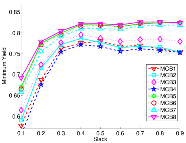
Figure 2: MCB Algorithms – Minimum Yield vs. Slack for small problem instances.

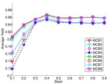
Figure 3: MCB Algorithms – Average Yield vs. Slack for small problem instances.

	% deg. from best
algorithm	avg.	max
MCB8	1.06	40.45
MCB5	1.60	38.67
MCB6	1.83	37.61
MCB7	3.91	40.71
MCB3	11.76	55.73
MCB2	14.21	48.30
MCB1	14.90	55.84
MCB4	17.32	46.95

Table 1: Average and Maximum percent degradation from best of the MCB algorithms for small problem instances.

We first present results only for our 8 multi-capacity bin packing algorithms to determine the best one. Figure 2 shows the achieved maximum minimum yield versus the memory slack averaged over small problem instances. As expected, as the memory slack increases all algorithms tend to do better although some algorithms seem to experience slight decreases in performance beyond a slack of $0.4$. Also expected, we see that the four algorithms that sort the tasks by descending order outperform the four that sort them by ascending order. Indeed, it is known that for bin packing starting with large items typically leads to better results on average.

The main message here is that MCB8 outperforms all other algorithms across the board. This is better seen in Table 1, which shows the average and maximum percent degradation from best for all algorithms. For a problem instance, the percent degradation from best of an algorithm is defined as the difference, in percentage, between the minimum yield achieved by an algorithm and the minimum yield achieved by the best algorithm for this instance. The average and maximum percent degradations from best are computed over all instances. We see that MCB8 has the lowest average percent degradation from best. MCB5, which corresponds to the algorithm in [28] performs well but not as well as MCB8. In terms of maximum percent degradation from best, we see that MCB8 ranks third, overtaken by MCB5 and MCB6. Examining the results in more details shows that, for these small problem instances, the maximum degradation from best are due to outliers. For instance, for the MCB8 algorithm, out of the 1,379 solved instances, there are only 155 instances for which the degradation from best if larger than 3%, and only 19 for which it is larger than 10%.

Figure 3 shows the average yield versus the slack (recall that the average yield is optimized in a second phase, as described in Section 3.5). We see here again that the MCB8 algorithm is among the very best algorithms.

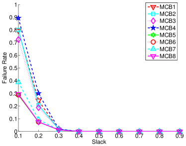
Figure 4: MCB Algorithms – Failure Rate vs. Slack for small problem instances.

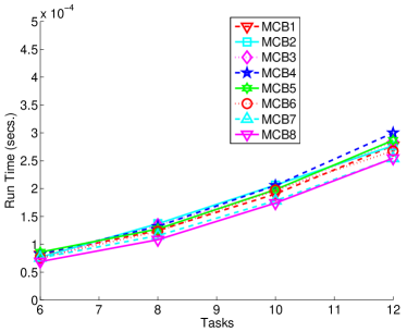
Figure 5: MCB Algorithms – Run time vs. Number of Tasks for small problems instances.

Figure 4 shows the failure rates of the 8 algorithms versus the memory slack. As expected failure rates decrease as the memory slack increases, and as before we see that the four algorithms that sort tasks by descending order outperform the algorithms that sort tasks by ascending order. Finally, Figure 5 shows the runtime of the algorithms versus the number of tasks. We use a 3.2GHz Intel Xeon processor. All algorithms have average run times under 0.18 milliseconds, with MCB8 the fastest by a tiny margin.

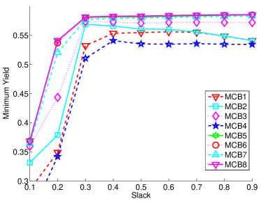
Figure 6: MCB Algorithms – Minimum Yield vs. Slack for large problem instances.

	% deg. from best
algorithm	avg.	max
MCB8	0.09	3.16
MCB5	0.25	3.50
MCB6	0.46	16.68
MCB7	1.04	48.39
MCB3	4.07	64.71
MCB2	8.68	46.68
MCB1	10.97	73.33
MCB4	14.80	61.20

Figure 7: Average and Maximum percent degradation from best of the MCB algorithms for large problem instances.

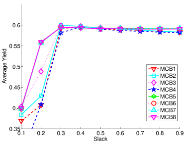
Figure 8: MCB Algorithms – Average Yield vs. Slack for large problem instances.

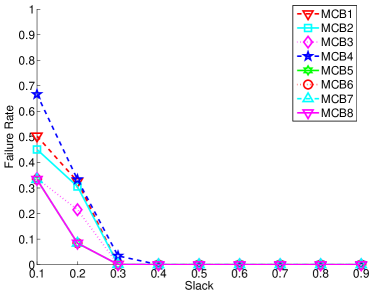
Figure 9: MCB Algorithms – Failure Rate vs. Slack for large problem instances.

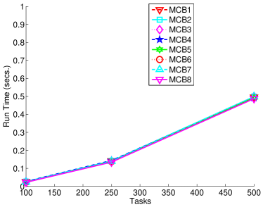
Figure 10: MCB Algorithms – Run time vs. Number of Tasks for large problem instances.

Figures 6,  8,  9, and 10 are similar to Figures 2,  3,  4, and 5, but show results for large problem instances. The message is the same here: MCB8 is the best algorithm, or closer on average to the best than the other algorithms. This is clearly seen in Table 7, which is similar to Table 1, and shows the average and maximum percent degradation from best for all algorithms for large problem instances. According to both metrics MCB8 is the best algorithm, with MCB5 performing well but not as well as MCB8.

In terms of run times, Figure 10 shows run times under one-half second for 500 tasks for all of the MCB algorithms. MCB8 is again the fastest by a tiny margin.

Based on our results we conclude that MCB8 is the best option among the 8 multi-capacity bin packing options. In all that follows, to avoid graph clutter, we exclude the 7 other algorithms from our overall results.

4.2.2 Small Problems

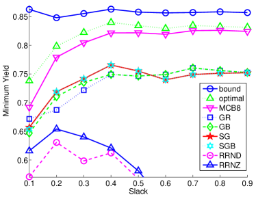
Figure 11: Minimum Yield vs. Slack for small problem instances.

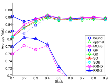
Figure 12: Average Yield vs. Slack for small problem instances.

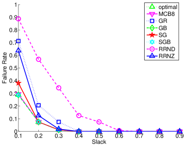
Figure 13: Failure Rate vs. Slack for small problem instances.

Figure 11 shows the achieved maximum minimum yield versus the memory slack in the system for our algorithms, the MILP solution, and for the solution of the rational LP, which is an upper bound on the achievable solution. The solution of the LP is only about 4% higher on average than that of the MILP, although it is significantly higher for very low slack values. The solution of the LP will be interesting for large problem instances, for which we cannot compute an exact solution. On average, the exact MILP solution is about 2% better than MCB8, and about 11% to 13% better than the greedy algorithms. All greedy algorithms exhibit roughly the same performance. The RRND and RRNZ algorithms lead to results markedly poorer than the other algorithms, with expectedly the RRNZ algorithm slightly outperforming the RRND algorithm. Interestingly, once the slack reaches 0.2 the results of both the RRND and RRNZ algorithms begin to worsen.

Figure 12 is similar to Figure 11 but plots the average yield. The solution to the rational LP, the MILP solution, the MCB8 solution, and the solutions produced by the greedy algorithms are all within a few percent of each other. As in Figure 11, when the slack is lower than 0.2 the relaxed solution is significantly better.

Figure 13 plots the failure rates of our algorithms. The RRND algorithm has the worst failure rate, followed by GR and then RRNZ. There were a total of 60 instances out of the 1,440 generated which were judged to be infeasible because the GLPK solver could not find a solution for them. We see that the MCB8, SG, and SGB algorithms have failure rates that are not significantly larger than that of the exact MILP solution. Out of the 1,380 feasible instances, the GB and SGB never fail to find a solution, the MCB8 algorithm fails once, and the SG algorithm fails 15 times.

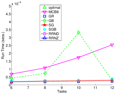
Figure 14: Run time vs. Number of Tasks for small problems instances.

Figure 14 shows the run times of the various algorithms on a 3.2GHz Intel Xeon processor. The computation time of the exact MILP solution is so much greater than that of the other algorithms that it cannot be seen on the graph. Computing the exact solution to the MILP took an average of 28.7 seconds, however there were 9 problem instances with solutions that took over 500 seconds to compute, and a single problem instance that required 11,549.29 seconds (a little over 3 hours) to solve. For the small problem instances the average run times of all greedy algorithms and of the MCB8 algorithm are under 0.15 milliseconds, with the simple GR and SG algorithms being the fastest. The RRND and RRNZ algorithms are significantly slower, with run times a little over 2 milliseconds on average; they also cannot be seen on the graph.

4.2.3 Large Problems

Figures 15, 16, 17, and 18 are similar to Figures 11, 12, 13, and 14 respectively, but for large problem instances. In Figure 15 we can see that MCB8 algorithm achieves far better results than any other heuristic. Furthermore, MCB8 is extremely close to the upper bound as soon as the slack is 0.3 or larger and is only 8% away from this upper bound when the slack is 0.2. When the slack is 0.1, MCB8 is 37% away from the upper bound but we have seen with the small problem instances that in this case the upper bound is significantly larger than the actual optimal (see Figure 11).

The performance of the greedy algorithms has worsened relative to the rational LP solution, on average 20% lower for slack values larger than 0.2. The GR and GB algorithms perform nearly identically, showing that backtracking does not help on the large problem instances. The RRNZ algorithm is again a poor performer, with a profile that, unexpectedly, drops as slack increases. The RRND algorithm not only achieved the lowest values for minimum yield, but also completely failed to solve any instances of the problem for slack values less than 0.4.

Figure 16 shows the achieved average yield values. The MCB8 algorithm again tracks the optimal for slack values larger than 0.3. A surprising observation at first glance is that the greedy algorithms manage to achieve higher average yields than the optimal or MCB algorithms. This is due to their lower achieved minimum yields. Indeed, with a lower minimum yield, average yield maximization is less constrained, making it possible to achieve higher average yield than when starting from and allocation optimal for the minimum yield. The greedy algorithms thus trade off fairness for higher average performance. The RRNZ algorithm starts out doing well for average slack, even better than GR or GB when the slack is low, but does much worse as slack increases.

Figure 17 shows that for large problem instances the GB and SGB algorithms have nearly as many failures as the GR and SG algorithms when slack is low. This suggests that the arbitrary bound of 500,000 placement attempts when backtracking, which was more than sufficient for the small problem set, has little affect on overall performance for the large problem set. It could thus be advisable to set the bound on the number of placement attempts based on the size of the problem set and time allowed for computation. The RRND algorithm is the only algorithm with a significant number of failures for slack values larger than 0.3. The SG, SGB and MCB8 algorithms exhibit the lowest failure rates, about 40% lower than that experienced by the other greedy and RRNZ algorithms, and more than 14 times lower than the failure rate of the RRND algorithm. Keep in mind that, based on our experience with the small problem set, some of the problem instances with small slacks may not be feasible at all.

Figure 18 plots the average time needed to compute the solution to VCSched on a 3.2GHz Intel Xeon for all the algorithms versus the number of jobs. The RRND and RRNZ algorithms require significant time, up to roughly 650 seconds on average for 500 tasks, and so cannot be seen at the given scale. This is attributed to solving the relaxed MILP using GLPK. Note that this time could be reduced significantly by using a faster solver (e.g., CPLEX [14]). The GB and SGB algorithms require significantly more time when the number of tasks is small. This is because the failure rate decreases as the number of tasks increases. For a given set of parameters, increasing the number of tasks decreases granularity. Since there is a relatively large number of unsolvable problems when the number of tasks is small, these algorithms spend a lot of time backtracking and searching though the solution space fruitlessly, ultimately stopping only when the bounded number of backtracking attempts is reached. The greedy algorithms are faster than the MCB8 algorithm, returning solutions in 15 to 20 milliseconds on average for 500 tasks as compared to nearly half a second for MCB8. Nevertheless, less than .5 seconds for 500 tasks is clearly acceptable in practice.

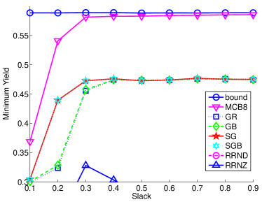
Figure 15: Minimum Yield vs. Slack for large problem instances.

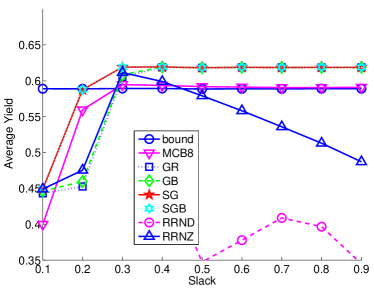
Figure 16: Average Yield vs. Slack for large problem instances.

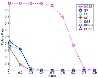
Figure 17: Failure Rate vs. Slack for large problem instances.

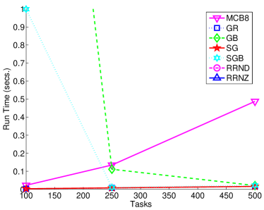
Figure 18: Run time vs. Number of Tasks for large problem instances.

4.2.4 Discussion

Our main result is that the multi-capacity bin packing algorithm that sorts tasks in descending order by their largest resource requirement (MCB8) is the algorithm of choice. It outperforms or equals all other algorithm nearly across the board in terms of minimum yield, average yield, and failure rate, while exhibiting relatively low run times. The sorted greedy algorithms (SG or SGB) lead to reasonable results and could be used for very large numbers of tasks, for which the run time of MCB8 may become too high. The use of backtracking in the algorithms GB and SGB led to performance improvements for small problem sets but not for large problem sets, suggesting that some sort of backtracking system with a problem-size- or run-time-dependent bound on the number of branches to explore could potentially be effective.

5 Parallel Jobs

5.1 Problem Formulation

In this section we explain how our approach and algorithms can be easily extended to handle parallel jobs that consist of multiple tasks (relaxing assumption H3). We have thus far only concerned ourselves with independent jobs that are both indivisible and small enough to run on a single machine. However, in many cases users may want to split up jobs into multiple tasks, either because they wish to use more CPU power in order to return results more quickly or because they wish to process an amount of data that does not fit comfortably within the memory of a single machine.

One naïve way to extend our approach to parallel jobs would be to simply consider the tasks of a job independently. In this case individual tasks of the same job could then receive different CPU allocations. However, in the vast majority of parallel jobs it is not useful to have some tasks run faster than others as either the job makes progress at the rate of the slowest task or the job is deemed complete only when all tasks have completed. Therefore, we opt to add constraints to our linear program to enforce that the CPU allocations of tasks within the same job must be identical. It would be straightforward to have more sophisticated constraints if specific knowledge about a particular job is available (e.g., task A should receive twice as much CPU as task B).

Another important issue here is the possibility of gaming the system when optimizing the average yield. When optimizing the minimum yield, a division of a job into multiple tasks that leads to a higher minimum yield benefits all jobs. However, when considering the average yield optimization, which is done in our approach as a second round of optimization, a problem arises because the average yield metric favors small tasks, that is, tasks that have low CPU requirements. Indeed, when given the choice to increase the CPU allocation of a small task or of a larger task, for the same additional fraction of CPU, the absolute yield increase would be larger for the small task, and thus would lead to a higher average yield. Therefore, an unscrupulous user might opt for breaking his/her job into unnecessarily many smaller tasks, perhaps hurting the parallel efficiency of the job, but acquiring an overall larger portion of the total available CPU resources, which could lead to shorter job execution time. To remedy this problem we use a per-job yield metric (i.e., total CPU allocation divided by total CPU requirements) during the average yield optimization phase.

The linear programming formulation with these additional considerations and constraints is very similar to that derived in Section 2.5. We again consider jobs $1..J$ and hosts $1..H$. But now each job $i$ consists of $T_{i}$ tasks. Since these jobs are constrained to be uniform, $\alpha_{i}$ represents the maximum CPU consumption and $m_{i}$ represents the maximum memory consumption of all tasks $k$ of job $i$. The integer variables $e_{ikj}$ are constrained to be either $0$ or $1$ and represent the absence or presence of task $k$ of job $i$ on host $j$. The variables $\alpha_{ikj}$ represent the amount of CPU allocated to task $k$ of job $i$ on host $j$.

$$\forall i,k,j \quad e_{ikj}\in\mathbb{N},$$ (12)

$$\forall i,k,j \quad\alpha_{ikj}\in\mathbb{Q},$$ (13)

$$\forall i,k,j 0\leq e_{ikj}\leq 1,$$ (14)

$$\forall i,k,j 0\leq\alpha_{ikj}\leq e_{ikj},$$ (15)

$$\forall i,k \sum_{j=1}^{H}e_{ikj}=1,$$ (16)

$$\forall j \sum_{i=1}^{J}\sum_{k=1}^{T_{i}}\alpha_{ikj}\leq 1,$$ (17)

$$\forall j \sum_{i=1}^{J}\sum_{k=1}^{T_{i}}e_{ikj}m_{i}\leq 1,$$ (18)

$$\forall i,k \sum_{j=1}^{H}\alpha_{ikj}\leq\alpha_{i},$$ (19)

$$\forall i,k,k^{\prime} \sum_{j=1}^{H}\alpha_{ikj}=\sum_{j=1}^{H}\alpha_{ik^{\prime}j},$$ (20)

$$\forall i \sum_{j=1}^{H}\sum_{k=1}^{T_{i}}\frac{\alpha_{ikj}}{T_{i}\times\alpha_{i}}\geq Y$$ (21)

Note that the final constraint is logically equivalent to the per-task yield since all tasks are constrained to have the same CPU allocation. The reason for writing it this way is to highlight that in the second phase of optimization one should maximize the average per-job yield rather than the average per-task yield.

5.2 Results

The algorithms described in Section 3 for the case of sequential jobs can be used directly for minimum yield maximization for parallel jobs. The only major difference is that the average per-task yield optimization phase needs to be changed for an average per-job optimization phase. As with the per-task optimization, we make the simplifying assumption that task placement decisions cannot be changed during this phase of the optimization. This simplification removes not only the difficulty of solving a MILP, but also allows us to avoid the enormous number of additional constraints which would be required to make sure that all of a given job’s tasks receive the same allocation while keeping the problem linear.

We present results only for large problem instances as defined in Section 4.1. We use the same experimental methodology as defined there as well. We only need a way to decide how many tasks comprise a parallel job. To this end, we use the parallel workload model proposed in [30], which models many characteristics of parallel workloads (derived based on statistical analysis of real-world batch system workloads). The model for the number of tasks in a parallel job uses a two-stage log-uniform distribution biased towards powers of two. We instantiate this model using the same parameters as in [30], assuming that jobs can consist of between 1 and 64 tasks.

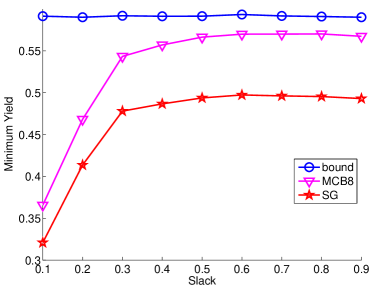
Figure 19: Minimum Yield vs. Slack for large problem instances for parallel jobs.

Figure 19 shows results for the SG and the MCB8 algorithms. We exclude all other greedy algorithms as they were all shown to be outperformed by SG, all other MCB algorithms because they were all shown to be outperformed by MCB8, as well as the RRND and RRNZ algorithms which were shown to perform poorly. The figure also shows the upper bound on optimal obtained assuming that $e_{ij}$ variables can take rational values. We see that MCB8 outperforms the SGB algorithm significantly and is close to the upper bound on optimal for slacks larger than $0.3$.

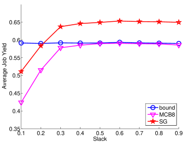
Figure 20: Average Yield vs. Slack for large problem instances for parallel jobs.

Figure 20 shows the average job yield. We see the same phenomenon as in Figure 16, namely that the greedy algorithm can achieve higher average yield because it starts from a lower minimum yield, and thus has more options to push the average yield higher (thereby improving average performance at the expense of fairness).

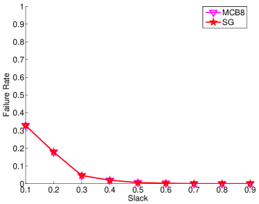
Figure 21: Failure Rate vs. Slack for large problem instances for parallel jobs.

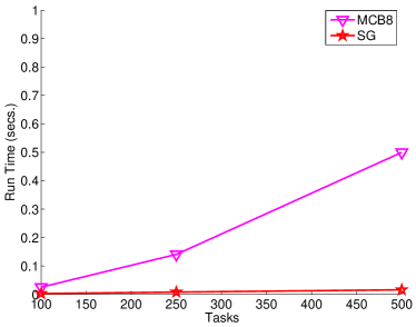
Figure 22: Runtime vs. Number of Tasks for large problem instances for parallel jobs.

Figure 21 shows the failure rates of the MCB8 and SG algorithms, which are identical. Finally Figure 22 shows the run time of both algorithms. We see that the SG algorithm is much faster than the MCB8 algorithm (by roughly a factor 32 for 500 tasks). Nevertheless, MCB8 can still compute an allocation in under one half a second for 500 tasks.

Our conclusions are similar to the ones we made when examining results for sequential jobs: in the case of parallel jobs the BCB8 algorithm is the algorithm of choice for optimizing minimum yield, while the SGB algorithm could be an alternate choice if the number of tasks is very large.

6 Dynamic Workloads

In this section we study resource allocation in the case when assumption H4 no longer holds, meaning that the workload is no longer static. We assume that job resource requirements can change and that jobs can join and leave the system. When the workload changes, one may wish to adapt the schedule to reach a new (nearly) optimal allocation of resources to the jobs. This adaptation can entail two types of actions: (i) modifying the CPU fractions allocated to some jobs; and (ii) migrating jobs to different physical hosts. In what follows we extend the linear program formulation derived in Section 2.5 to account for resource allocation adaptation. We then discuss how current technology can be used to implement adaptation with virtual clusters.

6.1 Mixed-Integer Linear Program Formulation

One difficult question for resource allocation adaptation, regardless of the context, is whether the adaptation is “worth it.” Indeed, adaptation often comes with an overhead, and this overhead may lead to a loss of performance. In the case of virtual cluster scheduling, the overhead is due to VM migrations. The question of whether adaptation is worthwhile is often based on a time horizon (e.g., adaptation is not worthwhile if the workload is expected to change significantly in the next 5 minutes) [45, 41]. In virtual cluster scheduling, as defined in this paper, jobs do not have time horizons. Therefore, in principle, the scheduler cannot reason about when resource needs will change. It may be possible for the scheduler to keep track of past workload behavior to forecast future workload behavior. Statistical workload models have been built (see [30, 29] for models and literature reviews). Techniques to make predictions based on historical information have been developed (see [1] for task execution time models and a good literature review). Making sound short-term decisions for resource allocation adaptation requires highly accurate predictions, so as to carry out precise cost-benefit analyses of various adaptation paths. Unfortunately, accurate point predictions (rather than statistical characterizations) are elusive due to the inherently statistical and transient nature of the workload, as seen in the aforementioned works. Furthermore, most results in this area are obtained for batch scheduling environments with parallel scientific applications, and it is not clear whether the obtained models would be applicable in more general settings (e.g., cloud computing environments hosting internet services).

Faced with the above challenge, rather than attempting arduous statistical forecasting of adaption cost and pay-off, we side-step the issue and propose a pragmatic approach. We consider schedule adaptation that attempts to achieve the best possible yield, but so that job migrations do not entail moving more than some fixed number of bytes, $B$ (e.g., to limit the amount of network load due to schedule adaptation). If $B$ is set to $0$, then the adaptation will do the best it can without using migration whatsoever. If $B$ is above the sum of the job sizes (in bytes of memory requirement), then all jobs could be migrated.

It turns out that this adaptation scheme can be easily formulated as a mixed-integer linear program. More generally, the value of $B$ can be chosen so that it achieves a reasonable trade-off between overhead and workload dynamicity. Choosing the best value for $B$ for a particular system could however be difficult and may need to be adaptive as most workloads are non-stationary. A good approach is likely to pick relatively smaller values of $B$ for more dynamic workload. We leave a study of how to best tune parameter $B$ for future work.

We use the same notations and definitions as in Section 2.5. In addition, we consider that some jobs are already assigned to a host: $\bar{e}_{ij}$ is equal to $1$ if job $i$ is already running on host $j$, and $0$ otherwise. For reasons that will be clear after we explain our constraints, we simply set $\bar{e}_{ij}$ to $1$ for all $j$ if job $i$ corresponds to a newly arrived job. Newly departed jobs need not be taken into account. We can now write a new set of constraints as follows:

$$\forall i,j \quad e_{ij}\in\mathbb{N},$$ (22)

$$\forall i,j \quad\alpha_{ij}\in\mathbb{Q},$$ (23)

$$\forall i,j 0\leq e_{ij}\leq 1,$$ (24)

$$\forall i,j 0\leq\alpha_{ij}\leq e_{ij},$$ (25)

$$\forall i \sum_{j=1}^{H}e_{ij}=1,$$ (26)

$$\forall j \sum_{i=1}^{T}\alpha_{ij}\leq 1,$$ (27)

$$\forall j \sum_{i=1}^{T}e_{ij}m_{i}\leq 1\;$$ (28)

$$\forall i \sum_{j=1}^{H}\alpha_{ij}\leq\alpha_{i}\;$$ (29)

$$\forall i \sum_{j=1}^{H}\frac{\alpha_{ij}}{\alpha_{i}}\geq Y$$ (30)

$$\sum_{i=1}^{T}\sum_{j=1}^{H}(1-\bar{e}_{ij})e_{ij}m_{i}\leq B$$ (31)

The objective, as in Section 2.5, is to maximize $Y$. The only new constraint is the last one. This constraint simply states that if job $i$ is assigned to a host that is different from the host to which it was assigned previously, then it needs to be migrated. Therefore, $m_{i}$ bytes need to be transferred. These bytes are summed over all jobs in the system to ensure that the total number of bytes communicated for migration purposes does not exceed $B$. Note that this is still a linear program as $\bar{e}_{ij}$ is not a variable but a constant. Since for newly arrived jobs we set all $\bar{e}_{ij}$ values to $1$, we can see that they do not contribute to the migration cost. Note that removing $m_{i}$ in the last constraint would simply mean that $B$ is a bound on the total number of job migrations allowed during schedule adaptation.

We leave the development of heuristic algorithms for solving the above linear program for future work.

6.2 Technology Issues for Resource Allocation Adaptation

In the linear program in the previous section nowhere do we account for the time it takes to migrate a job. While a job is being migrated it is presumably non-responsive, which impacts the yield. However, modern VM monitors support “live migration” of VM instances, which allows migrations with only milliseconds of unresponsiveness [13]. There could be a performance degradation due to memory pages being migrated between two physical hosts. Resource allocation adaptation also requires quick modification of the CPU share allocated to a VM instance (assumption H5). We validate this assumption in Section 7 and find that, indeed, CPU shares can be modified accurately in under a second.

7 Evaluation of the Xen Hypervisor

Assumption H5 in Section 2.2 states that VM technology allows for precise, low-overhead, and quickly adaptable sharing of the computational capabilities of a host across CPU-bound VM instances. Although this seems like a natural expectation, we nevertheless validate this assumption with state-of-the-art virtualization technology, namely, the Xen VM monitor [8]. While virtualization can happen inside the operating system (e.g, Virtual PC [34], VMWare [53]), Xen runs between the hardware and the operating system. It thus requires either a modified operating system (“paravirtualization”) or hardware support for virtualization (“hardware virtualization” [21]). In this work we use Xen 3.1 on a dual-CPU 64-bit machine with paravirtualization. All our VM instances use identical 64-bit Fedora images, are allocated 700MB of RAM, and run on the same physical CPU. The other CPU is used to run the experiment controller. All our VM instances perform continuous CPU-bound computations, that is, $100\times 100$ double precision matrix multiplications using the LAPACK DGEMM routine [5].

Our experiments consist in running from one to ten VM instances with specified “cap values”, which Xen uses to control what fraction of the CPU is allocated to each VM. We measure the effective compute rate of each VM instance (in number of matrix multiplications per seconds). We compare this rate to the expected rate, that is, the cap value times the compute rate measured on the raw hardware. We can thus ascertain both the accuracy and the overhead of the CPU-sharing in Xen. We also conduct experiments in which we change cap values on-the-fly and measure the delay before the effective compute rates are in agreement with the new cap values.

Due to space limitations we only provide highlights of our results and refer the reader to a technical report for full details [43]. We found that Xen imposes a minimal overhead (on average a 0.27% slowdown). We also found that the absolute error between the effective compute rate and the expected compute rate was at most 5.99% and on average 0.72%. In terms of responsiveness, we found that the effective compute rate of a VM becomes congruent with a cap value less than one second after that cap value was changed. We conclude that, in the case of CPU-bound VM instances, CPU-sharing in Xen is sufficiently accurate and responsive to enable fractional and dynamic resource allocations as defined in this paper.

8 Related Work

The use of virtual machine technology to improve parallel job reliability, cluster utilization, and power efficiency is a hot topic for research and development, with groups at several universities and in industry actively developing resource management systems [32, 3, 2, 19, 42]. This paper builds on top of such research, using the resource manager intelligently to optimize a user-centric metric that attempts to capture common ideas about fairness among the users of high-performance systems.

Our work bears some similarities with gang scheduling. However, traditional gang scheduling approaches suffer from problems due to memory pressure and the communication expense of coordinating context switches across multiple hosts [38, 9]. By explicitly considering task memory requirements when making scheduling decisions and using virtual machine technology to multiplex the CPU resources of individual hosts our approach avoids these problems.

Above all, our approach is novel in that we define and optimize for a user-centric metric which captures both fairness and performance in the face of unknown time horizons and fluctuating resource needs. Our approach has the additional advantage of allowing for interactive job processes.

9 Limitations and Future Directions

In this work we have made two key assumptions. The first assumption is that VM instances are CPU-bound (assumption H1), which made it possible to validate assumption H5 in Section 7. However, in reality, VM instances may have composite needs that span multiple resources, including the network, the disk, and the memory bus. The second assumption is that resource needs are known (assumption H2). However, this typically does not hold true in practice as users do not know precise resource needs of their applications. When assumption H1 does not hold, the challenge is to model composite resource needs in the definition of the resource allocation problem, and to share these various resources among VM instances in practice.

In practice, CPU and network resources are strongly dependent within a virtual machine monitor environment. To ensure secure isolation, VM monitors interpose on network communication, adding CPU overhead as a result. Experience has shown that, because of this dependence, one can capture network needs in terms of additional CPU need [20]. Therefore, it should be straightforward to modify our approach to account for network resource usage. In terms of disk usage, we note that virtual cluster environments typically use network-attached storage to simplify VM migration. As a result, disk usage is subsumed in network usage. In both cases one should then be able to both model and precisely share network and disk usage. Much more challenging is the modeling and sharing of the memory bus usage, due to complex and deep memory hierarchies on multi-core processors. However, current work on Virtual Private Machines points to effective ways for achieving sharing and performance isolation among VM instances of microarchitecture resources [37], including the memory hierarchy [36].

In terms of discovering VM instance resource needs, a first approach is to use standard services for tracking VM resource usage across a cluster and collecting the information as input into a cluster system scheduler (e.g., the XenMon VM monitoring facility in Xen [15]. Application resource needs inside a VM instance can be discovered via a combination of introspection and configuration variation. With introspection, for example, one can deduce application CPU needs by inferring process activity inside of VMs [47], and memory pressure by inferring memory page eviction activity [48]. This kind of monitoring and inference provides one set of data points for a given system configuration. By varying the configuration of the system, one can then vary the amount of resources given to applications in VMs, track how they respond to the addition or removal of resources, and infer resource needs. Experience with such techniques in isolation has shown that they can be surprisingly accurate [47, 48]. Furthermore, modeling resource needs across a range of configurations with high accuracy is less important than discovering where in that range the application experiences an inflection point (e.g., cannot make use of further CPU or memory) [17, 40].

10 Conclusion

In this paper we have proposed a novel approach for allocating resources among competing jobs, relying on Virtual Machine technology and on the optimization of a well-defined metric that captures notions of performance and of fairness. We have given a formal definition of a base problem, have proposed several algorithms to solve it, and have evaluated these algorithms in simulation. We have identified a promising algorithm that runs quickly, is on par with or better than its competitors, and is close to optimal in terms of our objective function. We have then discussed several extensions to our approach to solve more general problems, namely when jobs are parallel, when the workload is dynamic, when job resource needs are composite, and when job resource needs are unknown.

Future directions include the development of algorithms to solve the resource allocation adaptation problem, and of strategies for estimating job resource needs accurately. Our ultimate goal is to develop a new resource allocator as part of the Usher system [32], so that our algorithms and techniques can be used as part of a practical system and evaluated in practical settings.

References

- [1] Backfilling Using System-Generated Predictions Rather than User Runtime Estimates. IEEE Transactions on Parallel and Distributed Systems, 18(6):789–803, 2007.
- [2] Citric xenserver enterprise edition. http://www.xensource.com/products/Pages/XenEnterprise.aspx, 2008.
- [3] Virtualcenter. http://www.vmware.com/products/vi/vc, 2008.
- [4] Amazon Elastic Compute Cloud. http://aws.amazon.com/ec2.
- [5] E. Anderson, Z. Bai, C. Bischof, S. Blackford, J. Demmel, J. Dongarra, J. Du Croz, A. Greenbaum, S. Hammarling, A. McKenney, and D. Sorensen. LAPACK Users’ Guide Third Edition. Society for Industrial and Applied Mathematics, 1999.
- [6] K. Baker. Introduction to Sequencing and Scheduling. Wiley, 1974.
- [7] N. Bansal and M. Harchol-Balter. Analysis of SRPT Scheduling: Investigating Unfairness. In Proceedings of ACM SIGMETRICS 2001 Conference on Measurement and Modeling of Computer Systems, pages 279–290, June 2001.
- [8] P. Barham, B. Dragovic, K. Fraser, S. Hand, T. Harris, A. Ho, R. Neugebauer, I. Pratt, and A. Warfield. Xen and the Art of Virtualization. In Proceedings of the ACM Symposium on Operating Systems Principles, pages 164–177, October 2003.
- [9] A. Batat and D. Feitelson. Gang scheduling with memory considerations. In Proceedings of the 14th International Parallel and Distributed Processing Symposium, pages 109–114, 2000.
- [10] M. Bender, S. Chakrabarti, and S. Muthukrishnan. Flow and Stretch Metrics for Scheduling Continuous Job Streams. In Proceedings of the 9th Annual ACM-SIAM Symposium On Discrete Algorithms (SODA’98), pages 270–279, 1998.
- [11] M. Bender, S. Muthukrishnan, and R. Rajamaran. Approximation Algorithms for Average Stretch Scheduling. Journal of Scheduling, 7(3):195–222, 2004.
- [12] J. Buisson, F. André, and J.-L. Pazat. A Framework for Dynamic Adaptation of Parallel Components. In Proceedings of the International Conference ParCo, pages 65–72, 2005.
- [13] Christopher Clark and Keir Fraser and Steven Hand and Jacob Gorm Hansen and Eric Jul and Christian Limpach and Ian Pratt and Andrew Warfield. Live Migration of Virtual Machines. In Proceedings of the 2nd Conference on Symposium on Networked Systems Design and Implementation (NSDI’05), pages 273–286, April 2005.
- [14] CPLEX. http://www.ilog.com/products/cplex/.
- [15] Diwaker Gupta and Rob Gardner and Ludmila Cherkasova. XenMon: QoS Monitoring and Performance Profiling Tool. Technical Report HPL-2005-187, Hewlett-Packard Labs, 2005.
- [16] D. G. Feitelson. Metrics for parallel job scheduling and their convergence. In Proceedings of Job Scheduling Strategies for Parallel Processing (JSPP), pages 188–206, 2001.
- [17] Y. Fu, J. S. Chase, B. Chun, S. Schwab, and A. Vahdat. SHARP: An Architecture for Secure Resource Peering. In Proceedings of the 19th ACM Symposium on Operating System Principles (SOSP), October 2003.
- [18] M. R. Garey and D. S. Johnson. Computers and Intractability, a Guide to the Theory of NP-Completeness. W.H. Freeman and Company, 1979.
- [19] L. Grit, D. Itwin, V. Marupadi, P. Shivam, A. Yumerefendi, J. Chase, and J. Albrecth. Harnessing Virtual Machine Resource Control for Job Management. In Proceedings of HPCVirt 2007, November 2007.
- [20] D. Gupta, L. Cherkasova, and A. Vahdat. Comparison of the Three CPU Schedulers in Xen. ACM SIGMETRICS Performance Evaluation Review (PER), 35(2):42–51, September 2007.
- [21] Intel Virtualization Technology (Intel VT). http://www.intel.com/technology/virtualization/index.htm.
- [22] IBM Introduces Ready-to-Use Cloud Computing. http://www-03.ibm.com/press/us/en/pressrelease/22613.wss, 2007.
- [23] Jeff Dean and Sanjay Ghemawat. MapReduce: Simplified data processing on large clusters. In Proceedings of the 6th OSDI, pages 137–150, December 2004.
- [24] Jonathan G. Koomey. Estimating Total Power Consumption by Servers in the U.S. and the World. http://enterprise.amd.com/Downloads/svrpwrusecompletefinal.pdf, February 2007.
- [25] L. Kalé, S. Kumar, and J. DeSouza. A Malleable-Job System for Time-Shared Parallel Machines. In Proceedings of the 2nd IEEE/ACM International Symposium on Cluster Computing and the Grid (CCGRID), page 230, 2002.
- [26] C. B. Lee and A. Snavely. Precise and Realistic Utility Functions for User-Centric Performance Analysis of Schedulers. In Proceedings of IEEE Symposium on High-Performance Distributed Computing (HPDC-16), June 2007.
- [27] A. Legrand, A. Su, and F. Vivien. Minimizing the Stretch when Scheduling Flows of Divisible Requests. Journal of Scheduling, 2008. to appear, DOI: 10.1007/s10951-008-0078-4.
- [28] W. Leinberger, G. Karypis, and V. Kumar. Multi-capacity bin packing algorithms with applications to job scheduling under multiple constraints. In Proceedings of the International Conference on Parallel Processing, pages 404–412, 1999.
- [29] H. Li. Workload Dynamics on Clusters and Grids. Journal of Supercomputing, 2008. on-line publication.
- [30] U. Lublin and D. Feitelson. The Workload on Parallel Supercomputers: Modeling the Characteristics of Rigid Jobs. Journal of Parallel and Distributed Computing, 63(11), 2003.
- [31] L. Marchal, Y. Yang, H. Casanova, and Y. Robert. Steady-state scheduling of multiple divisible load applications on wide-area distributed computing platforms. 20(3):365–381, 2006.
- [32] M. McNett, D. Gupta, A. Vahdat, and G. M. Voelker. Usher: An extensible framework for managing clusters of virtual machines. In Proceedings of Lisa 2007, 2007.
- [33] Michael Isard and Mihai Budiu and Yuan Yu and Andrew Birrell and Dennis Fetterly. Dryad: Distributed Data-Parallel Programs from Sequential Building Blocks. In Proceedings of the European Conference on Computer Systems (EuroSys), March 2007.
- [34] Microsoft Virtual PC. http://www.microsoft.com/windows/products/winfamily/virtualpc/default.m%spx.
- [35] S. Muthukrishnan, R. Rajaraman, A. Shaheen, and J. Gehrke. Online Scheduling to Minimize Average Stretch. In Proceedings of the IEEE Symposium on Foundations of Computer Science, pages 433–442, 1999.
- [36] K. Nesbit, J. Laudon, and J. Smith. Virtual Private Caches. In Proceedings of the 34th Annual International Symposium on Computer Architecture (ISCA), June 2007.
- [37] K. Nesbit, M. Moreto, F. Cazorla, A. Ramirez, and M. Valero. Multicore Resource Management. IEEE Micro, May-June 2008.
- [38] J. Ousterhout. Scheduling Techniques for Concurrent Systems. In Proceedings of the 3rd International Conferance on Distributed Computing Systems, pages 22–30, 1982.
- [39] A. H. Project. Hadoop. http://hadoop.apache.org/.
- [40] R. H. Patterson and G. A. Gibson and E. Ginting and D. Stodolsky and J. Zelenka. Informed Prefetching and Caching. In Proceedings of the 15th Symposium of Operating Systems Principles, October 1995.
- [41] R. L. Ribler, H. Simitci, and D. A. Reed. The Autopilot Performance-Directed Adaptive Control System. Future Generation Computer Systems, 18(1), 2001.
- [42] P. Ruth, R. Junghwan, D. Xu, R. Kennell, and S. Goasguen. Autonomic Live Adaptation of Virtual Computational Environments in a Multi-Domain Infrastructure. In Proceedings of the IEEE International Conference on Autonomic Computing, June 2006.
- [43] D. Schanzenbach and H. Casanova. Accuracy and Responsiveness of CPU Sharing Using Xen’s Cap Values. Technical Report ICS2008-05-01, Computer and Information Sciences Dept., University of Hawai‘i at Mānoa, May 2008. available at http://www.ics.hawaii.edu/research/tech-reports/ICS2008-05-01.pdf/view.
- [44] U. Schwiegelshohn and R. Yahyapour. Fairness in parallel job scheduling. Journal of Scheduling, 3(5):297–320, 2000.
- [45] O. Sievert and H. Casanova. A Simple MPI Process Swapping Architecture for Iterative Applications. International Journal of High Performance Computing Applications, 18(3):341–352, 2004.
- [46] A. Sodan and X. Huang. Adaptive Time/Space Sharing with SCOJO. International Journal of High Performance Computing and Networking, 4(5/6):256–269, 2006.
- [47] Stephen T. Jones and Andrea C. Arpaci-Dusseau and Remzi H. Arpaci-Dusseau. Antfarm: Tracking Processes in a Virtual Machine Environment. In Proceedings of the USENIX Annual Technical Conference (USENIX ’06), June 2006.
- [48] Stephen T. Jones and Andrea C. Arpaci-Dusseau and Remzi H. Arpaci-Dusseau. Geiger: Monitoring the Buffer Cache in a Virtual Machine Environment. In Proceedings of Architectural Support for Programming Languages and Operating Systems (ASPLOS XII), October 2006.
- [49] Top500 supercomputer sites. http://www.top500.org, 2008.
- [50] U.S. Environmental Protection Agency. Report to Congress on Server and Data Center Energy Efficiency. http://www.energystar.gov/ia/partners/prod_development/downloads/EPA_Da%tacenter_Report_Congress_Final1.pdf, August 2007.
- [51] G. Utrera, J. Corbalá, and J. Labarta. Implementing Malleability on MPI Jobs. In Proceedings of 13th International Conference on Parallel Archtecture and Compilation Techniques (PACT), pages 215–224, 2004.
- [52] S. Vadhiyar and J. Dongarra. SRS: A Framework for Developing Malleable and Migratable Parallel Applications for Distributed Systems. Parallel Processing Letters, 13(2):291–312, 2003.
- [53] VMware. http://www.vmware.com/.