Stochastic resonance with matched filtering

Abstract

Along with the development of interferometric gravitational wave detector, we enter into an epoch of gravitational wave astronomy, which will open a brand new window for astrophysics to observe our universe. Almost all of the data analysis methods in gravitational wave detection are based on matched filtering. Gravitational wave detection is a typical example of weak signal detection, and this weak signal is buried in strong instrument noise. So it seems attractable if we can take advantage of stochastic resonance. But unfortunately, almost all of the stochastic resonance theory is based on Fourier transformation and has no relation to matched filtering. In this paper we try to relate stochastic resonance to matched filtering. Our results show that stochastic resonance can indeed be combined with matched filtering for both periodic and non-periodic input signal. This encouraging result will be the first step to apply stochastic resonance to matched filtering in gravitational wave detection. In addition, based on matched filtering, we firstly proposed a novel measurement method for stochastic resonance which is valid for both periodic and non-periodic driven signal.

I introduction

Since the concept of stochastic resonance (SR) was originally put forward in the seminal papers by Benzi and others benzi , it has continuously attracted considerable attention review . SR was subsequently found to occur in many kinds of nonlinear systems bezrukov , even linear systems with multiplicative noise berdichevsky and diverse fields. Not only classical system but also quantum system quantum show SR behavior. Generally, SR emerged as a paradigm whose universal character was shown to be intimately related to the pervasiveness dykman of the fluctuation-dissipation theorem landau . The possible use of SR in connection with weak signal detection experiments jung91 ; gong92 ; inchiosa ; loerincz96 ; galdi98a ; galdi98b , with special reference to gravitational wave detection, was suggested since the infancy of SR gammaitoni89 . The application of stochastic resonance to gravitational wave detection includes two aspects, one is data analysis galdi98a , and the other is related to detector itself karapetyan04 . As to data analysis method, the research about stochastic resonance almost all use Fourier transformation method to deal with the data with noise. On the other hand, the data analysis method in gravitational wave detection community is mainly the so called matched filtering method, i.e. maximizing the likelihood ratio over the parameters of expected signal templates thorne87 ; cutler94 ; owen99 ; babak . So it is interesting to investigate whether we can combine the advanced data analysis method used in gravitational wave detection, matched filtering, with stochastic resonance. In this work, we will study whether the stochastic resonance phenomena can be observed also with matched filtering method to do data analysis. Our work shows that stochastic resonance does emerge with matched filtering data analysis method for periodic signal, corresponding to the periodic gravitational waves; chirp signal, corresponding to the gravitational wave radiated from merging black holes or neutron stars and even random pulse signals.

Till now we have three kinds of methods to characterize stochastic resonance. The first one is power spectrum include output signal power itself and the ratio of output signal power to noise background. This kind of measurement method is most convenient and popular when dealing with stochastic resonance. But the disadvantage of this method is that it can only deal with periodic stochastic resonance. The second method is residence time distribution lofstedt94 . The third one is information theoretic measures which includes the Shannon transinformation rate heneghan96 ; the Fisher information greenwood00 ; Kullback, Shannon and other kinds of entropies entropy ; and information-theoretic distance measures robinson98 ; collins95 . In this aspect, our work shows that matched filtering method can be looked as a novel measurement method to characterize stochastic resonance. The method of matched filtering is very robust that it can characterize both periodic and non-periodic stochastic resonance.

This paper is organized as following. In section II, we will give a brief review of matched filtering method used in gravitational wave data analysis. Then we present out our model equations used in this paper in section III. In section IV, we give out our result on stochastic resonance with matched filtering method. At last we discuss our result and its implications in section V.

II brief review of matched filtering techniques used in gravitational wave detection

First we flesh out the brief description of matched filtering techniques used in gravitational wave detection thorne87 . Assume our data stream takes form like

$$h(t)=s(t)+n(t),$$ (1)

where $s(t)$ is signal, while $n(t)$ is Gaussian white noise. The likelihood ratio is defined as cutler94 ; owen99

$${\cal M}\equiv\max_{t_{c}}\frac{\langle h,u(t-t_{c})\rangle}{\text{rms}\langle u,u\rangle}.$$ (2)

Here $u$ is the template determined by parameter in some space used to filter the data stream $h(t)$. The maximal value is taken with respect to the time delay $t_{c}$ of the template. When the signal is periodic or almost periodic the maximal value can be equivalently taken respect to the initial phase of template. And the inner product is given by

$$\langle a,b\rangle \equiv 4\text{Re}\left[\int_{0}^{\infty}\frac{\tilde{a}^{*}(f)\tilde{b}(f)}{S_{n}(f)}df\right]$$ (3)

$$= 2\int^{\infty}_{0}\frac{\tilde{a}^{*}(f)\tilde{b}(f)+\tilde{a}(f)\tilde{b}^{*}(f)}{S_{n}(f)}df.$$

It is the noise-weighted cross-correlation between $a$ and $b$. Here $\tilde{a}(f)$ stands for the Fourier transform of $a(t)$

$$\tilde{a}(f)\equiv\int_{-\infty}^{\infty}e^{i2\pi ft}a(t)dt,$$ (4)

and $*$ stands for complex conjugate. $S_{n}(f)$ is the one-sided power spectral noise density of the noise stream $n(t)$

$$S_{n}(f)\equiv 2\text{E}[|\tilde{n}(f)|^{2}],$$ (5)

where E[ ] denotes the expectation value over an ensemble of realizations of the noise. Since our data are all real, we can use one-sided power spectral instead of two-sided one. Above description is in frequency domain. In time domain, the inner product (3) takes form cutler94

$$\langle a,b\rangle\equiv\int_{-\infty}^{\infty}\int_{-\infty}^{\infty}a(t)w(t-\tau)b(\tau)dtd\tau,$$ (6)

where $w(t)$ is Wiener’s optimal filter kantz97 , which can be approximated as

$$w(t)\approx\int_{-\infty}^{\infty}e^{-i2\pi ft}\frac{1}{S_{n}(f)}df.$$ (7)

Then the task of data analysis in gravitational wave detection is to maximize the likelihood ratio ${\cal M}$ over the parameters space of expected signal templates and then fix a detection threshold on this statistics. The detection threshold is simply established by the desired level of false alarm probability. The maximum likelihood is compared with the aforementioned threshold and a detection is announced whenever the threshold is crossed.

In most pragmatic cases, the assumption of Gaussianness and whiteness to the noise is not valid, especially when noise passes through a nonlinear system, such as the system considered in this work. So the Wiener’s filter (7) is not valid any more. Therefore, we adopt the matched filtering method and the idea of Horner efficiency in optics caulfield82 to define matched ratio as

$${\cal M}=\max_{t_{c}\in\Delta}\frac{\int_{-\infty}^{\infty}|\int_{-\infty}^{\infty}h(t-\tau)u(\tau-t_{c})d\tau|dt}{\int_{-\infty}^{\infty}|h(t)|dt\int_{-\infty}^{\infty}|u(t)|dt},$$ (8)

where $h(t)$ is the data stream and $u(t)$ is the template as above. $t_{c}$ is the time delay for the template. $\Delta$ is the time delay range where the delay time is taken from. Theoretically $\Delta=(-\infty,+\infty)$, but it is impossible to take this infinity range practically. In practice, if the system has some characteristic time scale (such as the period of periodic system), this $\Delta$ can be taken as this time scale directly. Otherwise, there is an ambiguity to set this range. In the following sections we will come back to this problem and propose one trick to solve it. Different to equation (1), now $n(t)$ may be any kind of noise, white or colorful, Gaussian or non-Gaussian. So our quantity (8) will be valid in more general case than equation (2). Here the template is the signal profile we expected, and the different expected signal profiles up to a scale are looked as one template because we have already taken normalization in equation (8). Since we do not know when the expected signal will begin in the data stream, we need take the maximal value respect to the delay time $t_{c}$.

III model equation

The model equation used in this paper is the famous overdamped bistable system hu91

$$\dot{X}=aX-bX^{3}+S_{p}(t)+\Gamma(t),$$ (9)

with

$$\langle\Gamma(t)\rangle=0,\langle\Gamma(t)\Gamma(t^{\prime})\rangle=2D\delta(t-t^{\prime}).$$ (10)

$a$ and $b$ are two parameters. We set $a=b=1$ in this paper. This system has been widely investigated in stochastic resonance literature hu91 ; bistable ; hu92 . But all the studies used Fourier transformation method to do the data analysis. While in this paper we will adopt popular method used in gravitational wave detection—matched filtering method instead. $S_{p}(t)$ is the signal which is the input signal of our system. If we take our model equation as the toy model equation of gravitational wave detector, $S_{p}(t)$ is nothing but the gravitational wave signal. If we take our model equation as the afterward analysis tools for gravitational wave data analysis, $S_{p}(t)$ is the raw data stream of the gravitational wave detector’s output, which includes signal itself and noise. In the following we take the former viewpoint. As to numerical method, the stochastic Runge-Kutta algorithm risken is used in this work to simulate equation (9). The time step is set as $\Delta t=0.1$.

We take $200$ systems to realize the random process and take the ensemble average to analyze the random data stream produced by numerical method. Then our measurement quantity of stochastic resonance becomes the ensemble average of equation (8), i.e. $E[{\cal M}]$. More explicitly, the measurement quantity we introduced in this work to characterize stochastic resonance is

$$E[{\cal M}]=\frac{1}{N}\sum_{i=1}^{N}\max_{t_{c}\in\Delta}\frac{\int_{-\infty}^{\infty}|\int_{-\infty}^{\infty}h_{i}(t-\tau)u(\tau-t_{c})d\tau|dt}{\int_{-\infty}^{\infty}|h_{i}(t)|dt\int_{-\infty}^{\infty}|u(t)|dt}.$$ (11)

Here $h_{i}(t)$ is the data stream from i’th system. $N$ is the number of the systems in the ensemble. In practice, $h$ and $u$ are two arrays of numbers. Let us assume the length of the array is $m$. Then the convolution $\int_{-\infty}^{\infty}h_{i}(t-\tau)u(\tau-t_{c})d\tau$ can be done with standard algorithm. And we adopted rectangular method to approximate the other integral. We need pay more attention to the time delay problem since our data array is finite. In practice, we take the elements from number $\frac{t_{c}}{\Delta t}$ to $m$ of original discretized data stream $u$ for delayed template, while the data stream $h$ is correspondingly taken as the elements from number $1$ to $m-\frac{t_{c}}{\Delta t}+1$ of original array. Here $\Delta t$ is the sample time between the nearest two elements of the array which is the time step of the numerical simulation in our work.

IV stochastic resonance with matched filtering method

In this section we present our main result on stochastic resonance with matched filtering method. We find that stochastic resonance shows up perfectly with characteristic quantity (11) no mater what kind of input signal we use. Our input signal includes periodic one, which corresponds to the periodic gravitational waves; chirp signal, corresponding to the gravitational wave radiated from merging black holes or neutron stars and random pulse ones. All of these stochastic resonance phenomena can be described well by the quantity (11) we first introduced in this paper.

IV.1 periodic input

Firstly, we set the input signal in equation (9) as sinusoidal function of time

$$S_{p}(t)=A\cos(\omega t),$$ (12)

with $\omega=0.2,A=0.05$ closely following hu91 . This signal can model periodic gravitational wave very well. Periodic gravitational waves are emitted by various astrophysical sources. They carry important information on their sources (e.g., spinning neutron stars, accreting neutron stars) and also on fundamental physics, since their nature can test the model of general relativity. As to the expected profile of output signal we take $S_{p}(t)$ directly as our template. In numerical simulation we evolve $6000$ steps which equivalents to $600$ units of time which corresponds to about $20$ periods of input signal. Since the template here is periodic function, we can set the range $\Delta$ for the delay time $t_{c}$ as $(0,\frac{2\pi}{\omega})$. The numerical result are presented in Fig.1. In this figure we plot the $E[{\cal M}]$ (solid line) together with output signal power (dashed line) measured with traditional Fourier transformation method. The two results are consistent to each other very well.

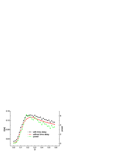
Figure 1: (color online) Stochastic resonance behavior of overdamped bistable system (9) for periodic signal with matched filtering measurement method. Ensemble averaged matched ratio($E[{\cal M}]$ Eq.(11), solid line) and the output signal power (dashed line) are plotted. Both show perfect stochastic resonance behavior. In addition this two results are consistent to each other very well. The line marked with triangle is $E[{\cal M}]$ without time delay. We can see that $E[{\cal M}]$ with and without time delay show the same qualitative behavior. This is because that our template actually has no time delay respect to the output data stream.

IV.2 chirp signal input

Secondly, we set the input signal as the gravitational wave signal radiated from two merging black holes or neutron stars which reads

$$S_{p}(t)=\frac{A}{\sqrt[4]{t_{\text{coal}}-t}}\cos\left[\omega(t_{\text{coal}}-t)\right]^{5/8}.$$ (13)

$A$ and $\omega$ are two parameters determined by the masses of the binary system’s sub-bodies and the distance between the source and the detector. $t_{\text{coal}}$ is the time of coalescence. This wave form is theoretical prediction of post-Newtonian analysis for binary systems which includes black hole-black hole binary, black hole-neutron star binary and neutron star-neutron star binary. In this work we set $A=0.2$, $t_{\text{coal}}=601$ and $\omega=6$. This signal is a typical wideband signal. Our parameters setting makes the frequency band locate around $0.2$. The same to above subsection, the simulation time is $600$ time units which is very near the coalescence time $601$.

Since this signal is not periodic, we have no time scale to guide us to choose the range of time delay $\Delta$ in equation (11). Here we propose to use try error method to find out the true stochastic resonance behavior. Try error method we mean trying different time delay range from small to large till the result converges. Here converge means resulting in the almost same optimal noise intensity. Theoretically the time delay is longer the convergence is better. But the data stream has finite length in practice. These results are plotted in Fig.2. Since our input signal and template has no time delay at all, we expect the line without time delay should be the converged result. But we see a small but nonvanishing difference between different time delays. This is because our data stream is some short, only 600 steps, while different time delay results in different effective length of data array.

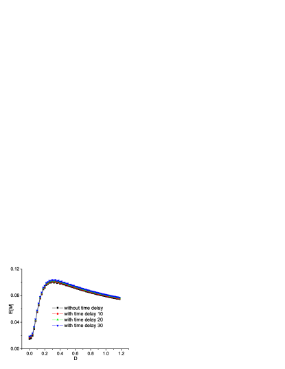
Figure 2: (color online) Stochastic resonance behavior of overdamped bistable system (9) for chirp signal with matched filtering measurement method. The $E[{\cal M}]$ without time delay (marked with square) and with different time delay ($10$ marked with disk, $20$ marked with up triangle and $30$ marked with down triangle) are plotted respectively. All of these lines show well convergence behavior which implies that the one without time delay has already described the true stochastic resonance behavior already. This is consistent with expected result, because our input signal and template has no time delay at all with equation (9).

IV.3 random pulse signal

At last but not at least, we use random pulse signal as the input. We follow hu92 closely to construct the random pulse. Each pulse takes a value

$$S_{p}(t)=A\text{ or }S_{p}(t)=-A$$ (14)

and persists for time $\frac{T}{2}$. Each $A$ or $-A$ are randomly taken with probability $1/2$ respectively. In this work we set $A=0.05$ and $T=\frac{2\pi}{0.2}$. We set simulation time $600$ units still.

Similar to above chirp case, we use try error method to determine the stochastic resonance again. We concluded all these results in Fig.3.

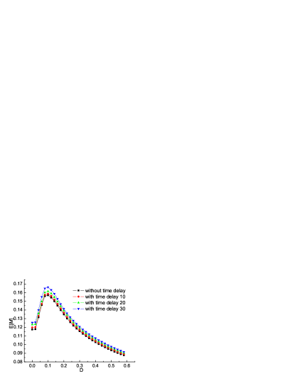
Figure 3: (color online) Stochastic resonance behavior of overdamped bistable system (9) for random pulse input with matched filtering measurement method. This result is very similar with above ones but shows different optimal noise intensity. This is reasonable because of the different driven signal. This figure shows that matched filtering method can also describe non-periodic stochastic resonance very well.

All three figures show that the one without time delay has already described the true stochastic resonance behavior already. This is consistent with expected result, because our input signal and template has no time delay at all with equation (9). But generally, the time delay is important for the stochastic resonance measurement quantity (11) when the template does has time delay compared with the data stream.

V conclusion and discussion

Since 2003 the ground-based interferometric gravitational wave detector Laser Interferometer Gravitational Wave Observatory (LIGO) has taken several real experimental data. And other high sensitive detector such as VIRGO, GEO and TAMA have also achieved their expected sensitivities. At the same time, the space-based interferometric gravitational wave detector LISA is also under way. Along with the development of these high sensitive detector, we are entering into an epoch of gravitational wave astronomy. Gravitational wave detection is a typical example of weak signal detection where stochastic resonance may be applicable. But almost all of the data analysis method in gravitational wave detection are based on matched filtering. In contrast, almost all of the stochastic resonance theory is related to Fourier transformation which does not relate to matched filtering. Here our work do the first step trying to relate matched filtering with stochastic resonance.

The encouraging result of our work is that we do find that the stochastic phenomena emerges with matched filtering data analysis method. And more interestingly, matched filtering method can deal with not only periodic but also non-periodic stochastic resonance. Specifically, we show that matched filtering can deal with stochastic resonance which is driven by sinusoidal signal, which corresponds to periodic gravitational wave; chirp signal, which corresponds to gravitational wave from merging binary system; and random pulse signal. The interesting problem in the following is whether and how to apply our findings and stochastic resonance theory to do gravitational wave data analysis and gravitational wave detector construction.

On the other hand the measurement quantity (11), first proposed in this work, is a novel characteristic measurement for stochastic resonance. Our quantity can not only deal with periodic but also non-periodic stochastic resonance, which improves the conventional Fourier transform method. We hope our new stochastic resonance measurement can find its usage in the future research.

- (1) R. Benzi, A. Sutera, and A. Vulpiani, J. Phys. A 14, L453 (1981); C. Nicolis, Sol. Phys. 74, 473 (1981); C. Nicolis, Tellus 34, 1 (1982).
- (2) L. Gammaitoni, P. Haenggi, P. Jung, F. Marchesoni, Rev. Mod. Phys. 70, 223 (1998); T. Wellens, V. Shatokhin, and A. Buchleitner, Rep. Prog. Phys. 67, 45 (2004) and the references there.
- (3) S. Bezrukov and I. Vodyanoy, Nature (London) 378, 362 (1995); ibid 385, 319 (1997); ibid 386, 738 (1997).
- (4) V. Berdichevsky and M. Gitterman, Europhys. Lett. 36, 161 (1996).
- (5) R. Lofstedt, S. Coppersmith, Phys. Rev. Lett. 72, 1947 (1994); M. Grifoni, P. Hanggi, Phys. Rev. Lett. 76, 1611 (1996); A. Buchleitner, R. Mantegna, Phys. Rev. Lett. 80, 3932 (1998).
- (6) M. Dykman et al., Phys. Rev. Lett. 68, 2985 (1992).
- (7) L. Landau and E. Lifshitz, Physique Statistique (Mir, Moscow, 1984), Sec. 124.
- (8) V. Galdi, V. Pierro, I. Pinto, Gravitational Waves, Second Edoardo Amaldi Conference held in CERN, Switzerland, 1-4 July 1997. Edited by E. Coccia, G. Veneziano, and G. Pizzella. World Scientific, p.532 (1998).
- (9) P. Jung and P. Hanggi, Phys. Rev. A 44, 8032 (1991).
- (10) D. Gong et al., Phys. Rev. A 46, 3243 (1992); 48, 4862(E) (1993).
- (11) M. Inchiosa and A. Bulsara, Phys. Rev. E 52, 327 (1995); ibid 53, R2021 (1996).
- (12) K. Loerincz et al., Phys. Lett. A 224, 63 (1996).
- (13) V. Galdi, V. Pierro, and I. Pinto, Phys. Rev. E 57, 6470 (1998).
- (14) L. Gammaitoni et al., Phys. Lett. A 142, 59 (1989).
- (15) G. Karapetyan, Optics Communications 238, 35 (2004); Phys. Rev. D 73, 122003 (2006).
- (16) K. Thorne, in 300 Years of Gravitation, edited by S. Hawking and W. Israel (Cambridge University Press, Cambridge, England, 1987), pp.330-458.
- (17) C. Cutler and E. Flanagan, Phys. Rev. D 49, 2658 (1994).
- (18) B. Owen and B. Sathyaprakash, Phys. Rev. D 60, 022002 (1999).
- (19) See e.g. S. Babak et al., Classical Quantum Gravity 23, 5477 (2006); S. Babak, H. Grote, M. Hewitson, H. Luck, and K. A. Strain, Phys. Rev. D 72, 022002 (2005); Y. Tsunesada et al., Phys. Rev. D 71, 103005 (2005).
- (20) R. Lofstedt and S. Coppersmith, Phys. Rev. E 49, 4821 (1994).
- (21) C. Heneghan et al, Phys. Rev. E 54, 2228 (1996).
- (22) P. Greenwood et al, Phys. Rev. Lett. 84, 4773 (2000).
- (23) A. Neiman et al, Phys. Rev. Lett. 76, 4299 (1996); I. Goychuk and P. Hanggi, Phys. Rev. E 61, 4272 (2000).
- (24) J. Robinson, D. Asraf, A. Bulsara and M. Inchiosa, Phys. Rev. Lett. 81, 2850 (1998).
- (25) J. Collins, C. Chow and T. Imhoff, Nature (London) 376, 236 (1995); Phys. Rev. E 52, 3321 (1995).
- (26) H. Kantz and T. Schreiber, Nonlinear time series analysis (Cambridge University Press, 1997).
- (27) H. Caulfield, Appl. Opt. 21, 4391 (1982).
- (28) G. Hu, G. Qing, D. Gong and X. Wen, Phys. Rev. A 44, 6414 (1991).
- (29) G. Hu, et al, Phys. Rev. A 46, 3250 (1992).
- (30) See e.g., L. Gammaitoni, F. Marchesoni, E. Menichella-Saetta, and S. Santucci, Phys. Rev. Lett. 62, 349 (1989); L. Gammaitoni, F. Marchesoni, and S. Santucci, Phys. Rev. Lett. 74, 1052 (1995); A. Neiman, L. Schimansky-Geier, Phys. Rev. Lett. 72, 2988 (1994); Y. Jia, S. Yu, and J. Li, Phys. Rev. E 62, 1869 (2000); T. Zhou, F. Moss, and P. Jung, Phys. Rev. A 42, 3161 (1990).
- (31) H. Risken, The Fokker-Planck Equation: Methods of solution and Applications (New York: Springer) (1983).