Scaling with system size of the Lyapunov exponents for the Hamiltonian Mean Field model

Abstract

The Hamiltonian Mean Field (HMF) model is a prototype for systems with long-range interactions. It describes the motion of $N$ particles moving on a ring, coupled through an infinite-range potential. The model has a second order phase transition at the energy density $U_{c}=3/4$ and its dynamics is exactly described by the Vlasov equation in the $N\to\infty$ limit. Its chaotic properties have been investigated in the past, but the determination of the scaling with $N$ of the Lyapunov Spectrum (LS) of the model remains a challenging open problem. We here show that the $N^{-1/3}$ scaling of the Maximal Lyapunov Exponent (MLE), found in previous numerical and analytical studies, extends to the full LS; not only, scaling is “precocious” for the LS, meaning that it becomes manifest for a much smaller number of particles than the one needed to check the scaling for the MLE. Besides that, the $N^{-1/3}$ scaling appears to be valid not only for $U>U_{c}$, as suggested by theoretical approaches based on a random matrix approximation, but also below a threshold energy $U_{t}\approx 0.2$. Using a recently proposed method (GALI) devised to rapidly check the chaotic or regular nature of an orbit, we find that $U_{t}$ is also the energy at which a sharp transition from weak to strong chaos is present in the phase-space of the model. Around this energy the phase of the vector order parameter of the model becomes strongly time dependent, inducing a significant untrapping of particles from a nonlinear resonance.

and

1 Introduction

The dynamical and statistical properties of systems with long-range interactions have recently attracted considerable attention (see Campa et al. (2009) for a recent review). The Hamiltonian Mean Field (HMF) model (Antoni & Ruffo, 1995) is considered as a prototype for some of the observed dynamical effects. The model describes the motion of $N$ fully coupled particles lying on a ring. The system presents a second order phase transition at the critical energy density $U_{c}=E_{c}/N=3/4$ from a low-energy phase, where the particles are clustered, to a high-energy gaseous phase where the particles are uniformly distributed on the ring. Several different effects have been studied for this model, which have been then found to be generic for a large class of systems with long-range interactions, including self-gravitating systems, unscreened plasmas, two-dimensional hydrodynamics, etc..

The question on which we concentrate in this paper is the behavior of the Lyapunov exponents. This question has been investigated for a long time, already in some of the first papers on the HMF model. However, a general understanding of the chaotic properties of this model remains a challenge. Since we will be mostly concerned with the $N\to\infty$ behavior of the Lyapunov exponents, this question has a relevance also for the Vlasov equation, which is known to describe exactly the dynamics of the HMF model in this limit (Campa et al., 2009).

Let us briefly summarize the state of the art knowledge on the Lyapunov exponents for the HMF model. The Maximal Lyapunov Exponent (MLE) increases with energy up to the critical energy density $U_{c}$ and then decreases for larger energies (Yamaguchi, 1996). In the whole high energy phase it drops to zero in the large $N$ limit as $N^{-1/3}$ (Latora et al., 1998). An analytical estimate of the MLE, which takes into account microcanonical averages of suitable geometrical observables (Pettini, 2007), was proposed by Firpo (1998). A preliminary study of the scaling properties of the Lyapunov Spectra (LS) and of the Kolmogorov-Sinai (KS) entropy was performed by Latora et al. (1999). Lyapunov instability of a modified HMF model, the so-called $\alpha$-HMF, was first studied by Anteneodo & Tsallis (1998) and further analyzed by Campa et al. (2001, 2002). The $N^{-1/3}$ scaling has been shown to derive from a random matrix approximation (Firpo & Ruffo, 2001; Anteneodo & Vallejos, 2001; Vallejos & Anteneodo, 2002; Anteneodo et al., 2003). A supersymmetric approach (Tănase-Nicola & Kurchan, 2003) suggests that the MLE might vanish in the $N\to\infty$ for all energies. A tendency of the model towards integrability when $N$ increases, meaning a vanishing MLE, has been recently emphasized using a Poincaré return map approach (Bachelard et al., 2008). Lyapunov exponents and the corresponding eigenmodes of the HMF model have been also recently studied in the Vlasov $N\to\infty$ limit (Paskauskas & De Ninno, 2009).

The aim of this paper is to present a careful assessment of the scaling properties with $N$ of the MLE, the LS and the KS entropy of the HMF model in various energy ranges and in conditions as close as possible to Boltzmann-Gibbs thermal equilibrium. With respect to previous studies, we have put more effort in establishing the equilibrium state, knowing that this is not easily reached due to the presence of quasi-stationary states (Campa et al., 2009). These latter are out–of–equilibrium states in which the system remains trapped for a time that increases with $N$, slowing down indefinitely the relaxation to thermal equilibrium.

An alternative approach, designed for fast detection of chaotic orbits, has been recently proposed (Skokos et al., 2007). The method, which has been called Generalized Alignment Index (GALI), allows one to distinguish between regular and chaotic motion using short-time numerical integrations. The GALI method takes into account more than one deviation vector and measures the time evolution of the volume of the parallelepiped whose edges are these normalized vectors. In this paper we use the GALI method to detect the fraction of chaotic orbits on a constant energy surface of the HMF model.

The paper is organized as follows. In Section 2 we briefly introduce the HMF model and we discuss the main features of the Boltzmann-Gibbs statistical equilibrium state. In Section 3 we recall how the LS is computed, in order to make the paper self-consistent. Afterwards, in Section 4, we present the core results of this paper, by discussing the scaling with $N$ of the MLE, the LS and the KS entropy. In Section 5 we describe the GALI chaos detection method and we test its efficiency by considering the HMF model with a small number of particles. In Section 6 we use the GALI method for the estimation of the fraction of chaotic orbits in the model’s phase space. Our conclusions are finally summarized in Section 7.

2 The HMF model and its statistical equilibrium

The Hamiltonian Mean Field (HMF) model (Antoni & Ruffo, 1995) describes a system of point masses moving on a ring and interacting through an infinite-range potential. The Hamiltonian of the model is

$$H=\sum_{i=1}^{N}\frac{p_{i}^{2}}{2}+\frac{1}{2N}\sum_{i,j=1}^{N}[1-\cos(\theta_{i}-\theta_{j})],$$ (1)

where $\theta_{i}\in(\pi,\pi]$ is the coordinate of the $i$-th particle and $p_{i}$ its conjugate momentum. The system has only two constants of the motion: total energy $H$ and total momentum $\sum_{i}p_{i}$ (in the following we will always choose a zero total momentum without loosing generality). As the force vanishes when $i=j$, the particles do not collide but smoothly cross each other. The order parameter of this model is the “magnetization” vector

$$\mathbf{M}=\frac{1}{N}\sum_{i=1}^{N}(\cos\theta_{i},\sin\theta_{i})=(M_{x},M_{y})~{},$$ (2)

and, after defining its phase $\phi=\arctan M_{y}/M_{x}$ and modulus $M=\sqrt{M_{x}^{2}+M_{y}^{2}}$, the equations of motion can be written as

$$\left\{\begin{array}[]{ll}\dot{\theta}_{i}=p_{i}\\ \dot{p}_{i}=-M_{x}\sin\theta_{i}+M_{y}\cos\theta_{i}=-M\sin(\theta_{i}-\phi)~{}.\end{array}\right.$$ (5)

We solve numerically the equations of motion of the HMF model using an optimized fourth-order symplectic integrator (McLachlan & Atela, 1992) with time step $h=0.05$, which typically gives a relative energy fluctuation $\Delta E/E\sim 10^{-4}$.

The equilibrium statistical mechanics of the HMF model has been thoroughly studied (see Campa et al. (2009) for a review). The model has a second order phase transition at the critical energy density $U_{c}=3/4$ from a low-energy clustered phase where $M\neq 0$ to a high-energy gaseous phase where $M=0$. Being this phase transition of second order, it cannot be associated with a negative specific heat. The canonical and microcanonical ensemble give equivalent results (Campa et al., 2009).

In the mean-field limit, $N\to\infty$, the dynamics of the HMF model is fully described by the single particle distribution function $f(\theta,p,t)$, where $(\theta,p)$ are the canonically conjugate Eulerian coordinates of the single particle phase space. The single particle distribution function obeys a Vlasov equation. Among many stationary solutions of the Vlasov equation, a particular one is the Boltzmann-Gibbs equilibrium distribution

$$f_{eq}(\theta,p)=\frac{\sqrt{\beta}}{(2\pi)^{3/2}I_{0}(\beta M)}\exp[\beta(\frac{p^{2}}{2}-M\cos(\theta-\phi)],$$ (6)

where $\beta=1/T$ is the inverse temperature and $I_{0}$ is the modified Bessel function of order zero. This distribution is also stable with $M=0$ for $\beta\leq\beta_{c}=2$ and with $M\neq 0$ for $\beta>\beta_{c}$. Therefore, $\beta_{c}$ can be interpreted as the inverse critical temperature of the second order phase transition, corresponding to the critical energy $U_{c}$.

In order to reach the equilibrium distribution (6) on a reasonably short time scale, we have initialized positions with a Gaussian distribution and we have computed the corresponding potential energy. We then determined the appropriate width of the Gaussian distribution of momenta which gave the energy we wanted to achieve. This initial state was then evolved for a long time in order for the equilibrium distribution of Eq. (6) to be reproduced with a sufficient precision. For instance, for the $N=100$ particle case, we can reproduce the equilibrium temperature with a relative error of a few percent, which is compatible with the statistical error, expected to be of the order $N^{-1/2}$.

3 The Lyapunov spectrum

For the sake of completeness, we briefly recall how the Lyapunov spectrum of a $2N$-dimensional flow is defined and computed (Benettin et al., 1980a, b), with reference to the HMF model.

The $2N$-dimensional phase-space coordinate is

$$\mathbf{x}\equiv\left(\theta_{1},\dots,\theta_{N},p_{1},\dots,p_{N}\right)$$ (7)

and the phase-space flow is generated by the system of autonomous first-order differential equations (5), which, using $\mathbf{x}$, can be written as

$$\frac{d\mathbf{x}(t)}{dt}=F(\mathbf{x}(t))~{},$$ (8)

where $F$ is the velocity field of the flow.

The evolution equations for the deviation vector

$$\mathbf{w}\equiv\left(\delta\theta_{1},\dots,\delta\theta_{N},\delta p_{1},\dots,\delta p_{N}\right)$$ (9)

are

$$\frac{d\mathbf{w}}{dt}=\tilde{J}(\mathbf{x}(t))\mathbf{w}~{},$$ (10)

where the $2N\times 2N$ Jacobian matrix of the flow $\tilde{J}(\mathbf{x}(t))=\partial F/\partial\mathbf{x}$ is given by

$$\tilde{J}=\left(\begin{array}[]{cc}0&I\\ J&0\\ \end{array}\right)~{},$$ (11)

with the $N\times N$ Jacobian $J_{ij}=-\partial^{2}V/\partial\theta_{i}\partial\theta_{j}$ given by

$$\left\{\begin{array}[]{ll}J_{ii}=-\cos(\theta_{i})M_{x}-\sin(\theta_{i})M_{y}+\frac{1}{N}\\ J_{ij}=\frac{1}{N}\cos(\theta_{i}-\theta_{j}),\quad\text{if}\quad i\neq j~{},\end{array}\right.$$ (14)

and $I$ the $N\times N$ identity matrix.

The linear evolution equations (10) are integrated with initial value $\mathbf{w}(0)$, which physically represents the “small” initial difference between two nearby orbits of Eq. (8). Numerically, this integration is performed in parallel with that of the orbit $\mathbf{x}(t)$, since $\tilde{J}$ depends on it. One typically uses the same integration algorithm.

The Maximal Lyapunov Exponent (MLE) is then defined as

$$\lambda(\mathbf{x}(0))=\lim_{t\rightarrow\infty}\frac{1}{t}\ln\frac{\|\mathbf{w}(t)\|}{\|\mathbf{w}(0)\|}.$$ (15)

Practically, since $\|\mathbf{w}(t)\|$ diverges exponentially, one has to renormalize it at regular time intervals. The computation of the MLE is performed by averaging the renormalization factors.

Furthermore, when varying $\|\mathbf{w}(0)\|$, one can obtain at most $2N$ Lyapunov exponents, which can be ordered in size

$$\lambda_{1}\geq\lambda_{2}...\geq\lambda_{2N}~{},$$ (16)

and constitute the so-called Lyapunov Spectrum (LS), with $\lambda_{1}=\lambda(\mathbf{x}(0))$.

For Hamiltonian flows, the LS is endowed of the following symmetry property

$$\lambda_{i}=-\lambda_{2N-i+1},\quad i=1,2,...,2N~{}.$$ (17)

It is then enough to compute the first $N$ exponents. Among them, for the HMF model, two are zero because of energy and momentum conservation. For a chaotic orbit all the others are typically positive.

However, because of the numerical instability which tends to align the deviation vector $\mathbf{w}(t)$ along the most expanding direction, one always obtains $\lambda_{1}$ and has not access to the full LS.

The trick to perform numerically the calculation of the full LS was found by Benettin et al. (1980a, b) and amounts to compute the hypervolume

$$\mathcal{V}_{p}(t)=\mathbf{w}_{1}(t)\wedge\mathbf{w}_{2}(t)\wedge...\wedge\mathbf{w}_{p}(t),$$ (18)

for $p$ deviation vectors $\mathbf{w}_{1}(t),...,\mathbf{w}_{p}(t)$.

Then, the sum of the first $p$ Lyapunov exponents

$$\lambda^{(p)}=\lambda_{1}+\lambda_{2}+...+\lambda_{p}$$ (19)

is given by

$$\lambda^{(p)}(\mathbf{x}(0))=\lim_{t\rightarrow\infty}\frac{1}{t}\ln\frac{\|\mathcal{V}_{p}(t)\|}{\|\mathcal{V}_{p}(0)\|}~{}.$$ (20)

A recent review about the Lyapunov exponents and their calculation can be found in Skokos (2010).

Once the LS is known, the Kolmogorov-Sinai (KS) entropy, which is the rate of information production, is given by

$$S_{KS}=\sum_{i=1}^{N}\lambda_{i}~{}.$$ (21)

4 Scaling with $N$ of the MLE, the LS and the KS entropy

As mentioned in the Introduction, it has been proposed that in the whole high energy region $U\geq U_{c}$ the MLE should vanish as $N^{-1/3}$. We want to show here that this scaling law is obeyed also by the full LS.

In panels a) and c) of Fig. 1 we plot $\lambda_{i}$ vs. $i/N$, increasing $N$ from $N=50$ to $N=500$, for $U=0.1$ (panel a) and $U=1.2$ (panel c). The total integration time was $0.5\times 10^{6}$ with time step $h=0.05$, which provides a good convergence for the LS and a good accuracy for the energy conservation as well. The relative error in the determination of the MLE is of the order of $1\%$. We observe a general decreasing trend, showing a significant size dependence of the LS. This size dependence is almost completely eliminated when multiplying the LS by $N^{1/3}$, as shown in panels b) and d) of the same figure. We observe a reasonably good “data collapse” in the upper and lower parts of the spectrum. However, the insets in panels b) and d) show that the size dependence is not yet completely eliminated and remains of the order of $10\%$. The insets reveal another interesting feature: while the convergence to an asymptotic LS is from above for the full LS at $U=0.1$, at the energy $U=1.2$ it is from above only for the largest exponents and it is instead from below for the smaller exponents.

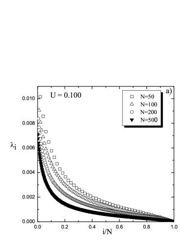
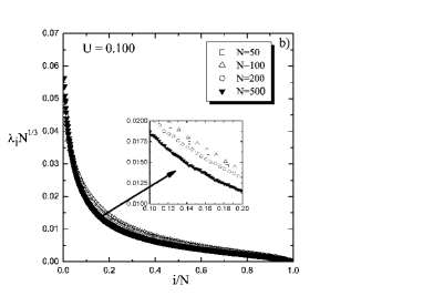
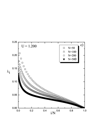
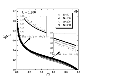
Figure 1: LS vs. $i/N$ for $U=0.1$ (panel a) and $U=1.2$ (panel c). For the same energies we also show the LS multiplied by $N^{1/3}$ (panels b and d). The insets show details of the size dependence with more resolution.

In Fig. 2 we show the $N$ dependence of $\lambda_{1}$ for $U=0.1$, which is well fitted by the scaling law $N^{-1/3}$, confirming the result obtained by looking at the full LS. However, one has to reach much larger system sizes (of the order of $10^{6}$) in order to check the scaling law, while the convergence to the asymptotic LS as $N$ increases is observed for much smaller system sizes (up to $N=500$).

Other numerical experiments (Latora et al., 1998; Anteneodo & Tsallis, 1998; Anteneodo et al., 2003) show that this scaling law is present also for energies above $U_{c}$, but the quality of the data is never comparable with the one obtained here for $U=0.1$.

While the scaling in the high energy range can be justified using a random matrix approximation (Latora et al., 1998; Anteneodo & Tsallis, 1998; Anteneodo & Vallejos, 2001) and a theory using geometric properties of the phase-space (Pettini, 2007; Firpo, 1998), no theoretical approach exists for the explanation of the $N^{-1/3}$ scaling at low energies. On the other hand, the only theoretical approach valid in this energy region (Firpo, 1998) would predict a strictly positive MLE in the $N\to\infty$ limit.

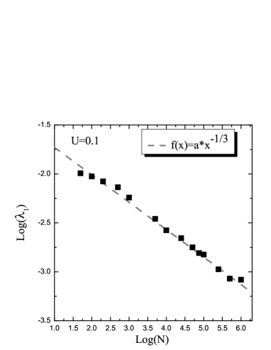
Figure 2: Logarithm of the MLE vs. $\log N$ for $U=0.1$, showing the $N^{-1/3}$ scaling. Both logarithms are in base $10$.

In Fig. 3a), we show the MLE as a function of $U$ for various system sizes: $N=50,100,200,500$. One observes a sharp increase of the MLE around the energy $U_{t}\approx 0.2$. We’ll come back to comment about this energy value in Section 6. The MLE is peaked around the critical energy $U_{c}$ and shows, in this range of sizes, a weak size dependence for $U<U_{c}$ while for $U>U_{c}$ it systematically and monotonically decreases with system size. In panel b) of the same figure, we check if the $N^{-1/3}$ scaling found for the LS works also for the MLE, by multiplying all MLE by the factor $N^{1/3}$. It turns out that this scaling does not work well for this relatively small number of particles. An “indermediate” scaling with a factor $N^{-1/4}$ looks slightly better in the high energy range, see Fig. 3c.

As a partial conclusion, we could state that the MLE shows a size dependence over the whole energy range, but the $N^{-1/3}$ scaling does not emerge easily from the data. This is at variance with the analysis above of the LS, for which this scaling was more evident. This is why we speak of “precocious” scaling of the LS, meaning that the scaling is obtained for moderately large system sizes, while the scaling of the MLE, as shown e.g. in Fig. 2, needs much larger systems sizes to be numerically emphasized.

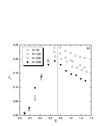
Figure 3: a) The MLE, $\lambda_{1}$, as a function of $U$ for various system sizes $N=50,100,200,500$ (the vertical line shows the critical energy $U_{c}=3/4$). b) MLE multiplied by the factor $N^{1/3}$ vs. $U$. c) MLE multiplied by the factor $N^{1/4}$ vs. $U$.

Since the KS entropy is the sum of all positive Lyapunov exponents, inheriting some features of the LS, we expect that the scaling should be revealed more easily. This is indeed the case, as shown in Fig. 4, where we plot the KS entropy density $S_{KS}/N$ vs. $U$ for several system sizes (panel a) and the same quantity multiplied either by $N^{1/3}$ (panel b) or by $N^{1/4}$ (panel c). From panel a) we observe that the KS entropy shows a general trend to decrease for all energies, as the system size increases. This is more evident than for the MLE. Panel b) shows that this size dependence is almost completely eliminated for $U<U_{c}$, hence the $N^{-1/3}$ factor captures some essential feature of the scaling for all energies. However, in the $U>U_{c}$ range we still observe a significant size dependence. This latter is almost completely eliminated in panel c), where we multiply the KS entropy by $N^{1/4}$, a phenomenological factor for which we have no theoretical justification. The low energy KS entropy scaling is however spoiled by this rescaling, showing that a global scaling, valid for all energies, does not seem to exist. It is also clear that the KS entropy peak is shifted at energies larger than $U_{c}$, at variance with the behavior of the MLE.

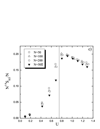
Figure 4: a) KS entropy density vs. energy $U$ for the same data and system sizes as in Fig. 3. b) KS entropy density vs. $U$ multiplied by the factor $N^{1/3}$. c) KS entropy density vs. $U$ multiplied by the factor $N^{1/4}$.

The dependence of the MLE on system size will be investigated in more detail in Leoncini et al. (2010), going to number of particles of the order of $N=10^{6}$.

5 The GALI indices

In this Section we will briefly introduce the definition of the Generalized Alignment Indices (GALI) (Skokos et al., 2007) and we will comment on their physical meaning and their relation with Lyapunov exponents. We will also present the application of the method to the HMF model with a limited number of particles, to show its efficiency for the fast detection of chaotic orbits.

The GALI index of order $p$ (GALI_p) is determined through the evolution of $2\leq p\leq 2N$ initially linearly independent deviation vectors $\textbf{w}_{i}(0),i=1,2,...,p$. Its calculation is therefore strongly related to the one of the LS. The evolved deviation vectors $\textbf{w}_{i}(t)$ are normalized at given time intervals in order to avoid overflows, but their directions are kept unchanged. Then, according to Skokos et al. (2007), GALI_p is defined to be the volume of the $p$-parallelogram having as edges the $p$ unit deviation vectors $\hat{\textbf{w}}_{i}(t)=\textbf{w}_{i}(t)/\|\textbf{w}_{i}(t)\|,i=1,2,...,p$

$$\text{GALI}_{p}(t)=\parallel\hat{\textbf{w}}_{1}(t)\wedge\hat{\textbf{w}}_{2}(t)\wedge...\wedge\hat{\textbf{w}}_{p}(t)\parallel.$$ (22)

From this definition it is evident that if at least two of the deviation vectors become linearly dependent during dynamical evolution, the wedge product in Eq. (22) becomes zero and the GALI_p vanishes.

In the case of a chaotic orbit, all deviation vectors tend to become linearly dependent, aligning along the eigenvector corresponding to the maximal Lyapunov exponent and GALI_p tends exponentially to zero following the law (Skokos et al., 2007)

$$\text{GALI}_{p}(t)\sim e^{-[(\lambda_{1}-\lambda_{2})+(\lambda_{1}-\lambda_{3})+...+(\lambda_{1}-\lambda_{p})]t},$$ (23)

where the $\lambda_{i}$ are the Lyapunov exponents (or, better, their finite time approximations).

In the case of regular motion, all deviation vectors move on the $N$-dimensional tangent space of a torus, on which the motion is quasiperiodic. Thus, if one starts with $p\leq N$ deviation vectors, these will remain linearly independent on this tangent space, since there is no particular reason for them to become aligned. As a consequence, GALI_p remains in this case practically constant for all $p\leq N$. On the other hand, for $p>N$, GALI_p tends to zero, since some deviation vector will eventually become linearly dependent. According to Christodoulidi & Bountis (2006); Skokos et al. (2008), the GALI indices associated with a quasiperiodic orbit lying on a $m$-dimensional torus (with $m<N$) behave as follows

$$\text{GALI}_{p}(t)\sim\left\{\begin{array}[]{ll}\text{constant},&\hbox{if $2\leq p\leq m$}\\ \frac{1}{t^{p-m}},&\hbox{if $m<p\leq 2N-m$}\\ \frac{1}{t^{2(p-N)}},&\hbox{if $2N-m<p\leq 2N$}.\end{array}\right.$$ (24)

When $m=N$, GALI_p remains constant for $2\leq p\leq N$ and decreases to zero as $\sim 1/t^{2(p-N)}$ for $N<p\leq 2N$. An efficient way to calculate GALI_p is by multiplying the singular values $z_{i},i=1,...,p$, computed using the singular value decomposition procedure of the matrix formed by the deviation vectors $\hat{\textbf{w}}_{i},i=1,...,p$ (Antonopoulos & Bountis, 2006; Skokos et al., 2008)

$$\text{GALI}_{p}=\prod_{i=1}^{p}z_{i}.$$ (25)

The method has been applied successfully to several Hamiltonian systems like the FPU lattice (Skokos et al., 2008) and to coupled symplectic maps (Bountis et al., 2009). It has been shown that it efficiently detects not only regular and chaotic motion but also the dimensionality of the tori on which the regular trajectory lies.

We begin by analyzing the GALI indices for systems with a few particles and we show examples of computations performed for the HMF model with $N=2$ (integrable case) and $N=3$.

For $N=2$ we have access to GALI_2,3,4, since in this case the dimension of the phase space is $2N=4$. Besides energy, also total momentum is conserved; hence the system is integrable and the motion is expected to be regular for all energies. Following the definition of the GALI indices for regular motion, Eq. (24), we should expect

$$\text{GALI}_{2}(t) \propto\text{const.},\quad\text{GALI}_{3}(t)\propto\frac{1}{t^{2}},\quad\text{GALI}_{4}(t)\propto\frac{1}{t^{4}}.$$ (26)

Indeed, choosing an initial condition with $U=0.35$ and integrating it up to $t=10^{6}$, we see in panel a) of Fig. 5 that it produces exactly the predicted time evolution for the GALI_2,3,4.

For $N=3$ we detect both regular motion (Fig. 5b for $U=0.07$ and Fig. 5d for $U=1.7$) and chaotic motion (Fig. 5c for $U=0.51$). In the regular case GALI_2,3 stay constant, implying a motion that lies on a 3 dimensional torus while GALI_4,5,6 decay following the power laws

$$\text{GALI}_{4}(t)\propto\frac{1}{t^{2}},\qquad\text{GALI}_{5}(t)\propto\frac{1}{t^{4}},\qquad\text{GALI}_{6}(t)\propto\frac{1}{t^{6}}.$$ (27)

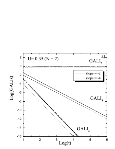
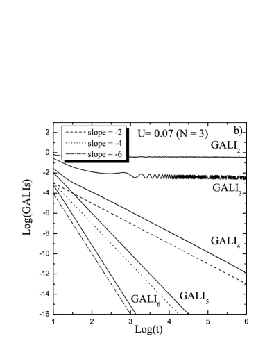
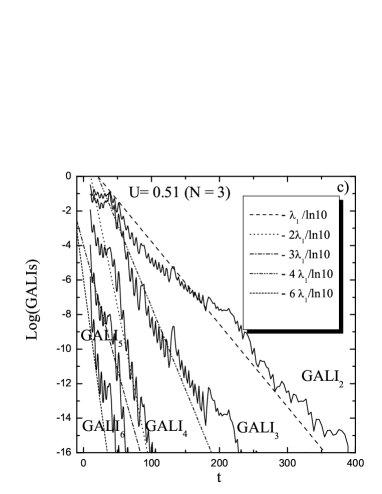
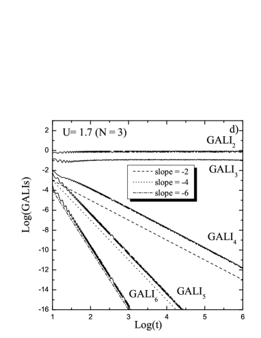
Figure 5: GALI indices vs. time for regular and chaotic orbits. a) HMF model with $N=2$ and energy $U=0.35$: integrable system for which GALI_3,4 decay to zero with the power law predicted theoretically. b) HMF model with $N=3$ and energy $U=0.07$ for which GALI_2,3 are constant: the motion lies on a 3 dimensional torus. c) HMF model with $N=3$ and energy $U=0.51$: chaotic motion is detected, i.e. all GALI’s decay exponentially to zero. The slopes are given by the Lyapunov exponents. d) HMF model with $N=3$ and energy $U=1.7$: the motion is regular and lies again on a 3-dimensional torus.

Chaotic orbits of 3-dimensional Hamiltonian systems generally have two positive Lyapunov exponents. However, in the HMF model also total momentum is conserved and, therefore, only one positive exponent $\lambda_{1}$ is present in the spectrum. Furthermore, due to the symmetry of the Lyapunov spectrum $\lambda_{6}=-\lambda_{1}$. Therefore, according to formula (23), the exponential decay in time of the GALI indices is controlled only by $\lambda_{1}$, as shown in Fig. 5c.

The most important advantage of the GALI method relies on the fact that, for chaotic orbits, the GALI indices decay to zero exponentially fast. Practically, an orbit can be labeled as chaotic when some GALI_p (where $p$ is conveniently chosen) is found to be smaller than a given threshold. This often happens before the MLE stabilizes on an average positive value, making the GALI_p test more efficient in determining chaotic properties of an orbit than the measurement of the MLE. We will give an explicit example of this property of the GALI indices in the next Section.

6 Application of the GALI method to the HMF model with large $N$: the transition from weak to strong chaos

In this Section we will present the application of the GALI method to the HMF model, as a tool to reveal the fraction of chaotic orbits on a constant energy surface with many degrees of freedom. The dependence of such a fraction on the number of degrees of freedom has been recently analyzed for fully or partially connected symplectic maps in Laveder et al. (2008), with an application also to the HMF model.

As we have discussed in the previous Section, the GALI method can be faster in revealing the chaotic or regular nature of a given orbit than the calculation of the MLE. In order to perform a systematic analysis, it is necessary to fix some criteria. The first important choice is the value of $p$ for the GALI_p. In systems with many degrees of freedom we have access to high values of $p$, but the calculation of the corresponding GALI_p would be extremely heavy, since we would have to perform the singular value decomposition for large matrices. Therefore, we are limited ourselves to small values of $p$. We have avoided to use GALI₂, since it has been shown in Skokos et al. (2007) that, for some chaotic orbits of many degrees of freedom systems, the two largest Lyapunov exponents can take very close values. In such chaotic cases, the GALI₂, instead of decreasing exponentially, stays constant, detecting a “false” regular orbit. For the HMF model, in the energy range $0<U<0.4$, we have checked the different time evolution of GALI_3,4,5 and we have finally decided to concentrate our attention on the behavior of GALI₃. Fixing the total integration time to $t=3\times 10^{3}$, we have labeled an orbit as regular if GALI₃ stays above $10^{-4}$ over the whole time lapse. We instead label an orbit as chaotic if GALI₃ goes below $10^{-12}$ within the total integration time. Orbits not satisfying any of these two criteria are analyzed on a longer time span to assess their chaotic or regular nature; however, in the simulations we have performed very few such cases happened. We have decided to fix the number of initial conditions to $1000$ and we have performed simulations with increasing number of particles: $N=100,1000,5000$.

In Fig. 6 we show the fraction of chaotic orbits in $\%$ as a function of $U$. A sharp increase of this fraction is observed around the energy $U_{t}\approx 0.2$. A more quantitative fit to the data for $N=1000$ with the function $f(x)=\alpha*[1+\tanh(\gamma*(U-U_{t}))]$ gives the more precise estimate $U_{t}=0.217...$ (the other fitting parameters being $\alpha=50$ and $\gamma=30$). A significant shift of the transition towards smaller values of $U$ is observed as $N$ is increased. However, it is likely that the curve will reach an asymptotic limit as $N$ is increased (currently not accessible for our computers), since the shift observed when passing from $N=100$ to $N=1000$ (a factor of 10) is of the same order as the one found when further multiplying $N$ by a factor of 5. Moreover, the fraction of chaotic orbits is below $1\%$ for $U<0.15$ and around $99\%$ for $U>0.25$ for all simulated system sizes, showing that a sharp transition from a weakly chaotic to a strongly chaotic phase-space takes place in the energy range $[0.15,0.25]$.

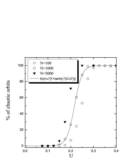
Figure 6: Fraction of chaotic orbits vs. energy $U$ for a different number of particles $N=100,1000,5000$. We also show a fit to the points with $N=1000$ particles (full line). The transition energy from weak to strong chaos is around $U_{t}\approx 0.2$.

It has been suggested by Antoni & Ruffo (1995) that, around energy $0.2$, the phase $\phi$ of the order parameter $\mathbf{M}$ of the HMF model begins to be strongly time dependent, while for smaller energies it is essentially time independent. This determines the untrapping of some particle trajectories from the nonlinear resonance in the pendulum phase-space associated to the model. Since we here find a significant growth of the fraction of chaotic orbits just in this energy range, we wanted to verify the correspondence between the two phenomena.

In Fig. 7 (upper row) we plot the time evolution of GALI₃ for three different energies: $U=0.075,0.2,0.4$. At low energy (panel a) the GALI₃ remains constant, revealing a regular orbit, while at high energy (panel c) it decreases exponentially fast, detecting a chaotic orbit. In the energy region around $U_{t}$, part of the orbits are chaotic and part are regular. We here show (panel b), two orbits that, according to our criteria, are labeled as chaotic (thick full line) and regular (thin full line). In the inset of panel b) we plot the time evolution of the MLE for these two orbits: the MLE of the chaotic orbit is larger that the one of the “regular” orbit, but on this time scale, they are still far from convergence. This proves that the GALI₃ is able to detect the regular and chaotic nature of the orbit faster than the MLE.

Phase motion is absent for the regular orbit at low energy, see Fig. 7d, while it’s clearly present for the chaotic orbit at the highest energy in Fig. 7f. At the energy $U=0.2$ (Fig. 7e) both the chaotic and the regular orbit display phase motion but, surprisingly, the regular orbit shows a “ballistic” motion of the phase. It’s unclear why this happens; a possible explanation is that, for this orbit, untrapped particles remain out of resonance for a longer time. This would imply less chaoticity because some particles remain far from the most chaotic part of the phase-space, which is around the chaotic layer of the separatrix.

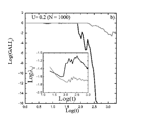
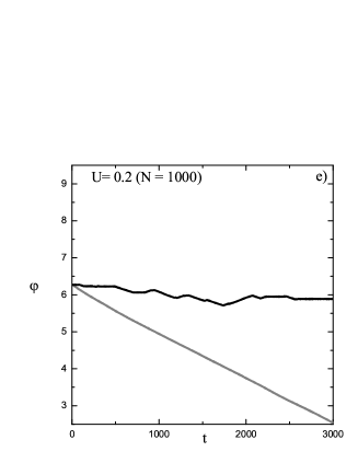
Figure 7: GALI₃ vs. time (upper row) and phase $\phi$ of the order parameter $\mathbf{M}$ (see Eq. 2) vs. time (lower row) at increasing energies for $N=1000$. a) GALI₃ remains constant in time for a regular orbit at $U=0.075$. b) GALI₃ for a chaotic orbit (thick full line) and for a less chaotic one, classified as regular according to our criterion (thin full line), at $U=0.2$. In the inset we show the corresponding time evolution of the MLE. c) GALI₃ decays exponentially for a typical chaotic orbit at $U=0.4$. d) Phase $\phi$ of the order parameter vs. time for $U=0.075$ computed for the orbit of panel a). e) Phase $\phi$ of the order parameter vs. time for $U=0.2$ computed for the two orbits of panel b). f) Phase $\phi$ of the order parameter vs. time for $U=0.4$ computed for the chaotic orbit of panel c).

Although the understanding of the transition from weak to strong chaos appearing around the energy $U_{t}$ is far from being satisfactory, its numerical evidence is clear. Moreover, this threshold energy separates an energy region, $0<U<U_{t}$, where the $N^{-1/3}$ scaling of the MLE and of the LS is clearly found from a higher energy region, $U_{t}<U<U_{c}$, where this scaling is not found with the same evidence. Indeed, in this intermediate energy range, the MLE hardly converges to zero as the system size is increased, as shown in Fig. 3a.

7 Conclusions

Although the chaotic properties of the Hamiltonian Mean Field (HMF) model have been studied in several papers, a general understanding of the behavior of the Lyapunov exponents as the system size is increased and for different energies is still lacking.

We have here shown that, rather than concentrating on the Maximal Lyapunov Exponent (MLE), it is sometimes preferable to determine the full Lyapunov Spectrum (LS). This is certainly more challenging from the numerical point of view, but can be rewarding and reserve some pleasant surprises. We here show, for instance, that the convergence of the LS to its asymptotic, large $N$, shape is more rapid than the one of the MLE.

Moreover, by the study of the LS, the general scaling law with $N^{-1/3}$, originally proposed by Latora et al. (1998), is here found for moderate system sizes. Although this law was originally proposed for the high energy phase of the HMF, above the critical energy $U_{c}=3/4$, we show in this paper that it is also valid in a wide range of low energies, below $U_{t}\approx 0.2$.

With the aim of investigating the physical meaning of this threshold energy $U_{t}$, we have used the newly proposed GALI method by Skokos et al. (2007) in order to determine the fraction of chaotic orbits in the phase-space of the HMF model. The method reveals that this fraction sharply changes from few percents to almost $100\%$ in an energy range around $U_{t}$, showing a transition from weak to strong chaos in this energy region. It is for energies $0<U<U_{t}$ that the $N^{-1/3}$ law is best verified. On the contrary, when $U_{t}<U<U_{c}$, the scaling law is numerically unclear and the MLE shows a slow decrease to zero as the system size increases, which could even lead to suspect that the MLE remains positive in the $N\to\infty$ limit.

Above $U_{c}$ one observes a general trend to decrease to zero of the full LS. The scaling is precocious if one studies full the LS and is again well fitted by the $N^{-1/3}$ law. The MLE also decreases to zero, but with an intermediate scaling with $N^{-1/4}$. It is only for much larger system sizes, of the order of $N=10^{6}$, that one finally finds the $N^{-1/3}$ law also for the MLE.

On the theoretical side, the only existing approach valid in principle for all energies (Firpo, 1998) predicts a strictly positive MLE for $0<U<U_{c}$, while the MLE should vanish as $N^{-1/3}$ for $U>U_{c}$. This is not what we find for $0<U<U_{t}$, demanding for an improvement of this theoretical approach. In the high energy region $U>U_{c}$, a random matrix approximation (Latora et al., 1998; Firpo & Ruffo, 2001; Anteneodo & Vallejos, 2001; Vallejos & Anteneodo, 2002; Anteneodo et al., 2003) predicts the $N^{-1/3}$ scaling of the MLE, which has been checked numerically by Latora et al. (1998); Anteneodo & Tsallis (1998); Anteneodo et al. (2003). It is hard to believe that such an approach could be used for the energy range $0<U<U_{t}$, where the phase-space is mostly occupied by regular orbits, as the GALI method allowed us to assess. The understanding of why the $N^{-1/3}$ scaling is valid in this energy region remains a challenge for future research.

8 Acknowledgements

We would like to thank H. Chaté, D. Fanelli, F. Ginelli, X. Leoncini, R. Paskauskas, A. Politi and Ch. Skokos for fruitful comments and discussions. We acknowledge financial support of the COFIN-PRIN program “Statistical physics of strongly correlated systems at and out of equilibrium” of the Italian MIUR.

References

- Anteneodo & Tsallis (1998) Anteneodo, C., Tsallis, C. (1998). Breakdown of exponential sensitivity to initial conditions: Role of the range of interactions. Phys. Rev. Lett. 80(24):5313-5316.
- Anteneodo & Vallejos (2001) Anteneodo, C., Vallejos, R.O. (2001). Scaling laws for the largest Lyapunov exponent in long-range systems: A random matrix approach. Phys. Rev. E 65:016210.
- Anteneodo et al. (2003) Anteneodo, C., Maia, R. N., Vallejos, R.O. (2003). Lyapunov exponent of many-particle systems: Testing the stochastic approach. Phys. Rev. E 68(3):036120.
- Antoni & Ruffo (1995) Antoni, M., Ruffo, S. (1995). Clustering and relaxation in Hamiltonian long-range dynamics. Phys. Rev. E 52(3):2361-2374.
- Antonopoulos & Bountis (2006) Antonopoulos, Ch., Bountis, T. (2006). Detecting order and chaos by the linear dependence index. ROMAI Journal 2(2):1-13.
- Bachelard et al. (2008) Bachelard, R., Chandre, C., Fanelli, D., Leoncini, X., Ruffo, S., (2008). Abundance of regular orbits and out-of-equilibrium phase transitions. Phys.Rev. Lett. 101:260603.
- Benettin et al. (1980a) Benettin, G., Galgani, L., Giorgilli, A., Strelcyn, J.-M. (1980). Lyapunov characteristic exponents for smooth dynamical systems and for Hamiltonian systems - A method for computing all of them. I: Theory. Meccanica, 9-20.
- Benettin et al. (1980b) Benettin, G., Galgani, L., Giorgilli, A., Strelcyn, J.-M. (1980). Lyapunov characteristic exponents for smooth dynamical systems and for Hamiltonian systems - A method for computing all of them. II: Numerical application. Meccanica, 21-30.
- Bountis et al. (2009) Bountis, T., Manos, T., Christodoulidi, H. (2009). Application of the GALI method to localization dynamics in nonlinear systems. J. Comp. Appl. Math. 227:17-26.
- Campa et al. (2001) Campa, A., Giansanti, A., Moroni, D., Tsallis, C. (2001). Classical spin systems with long-range interactions: universal reduction of mixing. Physics Letters A 286(4):251-256.
- Campa et al. (2002) Campa, A., Giansanti, A., Moroni, D. (2002). Metastable states in a class of long-range Hamiltonian systems. Physica A 305(1-2):137-143.
- Campa et al. (2009) Campa, A., Dauxois, T., Ruffo, S. (2009). Statistical mechanics and dynamics of solvable models with long-range interactions. Phys. Rep. 480:57-159.
- Christodoulidi & Bountis (2006) Christodoulidi, H., Bountis, T. (2006). Low-dimensional quasiperiodic motion in Hamiltonian systems. ROMAI Journal 2(2):37-44.
- Firpo (1998) Firpo, M.C. (1998). Analytic estimation of the Lyapunov exponent in a mean-field model undergoing a phase transition. Phys. Rev. E 57(6):6599-6603.
- Firpo & Ruffo (2001) Firpo, M.C., Ruffo, S. (2001). Chaos suppression in the large size limit for long-range systems. J. Phys. A 34:L511-L518.
- Latora et al. (1998) Latora, V., Rapisarda, A., Ruffo, S. (1998). Lyapunov instability and finite size effects in a system with long-range forces. Phys. Rev. Lett. 80(4):692-695.
- Latora et al. (1999) Latora, V., Rapisarda, A., Ruffo, S. (1999). Chaos and statistical mechanics in the Hamiltonian mean field model. Physica D 131:38-54.
- Laveder et al. (2008) Laveder D., Cosentino M., Lega E., Froeschlé C. (2008). Connectance and stability of nonlinear symplectic systems. Celest. Mech. Dyn. Astr. 102:3-12.
- Leoncini et al. (2010) Leoncini, X., Manos, T., Ruffo, S. (2010). Weak decay of Lyapunov exponent with system size in the -Hamiltonian Mean Field model near equilibrium, (in preparation).
- McLachlan & Atela (1992) McLachlan, R. I., Atela, P. (1992). The accuracy of symplectic integrators. Nonlinearity 5(2):541-562.
- Paskauskas & De Ninno (2009) Paskauskas, R., De Ninno, G. (2009). Lyapunov stability of Vlasov equilibria using Fourier-Hermite modes. Phys. Rev. E 80:036402.
- Pettini (2007) Pettini M. (2007). Geometry and topology in Hamiltonian dynamics and statistical mechanics. Berlin: Springer Verlag.
- Skokos et al. (2007) Skokos, Ch., Bountis, T., Antonopoulos, Ch. (2007). Geometrical properties of local dynamics in Hamiltonian systems: The Generalized Alignment Index (GALI) method. Physica D 231:30-54.
- Skokos et al. (2008) Skokos, Ch., Bountis, T., Antonopoulos, Ch. (2008). Detecting chaos, determining the dimensions of tori and predicting slow diffusion in Fermi-Pasta-Ulam lattices by the Generalized Alignment Index method. Eur. Phys. J. Sp. Top. 165:5-14.
- Skokos (2010) Skokos, Ch. (2010). The Lyapunov characteristic exponents and their computation. Lect. Notes Phys. 790:63-135.
- Tănase-Nicola & Kurchan (2003) Tănase-Nicola, S., Kurchan, J. (2003). Statistical-mechanical formulation of Lyapunov exponents J. Phys. A: Math. Gen. 36(41):10299-10324.
- Vallejos & Anteneodo (2002) Vallejos, R.O., Anteneodo, C. (2002). Theoretical estimates for the largest Lyapunov exponent of many-particle systems. Phys. Rev. E 66(2):021110.
- Yamaguchi (1996) Yamaguchi, Y.Y. (1996). Slow Relaxation at Critical Point of Second Order Phase Transition in a Highly Chaotic Hamiltonian System. Prog. Theor. Phys. 95(4):717-731.