Global Forces in Eruptive Solar Flares: The Lorentz Force Acting on the Solar Atmosphere and the Solar Interior

Abstract

We compute the change in the Lorentz force integrated over the outer solar atmosphere implied by observed changes in vector magnetograms that occur during large, eruptive solar flares. This force perturbation should be balanced by an equal and opposite force perturbation acting on the solar photosphere and solar interior. The resulting expression for the estimated force change in the solar interior generalizes the earlier expression presented by Hudson, Fisher, and Welsch (Astron. Soc. Pac., CS-383, 221, 2008), providing horizontal as well as vertical force components, and provides a more accurate result for the vertical component of the perturbed force. We show that magnetic eruptions should result in the magnetic field at the photosphere becoming more horizontal, and hence should result in a downward (towards the solar interior) force change acting on the photosphere and solar interior, as recently argued from an analysis of magnetogram data by Wang and Liu (Astrophys. J. Lett. 716, L195, 2010). We suggest the existence of an observational relationship between the force change computed from changes in the vector magnetograms, the outward momentum carried by the ejecta from the flare, and the properties of the helioseismic disturbance driven by the downward force change. We use the impulse driven by the Lorentz-force change in the outer solar atmosphere to derive an upper limit to the mass of erupting plasma that can escape from the Sun. Finally, we compare the expected Lorentz-force change at the photosphere with simple estimates from flare-driven gasdynamic disturbances and from an estimate of the perturbed pressure from radiative backwarming of the photosphere in flaring conditions.

1 Introduction

Introduction

Eruptive flares and CMEs result from global reconfigurations of the magnetic-field in the solar atmosphere. Recently, signatures of this magnetic field change have been detected in both vector and line-of-sight magnetograms, the maps of the vector and the line-of-sight component of the photospheric magnetic field, respectively. Is there a relationship between this measured field change and properties of the eruptive phenomenon? What is the relationship between forces acting on the outer solar atmosphere and those acting on the photosphere and below, in the solar convection zone?

We will attempt to address these questions by considering the action of the Lorentz force over a large volume in the solar atmosphere that is consistent with observed changes in the photospheric magnetic field, and we will discuss how one can derive observationally testable limits on eruptive flare or CME mass that are based on these force estimates. We will also provide more context for the recent result of Hudson2008, who present an estimate for the inward force on the solar interior driven by changes observed in magnetograms. In addition, we will provide additional interpretation of the recent observational results of Wang2010, who find from vector-magnetogram observations that the force acting on the photosphere and interior is nearly always downward, and Petrie2010, who find similar results from a statistical study using line-of-sight magnetograms.

Finally, we will compare the downward impulse from changes in the Lorentz force with pressure impulses from heating by energetic-particle release during flares, and with radiative backwarming during flares, with the goal of describing what future work is necessary to assess which physical mechanisms produce the largest change in force density at the photosphere, and hence which might be most effective in driving helioseismic waves ($e.g.$ Kosovichev2011) into the solar interior.

2 The Lorentz Force Acting on the Upper Solar Atmosphere

section:maxwell

The Lorentz force per unit volume can be written as

$${\mathbf{f}}_{L}={\bf\nabla}\cdot{\mathbf{T}}={\partial T_{ij}\over\partial x_{j}}\ ,\ilabel{equation:maxuse}$$ (1)

where the Maxwell stress tensor [$T_{ij}$] is given by

$$T_{ij}={1\over 8\pi}(2B_{i}B_{j}-B^{2}\delta_{ij})\ ,\ilabel{equation:maxdef}$$ (2)

and $B_{i}$ and $B_{j}$ each range over the three components of the magnetic field [${\mathbf{B}}$], and $\delta_{ij}$ is the Kronecker delta function. Here, the divergence is expressed in Cartesian coordinates. To evaluate the total Lorentz force [${\mathbf{F}}_{L}$] acting on the atmospheric volume that surrounds a flaring active region, we integrate this force density over the volume, with the photospheric surface taken as the lower boundary of that volume, and with the upper boundary taken at some great height above the active region. The volume integral of the divergence in Equation (equation:maxuse) can be evaluated by using the divergence (Gauss’) theorem:

$${\mathbf{F}}_{L}\equiv\int_{V}\mathrm{d}^{3}x{\partial T_{ij}\over\partial x_{j}}=\oiint_{A_{\mathrm{tot}}}dA\,T_{ij}n_{j}\ ,\ilabel{equation:gaussthmtens}$$ (3)

where $n_{j}$ represents the components of the outward unit vector [${\mathbf{\hat{n}}}$] that is normal to the bounding surface of the atmospheric volume, and where $A_{\mathrm{tot}}$ represents the area of the entire bounding surface. Substituting the expression (equation:maxdef) for the Maxwell stress tensor, results in this equation:

$${\mathbf{F}}_{L}={1\over 8\pi}\oiint_{A_{\mathrm{tot}}}\mathrm{d}A\,\left[2{\mathbf{B}}({\mathbf{B}}\cdot{\mathbf{\hat{n}}})-{\mathbf{\hat{n}}}B^{2}\right]\ .$$ (4)

A sketch of the atmospheric volume surrounding the active region is shown in Figure figure:spherevolume.

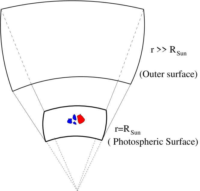
Figure 1.: Schematic illustration of the volume in which the photospheric-to-coronal portions of a bipolar active region are imbedded. It is assumed that at the outer surface, the magnetic field is negligibly small, and that the side-wall boundaries are sufficiently far away from the active region that they do not contribute to the Gauss’ theorem surface integral. Note that at the photosphere, the outward surface normal vector ${\mathbf{\hat{n}}}$ points in the $-{\mathbf{\hat{r}}}$ direction. The red and blue colors represent the upward and downward vertical fluxes in the active region. figure:spherevolume

If we assume that the upper surface of the volume is sufficiently far above the active region that the magnetic field integrated over that surface is negligible, and that the side walls are also sufficiently distant that there is negligible magnetic field contribution from those integrals as well, then the only surface that will contribute will be the photosphere near the active region, where the magnetic fields are strong. In that case, ${\mathbf{\hat{n}}}=-{\mathbf{\hat{r}}}$, and ${\mathbf{B}}\cdot{\mathbf{\hat{n}}}=-B_{r}$, where $B_{r}$ is the radial field component. The surface integral then results in the following two equations for the upward ($i.e.$ radial) and horizontal components of the Lorentz force [$F_{r}$] and [${\mathbf{F}}_{h}$]:

$$F_{r}={1\over 8\pi}\int_{A_{\mathrm{ph}}}\mathrm{d}A\,(B_{h}^{2}-B_{r}^{2})\ ,\ilabel{equation:forceup}$$ (5)

and

$${\mathbf{F}}_{h}=-{1\over 4\pi}\int_{A_{\mathrm{ph}}}\mathrm{d}A\,B_{r}{\mathbf{B}}_{h}\ .\ilabel{equation:forcesideways}$$ (6)

Here, ${\mathbf{B}}_{h}$ represents the components of ${\mathbf{B}}$ in the directions parallel to the photosphere, which we will henceforth refer to as the “horizontal” directions. The quantity $B_{h}^{2}={\mathbf{B}}_{h}\cdot{\mathbf{B}}_{h}$, and $A_{\mathrm{ph}}$ is the area of the photospheric domain containing the active region. If the active region is sufficiently small in spatial extent and magnetically isolated from other strong magnetic fields, one can approximate this surface integral as an integral over $x$ and $y$ in Cartesian coordinates, with the upward direction represented as $z$ instead of $r$.

The restrictions given above regarding the side-wall contributions to the Gauss’s law integrals can be relaxed if the volume of the domain is extended to a global volume: an integral over the entire outer atmosphere of the Sun. In this case, there are no side-wall boundaries to worry about, and $A_{\mathrm{ph}}$ coincides with the entire photospheric surface of the Sun. The outer spherical surface boundary is assumed to be sufficiently far from the Sun that it makes no significant contribution to the Gauss’s law surface integral. Thus, integrals over the entire solar surface of Equations (equation:forceup) and (equation:forcesideways) should represent the total Lorentz force acting on the Sun’s outer atmosphere. If one sets the total Lorentz force to zero, the above surface integrals yield well-known constraint equations on force-free fields (Low1985), with the Cartesian version of the equations being used to test the force-free condition of photospheric and chromospheric vector magnetograms (Metcalf1995). If the magnetic-field distribution is not force-free, but the atmosphere is observed to be static, then presumably the Lorentz forces are balanced by other forces such as gas-pressure gradients and gravity.

Wang2010 have found from an analysis of eleven large (X-class) flaring active regions that the vector magnetic field is always observed to change after a flare in the sense that the magnetic field becomes “more horizontal” than before the flare. The change is observed to occur on a timescale of a few minutes, and in some cases on a time scale as fast as the sample spacing (one minute) permits. What are the implications of this observational result on the Lorentz force acting on the solar atmosphere?

To address this question, we first take the temporal derivative of Equations (equation:forceup) and (equation:forcesideways) to find

$${\partial F_{r}\over\partial t}={1\over 8\pi}\int_{A_{\mathrm{ph}}}\mathrm{d}A\,{\partial\over\partial t}(B_{h}^{2}-B_{r}^{2})\ ,\ilabel{equation:dforceupdt}$$ (7)

and

$${\partial{\mathbf{F}}_{h}\over\partial t}=-{1\over 4\pi}\int_{A_{\mathrm{ph}}}\mathrm{d}A\,{\partial\over\partial t}(B_{r}{\mathbf{B}}_{h})\ .\ilabel{equation:dforcesidewaysdt}$$ (8)

Next, we assume the fields are observed to change over a time duration $\delta t$, and integrate the temporal derivatives of the Lorentz-force contributions to find the changes to the Lorentz-force components $\delta F_{r}$ and $\delta{\mathbf{F}}_{h}$:

$$\delta F_{r}={1\over 8\pi}\int_{A_{\mathrm{ph}}}\mathrm{d}A\,(\delta B_{h}^{2}-\delta B_{r}^{2})\ ,\ilabel{equation:deltafr}$$ (9)

and

$$\delta{\mathbf{F}}_{h}=-{1\over 4\pi}\int_{A_{\mathrm{ph}}}\mathrm{d}A\,\delta(B_{r}{\mathbf{B}}_{h})\ ,\ilabel{equation:deltafh}$$ (10)

where at a fixed location in the photosphere

$$\delta B_{h}^{2} \equiv \int_{0}^{\delta t}\mathrm{d}t\,{\partial\over\partial t}B_{h}^{2}=B_{h}^{2}(\delta t)-B_{h}^{2}(0)\ ,$$ (11)

$$\delta B_{r}^{2} \equiv \int_{0}^{\delta t}\mathrm{d}t\,{\partial\over\partial t}B_{r}^{2}=B_{r}^{2}(\delta t)-B_{r}^{2}(0)\ ,$$ (12)

$$\delta(B_{r}{\mathbf{B}}_{h}) \equiv \int_{0}^{\delta t}\mathrm{d}t\,{\partial\over\partial t}(B_{r}{\mathbf{B}}_{h})=B_{r}(\delta t){\mathbf{B}}_{h}(\delta t)-B_{r}(0){\mathbf{B}}_{h}(0)\ .$$ (13)

These quantities are simply the observed changes in the magnetic variables that occur over the course of a flare. Note that if the flaring active region is near disk center, so that the observed transverse magnetic field is a good approximation to the horizontal field, then the expression for $\delta F_{r}$ can be evaluated without having to perform the 180^∘ disambiguation of the vector magnetogram data – only the amplitude of the horizontal field enters into the expression.

If the change in the Lorentz force is significant only within small areas of the photosphere, then the only contribution to the global-area integral will be from the smaller domains where the changes are significant, potentially simplifying the evaluation of Equations (equation:deltafr) and (equation:deltafh).

We now argue that in the outer atmosphere of flaring active regions, the impulse from the changed Lorentz force dominates all other forces. First, from energetic considerations, the magnetic field is believed to be the source of energy for eruptive flares and coronal mass ejections: Forbes2000 and Hudson2007 have argued that no other known source of energy can provide the observed kinetic energy of outward motion observed in coronal mass ejections, and there simply is no other viable source for the thermal and radiated energy known to be released in solar flares. Second, apart from the Lorentz force, the only other significant forces known to be operating on the solar atmosphere are gas-pressure gradients and gravity. To evaluate the change in the gas-pressure gradient forces in the outer atmosphere, one can perform a Gaussian volume integral over the outer solar atmosphere of the vertical component of the gas-pressure gradient force. The net change in the vertical force is just the difference between the gas pressure change at the top of the Gaussian volume from that at the bottom. If the plasma $\beta$ in the solar atmosphere is low, as is generally the case in active regions, it seems unlikely that this will be as significant as the change of the Lorentz force. Nevertheless, in Section section:otherforce, we will consider perturbations to the gas pressure at the photosphere and discuss their effectiveness. In the case of the gravitational force, unless the plasma has moved a huge distance ($\approx R_{\odot}$) away from the Sun on the time-scale of the observed field change, the gravitational force acting on the given mass of the plasma within the Gaussian volume must be approximately the same, and hence the change in the gravitational force should be small.

The results of Wang2010, in which the field is observed to become more horizontal after the occurrence of eruptive flares, is thus consistent with an upward impulse acting on the outer atmosphere, so we identify this impulse as the photospheric magnetic-field signature of the force driving a magnetic eruption. To estimate the magnitude of the impulse, we make the simple assumption that the change in the Lorentz force in Equations (equation:deltafr) and (equation:deltafh) occurs linearly with time from $t=0$ to $t=\delta t$. We denote the mass of the plasma that is eventually ejected as $M_{\mathrm{ejecta}}$, and we assume the fluid velocity averaged over this plasma is zero prior to the eruption. The Lorentz impulse will then be related to the ejecta’s momentum by

$${1\over 2}\,\delta F_{r}\,\delta t=M_{\mathrm{ejecta}}v_{r}\ilabel{equation:impulser}$$ (14)

and

$${1\over 2}\,\delta{\mathbf{F}}_{h}\,\delta t=M_{\mathrm{ejecta}}{\mathbf{v}}_{h}\ ,\ilabel{equation:impulseh}$$ (15)

where $v_{r}$ is the upward (radial) component of the velocity of the ejecta after the impulse, and ${\mathbf{v}}_{h}$ is the resulting horizontal component of the ejecta velocity. Note that if $v_{r}$ is less than the escape velocity [$v_{\mathrm{e}}\equiv(2GM_{\odot}/R_{\odot})^{1/2}$], the ejecta will ultimately be stopped by gravity and will not result in an eruption. If $v_{r}$ exceeds $v_{e}$, we assume that the ejecta can become a coronal mass ejection (CME). This means that for a given observation of magnetic-field changes in a flaring active region, there is an upper limit to the mass of any resulting CME given by

$$M_{\mathrm{CME}}<{1\over 2}\,{\delta F_{r}\,\delta t\over v_{\mathrm{e}}}\ .\ilabel{equation:massul}$$ (16)

For the magnetic-field changes in the 2 November 2003 flare studied by Hudson2008, they estimate a change in the Lorentz-force surface density of $2500$ ${\rm dyne\ cm}^{-2}$, and with the estimated area over which the change occurs, a total force of $\approx 10^{22}\ {\rm dyne}$. This is probably an underestimate for the total upward force, since this case was taken from the study by Sudol2005, in which only the line-of-sight contributions were measured. A more extensive analysis of a larger dataset of flares (Petrie2010) has since shown several other cases of comparable or even larger Lorentz forces for some X-class flares. Assuming a time scale of ten minutes for the photospheric magnetic fields to change (from the temporal evolution results of Sudol2005 and Petrie2010) then results in an upper limit on the mass of any CME coming from this flaring active region of $4.9\times 10^{16}\ {\rm g}$.

Having an expression for the Lorentz-driven impulse in the horizontal directions (Equation (equation:impulseh)) could be useful in determining the initial deflection of the ejecta away from a radial trajectory. The initial trajectory direction can be determined by examining the ratio of the horizontal components of $\delta{\mathbf{F}}_{h}$ to $\delta F_{r}$.

What effect do these Lorentz force changes, and the impulses driven by them, have on the response of the solar interior plasma at and below the photosphere? To estimate the change in the Lorentz force acting on the solar interior (the interior is defined here to be the plasma that extends from the photosphere downward), one can perform almost exactly the same Gaussian volume exercise as above, but using a sub-surface volume instead of an outer atmosphere volume. By performing the global integral of the Lorentz-force density over the entire volume below the photosphere, one can see that both the absolute Lorentz forces (Equations (equation:forceup) and (equation:forcesideways)) and the changes in the Lorentz forces (equations (equation:deltafr) and (equation:deltafh)) involve exactly the same photospheric surface terms as for the outer solar atmosphere, except that the outward surface normal ${\mathbf{\hat{n}}}$ is in the $+{\mathbf{\hat{r}}}$ direction instead of in the $-{\mathbf{\hat{r}}}$ direction. Thus the three components of the Lorentz force, and the flare-induced changes in the Lorentz force, have exactly the same magnitude, but opposite sign from the Lorentz forces acting on the solar atmosphere – the Lorentz force changes acting on the interior and the solar atmosphere are exactly balanced:

$$\delta F_{r,\mathrm{interior}}={1\over 8\pi}\int_{A_{\mathrm{ph}}}\mathrm{d}A\,(\delta B_{r}^{2}-\delta B_{h}^{2})\ ,\ilabel{equation:deltafrdown}$$ (17)

and

$$\delta{\mathbf{F}}_{h,\mathrm{interior}}={1\over 4\pi}\int_{A_{\mathrm{ph}}}\mathrm{d}A\,\delta(B_{r}{\mathbf{B}}_{h})\ .\ilabel{equation:deltafhdown}$$ (18)

The radial component of the force change acting on the solar interior was identified as a magnetic jerk by Hudson2008.

To relate these results (Equations equation:deltafrdown – equation:deltafhdown) to those of Hudson2008, we note that if we let $z$ be in the upward direction, and use $x$ and $y$ to denote the horizontal directions, and further make the first order approximation that $\delta B_{h}^{2}\approx 2B_{x}\delta B_{x}+2B_{y}\delta B_{y}$, and that $\delta B_{z}^{2}\approx 2B_{z}\delta B_{z}$, where $\delta B_{x},\ \delta B_{y},\ \delta B_{z}$ are the observed changes in $B_{x}$, $B_{y}$, and $B_{z}$, then Equation (equation:deltafrdown) yields the un-numbered expression given by Hudson2008, assumed to be integrated over the vector-magnetogram area:

$$\delta F_{z,\mathrm{interior}}\approx{1\over 4\pi}\int\,\mathrm{d}A\,(-B_{x}\ \delta B_{x}-B_{y}\delta B_{y}+B_{z}\delta B_{z})\ .\ilabel{equation:hfw}$$ (19)

If Equation (equation:hfw) is evaluated over the flaring active region, such that surface terms on the vertical side walls make no significant contributions to the Gaussian integral, and the amplitude of the field-component changes is small compared to their initial values, then this expression should be robust and accurate. For future investigations of vector-magnetogram data, we believe that Equations (equation:deltafrdown) – (equation:deltafhdown) will generally be more useful than Equation (equation:hfw) since they do not assume the first-order appoximation, and the horizontal components of the force are included.

Since we assert that the Lorentz-force change is the dominant force acting in the outer solar atmosphere, and that this force drives an eruptive impulse, it follows from conservation of momentum that an equal and opposite impulse must be applied on the plasma in the solar interior, and that at least initially, the force driving this impulse is the Lorentz force identified in Equations (equation:deltafrdown) and (equation:deltafhdown). However, we expect that once the impulse has penetrated more than a few pressure scale heights into the solar interior, that the disturbance will propagate mainly as a gasdynamic-pressure disturbance (acoustic wave), since the plasma $\beta$ is thought to increase very rapidly with depth below the photosphere. For a more general discussion about momentum balance issues in solar flares, see Hudson2011, included in this topical issue.

Putting all of this together, we suggest that there is an observationally testable relationship between the measured Lorentz-force change and the outward momentum of the erupting ejecta that occurs over the course of an eruptive flare, and that the Lorentz force responsible for the eruption should also drive a downward-moving impulse into the solar interior. The downward-moving impulse could potentially be the source of observed “sunquake” acoustic emission detected with helioseismic techniques (Kosovichev1998; Moradi2007; Kosovichev2011) for some solar flares. Thus we suggest the possibility of using helioseismology to study eruptive solar flares, if the detailed wave mechanics of the impulse moving downward into the interior can be better characterized and better understood.

3 Other Disturbances in the Force

section:otherforce

We argue above that assuming that the plasma $\beta$ in the flaring active region is small implies that changes to gas-pressure gradients during a flare are most likely unimportant compared to changes in the Lorentz force. Nevertheless, the flare-induced gas-pressure change from energy deposited in the flare atmosphere has been considered in the past to be a viable candidate for the agent that excites flare-associated helioseismic disturbances (Kosovichev1995). Another suggested mechanism is heating near the solar photosphere driven by radiative backwarming of strong flaring emission occurring higher up in the solar atmosphere (Donea2006; Lindsey2008; Moradi2007). We consider each of these possibilities in the following sections.

3.1 Pressure Changes Driven by Flare Gasdynamic Processes

section:gasbag

During the impulsive phase of flares, emission in the hard X-ray and $\gamma$-ray energy range is typically emitted from small, rapidly moving kernels in the chromosphere of the flaring active region ($e.g.$ Fletcher2007). This emission is generally assumed to be the signature of energy release in the form of a large flux of energetic electrons. Energetic electrons in the 10 – 100 KeV range that impinge on the solar atmosphere will emit nonthermal bremsstrahlung radiation from Coulomb collisions with the ambient ions in the atmosphere, and will also rapidly lose energy via Coulomb collisions with ambient electrons, resulting in strong atmospheric heating (Brown1971). This results, in turn, in a large gas pressure increase in the upper chromosphere, due to rapid chromospheric evaporation. Kosovichev1995 proposed that this large pressure increase is the agent responsible for flare-driven helioseismic waves into the solar interior that have been observed.

Can this pressure increase in the flare chromosphere result in a sufficiently great pressure change at the photosphere to be significant compared to the observed changes in the Lorentz force? To investigate this question, we show that any gasdynamic disturbance that reaches the photosphere will propagate first as a shock-like disturbance (a “chromospheric condensation”) followed by the propagation of a weaker disturbance that can be treated in the acoustic limit ($v/c_{s}\ll 1$), and we then describe the work necessary to determine whether this acoustic disturbance has a perturbed pressure that can be comparable in strength to the Lorentz-force disturbance we considered in Section section:maxwell. The first task is to estimate the pressure increase in the flare chromosphere that drives the chromospheric condensation.

The pressure increase in the flare chromosphere occurs when plasma that was originally at chromospheric densities is heated to coronal temperatures. The size of the pressure increase depends on the details of how the heating is applied to the pre-flare atmosphere. If the flux of non-thermal electrons is increased very suddenly, and with a sufficiently great amplitude to exceed the maximum ability of the upper chromosphere to radiate away the non-thermal electron energy flux, this results in “explosive evaporation” (Fisher1985a, Fisher1985b). In this case, the location of the flare transition region moves very quickly to a significantly greater depth in the atmosphere. The column depth of this location can be determined by applying the suggestion of Lin1976, equating the non-thermal electron heating rate with the maximum radiative cooling rate, assuming a transition region temperature. The validity of this approach was subsequently verified in the numerical simulations of Fisher1985a. The plasma between the original and flare transition region column depths then explodes, driving violent mass motion both upwards and downwards.

Fisher1987 developed an analytical model for the explosive evaporation process, including estimates for the maximum pressure achieved during explosive evaporation, in terms of the portion of the total non-thermal electron energy flux, $F_{\mathrm{evap}}$, that is deposited between the original and flare transition-region column depths. In Figure figure:fratioplot, we explore explosive evaporation by first showing the computed ratio of $F_{\mathrm{evap}}$ to the total flux of non-thermal electrons $F_{\mathrm{nte}}$ for many possible cases of explosive evaporation, assuming a range of preflare atmospheric coronal pressure, values of the assumed low-energy cutoff [$E_{c}$], the electron spectral index [$\delta$] (see Section III of Fisher1985a for definitions of $E_{c}$ and $\delta$), and the total flux of non-thermal electrons $F_{\mathrm{nte}}$. Preflare coronal pressures include a low value of $0.3\ \mathrm{dyne\ cm}^{-2}$ (diamonds), corresponding to a tenuous pre-flare coronal density, and a higher value of $3.0\ \mathrm{dyne\ cm}^{-2}$ (triangles), corresponding to a denser pre-flare corona. Values of $E_{c}$ include $10\ \mathrm{KeV}$ (blue), $20\ \mathrm{KeV}$ (green), and $25\ \mathrm{KeV}$ (red). Electron spectral index [$\delta$] values include 4 (solid curves), 5 (dotted curves), and 6 (dashed curves). Rather than assuming a sharp low-energy cutoff to the spectrum, which produces an unphysical cusp in the non-thermal-electron heating rate as a function of column depth, we adopt the modified form of the heating rate suggested in Figure 1 and Equations (9) – (11) of Fisher1985a, in which the heating rate varies smoothly with column depth. This implies the low-energy cutoff [$E_{c}$] corresponds more to a spectral rollover than a true cutoff; the detailed electron spectra corresponding to this particular rollover behavior is given in Equations (46) – (50) of Tamres1986. Once the values for $F_{\mathrm{evap}}$ have been obtained, one can find the average per-particle heating rate in the explosively evaporating region and use Equations (38) – (39) from Fisher1987 to compute the maximum pressure due to explosive evaporation. The resulting values are shown as the colored triangles and diamonds in Figure figure:pmaxplot as functions of the flux of energy driving explosive evaporation.

We also compute the maximum pressure using an entirely different assumption for how chromospheric evaporation occurs. If the energy flux of non-thermal electrons increases more slowly than the time scale for which explosive evaporation occurs, or if the non-thermal electron energy is simply dumped into the corona and transition region through bulk heating, then chromospheric evaporation will still occur, and the pressure will still increase, but not as violently as assumed in the model of Fisher1987. In the Appendix of Fisher1989a, it was shown by considering the dynamics of chromospheric evaporation driven via thermal conduction that the maximum pressure is given approximately by Equation (32) of Fisher1989a. We use this expression to compute a second estimate for the maximum pressure driven by chromospheric evaporation, using the energy flux deposited above the flare transition region from the assumed atmospheric and electron spectral characteristics described earlier. The results are shown as the black diamonds and triangles in Figure figure:pmaxplot.

Note that both sets of estimates for the maximum pressure result in the scaling $P_{\mathrm{max}}\sim F_{\mathrm{evap}}^{2/3}\rho_{\mathrm{co}}^{1/3}$, where $\rho_{\mathrm{co}}$ is the preflare coronal mass density. This result is consistent with what one might find from a simple dimensional analysis; the only difference between the two estimates is simply a different constant of proportionality that results from the detailed assumptions in the two different evaporation models.

In addition to these estimates described above, we also plot in Figure figure:pmaxplot the maximum pressure as a function of the estimated energy flux driving evaporation achieved in the two largest-flux simulations of Fisher1985a, two cases from Abbett1999, and the highest-flux case from Allred2005. Note that in all cases, the results from the gasdynamic simulations are either close to the approximated maximum pressures from the estimates derived above, or else are bracketed by our estimates. This is even true when the assumptions used in deriving the approximate results are not strictly adhered to in the simulations. We therefore can feel some confidence that our simpler estimates will probably bracket most cases. In particular, the explosive evaporation estimates (colored triangles and diamonds) seem to provide good upper limits to the maximum pressure due to chromospheric evaporation found from any of the simulations. By examining Figures figure:fratioplot and figure:pmaxplot, we conclude that for large flare non-thermal electron energy fluxes $\approx 10^{11}{\rm\ erg\ s}^{-1}{\rm\ cm}^{-2}$, the maximum pressure increase in the chromosphere is $\approx 2000\ {\rm\ dyne\ cm}^{-2}$, and in most cases, considerably less than this. In summary, to achieve gas-pressure increases this high requires the highest non-thermal energy fluxes and a very rapid onset of these high energy fluxes.

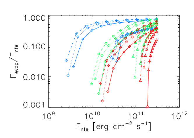
Figure 2.: Fraction of the total non-thermal electron energy flux [$F_{\mathrm{nte}}$] that goes into driving explosive chromospheric evaporation as a function of $F_{\mathrm{nte}}$. Diamonds indicate a pre-flare coronal pressure of 0.3 ${\rm dyne}\ {\rm cm}^{-2}$, while triangles indicate a higher pre-flare coronal pressure of 3.0 ${\rm dyne}\ {\rm cm}^{-2}$. Blue symbols indicate a 10 KeV low-energy cutoff, green indicates a 20 KeV low-energy cutoff, and red indicates a 25 KeV low-energy cutoff. Solid curves indicate an electron spectral index $\delta=4$, dotted curves $\delta=5$, and dashed curves $\delta=6$. figure:fratioplot

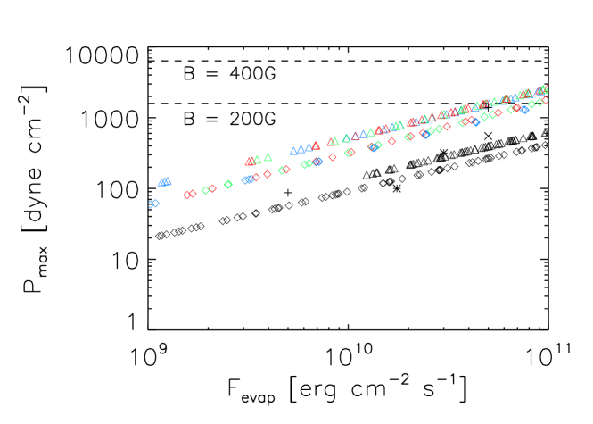
Figure 3.: Maximum gas pressure driven by impulsive-phase flare heating from non-thermal electrons as a function of the energy flux driving chromospheric evaporation. The colored diamonds show the maximum pressure computed using the analytical explosive evaporation model of Fisher (1987), for a pre-flare coronal pressure of 0.3 ${\rm dyne}\ {\rm cm}^{-2}$, while the triangles show the the maximum pressure for a pre-flare coronal pressure of 3.0 ${\rm dyne}\ {\rm cm}^{-2}$. Blue symbols indicate a 10 KeV low-energy cutoff, green indicates a 20 KeV low-energy cutoff, and red indicates a 25 KeV low-energy cutoff. The black symbols indicate the maximum pressure using the alternative model that the non-thermal energy drives evaporation indirectly via thermal conduction from Equation (32) of Fisher (1989). The black diamonds and triangles indicate the same preflare coronal pressures as above. Note both approximations show that $P_{\mathrm{max}}\approx F_{\mathrm{evap}}^{2/3}\rho_{\mathrm{co}}^{1/3}$, where $\rho_{\mathrm{co}}$ is the preflare coronal mass density, but with different proportionality constants. Also plotted are the maximum pressures from several radiation-hydrodynamic flare simulations: The two highest flux cases in Fisher, Canfield, and McClymont (1985a,b,c) (*), two cases from Abbett and Hawley (1999) (+), and a case from Allred et al. (2005) ($\times$). The two dashed horizontal lines denote the magnetic pressure for field strengths of 200 G and 400 G, respectively.

figure:pmaxplot

The pressure increase drives not only the rapid upward motion of the evaporating plasma into the corona, but also slower, denser flows of plasma downward into the chromosphere ($e.g.$ Fisher1985c) described as “chromospheric condensations”. These dense, downward-moving plugs of plasma form behind a downward-moving shock-like disturbance driven by the pressure increase from chromospheric evaporation in flares. Simple, analytic models of the dynamic evolution of chromospheric condensations were developed by Fisher1989a. The models were found to do a good job of describing the results of more detailed numerical gasdynamic simulations. One interesting property of the models is that, during the time period that the downflow evolution is well-described in terms of chromospheric condensations, the dynamical evolution is insensitive to the details of cooling behind the downward moving front of the chromospheric condensation. Further, examination of several simulation results indicate that the gas pressure in the chromospheric condensation just behind the front of the condensation is relatively constant in time, as the condensation propagates deeper into the atmosphere. This result was used in the analytical models of the condensation dynamics (Fisher1989a). Radiative cooling immediately behind the downward moving shock at the head of the chromospheric condensation leads to densities in the condensation that are much greater than the density ahead of it. Fisher1989a showed by applying mass- and momentum-conservation jump conditions, plus differing assumptions about how the plasma is cooled, that the velocity evolution is very insensitive to the details of how the plasma is cooled, provided that the resulting density jump is large (see the comparisons in Figure 1 of that article, for example). These models predict the maximum column depth that the chromospheric condensation can penetrate into the solar atmosphere as a shock-like disturbance, in terms of the flare-induced pressure [$P_{\mathrm{max}}$] driven by electron-beam heating of the solar atmosphere. The maximum column depth of propagation [$N_{\mathrm{max}}$] is given approximately by

$$N_{\mathrm{max}}={P_{\mathrm{max}}\over\bar{m}g}\ ,\ilabel{equation:nmax}$$ (20)

where $\bar{m}\approx 1.4m_{p}$ is the mean mass per proton in the solar atmosphere, and $g=2.74\times 10^{4}{\rm\ cm\ s}^{-2}$ is the value of surface gravity. The values of $P_{\mathrm{max}}$ mentioned above result in values of $N_{\mathrm{max}}$ that are no larger than $\approx 3\times 10^{22}\ {\rm\ cm}^{-2}$. The column depth of the solar photosphere, on the other hand is $\approx 10^{24}{\rm\ cm}^{-2}$. Thus, using the chromospheric-condensation model, flare-driven pressure disturbances can propagate to at most 3% of the column depth of the photosphere as chromospheric condensations; but this does not mean that the downflows cease at this depth: it means only that the equation of motion for chromospheric condensation (Equation (10) from Fisher1989a) no longer applies when the driving pressure approaches the ambient pressure ahead of the condensation. At the depths where this occurs, downflow velocities become significantly less than the sound speed, and are therefore better treated in the acoustic limit.

Because the chromospheric-condensation model’s assumptions begin to break down at the last stages of its evolution, we then consider the subsequent downward propagation of flare-driven pressure disturbances between column depths of $\approx 3\times 10^{22}\ {\rm\ cm}^{-2}$ and $\approx 10^{24}{\rm\ cm}^{-2}$ using an entirely different approach: We assume that the disturbance can be represented by an acoustic wave, driven by a simple downward pulse corresponding to the last stages of the chromospheric condensation’s evolution. For simplicity, we assume simple, adiabatic wave evolution in an isothermal, gravitationally stratified approximation of the lower chromosphere, assuming an ideal gas equation of state, without dissipation. As described in more detail below, there are reasons to question these assumptions, but this solution allows us to demonstrate some general properties of the resulting wave evolution.

Assuming that the pre-flare chromosphere can be represented by an isothermal, gravitationally stratified atmosphere at temperature $T_{\mathrm{ch}}$ with pressure scale height $\Lambda_{P}=c_{s}^{2}/(\gamma g)$, where $c_{s}$ is the adiabatic sound speed, and $\gamma$ is the ratio of specific heats, the equation for the perturbed vertical velocity is found to be

$${\partial^{2}v\over\partial t^{2}}-c_{s}^{2}({1\over\Lambda_{P}}{\partial v\over\partial s}+{\partial^{2}v\over\partial s^{2}})=0\ .\ilabel{equation:acoustic}$$ (21)

Here, $s$ measures vertical distance in the downward direction, measured from the final position of the chromospheric condensation. We assume that at the depth where the chromospheric-condensation solution breaks down, the result of its final propagation is a downward displacement [$\Delta s$] occurring over a short time. We then want to follow this displacement, using the above acoustic-wave equation, as it propagates downward. At $s=0$, we therefore assume the temporal evolution of the velocity [$v$] is given by

$$v(s=0,t)=\Delta s\delta(t)\ ,\ilabel{equation:initialwave}$$ (22)

where $\delta(t)$ is the Dirac $\delta$-function. By performing a Laplace transform of Equation (equation:acoustic) with this assumed time behavior at $s=0$, we find

$$v(s,t)=\Delta s\ {\rm exp}\left(-{s\over 2\Lambda_{P}}\right)$$

$$\times\left[\delta(t-{s\over c_{s}})-{s\over 2\Lambda_{P}\sqrt{t^{2}-{s^{2}\over c_{s}^{2}}}}J_{1}\left(\omega_{a}\sqrt{t^{2}-{s^{2}\over c_{s}^{2}}}\ \right)H(t-{s\over c_{s}})\right]\ ,$$ (23)

where $J_{1}$ is a Bessel function, $H$ is the Heaviside function, and $\omega_{a}$ is the acoustic cutoff frequency [$\omega_{a}=c_{s}/(2\Lambda_{P})$].

Note that the solution corresponds to the downward propagation of the pulse, along with a trailing wake that oscillates at a frequency that asymptotically approaches the acoustic-cutoff frequency. While it is clear that the velocity amplitude decreases rapidly (there is an overall envelope function going as $\exp(-s/(2\Lambda_{P}))$ as the pulse propagates deeper), one can show that the perturbed pressure amplitude associated with the pulse actually increases as $\exp(s/(2\Lambda_{P}))$ as the pulse propagates deeper. It is therefore possible that the pressure amplitude of the acoustic wave could be even larger than the initial pressure [$P_{\mathrm{max}}$] of the flare chromosphere, derived above.

On the other hand, there are a number of dissipation mechanisms that our wave solution does not include, which could dramatically reduce the perturbed pressure of the resulting acoustic wave. To the extent that energy balance between radiative cooling and flare heating by the most energetic electrons is important at these depths, Fisher1985c showed in Section IV of that article that high-frequency acoustic waves were very strongly damped by radiative cooling; low-frequency acoustic waves were damped more weakly, but still attenuated on length scales of $\approx 200$ km.

To summarize, we have shown how one can estimate the peak gasdynamic pressure driven by chromospheric evaporation, and that the largest possible values of this pressure require both high energy fluxes and rapid onset of those fluxes to produce explosive evaporation. We have also shown that the ensuing shock- like disturbance (a chromospheric condensation) can only propagate down to roughly 3% of the column depth of the photosphere, but that the dying chromospheric condensation can continue propagating downward as an acoustic wave to photospheric depths. We found a wave solution that is dispersive, consisting of both a pulse and a trailing wake, and used a simplified example to show that the perturbed pressure of the acoustic wave can increase as the wave propagates down towards the photosphere. We then discuss a number of wave-dissipation mechanisms that may efficiently extract energy from the wave. The extent to which the gas-dynamic-excited acoustic wave at the photosphere is important relative to the Lorentz-force perturbation (Section section:maxwell) will depend critically on a detailed evaluation of these wave-dissipation effects on the acoustic solution, and it is beyond the scope of what we can present here.

3.2 Pressure Changes Driven by Radiative Backwarming

section:backwarming

Observations of the spatial and temporal variation of optical continuum (white light) emission and hard X-ray emission during solar flares show an intimate temporal, spatial, and energetic relationship between the presence of energetic electrons in the flare chromosphere and white-light emission from the solar photosphere (Hudson1992; Metcalf2003; Chen2005; Watanabe2010). One possible component mechanism of this connection is radiative backwarming of the continuum-emitting layers by UV and EUV line and free–bound emission that is excited by energetic electrons penetrating into the flare chromosphere, at some distance above the photosphere. Since the radiative cooling time of the flare chromosphere immediately below the regions undergoing chromospheric evaporation is so short (Fisher1985c), the temporal variation of UV and EUV line emission from plasma within the $10^{4}-10^{5}\mathrm{K}$ temperature range will closely track heating by energetic electrons, detected as hard X-ray emission emitted from footpoints in the flare chromosphere. The backwarming scenario is illustrated schematically in Figure figure:backwarming.

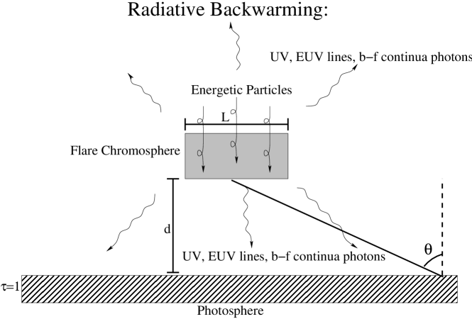
Figure 4.: Schematic illustration of radiative backwarming in a solar flare. Energetic electrons are stopped collisionally in the upper flare chromosphere, raising the temperature of the plasma there. The increased energy input is balanced by an increased radiative output in the form of EUV and UV line radiation, and the emission of free–bound continua from H and other ions. This radiation is emitted in all directions, but a signficant fraction of it is re-absorbed in optically thick layers near the solar photosphere. These layers respond with an increase of temperature and pressure, with an amplitude that will depend sensitively on the energy flux, area coverage, and timing of the impinging radiation. The emitting layer is assumed to be at a height $d$ above the photosphere. The shape of the emitting layer seen from directly below is assumed to be a circular, with diameter $L$. At an arbitrary location on the photospheric surface, the angle between the direction to the center of the source and the vertical direction is $\theta$, and the corresponding direction cosine $\mu=\cos(\theta)$. figure:backwarming

Estimates of the continuum opacity and atmospheric density near the solar photosphere indicate that the layer responsible for most of the optical continuum emission is about one continuum photon mean-free path thick, or roughly 70 km. Thus most of the energy from the impinging backwarming radiation will be reprocessed into optical continuum emission within a thin layer near the solar photosphere.

Does the absorption of this radiation within this thin layer result in a significant downward force, via a pressure perturbation from enhanced heating? This mechanism has been suggested by Donea2006, Moradi2007, and Lindsey2008 as a potential source for “sunquake” acoustic emission seen during a few solar flares. Here, we compare and contrast this mechanism of creating a force perturbation with that from the Lorentz force change described earlier.

The simplest estimate of the pressure change is to assume that the backheated photospheric plasma is frozen in place during the heating process, and that its temperature will rise to a level where the black-body radiated energy flux equals the combined output of the preflare solar radiative flux plus the incoming flare energy flux due to backwarming.

What is the flux of energy from backwarming available to heat the photosphere? In order to compute this flux, we must first estimate the fraction of the non-thermal electron energy flux that is balanced by chromospheric UV/EUV line and free–bound continuum emission, and the fraction of this radiated energy that impinges on the nearby solar photosphere. We can use the estimate presented in Section section:gasbag and plotted in Figure figure:fratioplot for $F_{\mathrm{evap}}/F_{\mathrm{nte}}$ to find the flux of energy $F_{\mathrm{rad}}$ that is converted from non-thermal electrons into radiated energy,

$$F_{\mathrm{rad}}\simeq(1-F_{\mathrm{evap}}/F_{\mathrm{nte}})\ F_{\mathrm{nte}}\ .\ilabel{equation:frad}$$ (24)

Not all of this energy flux will be available for backwarming, because the resulting radiation is emitted isotropically, while the photosphere lies beneath the radiating source. If the lateral dimension $L$ of the illuminating region is much larger than the distance $d$ above the photosphere, then up to half the radiated energy flux will irradiate the photosphere directly beneath the source (see Figure figure:backwarming). If the ratio $d/L$ is of order unity, on the other hand, there is a substantially reduced geometrical dilution factor [$f_{\mathrm{geom}}$] that must multiply $F_{\mathrm{rad}}$ to determine the flux of radiated energy that is incident on the photosphere beneath the source. We estimate the geometrical dilution factor $f_{\mathrm{geom}}$ as

$$f_{\mathrm{geom}}={1\over 2}\left(1-{2d/L\over\sqrt{1+4(d/L)^{2}}}\right)\mu^{3}\ ,$$ (25)

where for simplicity this expression assumes that the shape of the irradiating source shown in Figure figure:backwarming is a circular disk of diameter $L$. If the position of interest on the photosphere is not directly beneath the illuminating source, but instead is located at an angle $\theta$ away from the vertical direction (see Figure figure:backwarming), this expression includes a factor of $\mu^{3}$, where $\mu=\cos(\theta)$, accounting for both increased distance from the source to the given point on the photosphere and the oblique angle of the irradiating source relative to the normal direction. With the geometrical dilution factor determined, this results in the following estimate of the elevated photospheric temperature [$T$]:

$$\sigma T^{4}=\sigma T_{0}^{4}+f_{\mathrm{geom}}F_{\mathrm{rad}}\ ,\ilabel{equation:tblackbody}$$ (26)

where $T_{0}$ is the non-flare photospheric effective temperature. This expression can be re-written as

$${\Delta T\over T_{0}}=\left(1+{f_{\mathrm{geom}}F_{\mathrm{rad}}\over\sigma T_{0}^{4}}\right)^{1/4}-1\ ,\ilabel{equation:deltatovert}$$ (27)

where $\Delta T/T_{0}$ is the ratio of the temperature rise to the preflare photospheric temperature.

Figure 5.: Computed ratio of geometrical dilution factor to the plane-parallel value of $1/2$ as a function of $d/L$, where $d$ is the height of the source above the photosphere, and $L$ is the diameter of the source, which is assumed to have a circular shape. The asterisk on the curve shows the value for $d/L=1.4$ (see text). The plot assumes $\mu=1$, $i.e.$ for a point on the photosphere directly beneath the irradiating source. figure:geomplot

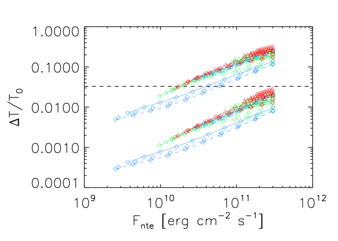
Figure 6.: Computed ratio of temperature rise to background photospheric temperature as a function of the flux of energy in non-thermal electrons, using Equation (equation:deltatovert). Diamonds indicate a pre-flare coronal pressure of 0.3 ${\rm dyne}\ {\rm cm}^{-2}$, while triangles indicate a higher pre-flare coronal pressure of 3.0 ${\rm dyne}\ {\rm cm}^{-2}$. Blue symbols indicate a 10 KeV low-energy cutoff, green indicates a 20 KeV low-energy cutoff, and red indicates a 25 KeV low-energy cutoff. Solid curves indicate an electron spectral index $\delta=4$, dotted curves $\delta=5$, and dashed curves $\delta=6$. The geometrical dilution factor in the upper set of curves was set to $1/2$, consistent with plane-parallel geometry, in which the horizontal dimension $L$ of the illuminating region is much greater than the height $d$ of the illuminating region above the photosphere. The lower set of curves was computed by setting $d/L$ to $1.4$, consistent with a 1000 km diameter source illuminating the photosphere from a height of 1400 km (see text). The dashed horizontal line indicates the temperature ratio needed to match a vertical Lorentz force surface density of $2500\ \mathrm{dyne\ cm}^{-2}$. figure:tratio

Next, we estimate the height above the photosphere for the source of the backwarming radiation. To do this we find the change in depth between the preflare and flare transition region, using the same explosive evaporation model described in Section section:gasbag. For cases where the assumed flux in non-thermal electrons exceeds $10^{11}$ $\mathrm{erg\ cm}^{-2}\mathrm{\ s}^{-1}$, the depth of the flare transition region relative to the preflare transition region moves downwards by distances ranging from $\approx$ 100 km for the dense preflare corona, up to $\approx$ 600 km for the tenuous preflare corona. The primary source of the backwarming radiation will be in the layers immediately below the flare transition region. Assuming an approximate distance between the photosphere and preflare transition region of 2000 km ($e.g.$ model F of Vernazza1981), thus leads to an expected distance that ranges from 1400 to 1900 km between the backwarming source and the photosphere. We then estimate the geometrical dilution of a UV/EUV emitting flare kernel with roughly $L\approx 1000\ \mathrm{km}$ in horizontal extent (based on estimated flare kernel areas of roughly one arcsecond²) located in the flare chromosphere at a distance $d=1400\ \mathrm{km}$ above the photosphere, in keeping with the above distance estimates, and find a geometrical dilution factor assuming $d/L=1.4$ of $f_{\mathrm{geom}}=0.029$, shown as the asterisk in Figure figure:geomplot. The low value of $f_{\mathrm{geom}}$ stems from the fact that the source as seen from the photosphere subtends a solid angle of less than 0.4 steradians, compared with the $4\pi$ steradians over which the radiation is emitted.

In Figure figure:tratio, we use Equation (equation:deltatovert) to plot the temperature enhancement as a function of non-thermal electron energy flux for two different assumed values of $f_{\mathrm{geom}}$, $1/2$, corresponding to a widespread (plane-parallel) source of backwarming radiation, and $0.029$, corresponding to $d/L=1.4$. This Figure shows a wide range in possible values of $\Delta T/T$ for a commonly assumed range of non-thermal electron energy fluxes. This fact, coupled with the wide range of possible values for $f_{\mathrm{geom}}$, illustrates the difficulty in making broad conclusions about the effectiveness of backwarming in perturbing the photosphere.

The horizontal line in Figure figure:tratio corresponds to the temperature ratio that would lead to a pressure increase comparable to the estimated Lorentz force surface density of $2500\ \mathrm{dyne\ cm^{-2}}$ for the large flare discussed in Hudson2008. Here, we adopt a pre-flare photospheric pressure of $7.6\times 10^{4}\ {\rm\ dyne\ cm}^{-2}$ (see model S of Dalsgaard1996). In the limit of large-scale source size ($d\ll L$), $f_{\mathrm{geom}}=1/2$, and there is a wide range of non-thermal electron energy fluxes which yield pressure increases which could be comparable or even greater than the above Lorentz force example. On the other hand, for a small 1000 km flare kernel size, we find temperature enhancements that are comparable to the candidate Lorentz force value only for the very largest non-thermal electron energy fluxes we have considered. Regarding the non-thermal electron energy flux levels, we must point out that recent RHESSI and Hinode observations (Krucker2011) of the white-light flare of 6 December 2006 indicate a value of $F_{\mathrm{nte}}$ of $10^{12}-10^{13}\ \mathrm{erg\ cm}^{-2}\mathrm{\ s}^{-1}$, a value that greatly exceeds our assumed energy flux range in Figure figure:tratio, and which would result in a pressure increase that greatly exceeds the Lorentz force estimate in that figure, even for a small value of $L/d$. We also point out, on the other hand, an observed sunquake (15 February 2011), for which no white-light enhancement was observed at all (C.A. Lindsey and J.C. Martínez-Oliveras, 2011, Private communication), indicating that in this case backwarming did not play a signficant role.

We must caution that our perturbed pressure estimates for backwarming are probably overestimates. Our treatment assumes the temperature changes instantaneously (ignoring the time-lag due to the finite heat capacity of the photospheric plasma), and it assumes the photospheric plasma is frozen in place and does not respond dynamically to the increased heating (the plasma should expand in response to the enhanced heating on a sound-crossing time – for a 70 km thick photospheric layer, with $C_{s}\approx 8{\rm\ km\ s}^{-1}$, this is $\approx$ ten seconds). This treatment also ignores the possibility of multi-step radiative reprocessing, in which the backwarming radiation that reaches the photosphere comes not from the primary source in the flare chromosphere, but from secondary backheating sources, where the UV line emission is first converted via backwarming to other radiation mechanisms ($e.g.$ H bound–free continuum emission), before finally reaching the photosphere. Each step of a multi-step reprocessing will result in further dilution of the energy flux reaching the photosphere.

In summary, our simple estimate of backwarming-induced temperature and pressure increases shows a wide range of possible outcomes. To be competitive with the Lorentz-force surface density taken from Hudson2008, requires either backwarming sources that are much wider than their height above the photosphere, or for small flare kernel sizes, energy fluxes well in excess of $10^{11}\ \mathrm{erg\ cm^{-2}\ s^{-1}}$. Our pressure enhancement estimates are probably upper limits, since they ignore heat capacity effects, expansion of the heated photospheric plasma, and any secondary reprocessing. Nevertheless these estimates provide useful guidelines for future, more detailed investigations of flare-driven backwarming.

4 Conclusions

section:conclusions

We derive an expression for the vertical and horizontal components of the Lorentz-force change implied by observed magnetic-field changes occurring over the course of a solar flare. The Lorentz-force change acting on the outer solar atmosphere, Equations (equation:deltafr) – (equation:deltafh), is balanced exactly by a corresponding Lorentz force change acting on the photosphere and below: Equations (equation:deltafrdown) – (equation:deltafhdown). The Lorentz force change, integrated over the time period over which the change occurs, defines an impulse. The impulse defines a momentum increase, given in Equations (equation:impulser) and (equation:impulseh). The radial component of the impulse, acting on the outer solar atmosphere, is then used to derive an upper limit to the mass of CME ejecta that escape from the Sun: Equation (equation:massul).

We show that our expression for the vertical Lorentz-force change acting on the solar interior, Equation (equation:deltafrdown), generalizes our earlier result in Hudson2008, in that it includes horizontal as well as vertical (radial) forces. It is also more accurate, in that it does not assume a first-order expansion of changes in the magnetic field.

The balance between the Lorentz forces acting on the solar atmosphere and the solar interior leads us to suggest a possible connection between the upward momentum in flare ejecta and the downward momentum in the solar interior, and leads to the possibility of using helioseismic measurements of “sunquakes” to study the properties of eruptive flares and CMEs.

For the purpose of further elucidating the physical origins of “sunquake” acoustic emission, we also estimate force perturbations in the photosphere due to changes in gas pressure driven by chromospheric evaporation and from radiative backwarming of the photosphere during solar flares. We find, for chromospheric evaporation in flares, an upper limit of $\approx 2000\ {\rm\ dyne\ cm}^{-2}$ for a pressure increase in the upper chromosphere. We show that this pressure increase will lead to the downward propagation of a chromospheric condensation, (a dense region behind a downward moving shock-like disturbance), but the chromospheric condensation can propagate to column depths of at most a few percent of the photospheric depth; the subsequent propagation to the photosphere is by means of an acoustic disturbance. Whether this acoustic disturbance is significant at photospheric depths, when compared to the Lorentz force per unit area, is not yet clear, and will require a more detailed analysis of acoustic-wave propagation and dissipation effects in the solar chromosphere. We compare the Lorentz force to gas-pressure changes driven by radiative backwarming, and find the latter mechanism could be comparable to, or greater than, the Lorentz force if the region being energized by flare non-thermal electron heating has a horizontal extent much greater than its height above the photosphere, or for smaller heated regions, if the nonthermal electron energy flux greatly exceeds $10^{11}\ \mathrm{erg\ cm^{-2}\ s^{-1}}$. We caution that our estimates of pressure changes due to backheating are probably overestimates.

To summarize, the primary source for energy release in eruptive solar flares is most likely the solar magnetic field in strong-field, low-$\beta$ active regions. It then makes sense that changes in the magnetic field itself will have a more direct and larger impact on the atmosphere than changes that are due to secondary flare processes, such as the production of energetic particles, gasdynamic motions, and enhanced radiative output, all of which are assumed to be driven ultimately by the release of magnetic energy.

Acknowledgements

This work was supported by the NASA Heliophysics Theory Program (grants NASA-NNX08AI56G and NASA-NNX11AJ65G), by the NASA LWS TR&T program (grants NNX08AQ30G and NNX11AQ56G), by the NSF SHINE program (grants ATM0551084 and ATM-0752597), by the NSF core AGS program (grant ATM-0641303) funding our efforts in support of the University of Michigan’s CCHM project, NSF NSWP grant AGS-1024682, and NSF core grant AGS-1048318. HSH acknowledges support from NASA Contract NAS5-98033. We thank the US taxpayers for making this research possible. We wish to acknowledge the role that Dick Canfield has played in realizing the importance of global momentum balance in the dynamics of solar-flare plasmas, through several seminal papers on this topic in the 1980s and 1990s. We thank the referee, Charlie Lindsey, for noting an error in our initial discussion of the depth dependence of the gas pressure perturbation for downward propagating acoustic waves. We also thank him for providing an exceptionally thoughtful, thorough, and detailed critique of this article, which improved it greatly.

References

- Abbett and Hawley (1999) Abbett, W.P., Hawley, S.L.: 1999, Dynamic Models of Optical Emission in Impulsive Solar Flares. ApJ 521, 906 – 919. doi:10.1086/307576.
- Allred et al. (2005) Allred, J.C., Hawley, S.L., Abbett, W.P., Carlsson, M.: 2005, Radiative Hydrodynamic Models of the Optical and Ultraviolet Emission from Solar Flares. ApJ 630, 573 – 586. doi:10.1086/431751.
- Brown (1971) Brown, J.C.: 1971, The Deduction of Energy Spectra of Non-Thermal Electrons in Flares from the Observed Dynamic Spectra of Hard X-Ray Bursts. Sol. Phys. 18, 489 – 502. doi:10.1007/BF00149070.
- Chen and Ding (2005) Chen, Q.R., Ding, M.D.: 2005, On the Relationship between the Continuum Enhancement and Hard X-Ray Emission in a White-Light Flare. ApJ 618, 537 – 542. doi:10.1086/425856.
- Christensen-Dalsgaard et al. (1996) Christensen-Dalsgaard, J., Dappen, W., Ajukov, S.V., Anderson, E.R., Antia, H.M., Basu, S., Baturin, V.A., Berthomieu, G., Chaboyer, B., Chitre, S.M., Cox, A.N., Demarque, P., Donatowicz, J., Dziembowski, W.A., Gabriel, M., Gough, D.O., Guenther, D.B., Guzik, J.A., Harvey, J.W., Hill, F., Houdek, G., Iglesias, C.A., Kosovichev, A.G., Leibacher, J.W., Morel, P., Proffitt, C.R., Provost, J., Reiter, J., Rhodes, E.J. Jr., Rogers, F.J., Roxburgh, I.W., Thompson, M.J., Ulrich, R.K.: 1996, The Current State of Solar Modeling. Science 272, 1286 – 1292. doi:10.1126/science.272.5266.1286.
- Donea et al. (2006) Donea, A., Besliu-Ionescu, D., Cally, P.S., Lindsey, C., Zharkova, V.V.: 2006, Seismic Emission from A M9.5-Class Solar Flare. Sol. Phys. 239, 113 – 135. doi:10.1007/s11207-006-0108-3.
- Fisher (1987) Fisher, G.H.: 1987, Explosive evaporation in solar flares. ApJ 317, 502 – 513. doi:10.1086/165294.
- Fisher (1989) Fisher, G.H.: 1989, Dynamics of flare-driven chromospheric condensations. ApJ 346, 1019 – 1029. doi:10.1086/168084.
- Fisher, Canfield, and McClymont (1985a) Fisher, G.H., Canfield, R.C., McClymont, A.N.: 1985a, Flare Loop Radiative Hydrodynamics - Part Seven - Dynamics of the Thick Target Heated Chromosphere. ApJ 289, 434 – 441. doi:10.1086/162903.
- Fisher, Canfield, and McClymont (1985b) Fisher, G.H., Canfield, R.C., McClymont, A.N.: 1985b, Flare Loop Radiative Hydrodynamics - Part Six - Chromospheric Evaporation due to Heating by Nonthermal Electrons. ApJ 289, 425 – 433. doi:10.1086/162902.
- Fisher, Canfield, and McClymont (1985c) Fisher, G.H., Canfield, R.C., McClymont, A.N.: 1985c, Flare loop radiative hydrodynamics. V - Response to thick-target heating. ApJ 289, 414 – 424. doi:10.1086/162901.
- Fletcher et al. (2007) Fletcher, L., Hannah, I.G., Hudson, H.S., Metcalf, T.R.: 2007, A TRACE White Light and RHESSI Hard X-Ray Study of Flare Energetics. ApJ 656, 1187 – 1196. doi:10.1086/510446.
- Forbes (2000) Forbes, T.G.: 2000, A review on the genesis of coronal mass ejections. J. Geophys. Res. 105, 23153 – 23166.
- Hudson (2007) Hudson, H.S.: 2007, Chromospheric Flares. In: Heinzel, P., Dorotovič, I., Rutten, R.J. (eds.) The Physics of Chromospheric Plasmas, CS-368, Astron. Soc. Pacific, San Francisco 365.
- Hudson, Fisher, and Welsch (2008) Hudson, H.S., Fisher, G.H., Welsch, B.T.: 2008, Flare Energy and Magnetic Field Variations. In: Howe, R., Komm, R.W., Balasubramaniam, K.S., Petrie, G.J.D. (eds.) Subsurface and Atmospheric Influences on Solar Activity, CS-383, Astron. Soc. Pacific, San Francisco 221 – 226.
- Hudson et al. (1992) Hudson, H.S., Acton, L.W., Hirayama, T., Uchida, Y.: 1992, White-light flares observed by YOHKOH. PASJ 44, L77 – L81.
- Hudson et al. (2011) Hudson, H.S., Fletcher, L., Fisher, G.H., Abbett, W.P., Russell, A.: 2011, Momentum Distribution in Solar Flare Processes. Sol. Phys., 340. doi:10.1007/s11207-011-9836-0.
- Kosovichev (2011) Kosovichev, A.G.: 2011, Helioseismic Response to the X2.2 Solar Flare of 2011 February 15. ApJ 734, L15 – L20. doi:10.1088/2041-8205/734/1/L15.
- Kosovichev and Zharkova (1995) Kosovichev, A.G., Zharkova, V.V.: 1995, Seismic Response to Solar Flares: Theoretical Predictions. In: Hoeksema, J.T., Domingo, V., Fleck, B., Battrick, B. (eds.) Helioseismology, SP-376, ESA, Noordwijk, 341 – 344.
- Kosovichev and Zharkova (1998) Kosovichev, A.G., Zharkova, V.V.: 1998, X-ray flare sparks quake inside Sun. Nature 393, 317 – 318. doi:10.1038/30629.
- Krucker et al. (2011) Krucker, S., Hudson, H.S., Jeffrey, N.L.S., Battaglia, M., Kontar, E.P., Benz, A.O., Csillaghy, A., Lin, R.P.: 2011, High-resolution Imaging of Solar Flare Ribbons and Its Implication on the Thick-target Beam Model. ApJ 739, 96. doi:10.1088/0004-637X/739/2/96.
- Lin and Hudson (1976) Lin, R.P., Hudson, H.S.: 1976, Non-thermal processes in large solar flares. Sol. Phys. 50, 153 – 178. doi:10.1007/BF00206199.
- Lindsey and Donea (2008) Lindsey, C., Donea, A.: 2008, Mechanics of Seismic Emission from Solar Flares. Sol. Phys. 251, 627 – 639. doi:10.1007/s11207-008-9140-9.
- Low (1985) Low, B.C.: 1985, Modeling solar magnetic structures. In: Hagyard, M. J. (ed.) Measurements of Solar Vector Magnetic Fields, NASA, Huntsville, 49 – 65.
- Metcalf et al. (1995) Metcalf, T.R., Jiao, L., McClymont, A.N., Canfield, R.C., Uitenbroek, H.: 1995, Is the solar chromospheric magnetic field force-free? ApJ 439, 474 – 481.
- Metcalf et al. (2003) Metcalf, T.R., Alexander, D., Hudson, H.S., Longcope, D.W.: 2003, TRACE and Yohkoh Observations of a White-Light Flare. ApJ 595, 483 – 492. doi:10.1086/377217.
- Moradi et al. (2007) Moradi, H., Donea, A.C., Lindsey, C., Besliu-Ionescu, D., Cally, P.S.: 2007, Helioseismic analysis of the solar flare-induced sunquake of 2005 January 15. MNRAS 374, 1155 – 1163. doi:10.1111/j.1365-2966.2006.11234.x.
- Petrie and Sudol (2010) Petrie, G.J.D., Sudol, J.J.: 2010, Abrupt Longitudinal Magnetic Field Changes in Flaring Active Regions. ApJ 724, 1218 – 1237. doi:10.1088/0004-637X/724/2/1218.
- Sudol and Harvey (2005) Sudol, J.J., Harvey, J.W.: 2005, Longitudinal Magnetic Field Changes Accompanying Solar Flares. ApJ 635, 647 – 658. doi:10.1086/497361.
- Tamres, Canfield, and McClymont (1986) Tamres, D.H., Canfield, R.C., McClymont, A.N.: 1986, Beam-induced pressure gradients in the early phase of proton-heated solar flares. ApJ 309, 409 – 420. doi:10.1086/164613.
- Vernazza, Avrett, and Loeser (1981) Vernazza, J.E., Avrett, E.H., Loeser, R.: 1981, Structure of the solar chromosphere. III - Models of the EUV brightness components of the quiet-sun. ApJS 45, 635 – 725. doi:10.1086/190731.
- Wang and Liu (2010) Wang, H., Liu, C.: 2010, Observational Evidence of Back Reaction on the Solar Surface Associated with Coronal Magnetic Restructuring in Solar Eruptions. ApJ 716, L195 – L199. doi:10.1088/2041-8205/716/2/L195.
- Watanabe et al. (2010) Watanabe, K., Krucker, S., Hudson, H., Shimizu, T., Masuda, S., Ichimoto, K.: 2010, G-band and Hard X-ray Emissions of the 2006 December 14 Flare Observed by Hinode/SOT and Rhessi. ApJ 715, 651 – 655. doi:10.1088/0004-637X/715/1/651.