Start-up flow of a viscoelastic fluid in a pipe
with fractional Maxwell’s model

Abstract

Unidirectional start-up flow of a viscoelastic fluid in a pipe with fractional Maxwell’s model is studied. The flow starting from rest is driven by a constant pressure gradient in an infinite long straight pipe. By employing the method of variable separations and Heaviside operational calculus, we obtain the exact solution, from which the flow characteristics are investigated. It is found that the start-up motion of fractional Maxwell’s fluid with parameters $\alpha$ and $\beta$, tends to be at rest as time goes to infinity, except the case of $\beta=1$. This observation, which also can be predicted from the mechanics analogue of fractional Maxwell’s model, agrees with the classical work of Friedrich and it indicates fractional Maxwell’s fluid presents solid-like behavior if $\beta\neq 1$ and fluid-like behavior if $\beta=1$. For an arbitrary viscoelastic model, a conjecture is proposed to give an intuitive way judging whether it presents fluid-like or solid-like behavior. Also oscillations may occur before the fluid tends to the asymptotic behavior stated above, which is a common phenomenon for viscoelastic fluids.

Keywords: Viscoelastic fluid; fractional Maxwell’s model; start-up flow; pipe flow; Heaviside operational calculus.

1 Introduction

‘All things are movable and in a fluid state’, which is a famous quotation from Thales of Miletos, the first philosopher of ancient Greece.

Indeed, besides the most familiar fluids such as water and gas, most materials in nature and industry, such as milk, oil, lava, etc., can be treated and investigated as fluids. However, some of them not only have the viscosity like Newtonian fluid, but also exhibit Hooke’s elasticity. They are viscoelastic materials. Different models of viscoelastic materials were obtained and studied during the past hundreds of years; for example, Maxwell’s model, constructed by a spring and a dashpot in serial, was largely investigated in the last century.

Recently, fractional Maxwell’s model, constructed by two fractional element models in serial, attracts a lot of researchers’ interests[1][2][3][4][5][15][18][19][20]. Let $\sigma$ be the shear stress and $\epsilon$ be the shear strain. The constitutive equation for fractional Maxwell’s model is given by

$$\sigma+\lambda^{\alpha}\frac{d^{\alpha}}{dt^{\alpha}}\sigma=E\lambda^{\beta}\frac{d^{\beta}}{dt^{\beta}}\epsilon,~{}~{}~{}~{}~{}0\leq\alpha\leq\beta\leq 1,$$ (1)

where $E$ the shear modulus, and $\lambda$ is the relaxation time.

In the case of $\alpha=0$, equation (1) degenerates to

$$\sigma=\frac{1}{2}E\lambda^{\beta}\frac{d^{\beta}}{dt^{\beta}}\epsilon,$$

which is just the constitutive relation of a fractional element model with the shear modulus $E/2$. In fact, the usual expression for a fractional element model was first introduced by Scott Blair[6][7]

$$\sigma=E_{s}\lambda^{\beta}\frac{d^{\beta}}{dt^{\beta}}\epsilon,$$ (2)

where $E_{s}$ is the shear modulus. The mechanics analogue of a fractional element model can be found in [1][2][8][10].

In the case of $\alpha=\beta=1$, equation (1) degenerates to the constitutive relationship of classical Maxwell’s model.

Physically, fractional Maxwell’s model can be considered as two fractional element models in serial, with orders $\gamma_{1}$ and $\gamma_{2}$ satisfying

$$\alpha=|\gamma_{1}-\gamma_{2}|,~{}~{}~{}~{}\beta=\max\{\gamma_{1},\gamma_{2}\}.$$ (3)

Fig.1 gives the mechanics analogue of fractional Maxwell’s model, where a triangle denotes a fractional element model.

Figure 1: Mechanics analogue of fractional Maxwell’s model. A triangle denotes a fractional element model.

The continuous interest of fractional Maxwell’s model is perhaps due to the special known and unknown property of this model and due to the rapid development of fractional calculus during the last fifty years. Palade et. al. in [15] derived fractional Maxwell’s model from the linearization of the objective equation and discovered the anomalous stability behavior of the rest state in three dimensions. Tan et. al. in [3][9] studied four unsteady flows of a viscoelastic fluid with generalized Maxwell’s model between two infinite parallel plates. Vieru et. al. in [18] studied flow of a generalized Oldroyd-B fluid due to a constantly accelerating plate, which includes generalized Maxwell’s model as a limiting case. Hayat et al. [5] also discussed fractional Maxwell’s model and studied three types of unidirectional flows which were induced by general periodic oscillations of a plate. Hernández-Jiménez et. al. gave some experimental results for oscillating flows with fractional Maxwell’s model [4], which encourage more studies. Yin and Zhu [1] studied the oscillating flow with fractional Maxwell’s model in an infinitely long pipe and found interesting results, for example, the resonance peaks was discovered to be different with those of ordinary Maxwell’s model.

A lot of interests and studies were also given to the unidirectional start-up pipe flows, which has a significant practical and mathematical meaning. Zhu and Lu et. al. in [14] studied characteristics of the velocity filed and the shear stress field for an ordinary Maxwell’s fluid and discovered the oscillation phenomenon. Fetecau in [17] studied the analytic solution for an ordinary Oldroyd-B fluid and several limiting cases such as ordinary Maxwell’s fluid; the velocity profiles for the steady state are the same in all types of fluid they studied. Further, Tong et. al. in [16] studied the exact solution for the fractional Oldroyd-B model in an annular pipe by using Hankel-Laplace transform. Using similar but different methods, Zhu and Yang et. al. in [13] studied the exact solution and flow characteristics for the fractional element model with parameter $\beta$, the most fundamental model in all fractional derivative models. They found oscillation phenomenon and solid-like behavior for certain $\beta$.

As far as we know, the characteristics of start-up pipe flow with fractional Maxwell’s model have not been well-studied yet. In this paper, we investigate basic characteristics of such flows through studying the exact solution. The fluid is quiescent in the beginning in an infinitely long pipe, and then it will be suddenly started by a pressure gradient which remains constant after the starting moment.

The start-up pipe flow with a dashpot model (i.e. Newtonian fluid) is classical in fluid dynamics; with ordinary Maxwell’s model the motion would be very interesting because of the occurrence of oscillations [14]; and with the fractional element model solid-like behavior was discovered [13] as we already mentioned above. One must be curious what the interesting phenomena for fractional Maxwell’s model are and whether we can summarize a way to deduce the characteristic of a certain viscoelastic model if just given the constitutive relation.

This paper is organized as follows. In section 2, we present the governing equations and initial boundary conditions, and solve this initial boundary value problem through the method of variable separation and Heaviside’s operational calculus. In section 3, we discuss the flow characteristics and give some observations. In section 4, we make the conclusion and propose a conjecture.

2 Governing equation and exact solution

We consider the start-up flow of a fractional Maxwell fluid in an infinitely long pipe with the radius $a$. In the beginning, the fluid in the pipe is at rest; then it is suddenly started by a constant pressure gradient. Take the pipe axial direction as the $z$-axis. We construct a column coordinate system $(r,\theta,z)$ and let $V(r,\theta,z,t)$ denote the flow field.

Since the flow is axisymmetric, we assume $V$ only has the axial component and does not depend on $\theta$, i.e.,

$$V=u(r,t)e_{z}.$$ (4)

The governing equations of the motion are given by the continuous equation

$$\nabla\cdot V=0,$$ (5)

as well as the momentum equation

$$\rho\frac{dV}{dt}=-\nabla p+\nabla\cdot\sigma,$$ (6)

where $\frac{d}{dt}$ is the material derivative, $\rho$ is the density of the fluid, $p$ is the pressure field and $\sigma$ is the stress tensor field.

The start-up flow considered is driven by the pressure gradient field given by

$$\frac{\partial p}{\partial z}(t)=-Gh(t),$$ (7)

where $G$ is a constant and $h(t)$ is the Heaviside function, defined by $h(t)=0,~{}t<0;~{}h(t)=1,~{}t\geq 0$.

The constitutive equation (1) gives:

$$\sigma_{rz}+\lambda^{\alpha}\frac{\partial^{\alpha}}{\partial t^{\alpha}}\sigma_{rz}=E\lambda^{\beta}\frac{\partial^{\beta-1}}{\partial t^{\beta-1}}\frac{\partial u}{\partial r}.$$ (8)

The initial and boundary conditions are given by

$$u(a,t)=0,~{}~{}u(0,t)<\infty,~{}~{}~{}u(r,0)=\frac{\partial u}{\partial t}(r,0)=0,~{}~{}~{}~{}t>0,~{}0\leq r\leq a.$$ (9)

Substituting (4) to equations (5) and (6), and considering (7) and (8), we find

$$\rho\Big{(}1+\lambda^{\alpha}\frac{\partial^{\alpha}}{\partial t^{\alpha}}\Big{)}\frac{\partial u}{\partial t}=\Big{(}1+\lambda^{\alpha}\frac{\partial^{\alpha}}{\partial t^{\alpha}}\Big{)}Gh+E\lambda^{\beta}\frac{\partial^{\beta-1}}{\partial t^{\beta-1}}\Big{(}\frac{1}{r}\frac{\partial u}{\partial r}+\frac{\partial^{2}u}{\partial r^{2}}\Big{)}.$$ (10)

Let the radius $a$ be the characteristic length, $\rho a^{2}/E\lambda$ be the characteristic time, and $Ga^{2}/E\lambda$ be the characteristic velocity. By simple algebraic manipulations, we get the dimensionless governing equation and the dimensionless initial-boundary conditions:

$$\frac{\partial u}{\partial t}+\lambda^{\alpha}\frac{\partial^{\alpha+1}}{\partial t^{\alpha+1}}u-\lambda^{\beta-1}\frac{\partial^{\beta-1}}{\partial t^{\beta-1}}\Big{(}\frac{1}{r}\frac{\partial u}{\partial r}+\frac{\partial^{2}u}{\partial r^{2}}\Big{)}=1+\lambda^{\alpha}\frac{t^{-\alpha}}{\Gamma(1-\alpha)},$$ (11)

$0\leq r<1,~{}t>0,$

and

$$u(1,t)=0,~{}~{}u(0,t)<\infty,~{}~{}~{}t>0,$$ (12a)

$$u(r,0)=\frac{\partial u}{\partial t}(r,t)=0,~{}~{}~{}0\leq r<1.$$ (12b)

We use the method of variable separation and Heaviside operational calculus solving equations (11) and (12). Let

$$u(r,t)=v(r)T(t).$$ (13)

Substituting this expression to the homogenous equation of equation (11), we obtain

$$\frac{1}{v}\Big{(}\frac{1}{r}v^{\prime}(r)+v^{\prime\prime}(r)\Big{)}=\frac{T^{\prime}(t)+\lambda^{\alpha}T^{\alpha+1}(t)}{\lambda^{\beta-1}T^{\beta-1}(t)}=-k^{2},$$ (14)

where $k$ is some appropriate constant to be determined. Solving the eigenvalue problem:

$$\frac{1}{r}v^{\prime}(r)+v^{\prime\prime}(r)+k^{2}v=0,$$ (15a)

$$v(1)=0,~{}v(0)<\infty,$$ (15b)

we obtain the discrete eigenvalues

$$k_{1}<k_{2}<k_{3}<...,$$ (16)

as well as the corresponding eigenfunctions:

$$v_{m}=J_{0}(k_{m}r),~{}~{}~{}~{}~{}m=1,2,...,$$ (17)

where $k_{m}$ is the $m_{th}$ positive root of the zeroth Bessel function.

The final solution is constructed by

$$u(r,t)=\sum_{m=1}^{\infty}A_{m}T_{m}(t)J_{0}(k_{m}r),$$ (18)

where $A_{m}$, $m=1,2,3,...,$ are constants to be determined and $T_{m}(t)$ are functions of $t$ to be determined. Substituting this expression of $u(r,t)$ to equation (11), we find

$$\sum_{m=1}^{\infty}A_{m}\big{(}T_{m}^{\prime}(t)+\lambda^{\alpha}T^{\alpha+1}(t)+k_{m}^{2}\lambda^{\beta-1}T_{m}^{\beta-1}(t)\big{)}J_{0}(k_{m}r)=h(t)+\frac{\lambda^{\alpha}t^{-\alpha}}{\Gamma(1-\alpha)};$$ (19)

since

$$h(t)+\frac{\lambda^{\alpha}t^{-\alpha}}{\Gamma(1-\alpha)}=\Big{(}h(t)+\frac{\lambda^{\alpha}t^{-\alpha}}{\Gamma(1-\alpha)}\Big{)}\sum_{m=1}^{\infty}\frac{2J_{0}(k_{m}r)}{k_{m}J_{1}(k_{m})},~{}(0<r<1),$$ (20)

comparing the coefficients of the eigenfunctions appearing in equations (19) and (20) we have

$$A_{m}=\frac{2}{k_{m}J_{1}(k_{m})},$$ (21)

as well as

$$T_{m}^{\prime}(t)+\lambda^{\alpha}T_{m}^{\alpha+1}(t)+k_{m}^{2}\lambda^{\beta-1}T_{m}^{\beta-1}(t)=h(t)+\frac{\lambda^{\alpha}t^{-\alpha}}{\Gamma(1-\alpha)}.$$ (22)

We solve equation (22) by applying Heaviside operational calculus. Let $p=\frac{d}{dt}$ and let $T_{m}(t)=Yh(t)$ where $Y$ is an operator to be determined. Noting that

$$p^{\lambda}h(t)=\frac{t^{-\alpha}}{\Gamma(1-\alpha)},$$ (23)

we have

$$Y=\frac{1+\lambda^{\alpha}p^{\alpha}}{p+\lambda^{\alpha}p^{\alpha+1}+k_{m}^{2}\lambda^{\beta-1}p^{\beta-1}}.$$ (24)

As a result,

$$T_{m}(t)=\frac{1+\lambda^{\alpha}p^{\alpha}}{p+\lambda^{\alpha}p^{\alpha+1}+k_{m}^{2}\lambda^{\beta-1}p^{\beta-1}}h(t).$$ (25)

By the definition of the Heaviside operator [11], it yields

$$T_{m}(t)=\frac{1}{2\pi\sqrt{-1}}\int_{L}\frac{1+\lambda^{\alpha}z^{\alpha}}{z^{2}+\lambda^{\alpha}z^{\alpha+2}+k_{m}^{2}\lambda^{\beta-1}z^{\beta}}e^{zt}dz.$$ (26)

where $L$ is a contour in complex $z$-plane parallel with the imaginary axis, and is determined by the requirement that there be no singularities of the integrant on the right of $L$.

The final solution we construct is given by

$$u(r,t)=\frac{1}{2\pi\sqrt{-1}}\sum_{m=1}^{\infty}\frac{2J_{0}(k_{m}r)}{k_{m}J_{1}(k_{m})}\int_{L}\frac{1+\lambda^{\alpha}z^{\alpha}}{z^{2}+\lambda^{\alpha}z^{\alpha+2}+k_{m}^{2}\lambda^{\beta-1}z^{\beta}}e^{zt}dz.$$ (27)

Substituting this equation to equation (8) and assuming the shear stress field is zero at $t=0$, we obtain

$$\sigma_{rz}=\frac{E\lambda^{\beta}}{2\pi\sqrt{-1}}\sum_{m=1}^{\infty}\frac{-2J_{1}(k_{m}r)}{J_{1}(k_{m})}\int_{L}\frac{z^{\beta-1}}{z^{2}+\lambda^{\alpha}z^{\alpha+2}+k_{m}^{2}\lambda^{\beta-1}z^{\beta}}e^{zt}dz.$$ (28)

In the case of $\alpha=0$, i.e., the case of the fractional element model, solution (27) reduces to

$$u(r,t)=\frac{1}{2\pi\sqrt{-1}}\sum_{m=1}^{\infty}\frac{2J_{0}(k_{m}r)}{k_{m}J_{1}(k_{m})}\int_{L}\frac{2}{2z^{2}+k_{m}^{2}\lambda^{\beta-1}z^{\beta}}e^{zt}dz.$$ (29)

By an inverse formula given in [10][p.p. 271-273], we can simplify expression (29):

$$u(r,t)=\sum_{m=1}^{\infty}\frac{2J_{0}(k_{m}r)}{k_{m}J_{1}(k_{m})}tE_{2-\beta,2}(-k_{m}^{2}\lambda^{\beta-1}t^{2-\beta}/2),$$ (30)

where $E_{2-\beta,2}$ is the Mittag-Leffler function. Note that the Newtonian fluid corresponds to the particular case of $(\alpha=0,~{}\beta=1)$. Substituting $\beta=1$ to equation (30), we obtain

$$u(r,t)=\sum_{m=1}^{\infty}\frac{4J_{0}(k_{m}r)}{k_{m}^{3}J_{1}(k_{m})}\big{(}1-e^{-k_{m}^{2}t/2}\big{)}=\frac{1}{2}(1-r^{2})-\sum_{m=1}^{\infty}\frac{4J_{0}(k_{m}r)}{k_{m}^{3}J_{1}(k_{m})}e^{-k_{m}^{2}t/2},$$ (31)

which is the classical dimensionless solution.

In the case of $\alpha=\beta=1$, i.e., the case of ordinary Maxwell’s model, our solution agrees with the solution obtained by Zhu et. al. [14].

3 Results and discussions

Due to the simplicity of the fractional element model, which also plays the fundamental role of constructing different fractional models, we first recall some results in [13] of start-up pipe flow for the fractional element model (Scott Blair’s model). Without lost of generality, we take $\lambda=1$ in equation (30). As Fig.2 shows, for the case

$$0<\beta<1,$$

oscillations occur just after the fluid is started; the smaller the parameter $\beta$ is, the stronger the elasticity is. And as $t$ goes to infinity, the center velocity tends to be $0$. In fact, recall the asymptotic formula for $E_{2-\beta,2}$ [10]:

$$E_{2-\beta,2}(-z)=\frac{1}{\Gamma(\beta)}\frac{1}{z}+O(z^{-2}),~{}~{}~{}~{}~{}~{}z\rightarrow+\infty,$$ (32)

We know from this formula that the series expression (30) is uniformly convergent at least for any fixed $r$. Let $t\rightarrow\infty$; we obtain that

$$\lim_{t\rightarrow\infty}u(r,t)=0,~{}~{}~{}~{}~{}~{}~{}0\leq r\leq 1.$$ (33)

The only exception is the case of $\beta=1$, i.e. the case of Newtonian fluid. No oscillations would occur and as $t$ goes to infinity, the center velocity will tend to be a steady constant $0.5$. In this classical case,

$$\lim_{t\rightarrow\infty}u(r,t)=\frac{1}{2}(1-r^{2}),~{}~{}~{}~{}0\leq r\leq 1.$$ (34)

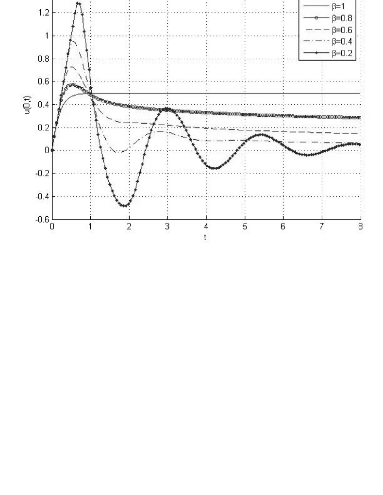
Figure 2: Center velocity with respect to $t$ for the fractional element model.

Fig. 3a) and 3b) shows the velocity profiles of different $t$, with $\beta=0.4$ and $\beta=1$ respectively, which gives intuitive pictures in mind.

$$\begin{array}[]{cc}\includegraphics[width=208.13574pt]{Fig3a_rev.eps}&\includegraphics[width=195.12767pt]{Fig3b_rev.eps}\\ \mbox{a.}~{}~{}\beta=0.4&\mbox{b.}~{}~{}\beta=1\\ \end{array}$$

Figure 3: Velocity profiles at different t for the fractional element model.

Based on these discussions of of the fractional element model, the mechanics analogue of fractional Maxwell’s model (see Fig.1) would help us do further investigates. This idea will be directly applied in the following discussions. Still we will take $\lambda=1$ without loss of generality. And we discuss the start-up flows with different $\alpha$ and $\beta$ through studying equation (27).

Fig.4 gives the curves of the center velocity with respect to $t$ when $\alpha=0.6$. It can be seen that for $0.6\leq\beta<1$, the center velocity of the pipe will tend to be $0$, which means the corresponding fractional Maxwell’s model will finally represents solid-like property; for $\beta=1$, the center velocity will tend a constant $0.25$ and the fractional Maxwell model finally represents fluid-like property. Furthermore, the smaller $\beta$ is, i.e., the stronger the elasticity of the larger order fractional element is, the stronger the oscillating phenomenon is.

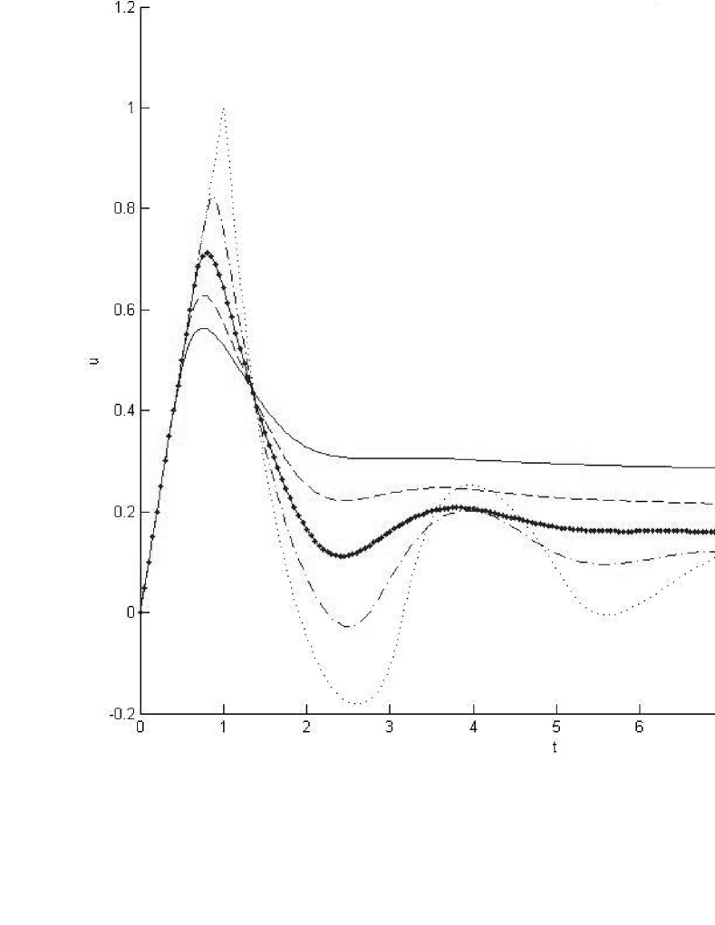
Figure 4: Center velocity with respect to $t$ for the fractional Maxwell model in the case of $\alpha=0.6$.

Fig.5 is similar with Fig.4 but the phenomenon is more clear. It gives the relation curve of center velocity with respect to $t$ with different $\alpha$, when $\beta=0.6$. It can be seen that, as $t$ goes to infinity, the center velocity of the pipe tends to be $0$, which indicates the corresponding fractional Maxwell’s model represents solid-like property. When $\alpha$ increases, i.e. the difference between the orders of the two fractional elements increases, or say the elasticity of the smaller order fractional element strengthens, the oscillating phenomenon becomes stronger, which helps the fluid to be at rest, although in short time it accelerates the fluid more.

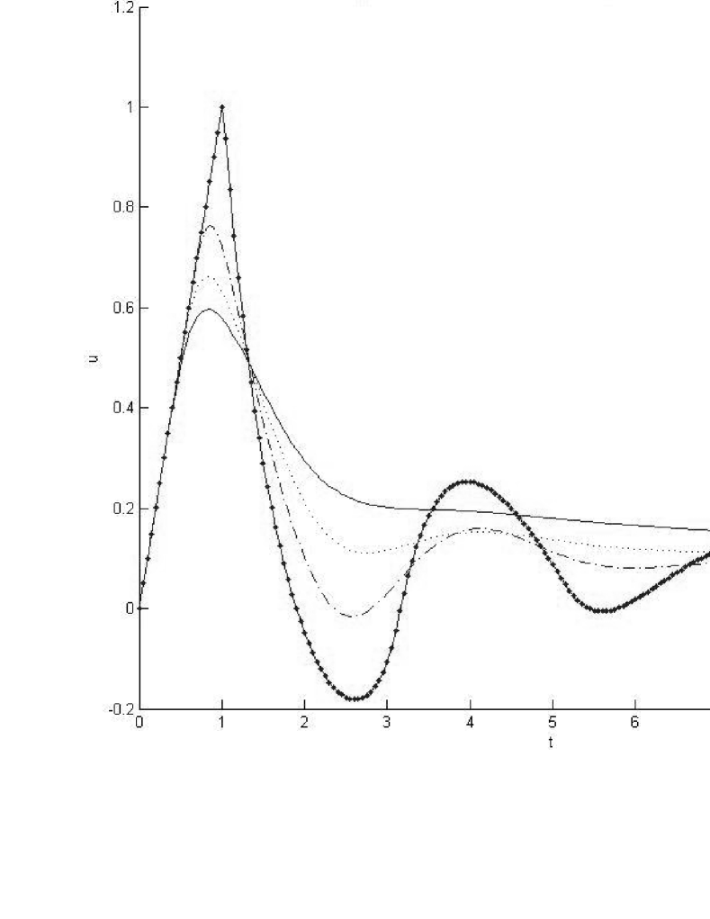
Figure 5: Center velocity with respect to $t$ for the fractional Maxwell model in the case of $\beta=0.6$.

Fig.6 shows the relation curve of the center velocity with respect to $t$ in the case of $\beta=1$. We see that if $0<\alpha\leq 1$, the center velocity will tend to a constant $0.25$ as $t$ goes to infinity; if $\alpha=0$, i.e., the case of Newtonian fluid, the center velocity will tend to $0.5$. In both cases, fractional Maxwell’s fluid will represent fluid-like property for large $t$. And when $\alpha\neq 0$, oscillation also occurs which means the fluid also has elasticity, however, since $\beta=1$, the fluid-like property will lead the way.

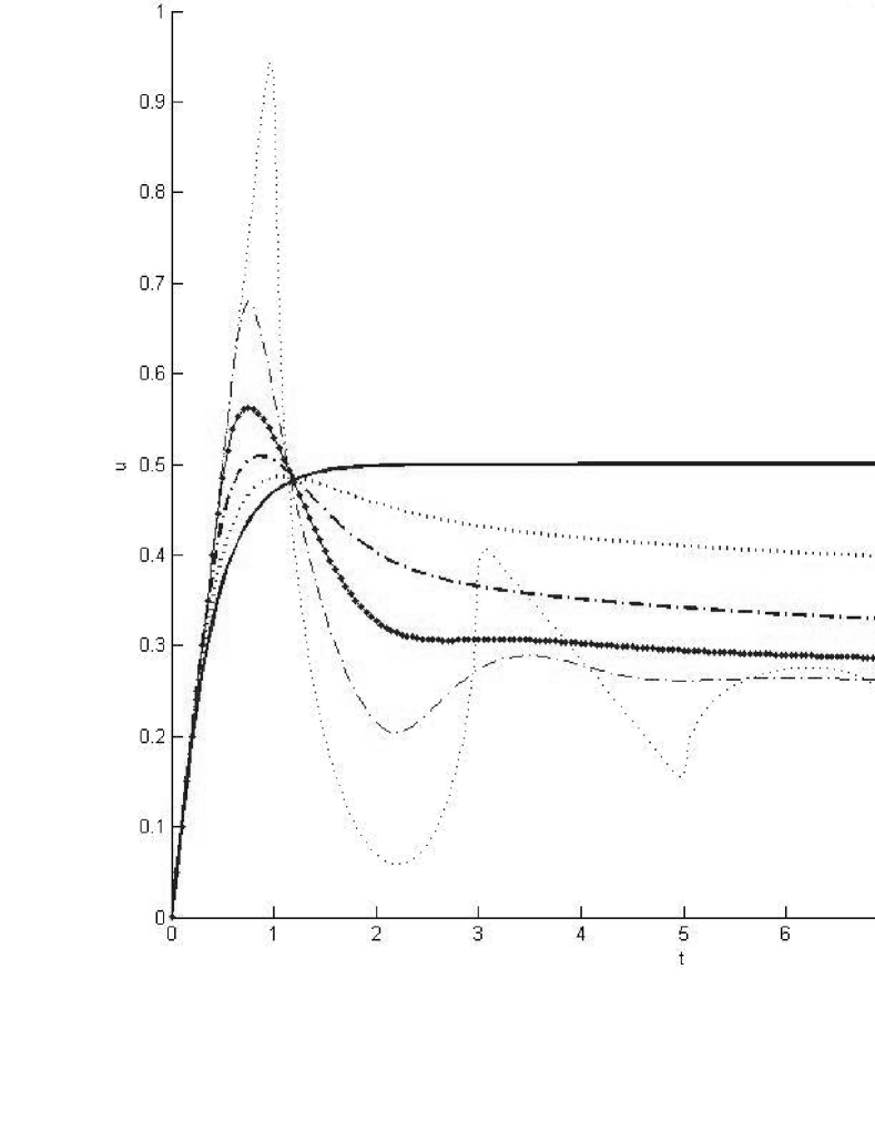
Figure 6: Center velocity with respect to $t$ for the fractional Maxwell model in the case of $\beta=1$.

It deserves to point out that these results partly agree with Friedrich’s [12], who first pointed out that the fractional Maxwell model represents solid-like property as long as $\beta<1$.

An intuitive way to deduce whether a fractional model would exhibit solid-like or fluid-like property is to consider the fractance of the mechanics analogue of the model. According to the analysis of the fractal construction of these models [10][2], we can indeed deduce solid-like property without calculations: A fractional model (which itself is not a string) presents solid-like behavior if and only if there exists a spring path from one side to the other in any spring-dashpot fractance of its mechanics analogues.

4 Conclusions

An exact solution of the start-up pipe flow with fractional Maxwell’s model is obtained and the flow characteristics are discussed.

In the case of $\beta\neq 1$, the motion of fractional Maxwell’s fluid in a pipe tends to be at rest as time goes to infinity; otherwise if $\beta=1$ the flow will have a parabolic-like profile as $t$ goes to $\infty$.

Indeed, for a Scott-Blair’s model (fractional element model) with parameter $\beta$, as long as $\beta<1$, the model presents a solid-like property. This was showed by Zhu and Yang et. al. in [13] in the study of start-up pipe flow.

For a fractional Maxwell model, i.e., two fractional element models in a serial connection, the fluid will present a solid-like property as long as the two fractional elements both present solid-like behaviors. On the other hand, if one of the fractional elements in serial is Newtonian, even the other one is a spring, the serial compound will be of fluid-like property and the flow will keep a stationary velocity profile after infinitely long time. Our result agrees with the results in [12], but from different points of views.

Moreover, the stronger the elasticity of any of the fractional element models in the serial connection is, the stronger the oscillation of the corresponding fractional Maxwell model is.

From these results for the case of fractional Maxwell’s model, we conjecture that a viscoelastic model presents a solid-like behavior if for any spring-dashpot fractance of its mechanics analogues, there exists a spring path(a path with only springs) from one side to the other. This conjecture, if proved, will generalize Friedrich’s result in [12].

Acknowledgements

We are very grateful to the referee for suggestions and constructive comments.

References

- [1] Y. Yin, K.-Q. Zhu, Oscillating flow of a viscoelastic fluid in a pipe with the fractional Maxwell model, Applied Mathematics and Computation, 173 (2006) 231-242.
- [2] K.-Q. Zhu, K.-X. Hu, D. Yang, Analysis of fractional element of viscoelastic fluids using Heaviside operational calculus, New trends in fluid mechanics research, Edited by F.-G. Zhuang and J.-C. Li, Tsinghua University Press, Springer, (2007) 506-509.
- [3] W. Tan, W. Pan, M. Xu, A note on unsteady flows of a viscoelastic fluid with the fractional Maxwell model between two parallel plates, Int. J. Non-Linear Mech. 38 (2003) 645-650.
- [4] A. Hernández-Jiménez, J. Hernández-Santiago, A. Macias-García, J. Sanchez-González, Relaxation modulus in PMMA and PTFE fitting by fractional Maxwell model, Polym. Test. 21 (2002) 325-331.
- [5] T. Hayat, S. Nadeem, S. Asghar, Periodic unidirectional flows of a viscoelastic fluid with the fractional Maxwell model, Appl. Math. Comput. 151 (2004) 153-161.
- [6] G. W. Scott Blair, The role of Psychophysics in rheology, Journal of Colloid Science, 2 (1947) 21-32.
- [7] G. W. Scott Blair, Psychoreology: link between the past and the present, Journal of Texture Studies, Vol.5 (1974) 3-12.
- [8] N. Heymans, J. C. Bauwens, Fractal rheological models and fractional differential equations for viscoelastic behavior, Rheol. Acta 33 (1994) 210-219.
- [9] W. Tan, M. Xu, Plane surface suddenly set in motion in a viscoelastic fluid with fractional Maxwell model, ACTA MECHANICA SINICA, 18 (2002).
- [10] I. Podlubny, Fractional Differential Equations, London: Academic Press, (1999).
- [11] R. Courant, D. Hilbert, Methods of mathematical physics, v.1, New York: Interscience Publishers, Inc. (1962).
- [12] C. Friedrich, Relaxation and retardation functions of the Maxwell model with fractional derivatives, Rheol. Acta 30, (1991) 151-158.
- [13] K.-Q. Zhu, D. Yang, K.-X. Hu, Fractional element of viscoelatic fluids and start-up flow in a pipe, Chinese Quaterly of Mechanics, v. 28, No. 4, (2007). (in Chinese).
- [14] K.-Q. Zhu, Y.-J. Lu, P. P. Shen, J. L. Wang, A study of start-up pipe flow of Maxwell fluid, Acta Mech. Sin., v. 35, 218, (2003). (in Chinese)
- [15] L. I. Palade, P. Attane, R. R. Huilgol, B. Mena, Anomalous stability behavior of a properly invariant constitutive equation which generalises fractional derivative models, International Journal of Engineering Sciences, 37 (1999), 315-329.
- [16] D. Tong, R. Wang, H. Yang, Exact solutions for the flow of non-Newtonian fluid with fractional derivative in an annular pipe, Science in China ser: G Physics, Mechanics and Astronomy, Vol. 48, No. 4, (2005) 485-495.
- [17] C. Fetecau, Analytical solutions for non-Newtonian fluid flows in pipe-like domains, Non-linear Mechanics 39 (2004), 225-231.
- [18] D. Vieru, Corina Fetecau, C. Fetecau, Flow of a generalized Oldroyd-B fluid due to a constantly accelerating plate, Applied Mathematics and Computation 201 (2008) 834-842.
- [19] M. Khan, S. Hyder Ali, C. Fetecau, Haitao Qi, Decay of potential vortex for a viscoelastic fluid with fractional Maxwell model, Applied Mathematical Modelling 33 (2009) 2526-2533.
- [20] D. Vieru, Corina Fetecau, M. Athar, Constantin Fetecau, Flow of a generalized Maxwell fluid induced by a constantly accelerating plate between two side walls, Z. angew. Math. Phys. 60 (2009) 334-343.