Semisimple tunnels

Abstract.

A knot in $S^{3}$ in genus-$1$ $1$-bridge position (called a $(1,1)$-position) can be described by an element of the braid group of two points in the torus. Our main results tell how to translate between a braid group element and the sequence of slope invariants of the upper and lower tunnels of the $(1,1)$-position. After using them to verify previous calculations of the slope invariants for all tunnels of $2$-bridge knots and $(1,1)$-tunnels of torus knots, we obtain characterizations of the slope sequences of tunnels of $2$-bridge knots, and of a class of tunnels we call toroidal. The main results lead to a general algorithm to calculate the slope invariants of the upper and lower tunnels from a braid description. The algorithm has been implemented as software, and we give some sample computations.

Introduction

Genus-$2$ Heegaard splittings of the exteriors of knots in $S^{3}$ have been a topic of considerable interest and recent progress. Usually these are discussed in the language of tunnels, which we will use from now on. In particular, the term tunnel will mean a tunnel of a tunnel number $1$ knot in $S^{3}$.

A rich source of examples of tunnels are the upper and lower tunnels associated to a knot positioned with bridge number $1$ with respect to a standard torus in $S^{3}$. Traditionally this is called a $(1,1)$-position of the knot, and the associated tunnels are called $(1,1)$-tunnels.

In [7], we laid out a theory of tunnels based on the disk complex of the genus-$2$ handlebody. It provides a unique construction of each knot tunnel by a sequence of “cabling” constructions, each determined by a rational “slope” invariant (the slope invariant of the first cabling is only defined in $\operatorname{{\mathbb{Q}}}/\operatorname{{\mathbb{Z}}}$). There is a second invariant, a binary sequence, which is trivial for $(1,1)$-tunnels. Thus the sequence of slope invariants is a complete invariant for a $(1,1)$-tunnel.

Naturally it is not very easy to calculate a complete invariant, but the invariants are known for all the tunnels of $2$-bridge knots [7, Section 15] and torus knots [8]. Recently, K. Ishihara [13] has given a computational algorithm which is effective for some examples.

There is a simple description of a $(1,1)$-position in terms of a braid of two points in a standard torus $T$ in $S^{3}$: Regard the braid as two arcs in $T\times I\subset S^{3}$, connect the top two points with a small trivial arc in the “upper” solid torus, and similarly for the bottom two points in the “lower” solid torus. Many different braids can give equivalent $(1,1)$-positions. Some of this ambiguity is resolved by using the quotient of the braid group by its center, which we call the reduced braid group. A braid that produces the $(1,1)$-position is called a braid description of it. In Section 1, we will examine braid descriptions and the reduced braid group, before detailing in Section 2 the first of several “maneuvers” involving braids and $(1,1)$-positions. Sections 3-6 contain a review of our general theory of tunnels, focusing on the parts needed for this paper.

Our main results are Theorems 8.1 and 9.3, which allow one to pass back and forth between a braid description of a $(1,1)$-position and the cabling slope sequence of its upper (or its lower) tunnel. This has several applications. In Example 9.4, we show how to find a braid description and use it to calculate the slope invariants for a more-or-less random example, the knot and tunnel drawn in Figure 10 of [7]. In Section 10 we use braid descriptions for the $(1,1)$-positions of all $2$-bridge knots to recover the general calculation of slope invariants obtained in [7]. We also give a precise characterization of the slope sequences that arise from tunnels of $2$-bridge knots. In Section 11, we use braid descriptions for the $(1,1)$-positions of torus knots (each has a unique $(1,1)$-position) to recover the slope invariants for their upper and lower tunnels, first found in [8].

A more theoretical application is given in Section 12, where we show that a certain property of the sequence of slope invariants corresponds to a $(1,1)$-position in $T\times I$ with no critical points in either of the $S^{1}$-directions. We call such positions toroidal positions. Among the $2$-bridge knots, only the $(2n+1,\pm 2)$-torus knots admit a toroidal position.

Our final applications make the procedure of passing between braid descriptions and slope invariants completely algorithmic. Passing from the sequence of slope invariants to a braid description is rather easy, as seen in Section 13. The other direction, detailed in Section 14, is more difficult, since anomalous infinite-slope cablings can arise (technically speaking, these are not even “cablings”) when the braid word is put into its standard form, and one must manipulate the word to eliminate these. Both of the algorithms, as well as the general slope calculations for $2$-bridge knot tunnels and $(1,1)$-tunnels of torus knots, are very effective and have been implemented in software which is available at [11] (other software there finds the invariants for the “middle” tunnels of torus knots). Sample calculations are given in Section 15.

1. Braid descriptions of $(1,1)$-positions

In this section, we recall the 2-braid group on the torus, and its quotient by its center. The latter, which we call the reduced braid group $\mathcal{B}$, or just the braid group, will play a central role in our work. We will also see how an element $\omega\in\mathcal{B}$ describes a knot $K(\omega)$, and moreover a $(1,1)$-position of that knot.

Let $T$ be a standard torus in $S^{3}$, bounding a solid torus $W\subset S^{3}$. In our figures, $W$ usually lies above $T$. Denoting the unit interval $[0,1]$ by $I$, fix a collar $T\times I\subset\overline{S^{3}-W}$ with $T=T\times\{0\}$, and denote by $V$ the solid torus $\overline{S^{3}-(W\cup T\times I)}$.

Fix a point $b\in T$, which we will refer to as the black point. Fix standard meridian and longitude curves $m$ and $\ell$ in $T$ such that

1. $m\cap\ell=b$,

2. $m$ bounds a disk in $V\cup T\times I$, and

3. $\ell$ bounds a disk in $W$.

Choose a point $w$ in $T$ that is not in $m\cup\ell$. We will refer to $w$ as the white point.

A braid can be described geometrically as a pair of disjoint arcs properly embedded in $T\times I$ such that each endpoint of the arcs is one of $b\times\{0\}$, $b\times\{1\}$, $w\times\{0\}$, or $w\times\{1\}$, and each of the arcs meets each $T\times\{s\}$ transversely in a single point. There is an obvious multiplication operation on the collection of such pairs defined by “stacking” two pairs.

Two such pairs are equivalent if there is an isotopy $J_{t}$ of $T\times I$ such that

1. $J_{0}=id_{T\times I}$,

2. $J_{t}|_{T\times\partial I}=id_{T\times\partial I}$ for $t\in[0,1]$,

3. $J_{t}(T\times\{s\})=T\times\{s\}$ for $s\in[0,1]$ and $t\in[0,1]$, and

4. $J_{1}$ sends one pair to the other pair.

The multiplication operation induces a group structure on the set of equivalence classes, producing $\mathcal{B}_{2}(T)$, the classical braid group of two points in the torus.

A presentation of $\mathcal{B}_{2}(T)$ is given in [2] and [19]. We rewrite it as

$$\langle\delta_{m},\delta_{\ell},\sigma\;|\;\delta_{m}\sigma\delta_{m}\sigma=\sigma\delta_{m}\sigma\delta_{m},\delta_{\ell}\sigma\delta_{\ell}\sigma=\sigma\delta_{\ell}\sigma\delta_{\ell},$$

$$\delta_{m}^{-1}\delta_{\ell}\delta_{m}\delta_{\ell}^{-1}=\sigma^{2},\sigma\delta_{\ell}\sigma\delta_{m}=\delta_{m}\sigma\delta_{\ell}\sigma^{-1}\rangle\ .$$

In the notation of [19], $\delta_{m}=y_{1}$, $\delta_{\ell}=x_{1}^{-1}$, and $\sigma=s_{1}$.

As seen in Figure 1, representatives of $\delta_{m}$ and $\delta_{\ell}$ slide the black point around $m$ and $\ell$ respectively, while keeping the white point fixed. A representative of $\sigma$ produces a half-twist of the two strands, as shown.

$m$ [B] at 116 285 $\ell$ [B] at 5 226

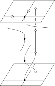
Figure 1. An imbedding representing the element $\delta_{\ell}\delta_{m}\sigma$ in $\mathcal{B}_{2}(T)$. We read braids from the top down, so in this picture, the solid torus $W$ lies above the upper copy of the torus, which is $T=T\times\{0\}$.

Now we weaken condition $(2)$ in the definition of equivalence of braids to

1. $J_{1}|_{T\times\partial I}=id_{T\times\partial I}$.

That is, we do not require that each $J_{t}$ be the identity on $T\times\partial I$ for $t\in(0,1)$. We call the new equivalence classes of the pairs of arcs under this condition reduced braids, and the group of all reduced braids is the reduced braid group denoted by $\mathcal{B}$.

The fundamental group $\pi_{1}(T)=\operatorname{{\mathbb{Z}}}\times\operatorname{{\mathbb{Z}}}$ can be regarded as a subgroup of $\mathcal{B}_{2}(T)$, as the subgroup generated by $\delta_{\ell}\sigma\delta_{\ell}\sigma$ and $\delta_{m}\sigma\delta_{m}\sigma$. Figure 2 illustrates a pair of arcs representing $\delta_{\ell}\sigma\delta_{\ell}\sigma$ in $\mathcal{B}_{2}(T)$. Using the presentation of $\mathcal{B}_{2}(T)$, one can verify that $\pi_{1}(T)$ is central in $\mathcal{B}$.

$m$ [B] at 116 176 $\ell$ [B] at 3 118

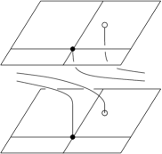
Figure 2. A braid which represent $\delta_{\ell}\sigma\delta_{\ell}\sigma$. A similar pair, winding in the $m$-direction, represents $\delta_{m}\sigma\delta_{m}\sigma$.

Weakening condition (2) to $(2^{\prime})$ has the effect of making the braids $\delta_{\ell}\sigma\delta_{\ell}\sigma$ and $\delta_{m}\sigma\delta_{m}\sigma$ trivial. On the other hand, the additional isotopies allowed by condition $(2^{\prime})$ are just products of the isotopies that move those two braids to the trivial braid (or the reverses of these isotopies). Thus $(2^{\prime})$ has the effect of adding the two relations $\delta_{m}\sigma\delta_{m}\sigma$ and $\delta_{\ell}\sigma\delta_{\ell}\sigma$ to the above presentation of $\mathcal{B}_{2}(T)$, giving the following proposition.

Proposition 1.1.

The reduced braid group $\mathcal{B}$ has the presentation

$\langle\;\delta_{m},\delta_{\ell},\sigma\;|\;(\delta_{m}\sigma)^{2}=(\delta_{\ell}\sigma)^{2}=1,\;\delta_{m}^{-1}\delta_{\ell}\delta_{m}\delta_{\ell}^{-1}=\sigma^{2}\;\rangle$.

As shown in Figure 3(b), in $\mathcal{B}$ there are other representatives of $\delta_{m}$ and $\delta_{\ell}$ that slide the white point backwards along loops parallel to $m$ and $\ell$ respectively. An isotopy that moves $b\times\{0\}$ around the loop $\ell$ changes the first representative of $\delta_{\ell}$, that moves the black point strand, to the second, that moves the white point strand in the other direction. Similarly, an isotopy that moves $b\times\{0\}$ around $m$ changes the representative of $\delta_{m}$ that moves the black strand to one that moves the white strand in the other direction. These correspond to the facts that $\sigma^{-1}\delta_{\ell}^{-1}\sigma^{-1}=\delta_{\ell}$ and similarly for $\delta_{m}$.

$m$ [B] at 115 365 $\ell$ [B] at 2 306 $m$ [B] at 340 365 $\ell$ [B] at 228 306 $\alpha_{W}$ [B] at 67 338 (a) [B] at 3 350 (b) [B] at 230 350 $\alpha_{W}$ [B] at 292 338 $M$ [B] at 162 49 $L$ [B] at 63 18 $M$ [B] at 387 49 $L$ [B] at 290 18 $\alpha_{V}$ [B] at 135 3 $\alpha_{V}$ [B] at 360 3

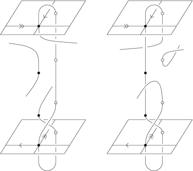
Figure 3. Two imbeddings representing the element $\delta_{\ell}\delta_{m}\sigma$ in $\mathcal{B}$. Also shown are the meridian $M$ and longitude $L$ for the reverse braid $\sigma\delta_{L}\delta_{M}$, and the trivial arcs $\alpha_{W}$ and $\alpha_{V}$ added to form the knot $K(\delta_{\ell}\delta_{m}\sigma)$. It is the trivial knot.

A nice way to understand the relations in $\mathcal{B}$ is to consider the picture of the universal cover of $T$ shown in Figure 4.

$\delta_{\ell}$ [B] at 56 149 $\delta_{\ell}$ [B] at 127 149 $\delta_{\ell}$ [B] at 56 76 $\delta_{\ell}$ [B] at 127 76 $\delta_{\ell}$ [B] at 56 4 $\delta_{\ell}$ [B] at 127 4 $\delta_{m}$ [B] at 6 125 $\delta_{m}$ [B] at 79 125 $\delta_{m}$ [B] at 152 125 $\delta_{m}$ [B] at 6 52 $\delta_{m}$ [B] at 79 52 $\delta_{m}$ [B] at 152 52 $\sigma$ [B] at 39 105 $\sigma$ [B] at 110 105 $\sigma$ [B] at 39 34 $\sigma$ [B] at 110 34

Figure 4. The universal cover of $T$, illustrating the relations in $\mathcal{B}$.

In this picture, $\delta_{\ell}$ slides the black points one unit to the right, $\delta_{m}$ slides the black points one unit downward, and $\sigma$ interchanges black and white points as indicated. The product $\sigma\delta_{\ell}\sigma$ slides the white points one unit to the right, so the effect of $\delta_{\ell}\sigma\delta_{\ell}\sigma$ is to slide both black and white one unit to the right. The relation $\delta_{m}\sigma\delta_{m}\sigma$ is similar, while the word $\delta_{m}^{-1}\delta_{\ell}\delta_{m}\delta_{\ell}^{-1}$ corresponds to a braid for which the white points are fixed and the black points travel clockwise around the squares in Figure 4, starting from the lower left-hand corner, which is the effect of $\sigma^{2}$.

Since we will have no further use for $\mathcal{B}_{2}(T)$, it is safe just to call $\mathcal{B}$ the braid group, and its elements braids.

Figure 3 also illustrates the reverse braid, which is obtained if one views the picture from below. The meridian and longitude $M$ and $L$ seen from below are analogous to the meridian $m$ and longitude $\ell$ seen from above. Note that they are interchanged, so that $\delta_{m}$ seen from below is $\delta_{L}$ and $\delta_{\ell}$ seen from below is $\delta_{M}$. Although both have the reversed orientation, a braid $\delta_{m}$ or $\delta_{\ell}$ seen from below has the point moving in reversed time, so $\delta_{m}$ becomes $\delta_{L}$ and $\delta_{\ell}$ becomes $\delta_{M}$. On the other hand, $\sigma$ seen from below still looks like $\sigma$. Thus the reverse braid has $\delta_{m}$ replaced by $\delta_{L}$ and $\delta_{\ell}$ replaced by $\delta_{M}$, with $\sigma$ unchanged, and the order of the letters reversed.

Figure 3 also illustrates the knot described by the braid $\omega$. One simply attaches the two standard arcs $\alpha_{V}$ and $\alpha_{W}$ at the bottom and top. In Figure 3, $\alpha_{V}$ and $\alpha_{W}$ are obtained from arcs $\alpha\times\{1\}$ and $\alpha\times\{0\}$ respectively, pushing the former slightly into $V$ and the latter into $W$, where $\alpha$ is a fixed arc in $T$ connecting $b$ and $w$, and meeting $m\cup\ell$ only in $b$. There are four isotopy classes of such arcs, and we select $\alpha$ to lie in the isotopy class that at $b$ leaves $m$ in the direction of the positive orientation on $\ell$ (using the orientation shown in of Figure 3) and leaves $\ell$ in the direction of the negative orienation on $m$. The lifts of $\alpha$ to the universal covering space of $T$ shown in Figure 4 leave the preimages of $b$ from the lower-left hand corner of each square.

The resulting knot $K(\omega)$ is well-defined, indeed equivalent reduced braids describe knots that are in $(1,1)$-position with respect to $T$ and are $(1,1)$-isotopic (that is, isotopic by an isotopy of $S^{3}$ preserving $T$ at all times). The notation $K(\omega)$ implicitly includes this well-defined $(1,1)$-position. We say that $K(\omega)$ is in braid position, and that the element $\omega$ is a braid description of the knot and its $(1,1)$-position (with respect to the fixed arc $\alpha$). A braid and its reverse braid describe isotopic knots, but the two $(1,1)$-positions have upper and lower tunnels interchanged.

Observe that $K(\omega)$ and $K(\omega\delta_{m})$ are $(1,1)$-isotopic, by an isotopy that pushes $K(\omega)$ across the core circle of the solid torus $V$. Similarly, $K(\omega)$ is $(1,1)$-isotopic to $K(\delta_{\ell}\omega)$, and $K(\omega)$ to both $K(\omega\sigma)$ and $K(\sigma\omega)$. In general, if $W_{0}(\delta_{\ell},\sigma)$ is a word in the letters $\delta_{\ell}$ and $\sigma$, and $W_{1}(\delta_{m},\sigma)$ is a word in $\delta_{m}$ and $\sigma$, then $K(W_{0}(\delta_{\ell},\sigma)\omega W_{1}(\delta_{m},\sigma))$ and $K(\omega)$ are $(1,1)$-isotopic. For example, the knot $K(\delta_{\ell}\delta_{m}\sigma)$ in Figure 3 is $(1,1)$-isotopic to $K(1)$, hence is trivial.

Notation 1.2.

Let $\langle\delta_{\ell},\sigma\rangle$ denote the subgroup of $\mathcal{B}$ generated by $\delta_{\ell}$ and $\sigma$, and similarly for $\langle\delta_{m},\sigma\rangle$. We will write $\omega_{1}\sim\omega_{2}$ to mean that $\omega_{1}$ and $\omega_{2}$ represent the same double coset of the form $\langle\delta_{\ell},\sigma\rangle\omega_{1}\langle\delta_{m},\sigma\rangle$, and consequently are braid descriptions of the same $(1,1)$-position.

2. Tunnels in standard position

2pt $\alpha$ [B] at 85 114 $\alpha_{W}$ [B] at 486 206 (a) [B] at 80 -2 (b) [B] at 284 -2 (c) [B] at 485 -2

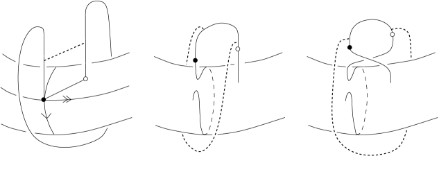
Figure 5. Introduction of an initial $\sigma^{-1}\delta_{m}^{-1}$ in order to reposition a tunnel into standard position.

In this section, we will introduce a basic maneuver. Figure 5(a) shows the torus $T=T\times\{0\}$, the portion of a $(1,1)$-knot that lies in $W$, and a tunnel arc for the “upper” (1,1)-tunnel of the knot. The segment on $T$ connecting black and white vertices is the fixed arc $\alpha$ used to define the $(1,1)$-knot from a braid description as in Section 1. The knot is not in braid position, because it does not meet $W$ in an arc parallel to $\alpha$. There is an isotopy of the knot, preserving $(1,1)$-position, that changes the placement in Figure 5(a) to the one in Figure 5(b). The arc of the knot in $W$ moves to a different arc, and a braid letter $\delta_{m}^{-1}$ appears just inside the solid torus. The tunnel arc is stretched out to wind around the core of $W$. A further $(1,1)$-isotopy changes Figure 5(b) to Figure 5(c), introducing another braid letter $\sigma^{-1}$. If we push the knot down into $T\times I$ until its intersection with $W$ is parallel to $\alpha$ (or equivalently enlarge $T\times I$ to include the portion of the knot that lies below the black and white points), then the knot is now in braid position (assuming that its original intersection with $V\cup T\times I$ is consistent with braid position).

When the upper tunnel and the portion of $K$ in $W$ consist of a tunnel arc and a trivial arc as in the portion above the black and white points in Figure 5(c), we say that $K$ and the upper tunnel (arc) are in standard position. Thus the effect of the maneuver just described is to move a tunnel arc and $K$ that appear as in Figure 5(a) so that $K$ and the tunnel are in standard position, while changing the braid represented by the portion of $K$ in $T\times I$ by premultiplication by $\sigma^{-1}\delta_{m}^{-1}$. Since $\sigma^{-1}\delta_{m}^{-1}=(\delta_{m}\sigma)^{-1}=\delta_{m}\sigma$ in $\mathcal{B}$, this is equivalent to premultiplication by $\delta_{m}\sigma$.

3. Tunnels as disks

Our previous articles [7, 8, 9, 10] give the details of our general theory of knot tunnels. Of these, [7] is the most complete, while of the shorter summaries in the other papers, the material in [8] is the closest to our present needs. For convenience of the reader, we will provide in this and the next three sections a review adapted to our work here. It also establishes notation that is used in the rest of the paper.

This section gives a brief overview of the theory in [7]. Fix a “standard” genus-2 unknotted handlebody $H$ in $S^{3}$. Regard a tunnel of $K$ as a $1$-handle attached to a neighborhood of $K$ to obtain an unknotted genus-$2$ handlebody. Moving this handlebody to $H$ by an isotopy of $S^{3}$, a cocore disk for the $1$-handle moves to a nonseparating disk in $H$. The indeterminacy due to the choice of isotopy is exactly the Goeritz group, which is the group of path components of the space of orientation-preserving homeomorphisms of $S^{3}$ that take $H$ onto $H$. Consequently, the collection of all tunnels of all tunnel number $1$ knots, up to orientation-preserving homeomorphism, corresponds to the orbits of nonseparating disks in $H$ under the action of the Goeritz group. Indeed, it is convenient for us to define a tunnel to be an orbit of nonseparating disks in $H$ under the action of the Goeritz group.

Work of Scharlemann, Akbas, and Cho [1, 6, 16] gives a very good understanding of the way that the Goeritz group acts on the disks in $H$. As detailed in [7], the orbits, i.e. the tunnels, can be arranged in a treelike structure which encodes much of the topological structure of tunnel number $1$ knots and their tunnels.

When a nonseparating disk $\tau\subset H$ is regarded as a representative of a tunnel, or simply a tunnel itself, the corresponding knot is a core circle of the solid torus that results from cutting $H$ along $\tau$. This knot is denoted by $K_{\tau}$. For example, in the handlebody shown in Figure 6, a core circle of the solid torus cut off by the middle disk is a trefoil knot.

A disk $\tau$ in $H$ is called primitive if there is a disk $\tau^{\prime}$ in $\overline{S^{3}-H}$ such that $\partial\tau$ and $\partial\tau^{\prime}$ cross in one point in $\partial H$. Equivalently, $K_{\tau}$ is the trivial knot in $S^{3}$. All primitive disks are equivalent under the action of the Goeritz group. This equivalence class is the unique tunnel of the trivial knot.

A primitive pair is an isotopy class of two disjoint nonisotopic primitive disks in $H$. A primitive triple is defined similarly. All primitive pairs are equivalent under the Goeritz group, as are all primitive triples.

It is important to understand that a triple of nonseparating disks in $H$ corresponds to an isotopy class of $\theta$-curves in $H$, specifically, the $\theta$-curve whose arcs are “dual” to the three disks— each arc cuts across exactly one of the three disks once, each disk meets exactly one of the three arcs, and each of the balls obtained by cutting $H$ along the union of the three disks deformation retracts to the portion of the $\theta$-curve that it contains. This $\theta$-curve is “unknotted” in $S^{3}$, that is, the closure of the complement of a regular neighborhood is a genus-$2$ handlebody. Thus an orbit of such triples under the Goeritz group corresponds to an isotopy class in $S^{3}$ of unknotted $\theta$-curves.

4. Slope disks and cabling arcs

This section gives the definitions needed for computing the slope invariants that will be discussed in Section 5. Fix a pair of disjoint nonseparating disks $\lambda$ and $\rho$ (for “left” and “right”) in the standard unknotted handlebody $H$ in $S^{3}$, as shown abstractly in Figure 6. The pair $\{\lambda,\rho\}$ is arbitrary, so in the true picture in $H$ in $S^{3}$, they will typically look a great deal more complicated than the pair shown in Figure 6. Let $N$ be a regular neighborhood of $\lambda\cup\rho$ and let $B$ be the closure of $H-N$. The frontier of $B$ in $H$ consists of four disks which appear vertical in Figure 6. Denote this frontier by $F$, and let $\Sigma$ be $B\cap\partial H$, a sphere with four holes.

2pt $\lambda$ [B] at -18 136 $\rho$ [B] at 595 136

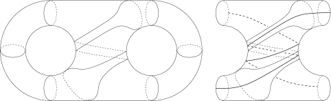
Figure 6. A slope disk of $\{\lambda,\rho\}$, and a pair of its cabling arcs contained in $B$.

A slope disk for $\{\lambda,\rho\}$ is an essential disk in $H$, possibly separating, which is contained in $B-F$ and is not isotopic to any component of $F$. Any loop in $\Sigma$ that is not homotopic into $\partial\Sigma$ is the boundary of a unique slope disk. (Throughout our work, “unique” means unique up to isotopy in an appropriate sense.) If two slope disks are isotopic in $H$, then they are isotopic in $B$. The boundary of a slope disk always separates $\Sigma$ into two pairs of pants.

An arc in $\Sigma$ whose endpoints lie in two different boundary circles of $\Sigma$ is called a cabling arc. Figure 6 shows a pair of cabling arcs disjoint from a slope disk. A slope disk is disjoint from a unique pair of cabling arcs, and each cabling arc determines a unique slope disk.

Each choice of nonseparating slope disk for a pair $\mu=\{\lambda,\rho\}$ determines a correspondence between $\operatorname{{\mathbb{Q}}}\cup\{\infty\}$ and the set of isotopy classes of slope disks of $\mu$, as follows. Fixing a nonseparating slope disk $\tau$ for $\mu$, write $(\mu;\tau)$ for the ordered pair consisting of $\mu$ and $\tau$.

Definition 4.1.

A perpendicular disk for $(\mu;\tau)$ is a disk $\tau^{\perp}$, with the following properties:

1. $\tau^{\perp}$ is a slope disk for $\mu$.

2. $\tau$ and $\tau^{\perp}$ intersect transversely in one arc.

3. $\tau^{\perp}$ separates $H$.

There are infinitely many choices for $\tau^{\perp}$, but because $H\subset S^{3}$ there is a natural way to choose a particular one, which we call $\tau^{0}$. It is illustrated in Figure 7. To construct it, start with any perpendicular disk and change it by Dehn twists of $H$ about $\tau$ until the core circles of the complementary solid tori have linking number $0$ in $S^{3}$.

2pt $\lambda^{+}$ [B] at 148 298 $\rho^{+}$ [B] at 437 300 $\lambda^{-}$ [B] at 149 -25 $\rho^{-}$ [B] at 433 -21 $\lambda$ [B] at -15 140 $\tau$ [B] at 376 141 $\rho$ [B] at 594 140 $K_{\rho}$ [B] at 210 222 $K_{\lambda}$ [B] at 369 222 $\tau^{0}$ [B] at 291 298

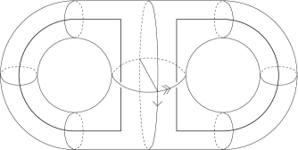
Figure 7. The slope-zero perpendicular disk $\tau^{0}$. It is chosen so that $K_{\lambda}$ and $K_{\rho}$ have linking number $0$.

For calculations, it is convenient to draw the picture as in Figure 7, and orient the boundaries of $\tau$ and $\tau^{0}$ so that the orientation of $\tau^{0}$ (the “$x$-axis”), followed by the orientation of $\tau$ (the “$y$-axis”), followed by the outward normal of $H$, is a right-hand orientation of $S^{3}$. At the other intersection point, these give the left-hand orientation. The coordinates will be unaffected by changing which of the disks in $\{\lambda,\rho\}$ is called $\lambda$ and which is $\rho$.

Let $\widetilde{\Sigma}$ be the covering space of $\Sigma$ such that:

1. $\widetilde{\Sigma}$ is the plane with an open disk of radius $1/8$ removed at each point with coordinates in $\operatorname{{\mathbb{Z}}}\times\operatorname{{\mathbb{Z}}}+(\frac{1}{2},\frac{1}{2})$.

2. The components of the preimage of $\tau$ are the vertical lines with integer $x$-coordinate.

3. The components of the preimage of $\tau^{0}$ are the horizontal lines with integer $y$-coordinate.

Figure 8 shows a picture of $\widetilde{\Sigma}$ and a fundamental domain for the action of its group of covering transformations, which is the orientation-preserving subgroup of the group generated by reflections in the half-integer lattice lines (that pass through the centers of the missing disks). Each circle of $\partial\widetilde{\Sigma}$ double covers a circle of $\partial\Sigma$.

2pt $\lambda^{+}$ [B] at 65 66 $\lambda^{-}$ [B] at 138 66 $\lambda^{+}$ [B] at 209 66 $\lambda^{-}$ [B] at 281 66 $\rho^{+}$ [B] at 65 142 $\rho^{-}$ [B] at 138 142 $\rho^{+}$ [B] at 209 142 $\rho^{-}$ [B] at 281 142 $\lambda^{+}$ [B] at 65 210 $\lambda^{-}$ [B] at 138 210 $\lambda^{+}$ [B] at 209 210 $\lambda^{-}$ [B] at 281 210 $\rho^{+}$ [B] at 65 286 $\rho^{-}$ [B] at 138 286 $\rho^{+}$ [B] at 209 286 $\rho^{-}$ [B] at 281 286 $\lambda^{+}$ [B] at 420 0 $\lambda^{-}$ [B] at 740 0 $\rho^{+}$ [B] at 420 310 $\rho^{-}$ [B] at 745 309 $\tau^{0}$ [B] at 738 158 $\tau$ [B] at 578 244

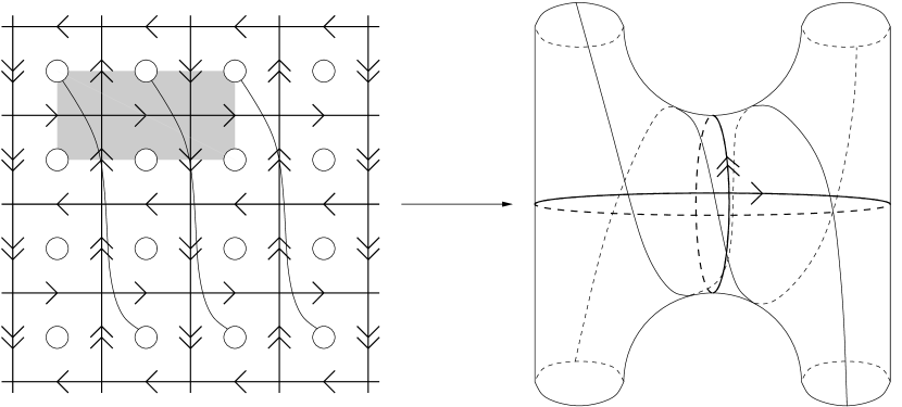
Figure 8. The covering space $\widetilde{\Sigma}\to\Sigma$, and some lifts of the pair of $[1,-3]$-cabling arcs from Figure 6. The shaded region is a fundamental domain.

Each lift of a cabling arc $\alpha$ of $\Sigma$ to $\widetilde{\Sigma}$ runs from a boundary circle of $\widetilde{\Sigma}$ to one of its translates by a vector $(p,q)$ of signed integers, defined up to multiplication by the scalar $-1$. In this way $\alpha$ receives a slope pair $[p,q]=\{(p,q),(-p,-q)\}$, and is called a $[p,q]$-cabling arc. The corresponding slope disk is assigned the slope pair $[p,q]$ as well, and can be called a $[p,q]$-slope disk. The cabling arcs in Figure 8 are $[1,-3]$-cabling arcs. A corresponding $[1,-3]$-slope disk is the one shown in Figure 6.

An important observation is that a $[p,q]$-slope disk is nonseparating in $H$ if and only if $q$ is odd. Both happen exactly when a corresponding cabling arc has one endpoint in $\lambda^{+}$ or $\lambda^{-}$ and the other in $\rho^{+}$ or $\rho^{-}$.

Definition 4.2.

Let $\lambda$, $\rho$, and $\tau$ be as above, and let $\mu=\{\lambda,\rho\}$. The $(\mu;\tau)$-slope of a $[p,q]$-slope disk or cabling arc is $q/p\in\operatorname{{\mathbb{Q}}}\cup\{\infty\}$.

The $(\mu;\tau)$-slope of $\tau^{0}$ is $0$, the $(\mu;\tau)$-slope of $\tau$ is $\infty$, and the $(\mu;\tau)$-slope of a slope disk that looks like the one in Figure 6 is $-3$. The $(\mu;\tau)$-slope can also be called the $\{\tau,\tau^{0}\}$-slope, when the choice of $\mu$ is clear.

Slope disks for a primitive pair are called simple disks, and are handled in a special way. Rather than using a particular choice of $\tau$ from the context, one chooses $\tau$ to be some third primitive disk. Altering this choice can change $[p,q]$ to any $[p+nq,q]$, but the quotient $p/q$ is well-defined as an element of $\operatorname{{\mathbb{Q}}}/\operatorname{{\mathbb{Z}}}\cup\{\infty\}$. This element $[p/q]$ is called the simple slope of the slope disk. For example, if $\mu$ is a primitive pair, the simple slope of the disk from Figure 6 is $[2/3]$. The simple slope of a slope disk is $[0]$ exactly when the slope disk is itself primitive. Simple disks have the same simple slope exactly when they are equivalent by an element of the Goeritz group.

5. The cabling construction

In a sentence, the cabling construction (sometimes just called a cabling) is to “Think of the union of $K$ and the tunnel arc as a $\theta$-curve, and rationally tangle the ends of the tunnel arc and one of the arcs of $K$ in a neighborhood of the other arc of $K$.” We sometimes call this “swap and tangle,” since one of the arcs in the knot is exchanged for the tunnel arc, then the ends of other arc of the knot and the tunnel arc are connected by a rational tangle.

Figure 9 illustrates two cablings, one starting with the trivial knot and obtaining the trefoil, then another starting with the tunnel of the trefoil.

2pt $\pi_{0}$ [B] at -7 178 $\pi$ [B] at 65 178 $\pi_{1}$ [B] at 120 178 $\pi_{0}$ [B] at 177 178 $\tau_{0}$ [B] at 239 227 $\pi_{1}$ [B] at 304 177 $\pi_{1}$ [B] at 66 121 $\tau_{0}$ [B] at 127 93 $\pi_{0}$ [B] at 93 39 $\tau_{1}$ [B] at 226 54 $\pi_{0}$ [B] at 250 32 $\tau_{0}$ [B] at 290 99

Figure 9. Examples of the cabling construction.

More precisely, begin with a triple $\{\lambda,\rho,\tau\}$, regarded as a pair $\mu=\{\lambda,\rho\}$ with a slope disk $\tau$ which represents a tunnel. Choose one of the disks in $\{\lambda,\rho\}$, say $\lambda$, and a nonseparating slope disk $\tau^{\prime}$ of the pair $\{\lambda,\tau\}$, other than $\rho$. This is a cabling operation producing the tunnel $\tau^{\prime}$ from $\tau$. In terms of the “swap and tangle” description of a cabling, $\lambda$ is dual to the arc of $K_{\tau}$ that is retained, and the slope disk $\tau^{\prime}$ determines a pair of cabling arcs that form the rational tangle that replaces the arc of $K_{\tau}$ dual to $\rho$.

Provided that $\{\lambda,\rho,\tau\}$ was not a primitive triple, we define the slope of this cabling operation to be the $(\{\lambda,\tau\};\rho)$-slope of $\tau^{\prime}$. When $\{\lambda,\rho,\tau\}$ is primitive, the cabling construction starts with the tunnel of the trivial knot and produces an upper or lower tunnel of a $2$-bridge knot, unless $\tau^{\prime}$ is primitive, in which case it is again the tunnel of the trivial knot and the cabling is called trivial. The slope of a cabling starting with a primitive triple is defined to be the simple slope of $\tau^{\prime}$. The cabling is trivial when the simple slope is $[0]$.

Since tunnel disks for knot tunnels are nonseparating, the slope invariant of a cabling construction producing a knot tunnel is of the form $q/p$ with $q$ odd (or $[p/q]$ with $q$ odd, for a simple slope). In this paper, all cablings will use nonseparating disks and produce knots. In general, a cabling construction can also use a separating disk as $\tau^{\prime}$, which will produce a tunnel of a tunnel number $1$ link, and no further cabling is then possible. The slope invariant of such a cabling is defined in the same way, and has $q$ even.

A nontrivial tunnel $\tau_{0}$ produced from the tunnel of the trivial knot by a single cabling construction is called a simple tunnel. These are the well-known “upper and lower” tunnels of $2$-bridge knots. Not surprisingly, the simple slope $m_{0}$ is a version of the standard rational parameter that classifies the $2$-bridge knot $K_{\tau_{0}}$.

A tunnel is called semisimple if it is disjoint from a primitive disk, but not from any primitive pair. The simple and semisimple tunnels are exactly the $(1,1)$-tunnels, that is, the upper and lower tunnels of knots in $1$-bridge position with respect to a standard torus of $S^{3}$. A tunnel is called regular if it is neither primitive, simple, or semisimple.

6. The tunnel invariants and the principal vertex

Theorem 13.2 of [7] shows that every tunnel of every tunnel number $1$ knot can be obtained by a uniquely determined sequence of cabling constructions. The associated cabling slopes form a sequence

$$m_{0},\;m_{1},\;\cdots\;,\;m_{n}=[p_{0}/q_{0}],\;q_{1}/p_{1},\;\cdots\;,\;q_{n}/p_{n}$$

where $m_{0}\in\operatorname{{\mathbb{Q}}}/\operatorname{{\mathbb{Z}}}$ and each $q_{i}$ is odd, called the sequence of slope invariants of the tunnel, or just its slope sequence.

The unique sequence of cabling constructions producing a tunnel $\tau$ begins with a primitive triple $\{\lambda_{-1},\rho_{-1},\tau_{-1}\}$, where $\tau_{-1}$ is regarded as the tunnel of the trivial knot. The cabling constructions produce triples $\{\lambda_{i},\rho_{i},\tau_{i}\}$ for $0\leq i\leq n$, each $\{\lambda_{i},\rho_{i},\tau_{i}\}$ is either $\{\lambda_{i-1},\tau_{i-1},\tau_{i}\}$ or $\{\tau_{i-1},\rho_{i-1},\tau_{i}\}$. The triple $\{\lambda_{n},\rho_{n},\tau_{n}\}$ is called the principal vertex of $\tau$. It is called a vertex because it corresponds to a vertex in the “tree of knot tunnels” of [7]). The uniquenss of the sequence of cabling constructions producing $\tau$ is really just the fact that in this tree there is a unique arc between any two vertices— in this case the unique vertex corresponding to the primitive triple and the nearest vertex containing $\tau$— and each cabling construction corresponds to a step along this arc.

As we noted in Section 3, the principal vertex is dual to a specific isotopy class of $\theta$-curves in $S^{3}$. The arc of this $\theta$-curve that is dual to the tunnel disk furnishes a canonical tunnel arc representing the tunnel (and the other two arcs form the knot). Indeed, each of the triples $\{\lambda_{i},\rho_{i},\tau_{i}\}$ determines the canonical tunnel arc representative of the tunnel $\tau_{i}$. Geometrically, each cabling construction along the way produces the canonical tunnel arc of the resulting tunnel.

There is a second set of invariants associated to a tunnel. Each $m_{i}$ is the slope of a cabling that begins with a triple of disks $\{\lambda_{i-1},\rho_{i-1},\tau_{i-1}\}$ and finishes with $\{\lambda_{i},\rho_{i},\tau_{i}\}$. For $i\geq 2$, put $s_{i}=1$ if $\{\lambda_{i},\rho_{i},\tau_{i}\}=\{\tau_{i-2},\tau_{i-1},\tau_{i}\}$, and $s_{i}=0$ otherwise. In terms of the swap-and-tangle construction, the invariant $s_{i}$ is $1$ exactly when the rational tangle replaces the arc of the knot that was retained by the previous cabling (for $i=1$, the choice does not matter, as there is an element of the Goeritz group that preserves $\tau_{0}$ and interchanges $\lambda_{0}$ and $\rho_{0}$).

A tunnel is simple or semisimple if and only if all $s_{i}=0$. The reason is that both conditions characterize cabling sequences in which one of the original primitive disks is retained in every cabling; this corresponds to the fact that there exists a tunnel arc for the tunnel (the canonical tunnel arc, in fact) whose union with one of the arcs of the knot is unknotted.

7. Standard tangles

As we have seen, the cabling construction involves the replacement of a portion of a knot by a rational tangle in the ball $B$. In our later slope calculations, the rational tangle is positioned in $B$ according to the picture seen in Figure 10, which we call a standard tangle. Notice that a standard tangle is isotopic (keeping endpoints in the frontier of $B$) to a unique cabling arc. So it makes sense to speak of the slope of a standard tangle. The next proposition gives a simple expression for this slope.

$b_{n}$ [B] at 120 90 $b_{n-1}$ [B] at 313 90 $b_{1}$ [B] at 580 90 $a_{n}$ [B] at 215 50 $a_{1}$ [B] at 675 50

Figure 10. A standard tangle of type $(a_{1},b_{1},\ldots,a_{n},b_{n})$. For the $a_{i}$, each left-hand half twist counts as $+1$, while for the $b_{i}$, each right-hand half twist does.

Proposition 7.1.

In the coordinates coming from the pair $\{\tau,\tau^{0}\}$ shown in the first drawing in Figure 11, the standard tangle of type $(a_{1},b_{1},\ldots,a_{n},b_{n})$ has slope given by the continued fraction $[a_{1},b_{1},\ldots,a_{n},b_{n}]$.

Proof.

We write $U=\begin{bmatrix}1&1\\ 0&1\end{bmatrix}$ and $L=\begin{bmatrix}1&0\\ 1&1\end{bmatrix}$, and refer to Figure 11.

$\tau^{0}$ [B] at 158 315 $\tau$ [B] at 230 274 $b_{n}$ [B] at 703 287 $b_{n}$ [B] at 540 90 $a_{n}$ [B] at 633 53

Figure 11. Calculating the slope of a standard tangle.

The pair of arcs in the first picture of $B$ has slope $\infty$, and performing $b_{n}$ left-hand half twists of the right half of $B$ produces the pair in the second picture, which has slope coordinates $[b_{n},1]$. Regarding a pair of slope coordinates $[p,q]$ as a column vector $\begin{bmatrix}q\\ p\end{bmatrix}$, this is expressed algebraically by the calculation

$$L^{b_{n}}\,\begin{bmatrix}1\\ 0\end{bmatrix}=\begin{bmatrix}1&0\\ b_{n}&1\end{bmatrix}\,\begin{bmatrix}1\\ 0\end{bmatrix}=\begin{bmatrix}1\\ b_{n}\end{bmatrix}\ ,$$

in which the resulting column vector gives the slope coordinates of the resulting cable. Next, we perform $a_{n}$ right-hand half twists of the bottom half of $B$. As seen in the third, fourth, and fifth pictures of Figure 11, this moves the arcs to the standard tangle of type $(a_{n},b_{n})$. The effect of a right-hand half twist on slope coordinates is to send $[p,q]$ to $[p,q+p]$, which is the effect of multiplication by $U$. So the resulting slope coordinates from $a_{n}$ twists are

$$U^{a_{n}}L^{b_{n}}\,\begin{bmatrix}1\\ 0\end{bmatrix}=\begin{bmatrix}1&a_{n}\\ 0&1\end{bmatrix}\,\begin{bmatrix}1\\ b_{n}\end{bmatrix}=\begin{bmatrix}1+a_{n}b_{n}\\ b_{n}\end{bmatrix}\ ,$$

and the slope is $a_{n}+1/b_{n}=[a_{n},b_{n}]$. An inductive calculation shows that

$$U^{a_{1}}L^{b_{1}}\cdots U^{a_{n}}L^{b_{n}}\,\begin{bmatrix}1\\ 0\end{bmatrix}=\begin{bmatrix}q\\ p\end{bmatrix}$$

where $q/p=[a_{1},b_{1},\ldots,a_{n},b_{n}]$ (see [7, Lemma 14.3]), verifying the proposition. ∎

8. Unwinding rational tangles

In this section, we introduce two isotopy maneuvers similar to the one in Section 2. They reposition a knot that is produced by a cabling construction on a knot and tunnel in the standard position detailed in Section 2. This leads to our first main result, Theorem 8.1, which tells how performing a cabling construction on an upper tunnel in standard position changes a braid description of the $(1,1)$-position.

$2a_{1}$ [B] at 310 412 $b_{1}$ [B] at 253 326 (a) [B] at 273 -20 (b) [B] at 943 -20

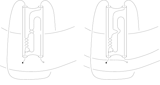
Figure 12. Unwinding full twists of the middle two strands.

Figure 12(a) shows a knot and tunnel produced by a cabling construction, starting from a tunnel in the standard position seen in Figure 5(c). Notice that the original tunnel arc seen in Figure 5(c) now appears as an arc of the new knot— this is the “swap” part of the cabling construction. The arc labeled $\alpha_{W}$ in Figure 5(c), that was an arc of the original knot, is replaced by a standard tangle in the position shown in Figure 12(a). The new tunnel arc is the dotted arc at the lower left of the two-bridge configuration. Provided that the original tunnel arc was the canonical tunnel arc of the original knot, the new tunnel arc is the canonical tunnel arc of the new knot. This is because the cablings in the unique sequence producing a tunnel produce the canonical tunnel arcs for each tunnel (see Section 6).

The knot resulting from this cabling construction depends on the element $\omega\in\mathcal{B}$, not just on its double coset $\langle\delta_{\ell},\sigma\rangle\omega\langle\delta_{m},\sigma\rangle$.

Since the slope of any cabling producing a knot (rather than a two-component link) is of the form $q/p$ with $q$ odd, Lemma 14.2 of [7] shows that $q/p$ has a continued fraction expansion of the form $[2a_{1},b_{1},2a_{2},b_{1},\ldots,\allowbreak 2a_{n},b_{n}]$. So we can and will assume that the standard tangle in Figure 12 has type of the form $(2a_{1},b_{1},2a_{2},\ldots,2a_{n},b_{n})$, and conseqeuntly the middle two strands in the tangle have only full twists.

The first maneuver unwinds one left-hand full twist of the middle two strands at the top of the braid, adding a letter $\delta_{\ell}^{-1}$ at the beginning of the braid description of the previous knot. During the isotopy, the knot cuts once across a core circle of $W$. The resulting knot is shown in Figure 12(b). If the twist is right-hand, the isotopy is similar but a letter $\delta_{\ell}$ is added.

(a) [B] at 260 -15 (b) [B] at 850 -15

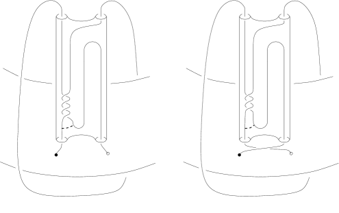
Figure 13. Unwinding half twists of the left two strands.

The second maneuver is possible when there are no twists of the middle two strands at the top of the braid, as in Figures 12(b) and 13(a). It is similar to the first maneuver, but unwinds half twists of the left two strands at the expense of an initial powers of $\sigma$ to $\omega$. During the isotopy, the knot need not pass through a core circle of $W$; it can be fixed outside a small neighborhood of the ball $B$ that contains the standard tangle. As seen in Figure 13(b), unwinding a single half twist adds an initial letter $\sigma$ or $\sigma^{-1}$ to the braid description, according as the half-twist is right-handed or left-handed.

If there are additional twists of the middle or left strands lying below those shown in Figure 12, they can be unwound by repeating the previous two maneuvers. Thus the sequence of full twists of the middle two strands and half twists of the left two strands unwinds to add $\sigma^{b_{n}}\delta_{\ell}^{-a_{n}}\cdots\sigma^{b_{1}}\delta_{\ell}^{-a_{1}}$ at the start of the braid description. The knot and tunnel are then in the position in Figure 5(a), and the maneuver of Section 2 puts the knot and tunnel into the standard position of Figure 5(c), adding $\delta_{m}\sigma$ to the front of the braid description. This establishes our first main result:

Theorem 8.1 (Unwinding Theorem).

Suppose that a $(1,1)$-knot $K$ and its upper $(1,1)$-tunnel are in standard position with braid description $w\in\mathcal{B}$. Perform a cabling construction that introduces a standard tangle of type $(2a_{1},b_{1},\ldots,2a_{n},b_{n})$, positioned as shown in Figure 12. Then using $(1,1)$-isotopy, the new knot and tunnel can be put into standard position with braid description

$$\delta_{m}\sigma\cdot\sigma^{b_{n}}\delta_{\ell}^{-a_{n}}\sigma^{b_{n-1}}\cdots\sigma^{b_{1}}\delta_{\ell}^{-a_{1}}\cdot w\ .$$

9. The Slope Theorem

To calculate the slope invariant of a cabling as in Figure 12, we must first find the slope-zero perpendicular disk $\rho^{0}$ of $\rho$, where $\rho$ is the slope disk in Figure 14 (a). Then we determine the $\{\rho,\rho^{0}\}$-slope of the standard tangle of type $(2a_{1},b_{1},\ldots,2a_{n},b_{n})$. In this section, we will carry these out, leading to our second main result, Theorem 9.3. It gives a simple expression for the slope of a cabling construction of the type considered in Theorem 8.1. The expression involves an integer that counts the number of turns the knot makes around the solid torus $T\times I\cup V$. Definition 9.1 and Proposition 9.2 will show how to compute this integer from a braid description of the $(1,1)$-position.

$\rho$ [B] at 261 310 $t$ times [B] at 470 160 (a) [B] at 264 0 (b) [B] at 841 0

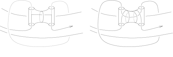
Figure 14. Finding the slope-zero perpendicular disk $\rho^{0}$. The first drawing shows $\rho$ and indicates the direction of algebraically positive winding of the knot around $V$. The second shows the $0$-linking pair for $\rho^{0}$, for the case $t=3$. The corresponding disk $\rho^{0}$ appears in Figure 15(b).

Assuming that the upper tunnel of $K$ is in standard position as in Figure 5(c), we always choose the orientation on $K$ to be directed over the top arch $\alpha_{W}$ from the black point to the white point. The algebraic winding number for this position of $K$ is defined to be the net number of turns that $K$ makes in the direction of positive orientation on the longitude $\ell$ of $T\times I\cup V$ (the direction indicated in Figure 14(a)), that is, the algebraic intersection of $K$ with a meridian disk of $T\times I\cup V$ bounded by the loop $m$.

Definition 9.1.

For $\omega\in\mathcal{B}$, define $t(\omega)\in\operatorname{{\mathbb{Z}}}$ as follows. For each appearance of $\delta_{\ell}^{\epsilon}$ ($\epsilon=\pm 1$) in $\omega$, write $\omega=\omega_{1}\delta_{\ell}^{\epsilon}\omega_{2}$, and let $k$ be the total exponent of $\sigma$ in $\omega_{1}$. Assign the value $(-1)^{k+1}\epsilon$ to this appearance of $\delta_{\ell}^{\epsilon}$, and sum these over all appearances to give $t(\omega)$.

Proposition 9.2.

If $K=K(\omega)$, then $t(\omega)$ equals the algebraic winding number of $K$.

Proof.

For our designated orientation on $K$ and choice of direction of positive winding, an initial letter $\delta_{\ell}$ in $\omega$ as in the example of Figure 3(a) would contribute $-1$ to the algebraic winding number of $K$. If it were $\delta_{\ell}^{-1}$ it would contribute $+1$. When $\delta_{\ell}^{\epsilon}$ is not the initial letter, each of the appearances of $\sigma$ preceding an appearance of $\delta_{\ell}^{\epsilon}$ in $\omega$ reverses the direction in which the orientation of $K$ is directed around the turn corresponding to this $\delta_{\ell}^{\epsilon}$ term. So if there are $k$ such appearances of $\sigma$, this appearance of $\delta_{\ell}^{\epsilon}$ contributes $(-1)^{k}(-\epsilon)=(-1)^{k+1}\epsilon$ to the algebraic winding number. Apart from this effect of $\sigma$ on the signs of these terms, the appearances of $\delta_{m}$ and $\sigma$ in $\omega$ make no contribution to the algebraic winding number. ∎

We can now state our second main result.

Theorem 9.3 (Slope Theorem).

Let $K=K(\omega)$ be a knot in braid position with upper tunnel in standard position as shown in Figure 5(c). Suppose that a cabling construction as in Figure 12 is performed using a standard tangle of type $(2a_{1},b_{1},\ldots,2a_{n},b_{n})$. Then the slope of the cabling is given by the continued fraction $[2t(\omega)+2a_{1},b_{1},2a_{2},\ldots,b_{n}]$.

Proof.

Figure 14(b) shows the link formed by the core circles of the solid tori into which the slope disk in Figure 15(b) will cut a handlebody neighborhood of the union of the knot and the tunnel. The lower component is $(1,1)$-isotopic to $K$, while the upper component is a core circle of the solid torus $W$. Let $t$ be the number of full left-handed twists of the right half of $B$ needed to change the disk $\rho^{\perp}$ in Figure 15(a) to the disk in Figure 15(b). Recalling that the algebraic winding number of $K$ is its algebraic intersection number with a meridian disk of $T\times I\cup V$, we see that the linking number of the lower component with the upper component is $t$ less than the algebraic winding number of $K$. If we choose $t$ to equal this algebraic winding number, then the linking number will be $0$, and therefore the disk in Figure 15(b) will be the canonical zero-slope disk $\rho^{0}$. According to Proposition 9.2, the algebraic winding number of $K$ is $t(\omega)$, so the condition is that $t=t(\omega)$.

$\tau_{+}$ [B] at -11 136 $\tau_{-}$ [B] at 180 136 $\tau_{+}$ [B] at 245 136 $\tau_{-}$ [B] at 435 136 $\rho$ [B] at 82 126 $\rho^{\bot}$ [B] at 180 80 $\rho^{0}$ [B] at 435 70 $\lambda_{+}$ [B] at -11 30 $\lambda_{-}$ [B] at 180 30 $\lambda_{+}$ [B] at 245 30 $\lambda_{-}$ [B] at 435 30 (a) [B] at 85 0 (b) [B] at 340 0

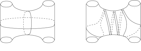
Figure 15. A perpendicular disk $\rho^{\perp}$ and the slope-zero perpendicular disk $\rho^{0}$ for the case $t=3$.

Now consider a standard tangle $K_{0}$ of type $(2a_{1},b_{1},\ldots,2a_{n},b_{n})$, as shown in Figure 10. Regard it as contained in the portion of the handlebody shown in Figure 15, as in Figure 12. Proposition 7.1 gives the slope of $K_{0}$ with respect to the pair $\{\rho,\rho^{\perp}\}$ in Figure 15(a) to be $[2a_{1},b_{1},\ldots,2a_{n},b_{n}]$. We denote this slope by $m(K_{0},\{\rho,\rho^{\perp}\})$, and by $m(K_{0},\{\rho,\rho^{0}\})$ the slope with respect to $\{\rho,\rho^{0}\}$.

Let $u$ denote a full left-hand twist of the right-hand side of the ball in Figure 15. We have already seen that $u^{t}(\rho^{\perp})=\rho^{0}$, and we note also that $u^{t}(\rho)=\rho$. In the view of Figure 10, $u$ is a full left-hand twist of the bottom half of $B$, so $u^{-t}$ moves $K_{0}$ to the standard tangle of type $(2t+2a_{1},b_{1},2a_{2},b_{2},\ldots,2a_{n},b_{n})$. We can now compute the slope of the cabling as

$$m(K_{0},\{\rho,\rho^{0}\})=m(K_{0},\{\rho,u^{t}(\rho^{\perp})\})=m(K_{0},\{u^{t}(\rho),u^{t}(\rho^{\perp})\})$$

$$=m(u^{-t}(K_{0}),\{\rho,\rho^{\perp}\})=[2t+2a_{1},b_{1},\ldots,2a_{n},b_{n}]$$

where Proposition 7.1 gives the final equality. ∎

Example 9.4.

Figure 16 shows the knot of Figure 9 of [7] moved into $(1,1)$-position. The upper right-hand drawing is the original knot and its upper and lower tunnels $\tau_{1}$ and $\tau_{2}$. In the $(1,1)$-position in Figure 9 of [7], $\tau_{2}$ is the upper tunnel. From the bottom-right drawing, we read off a braid description of $\tau_{2}$ as $\omega=\delta_{m}^{-1}\sigma^{-1}\delta_{\ell}\delta_{m}^{-1}\sigma^{3}\delta_{\ell}^{-1}=\sigma\delta_{m}\delta_{\ell}\delta_{m}^{-1}\sigma^{3}\delta_{\ell}^{-1}\sim\delta_{m}\delta_{\ell}\delta_{m}^{-1}\sigma^{3}\delta_{\ell}^{-1}$.

$\tau_{1}$ [B] at 66 128 $\tau_{2}$ [B] at 66 188 $\tau_{1}$ [B] at 194 153 $\tau_{2}$ [B] at 223 176 $\tau_{1}$ [B] at 60 17 $\tau_{2}$ [B] at 61 70 $\tau_{1}$ [B] at 200 12 $\tau_{2}$ [B] at 199 75

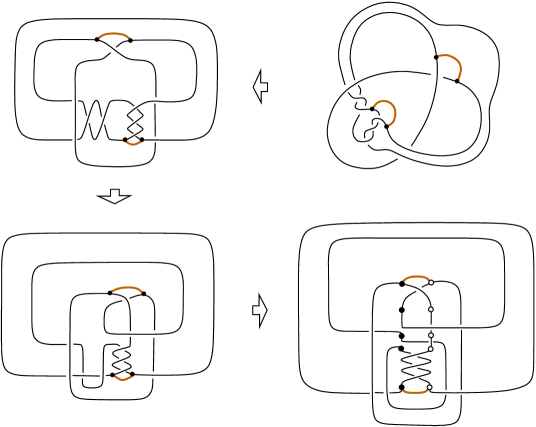
Figure 16. Putting a knot into $(1,1)$-position

To compute the slope invariants for the tunnel $\tau_{2}$, we use the relation $\delta_{m}^{-1}=\sigma\delta_{m}\sigma$ to put $\omega$ into the form

$$\delta_{m}\sigma\cdot\omega_{1}(\delta_{\ell},\sigma)\cdot\delta_{m}\sigma\cdot\omega_{0}(\delta_{\ell},\sigma)=\delta_{m}\sigma\cdot\sigma^{-1}\delta_{\ell}\sigma\cdot\delta_{m}\sigma\cdot\sigma^{3}\delta_{\ell}^{-1}\ .$$

We now use Theorems 8.1 and 9.3 to read off the slopes. The first cabling starts from the trivial knot $K$, which has algebraic winding number $t(1)=0$. Since the cabling corresponds to the portion $\delta_{m}\sigma\cdot\omega_{0}(\delta_{\ell},\sigma)=\delta_{m}\sigma\cdot\sigma^{3}\delta_{\ell}^{-1}$, Theorem 8.1 shows that the standard tangle used in the cabling is of type $(2a_{1},b_{1})=(2,3)$. By Theorem 9.3, the ordinary slope of the first cabling is given by the continued fraction $[0+2,3]=7/3$, so the simple slope is $[3/7]$ in $\operatorname{{\mathbb{Q}}}/\operatorname{{\mathbb{Z}}}$. The second cabling begins with this knot, so has algebraic winding number $t(\delta_{m}\sigma\cdot\sigma^{3}\delta_{\ell}^{-1})=(-1)^{4+1}\cdot(-1)=1$. From Theorem 8.1, we have $a_{1}=0$, $b_{1}=1$, $a_{2}=-1$, and $b_{2}=-1$, so by Theorem 9.3 the second cabling slope is given by the continued fraction $[2+0,1,-2,-1]=7/2$. Therefore the slope sequence of $\tau_{2}$ is $[3/7],7/2$.

The tunnel $\tau_{1}$ is the upper tunnel of the $(1,1)$-position described by the reverse braid of $\omega$,

$$\delta_{m}^{-1}\sigma^{3}\delta_{\ell}^{-1}\delta_{m}\delta_{\ell}\sim\delta_{m}\sigma\cdot\sigma^{3}\delta_{\ell}^{-1}\cdot\delta_{m}\sigma\cdot\sigma^{-1}\delta_{\ell}\ ,$$

giving the first slope of $\tau_{1}$ to be $[0+(-2),-1]=-3$ and consequently its simple slope to be $[-1/3]=[2/3]\in\operatorname{{\mathbb{Q}}}/\operatorname{{\mathbb{Z}}}$. For the second slope, we have $t(\delta_{m}\delta_{\ell})=(-1)^{0+1}\cdot 1=-1$, $a_{1}=1$, and $b_{1}=3$, giving the slope $[2\cdot(-1)+2,3]=1/3$. Therefore the cabling slope sequence of the lower tunnel is $[2/3],1/3$.

10. Tunnels of $2$-bridge knots

In this section we will give braid descriptions of the tunnels of $2$-bridge knots, and use them to calculate the slope invariants. We obtain, of course, the same values as in the calculation of [7, Section 15]. In Theorem 10.5 we give a characterization of which sequences of rational numbers (with initial term in $\operatorname{{\mathbb{Q}}}/\operatorname{{\mathbb{Z}}}$) occur as slope sequences of tunnels of $2$-bridge knots.

A convenient reference for the tunnels of $2$-bridge knots is K. Morimoto and M. Sakuma [15, Section (1.6)]. In [15, Section (1.1)], the authors give a definition of dual tunnels, and the discussion in [15, Section (1.2)] shows that two tunnels of a knot in $S^{3}$ are dual exactly when they are the upper and lower tunnels for the same $(1,1)$-position of the knot. As we saw in Section 1, the dual of a tunnel given by a braid description $\omega$ has a braid description by the reverse braid of $\omega$.

$U$ [B] at -10 45 $US$ [B] at 66 83 $L$ [B] at 376 50 $LS$ [B] at 354 78 $2a_{1}$ [B] at 100 45 $2a_{2}$ [B] at 198 45 $b_{1}$ [B] at 150 12 $b_{n}$ [B] at 335 12

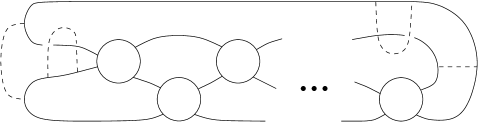
Figure 17. A $2$-bridge knot with classifying invariant given by the continued fraction $1/[2a_{1},b_{1},2a_{2},\ldots,2a_{n},b_{n}]$. The upper and lower tunnels $U$ and $L$ and the upper and lower semisimple tunnels $US$ and $LS$ are shown.

Figure 17 shows a $2$-bridge knot, where the regions labeled $2a_{i}$ indicate $2a_{i}$ left-hand half-twists and those labeled $b_{i}$ indicate $b_{i}$ right-hand half-twists. The upper, lower, upper semisimple, and lower semisimple tunnels are shown; from [15, Section (1.6)], the upper semisimple and lower simple tunnels are dual, as are the lower semisimple and upper simple tunnels.

This position is assigned to the rational number $a/b$ given by the continued fraction $[2a_{1},b_{1},2a_{2},\ldots,2a_{n},b_{n}]$. Changing the position by $(1,1)$-isotopy if need be, we may assume that $2a_{1}$ and $b_{n}$ are nonzero (indeed we may assume that no $a_{i}$ or $b_{i}$ is zero, although for some calculations it is convenient to allow zero values), and we always choose $a$ positive, so have $0<|b|<a$. Also, $a$ is odd (the values when $a$ is even correspond to $2$-bridge links).

Notice that there is an isotopy moving the knot in Figure 17 to the position given by the continued fraction $[-b_{n},-2a_{n},-b_{n-1},\ldots,-b_{1},-2a_{1}]$. The first step is to move the top horizontal strand down to the bottom. The twists $b_{i}$ then appear in the middle and the $2a_{i}$ at the top. Then the entire knot is rotated until it looks as in Figure 17 except with the twists $b_{i}$ in the middle and the $2a_{i}$ at the bottom; the minus signs are due to the convention about which directions of twists are considered to be positive for the middle versus the bottom two strands. The upper tunnel for the second position is the lower tunnel for the original position. Similarly, the upper semisimple tunnel for the first position is the lower semisimple tunnel for the second.

If $[2a_{1},b_{1},\ldots,2a_{n},b_{n}]=a/b$, then $[-b_{n},-2a_{n},-b_{n-1},\ldots,-b_{1},-2a_{1}]$ is $a/b^{\prime}$ where $0<|b|<a$, $0<|b^{\prime}|<a$, and $bb^{\prime}\equiv 1\bmod a$. This and many other basic facts about continued fraction expansions can be verified using [7, Lemma 14.3]. For suppose we use Lemma 14.2 of [7] (which is itself a consequence of Lemma 14.3 of [7]) to write $[2a_{1},b_{1},\ldots,2a_{n},b_{n}]=a/b$. By Lemma 14.3 of [7], we have $U^{2a_{1}}L^{b_{1}}\cdots U^{2a_{n}}L^{b_{n}}=\begin{bmatrix}a&r\\ b&s\end{bmatrix}$ where $[-b_{n},-2a_{n},-b_{n-1},\ldots,-b_{1},-2a_{1}]=-[b_{n},2a_{n},b_{n-1},\ldots,b_{1},2a_{1}]=a/(-r)$. Since $as-rb=1$, we have $(-r)b=1\bmod a$.

The $2$-bridge knot is actually classified up to isotopy by the pair of (possibly equal) values $b/a$ and $b^{\prime}/a$ in $\operatorname{{\mathbb{Q}}}/\operatorname{{\mathbb{Z}}}$. Replacing $a/b$ by $a/(b\pm a)$, if necessary, and applying Lemma 14.2 of [7], we may assume that all terms in the continued fraction expansion of $a/b$ are even. The corresponding $2$-bridge position, having only full twists of the left two strands and the middle two strands, is called the Conway position of the $2$-bridge knot.

Proposition 10.1.

The lower simple tunnel has slope invariant

$$m_{0}=[1/[2a_{1},b_{1},\ldots,2a_{n},b_{n}]]\ ,$$

and the upper simple tunnel has slope invariant

$$m_{0}=[1/[-b_{n},-2a_{n},-b_{n-1},\ldots,-b_{1},-2a_{1}]]\ .$$

Proof.

Figure 18, a case of Figure 12(a), shows a $2$-bridge knot $K$ obtained from the trivial knot $K_{0}$ by a single cabling. The tunnel arc is the lower simple tunnel of $K$. Since the algebraic winding number $t(K_{0})$ is $0$, Theorem 9.3 gives the slope of this cabling to be $[2a_{1},b_{1},\ldots,2a_{n},b_{n}]$, so the simple slope of the lower tunnel is $[1/[2a_{1},b_{1},\ldots,2a_{n},b_{n}]]$. Since the upper simple tunnel is the lower simple tunnel for the position of $K$ corresponding to the continued fraction $[-b_{n},-2a_{n},-b_{n-1},\ldots,-b_{1},-2a_{1}]$, the simple slope of the upper tunnel is as given in the proposition. (To apply Theorem 9.3, the position would have to be moved by isotopy to change the $-b_{i}$ to be even, but this would not change the value of the continued fraction.)

$2a_{1}$ [B] at 300 370 $b_{1}$ [B] at 247 280

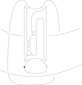
Figure 18. The slope calculation for the lower tunnel of a $2$-bridge knot.

∎

From Proposition 10.1, we have

Corollary 10.2.

Let the rational invariant of the $2$-bridge knot be given by the continued fraction $a/b=[2a_{1},b_{1},2a_{2},\ldots,2a_{n},b_{n}]$, with $0<b<a$. Let $b^{\prime}$ be the integer with $0<b^{\prime}<a$ and $bb^{\prime}\equiv 1\mod a$. Then the simple slope of the upper tunnel of $K$ is $[b^{\prime}/a]$, and the simple slope of the lower tunnel is $[b/a]$.

We turn now to the semisimple tunnels, whose slope invariants were calculated in [7]. We will obtain a braid description such that the upper semisimple tunnel is the upper tunnel for the associated $(1,1)$-position, then use it to recover the slope calculation of [7]. We will also prove a new result, Theorem 10.5, which characterizes the slope sequences of these tunnels.

Braid descriptions of these $(1,1)$-positions were given by A. Cattabriga and M. Mulazzani [4] and more recently in the dissertation of A. Seo [18]. Here is the braid description that we will use:

Lemma 10.3.

The braid word $\delta_{m}^{-a_{1}}\sigma^{b_{1}}\cdots\delta_{m}^{-a_{n}}\sigma^{b_{n}}\delta_{\ell}^{-1}$ describes a $(1,1)$-position of the $2$-bridge knot $K$ given by $[2a_{1},b_{1},\ldots,2a_{n},b_{n}]$. The upper tunnel of this $(1,1)$-position is the upper semisimple tunnwl of $K$.

A quick way to obtain this braid description is to use the fact that the upper semisimple tunnel is dual to the lower simple tunnel. As seen in Figure 18, the lower simple tunnel is obtained from the upper tunnel of the trivial knot by a single cabling of type $(2a_{1},b_{1},\ldots,2a_{n},b_{n})$. By Theorem 8.1, this $(1,1)$-position is described by the braid $\delta_{m}\sigma^{b_{n}+1}\delta_{\ell}^{-a_{n}}\cdots\sigma^{b_{1}}\delta_{\ell}^{-a_{1}}$. Since the upper semisimple tunnel is dual to the lower simple tunnel, it is the upper tunnel of the $(1,1)$-position described by the reverse of this word, which is

$$\delta_{m}^{-a_{1}}\sigma^{b_{1}}\cdots\delta_{m}^{-a_{n}}\sigma^{b_{n}+1}\delta_{\ell}\sim\delta_{m}^{-a_{1}}\sigma^{b_{1}}\cdots\delta_{m}^{-a_{n}}\sigma^{b_{n}}\delta_{\ell}^{-1}\ .$$

$m$ [B] at 203 415 $\ell$ [B] at 180 350 $\delta^{-1}_{m}$ [B] at 315 130 $\sigma$ [B] at 137 35 $\ell$ [B] at 573 262 $m$ [B] at 655 195

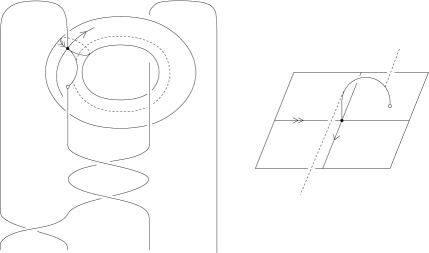
Figure 19. Calculation of the braid description for the upper semisimple tunnel of a $2$-bridge knot, as seen from the outside and from the inside of the standard torus.

$m$ [B] at 198 305 $\ell$ [B] at 180 241

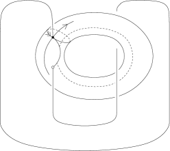
Figure 20. The initial position of the trivial tunnel as an upper semisimple tunnel has braid description $\delta_{\ell}^{-1}$.

A second, perhaps more satisfying way to obtain Lemma 10.3 is to see the braid directly. Figure 19 shows the setup. The second drawing shows the view from inside $W$, similar to the view of Figure 3, and the first shows the view from $T\times I$ looking at $W$ from the outside. Observe that a full twist of the middle two strands represents the braid that moves the white point around $m$ in the positive direction, which is $\delta_{m}^{-1}$, and the half twist of the left two strands represents $\sigma$.

Figure 20 shows the tunnel of the trivial knot as the upper semisimple tunnel of the trivial $2$-bridge knot. It is the upper tunnel for the $(1,1)$-position of the trivial knot described by the braid $\delta_{\ell}^{-1}$ that moves the white point around $\ell$ in the positive direction, that is, $K(\delta_{\ell}^{-1})$.

Now, modify the trivial knot in Figure 20 by inserting a standard tangle of type $(2a_{1},b_{1},\ldots,2a_{n},b_{n})$ into $T\times I$, in the position seen in Figure 19. The portion labeled $\delta_{m}^{-1}$ in Figure 19 will be $2a_{1}$ left-hand half twists, the portion labeled $\sigma$ will be $b_{1}$ right-hand half twists, below this will be $2a_{2}$ left-hand half twists, and so on, ending with $b_{n}$ half twists and then the $\delta_{\ell}^{-1}$ already present. This produces the knot seen in Figure 17, and the upper semisimple tunnel seen there, and the braid description of Lemma 10.3.

We are now ready to calculate the slope invariants. By allowing the possibility that $b_{i}=0$, we may assume that every $a_{i}$ is $\pm 1$ (since continued fractions have the property that $[\cdots,n_{1}+n_{2},\cdots]=[\cdots,n_{1},0,n_{2},\cdots]$). We may further assume that if the last term $b_{n}=\pm 1$ then $a_{n}$ and $b_{n}$ have the same sign.

It is convenient to reindex the continued fraction as $[2a_{d},b_{d},2a_{d-1},\ldots,\allowbreak 2a_{0},b_{0}]$. We first consider four cases with $i\geq 1$:

Case I: $a_{i}=1$, $a_{i-1}=1$

In this case the braid appears as

$$\omega_{1}\;\delta_{m}^{-1}\sigma^{b_{i}}\;\delta_{m}^{-1}\sigma^{b_{i-1}}\;\omega_{2}=\omega_{1}\;\sigma\;(\delta_{m}\sigma)\sigma^{b_{i}+1}\;\delta_{m}\sigma^{b_{i-1}+1}\;\omega_{2}$$

and the cabling corresponding to $a_{i}$ has slope $[2t(\omega),b_{i}+1]$, where $\omega=\delta_{m}\sigma^{b_{i-1}+1}\;\omega_{2}$.

Case II: $a_{i}=-1$, $a_{i-1}=1$

The braid is

$$\omega_{1}\;\delta_{m}\sigma^{b_{i}}\;\delta_{m}^{-1}\sigma^{b_{i-1}}\;\omega_{2}=\omega_{1}\;(\delta_{m}\sigma)\sigma^{b_{i}}\;\delta_{m}\sigma^{b_{i-1}+1}\;\omega_{2}$$

and the cabling corresponding to $a_{i}$ has slope $[2t(\omega),b_{i}]$, where again $\omega=\delta_{m}\sigma^{b_{i-1}+1}\;\omega_{2}$.

Case III: $a_{i}=1$, $a_{i-1}=-1$

The braid is

$$\omega_{1}\;\delta_{m}^{-1}\sigma^{b_{i}}\;\delta_{m}\sigma^{b_{i-1}}\;\omega_{2}=\omega_{1}\;\sigma\;(\delta_{m}\sigma)\sigma^{b_{i}}\;\delta_{m}\sigma^{b_{i-1}}\;\omega_{2}$$

and the cabling corresponding to $a_{i}$ has slope $[2t(\omega),b_{i}]$, but this time $\omega=\delta_{m}\sigma^{b_{i-1}}\;\omega_{2}$.

Case IV: $a_{i}=-1$, $a_{i-1}=-1$

The braid is

$$\omega_{1}\;\delta_{m}\sigma^{b_{i}}\;\delta_{m}\sigma^{b_{i-1}}\;\omega_{2}=\omega_{1}\;(\delta_{m}\sigma)\sigma^{b_{i}-1}\;\delta_{m}\sigma^{b_{i-1}}\;\omega_{2}$$

and the cabling corresponding to $a_{i}$ has slope $[2t(\omega),b_{i}-1]$, where again $\omega=\delta_{m}\sigma^{b_{i-1}}\;\omega_{2}$.

For the initial cabling, we have

Case V: $a_{0}=1$

The braid is

$$\cdots\sigma^{b_{1}}\,\delta_{m}^{-1}\sigma^{b_{0}}\delta_{\ell}^{-1}=\cdots\sigma^{b_{1}+1}\,(\delta_{m}\sigma)\sigma^{b_{0}}\;\delta_{\ell}^{-1}$$

and the initial cabling has simple slope $[1/[2,b_{0}]]=[b_{0}/(2b_{0}+1)]$

Case VI: $a_{0}=-1$

The braid is

$$\cdots\sigma^{b_{1}}\,\delta_{m}\sigma^{b_{0}}\delta_{\ell}^{-1}=\cdots\sigma^{b_{1}}\,(\delta_{m}\sigma)\sigma^{b_{0}-1}\;\delta_{\ell}^{-1}$$

and the initial cabling has simple slope $[1/[2,b_{0}-1]]=[(b_{0}-1)/(2b_{0}-1)]$.

From Cases V and VI, we have $m_{0}=[b_{0}/(2b_{0}+1)]$ or $m_{0}=[(b_{0}-1)/(2b_{0}-1)]$ according as $a_{0}$ is $1$ or $-1$.

To compute the remaining $m_{i}$, we assume that the knot is in Conway position so that all the $b_{i}$ are even. We then have

$$t(\omega_{2})=t(\delta_{m}^{-a_{i-2}}\sigma^{b_{i-2}}\cdots\delta_{m}^{-a_{0}}\sigma^{b_{0}}\delta_{\ell}^{-1})=(-1)^{b_{i-2}+\cdots+b_{0}}=1\ ,$$

and from Cases I-IV, using the fact that $b_{i-1}$ is even, $t(\omega)$ equals $-1$ when $a_{i-1}=1$ and $1$ when $a_{i-1}=-1$. That is, $t(\omega)=-a_{i-1}$. Summarizing, we have

Proposition 10.4.

Let $K$ be in the $2$-bridge position corresponding to the continued fraction $[2a_{d},2b_{d},\ldots,2a_{0},2b_{0}]$, with $b_{0}\neq 0$ and each $a_{i}=\pm 1$. Then the slope invariants of the upper semisimple tunnel of $K$ are as follows:

1. $m_{0}=\left[\displaystyle\frac{2b_{0}}{4b_{0}+1}\right]$ or $m_{0}=\left[\displaystyle\frac{2b_{0}-1}{4b_{0}-1}\right]$ according as $a_{0}$ is $1$ or $-1$.

2. For $1\leq i\leq d$, $m_{i}=-2a_{i-1}+1/k_{i}$, where

   1. $k_{i}=2b_{i}+1$ if $a_{i}=a_{i-1}=1$,

   2. $k_{i}=2b_{i}$ if $a_{i}$ and $a_{i-1}$ have opposite signs, and

   3. $k_{i}=2b_{i}-1$ if $a_{i}=a_{i-1}=-1$.

This agrees with the calculation obtained in [7, Section 15].

Using Proposition 10.4, we can characterize the slope sequences of semisimple tunnels of $2$-bridge knots.

Theorem 10.5.

Let $m_{0},m_{1},\ldots\,$, $m_{d}$ be a sequence with $m_{0}\in\operatorname{{\mathbb{Q}}}/\operatorname{{\mathbb{Z}}}$ and $m_{i}\in\operatorname{{\mathbb{Q}}}$ for $i>0$. Then $m_{0},m_{1},\ldots\,$, $m_{d}$ is the slope sequence for a semisimple tunnel of a $2$-bridge knot if and only if it satisfies the following:

1. $m_{0}=\left[\displaystyle\frac{n_{0}}{2n_{0}+1}\right]$ for some $n_{0}\notin\{-1,0\}$.

2. For $i>0$, $m_{i}=\pm 2+\displaystyle\frac{1}{k_{i}}$ for some integer $k_{i}\neq 0$.

3. $m_{1}$ is positive or negative according as $n_{0}$ is odd or even.

4. For $1\leq i\leq d$, $m_{i}$ has the same sign as $m_{i-1}$ if and only if $k_{i-1}$ is odd.

Proof.

First assume that this is a slope sequence for a semisimple tunnel. Part (i) follows from Proposition 10.4(i), with the excluded cases corresponding to the cases when $b_{0}=0$. Part (ii) is immediate from Proposition 10.4(ii). In Proposition 10.4(ii), $m_{1}$ has the opposite sign from $a_{0}$, and Proposition 10.4(i) shows that $a_{0}$ is negative or positive according as $n_{0}$ is odd or even. This establishes part (iii). For part (iv), Proposition 10.4(ii) shows that the signs of $m_{i}$ and $m_{i-1}$ differ exactly when $a_{i-1}$ and $a_{i-2}$ have opposite signs. By Proposition 10.4(ii)(a)(b)(c), this is exactly the case when $k_{i-1}=2b_{i-1}$, and when $a_{i-1}$ and $a_{i-2}$ have the same sign, $k_{i-1}=2b_{i-1}\pm 1$ which is odd.

For the converse, given a sequence $m_{0},\ldots\,$, $m_{d}$ as in the statement of the Proposition, we will construct the continued fraction expansion $a/b=[2a_{d},2b_{d},\ldots,2a_{0},2b_{0}]$ for the Conway position, with each $a_{i}=\pm 1$. Let $a_{0}$ be $-1$ or $1$ according to whether $n_{0}$ is odd or even. For ascending $i$ with $1\leq i\leq d$, let $a_{i}$ be $a_{i-1}$ if $k_{i}$ is odd, and $-a_{i-1}$ if it is even. For the $b_{i}$, put $2b_{0}=n_{0}$ or $n_{0}+1$ according as $n_{0}$ is even or odd. Cases I-IV now determine the choices of the remaining $2b_{i}$ which produce the correct values for the $m_{i}$: When $a_{i}=-a_{i-1}$, $k_{i}$ is even and Cases II and III give $2b_{i}=k_{i}$. When $a_{i}=a_{i-1}$, $k_{i}$ is odd and Cases I and IV show that $2b_{i}=k_{i}-1$ if $a_{i}=1$ and $2b_{i}=k_{i}+1$ if $a_{i}=-1$. ∎

11. Semisimple tunnels of torus knots

To set notation, consider a (nontrivial) $(p,q)$-torus knot $K_{p,q}$, contained in our standard torus $T$. It represents $p$ times a generator in $\pi_{1}(V\cup T\times I)$, and $q$ times a generator in $\pi_{1}(W)$.

The tunnels of torus knots were classified by M. Boileau, M. Rost, and H. Zieschang [3] and Y. Moriah [14]. The middle tunnel of $K_{p,q}$ is represented by an arc in $T$ that meets $K_{p,q}$ only in its endpoints. The upper tunnel of $K_{p,q}$ is represented by an arc $\alpha$ properly imbedded in $W$, such that the circle which is the union of $\alpha$ with one of the two arcs of $K_{p,q}$ with endpoints equal to the endpoints of $\alpha$ is a deformation retract of $W$. The lower tunnel is like the upper tunnel, but interchanging the roles of $V\cup T\times I$ and $W$. For some choices of $p$ and $q$, some of these tunnels are equivalent.

A braid description for torus knots was obtained by A. Cattabriga and M. Mulazzani [5, Section 4]. Here we will use a similar description due to A. Seo [18]. Fix $(p,q)$ relatively prime, and suppose for now that $p,q\geq 2$. In $\operatorname{{\mathbb{R}}}^{2}$ we construct a polygonal path $P_{p,q}$ from $(0,0)$ to $(p,q)$, as indicated in Figure 21 for the cases when $(p,q)$ is $(3,7)$ and $(7,3)$, as follows: Regard $\operatorname{{\mathbb{R}}}^{2}$ as made up of squares with side length $1$, whose corners have integer coordinates. Consider the rectangle $R$ with corners $(0,0)$ and $(p,q)$, and let $S$ be the union of the squares in $\operatorname{{\mathbb{R}}}^{2}$ whose bottom sides contain no points above the line containing $(0,0)$ and $(p,q)$. Then $P_{p,q}$ is $R\cap\partial S$.

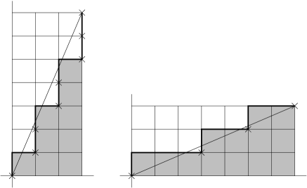
Figure 21. The points $(p_{k},k)$ for $0\leq k\leq q$ for the cases $(p,q)=(3,7)$ and $(p,q)=(7,3)$.

Explicitly, for $0\leq k\leq q$ put $p_{k}=\lceil kp/q\rceil$. The points $(p_{k},k)$ are indicated in Figure 21. The intersection point of the diagonal of $R$ with the line $y=k$ has $x$-coordinate $kp/q$, so $\lceil kp/q\rceil$ is the $x$-coordinate of the first integral lattice point on $y=k$ that lies on or to the right of this intersection point. The path $P_{p,q}$ is the union for $1\leq i\leq q$ of the segments (some of which may have length $0$) from $(p_{i-1},i-1)$ to $(p_{i-1},i)$ and from $(p_{i-1},i)$ to $(p_{i},i)$.

We will now use $P_{p,q}$ to obtain a braid description of $K_{p,q}$. As usual, the braid portion will start in $T$. Referring again to Figure 21, we may assume that the plane picture is drawn so that the lifts of the fixed arc $\alpha$ in $T$ from the black point to the white point are short straight line segments positioned so that each meets only the translate of the diagonal of $R$ that contains its lower left point (that is, its black point), and apart from that point lies below that translate.

Consider the braid $\beta$ with the following description. As we descend in $T\times I$, the $T$-coordinate of the white point stays fixed, while the $T$-coordinate of the black point moves backward along the $(p,q)$-curve which is the image of the diagonal of the rectangle (that is, the lift to $\operatorname{{\mathbb{R}}}^{2}$ of its path in $T$ starting $(p,q)$ travels along the diagonal of $R$ to $(0,0)$). The choice of the backward direction is not essential, but leads to a simpler calculation. Since each lift of $\alpha$ lie below the translate of the diagonal that it meets, the diagonal of $R$ is isotopic, not crossing any lift of $\alpha$ and in particular not crossing any lift of the white point, to $P_{p,q}$. This implies that $\beta$ is represented by the braid word whose letters correspond to the horizontal and vertical steps along $P_{p,q}$ (starting from the upper right), with each downward step being $\delta_{m}$ and each leftward step being $\delta_{\ell}^{-1}$. This word is

$$\omega_{(p,q)}=\delta_{\ell}^{p_{q-1}-p_{q}}\delta_{m}\;\cdots\;\delta_{\ell}^{p_{0}-p_{1}}\delta_{m}\ .$$

Similar considerations give a braid description for the case when $p>0$ and $q<0$. For $0\leq k\leq p$ put $q_{k}=\lceil kq/p\rceil$. The braid is then $\omega_{(p,q)}=\prod_{k=0}^{p-1}\delta_{\ell}\delta_{m}^{q_{k}-q_{k+1}}$.

Assuming as before that $p,q\geq 2$, we now use $\omega_{(p,q)}$ to compute the slope coefficients of the upper tunnel of $K_{p,q}$. We have

$$\omega_{(p,q)}\sim\delta_{m}\delta_{\ell}^{p_{q-2}-p_{q-1}}\;\cdots\;\delta_{m}\delta_{\ell}^{p_{1}-p_{2}}\;\delta_{m}\delta_{\ell}^{p_{0}-p_{1}}$$

$$=\delta_{m}\sigma\;\sigma^{-1}\delta_{\ell}^{p_{q-2}-p_{q-1}}\;\cdots\;\delta_{m}\sigma\;\sigma^{-1}\delta_{\ell}^{p_{1}-p_{2}}\;\delta_{m}\sigma\;\sigma^{-1}\delta_{\ell}^{p_{0}-p_{1}}\ .$$

Putting $\omega_{j}=\delta_{m}\delta_{\ell}^{p_{j-1}-p_{j}}\;\cdots\;\delta_{m}\delta_{\ell}^{p_{1}-p_{2}}\;\delta_{m}\delta_{\ell}^{-p_{1}}$, we have

$$t(\omega_{j})=(p_{j}-p_{j-1})+\cdots+(p_{2}-p_{1})+(p_{1}-p_{0})=p_{j}-p_{0}=p_{j}\ .$$

Now, working from the right, Theorem 9.3 finds the cabling slope sequence for the upper tunnel:

$$[2(p_{1}-p_{0}),-1]=2p_{1}-1$$

$$[2t(\omega_{1})+2(p_{2}-p_{1}),-1]=2p_{2}-1$$

$$\cdots$$

$$[2t(\omega_{q-2})+2(p_{q-1}-p_{q-2}),-1]=2p_{q-1}-1$$

These give the trivial knot as long as $p_{j}\leq 1$, so we have reproved one of the main results from [8]:

Theorem 11.1.

Let $p$ and $q$ be relatively prime integers, both greater than $1$. For $1\leq k\leq q$, put $p_{k}=\lceil kp/q\rceil$, and let $k_{0}=\min\{k\;|\;p_{k}>1\}$. Then the upper tunnel of $K_{p,q}$ is produced by $q-k_{0}$ cabling constructions, whose slopes are

$$[1/(2p_{k_{0}}-1)],\;2p_{k_{0}+1}-1,\;\ldots\,,\;2p_{q-1}-1\ .$$

Of course if $p,q<0$, then $K_{p,q}=K_{-p,-q}$. When $pq<0$, there is an orientation-reversing equivalence from $K_{p,q}$ to $K_{p,-q}$ which takes upper tunnel to upper tunnel, so the slopes are just the negatives of those given in Theorem 11.1 for $K_{|p|,|q|}$. The lower tunnel of $K_{p,q}$ is equivalent to the upper tunnel of $K_{q,p}$, so Theorem 11.1 also finds the slope sequences of the lower tunnels.

12. Toroidal $(1,1)$-positions

As usual, we fix a decomposition $S^{3}=V\cup T\times I\cup W$, with $T=T\times\{0\}=\partial W$ the standard torus in $S^{3}$. A knot is said to be in a toroidal position if it is contained in $T\times I$ and both of the coordinate projections from $S^{1}\times S^{1}\times I$ to $S^{1}$ restrict to immersions on the knot. That is, when traveling along the knot, neither of the $S^{1}$-coordinates ever reverses direction.

Theorem 12.1.

A simple or semisimple tunnel is the upper or lower tunnel of a toroidal $(1,1)$-position if and only if its sequence of slope coefficients is of the form

$$[1/n_{0}],n_{1},\ldots,n_{k}$$

with the $n_{i},1\leq i\leq k,$ either a nondecreasing sequence of positive odd integers or a nonincreasing sequence of negative odd integers.

Before proving Theorem 12.1, we will use it to find the toroidal $2$-bridge knots.

Corollary 12.2.

A $2$-bridge knot $K$ admits a toroidal $(1,1)$-position if and only if it satisfies one of the following equivalent conditions:

1. For some $n>0$, its upper simple and upper semisimple tunnels have respective slope sequences either $[1/(2n+1)]$ and $[1/3],3,3,\ldots,3$, or $[2n/(2n+1)]$ and $[2/3],-3,-3,\ldots,-3$, where the latter sequences in each case have length $n$.

2. Its classifying invariants are $b/a=b^{\prime}/a=1/(2n+1)$.

3. It is a torus knot, in fact a $(2n+1,\pm 2)$-torus knot for some $n\neq 0$.

Proof.

Examining Proposition 10.4, we find that the only $2$-bridge knots whose upper semisimple tunnels have slope sequences satisfying the condition of Theorem 12.1 are those whose rational invariants are given by the continued fractions $[-2,2,-2,2,\ldots,-2,2]$ and $[2,-2,2,-2,\ldots,2,-2]$, which give the slope sequences in (i) and correspond to the invariants in (ii). Using Theorem 11.1, these are exactly the torus knots listed in (iii). ∎

We note that the $2$-bridge knots in Corollary 12.2 have only one $(1,1)$-position, so no two-bridge knot with two $(1,1)$-positions is toroidal.

Proof of Theorem 12.1.

A toroidal $(1,1)$-position is described by a braid of the form $\delta_{m}^{a_{1}}\delta_{\ell}^{b_{1}}\cdots\delta_{m}^{a_{n}}\delta_{\ell}^{b_{n}}$ where the $a_{i}$ all have the same sign and the same is true of the $b_{i}$’s. If the $a_{i}$ are all negative, apply an orientation-reversing equivalence that reverses the orientation on the $S^{1}$-factor corresponding to $\delta_{m}$ so that the $a_{i}$ are all positive. Since this negates all the cabling slopes, it will not affect whether the slopes satisfy the conclusion of the theorem.

To compute the cabling slopes, it is convenient to allow some $b_{j}=0$, and rewrite the braid as

$$\delta_{m}\delta_{\ell}^{b_{0}}\cdots\delta_{m}\delta_{\ell}^{b_{k}}\sim\delta_{m}\sigma\;\sigma^{-1}\delta_{\ell}^{b_{0}}\;\cdots\;\delta_{m}\sigma\;\sigma^{-1}\;\delta_{\ell}^{b_{k}}\ .$$

Using Theorem 9.3 to read off the cabling slopes, working from the right, we obtain continued fractions

$$[-2b_{k},-1],[-2(b_{k-1}+b_{k}),-1],\cdots,[-2(b_{0}+\cdots+b_{k}),-1]$$

and the slope invariants are as claimed.

Conversely, given the sequence $n_{0},\ldots\,$, $n_{k}$, put $m_{j}=-(n_{j}+1)/2$ and let $K$ be in the $(1,1)$-position with braid description

$$\delta_{m}\delta_{\ell}^{m_{k}-m_{k-1}}\delta_{m}\delta_{\ell}^{m_{k-1}-m_{k-2}}\cdots\delta_{m}\delta_{\ell}^{m_{1}-m_{0}}\delta_{m}\delta_{\ell}^{m_{0}}\ .$$

Calculation as above finds the slope coefficients of the upper tunnel to be $[1/n_{0}]$, $n_{1},\ldots\,$, $n_{k}$. ∎

13. Algorithmic computation of braid descriptions

Using Theorems 8.1 and 9.3, it is not difficult to obtain a braid description for a $(1,1)$-position of a knot from the slope sequence $[m_{0}],m_{1},\ldots\,$, $m_{d}$ of its upper $(1,1)$-tunnel:

1. Assuming that $m_{0}$ is selected so that $0<m_{0}<1$, write $1/m_{0}$ as a continued fraction of the form $[2a_{1},b_{1},2a_{2},\ldots,2a_{n},b_{n}]$. Put $\omega_{0}=\delta_{m}\sigma\cdot\sigma^{b_{n}}\delta_{\ell}^{-a_{n}}\cdots\sigma^{b_{1}}\delta_{\ell}^{-a_{1}}$. If we start with the trivial knot in braid position with braid description $1$, then by Theorems 8.1 and 9.3 a cabling construction of slope $[2a_{1},b_{1},2a_{2},\ldots,2a_{n},b_{n}]$ (on the upper tunnel) produces the knot with braid description $\omega_{0}$. Since this is the initial cabling, its simple slope is $[1/[2a_{1},b_{1},2a_{2},\ldots,2a_{n},b_{n}]]=[m_{0}]$.

2. Write $m_{1}$ in the form $[2a_{1},b_{1},\ldots,2a_{n},b_{n}]$, and put $\omega_{1}=\delta_{m}\sigma\cdot\sigma^{b_{n}}\delta_{\ell}^{-a_{n}}\cdots\sigma^{b_{1}}\delta_{\ell}^{-a_{1}}\cdot\delta_{\ell}^{t(\omega_{0})}$. By Theorems 8.1 and 9.3, a cabling of slope $m_{1}=[2t(\omega_{0})+2(a_{1}-t(\omega_{0})),b_{1},2a_{2},\ldots,b_{n}]$ now produces a knot in $(1,1)$-position with braid description $\omega_{1}\omega_{0}$.

3. Write $m_{2}$ as $[2a_{1},b_{1},\ldots,2a_{n},b_{n}]$, put $\omega_{2}=\delta_{m}\sigma\cdot\sigma^{b_{n}}\delta_{\ell}^{-a_{n}}\cdots\sigma^{b_{n}}\delta_{\ell}^{-a_{1}}\cdot\delta_{\ell}^{t(\omega_{1}\omega_{0})}$, and so on.

4. Put $w=\omega_{d}\cdots\omega_{1}\omega_{0}$.

14. Algorithmic computation of slope invariants

In this section we develop an effective algorithm for computing the slope invariants of an upper or lower tunnel of a $(1,1)$-position given by a braid description. We will only concern ourselves with the upper tunnel, since the lower tunnel is the upper tunnel of the knot described by the reverse braid.

The basic approach is obvious from the various examples that we have seen computed; the main difficulties will arise in the technical matter of dealing with anomalous infinite slopes.

We start by writing the given braid description in the form

$$W_{0}(\delta_{\ell},\sigma)\;\omega\;W_{1}(\delta_{m},\sigma)\ ,$$

where $\omega$ starts with $\delta_{m}^{\pm 1}$ and ends with $\delta_{\ell}^{\pm 1}$, and $W_{0}(\delta_{\ell},\sigma)$ and $W_{1}(\delta_{m},\sigma)$ are words in the indicated letters. Replacing each appearance of $\delta_{m}^{-1}$ in $\omega$ with $\sigma\delta_{m}\sigma$, we can write

$$\omega\sim\delta_{m}\sigma\cdot\omega_{d}(\delta_{\ell},\sigma)\cdot\delta_{m}\sigma\cdot\omega_{d-1}(\delta_{\ell},\sigma)\cdots\delta_{m}\sigma\cdot\omega_{0}(\delta_{\ell},\sigma)$$

where each $\omega_{i}(\delta_{\ell},\sigma)$ lies in $\langle\delta_{\ell},\sigma\rangle$.

According to Theorem 8.1, the $(1,1)$-position described by $\omega$ is obtained starting from the trivial position (with braid description $1$ and upper tunnel in standard position) by a sequence of $d+1$ cabling constructions with slopes given as in Theorem 9.3. It may happen, however, that some have infinite slope (hence, strictly speaking, are not genuine cabling constructions). This occurs exactly when the slope given by Theorem 9.3 would be infinite— for instance, when $\omega_{i}(\delta_{\ell},\sigma)=\delta_{\ell}^{k}$ for some integer $k$, since then the slope is of the form $[2t-2k,0]=\infty$.

To understand when the cabling produced by $\delta_{m}\sigma\cdot\omega_{i}(\delta_{\ell},\sigma)$ has infinite slope, we will need a description of the subgroup $\langle\delta_{\ell},\sigma\rangle$ of $\mathcal{B}$. The Reidemeister-Schreier algorithm does not seem to be effective in this case, but there is an easy argument giving a presentation for this subgroup:

Lemma 14.1.

The subgroup $\langle\delta_{\ell},\sigma\rangle$ of $\mathcal{B}$ has presentation

$$\langle\delta_{\ell},\sigma\;|\;(\delta_{\ell}\sigma)^{2}=1\rangle\ .$$

Proof.

Let $\overline{\mathcal{B}}$ be the quotient of $\mathcal{B}$ obtained by adding the relation $\delta_{m}^{2}=1$. It has presentation

$$\overline{\mathcal{B}}=\langle\overline{\delta}_{m},\overline{\delta}_{\ell},\overline{\sigma}\;|\;(\overline{\delta}_{\ell}\overline{\sigma})^{2}=1,\overline{\delta}_{m}\overline{\sigma}\overline{\delta}_{m}^{-1}=\overline{\sigma}\,^{-1},\overline{\delta}_{m}\,\overline{\delta}_{\ell}\,\overline{\delta}_{m}^{-1}=\overline{\sigma}^{2}\overline{\delta}_{\ell},\overline{\delta}_{m}^{2}=1\rangle$$

which we may regard as a semidirect product

$$\langle\overline{\delta}_{\ell},\overline{\sigma}\;|\;(\overline{\delta}_{\ell}\overline{\sigma})^{2}=1\rangle\rtimes\langle\overline{\delta}_{m}\;|\;\overline{\delta}_{m}^{2}=1\rangle\ .$$

There is an obvious homomorphism $\langle\delta_{\ell},\sigma\,|\,(\delta_{\ell}\sigma)^{2}=1\rangle\to\mathcal{B}$, and the composition $\langle\delta_{\ell},\sigma\;|\;(\delta_{\ell}\sigma)^{2}=1\rangle\to\mathcal{B}\to\overline{\mathcal{B}}$ carries $\langle\delta_{\ell},\sigma\;|\;(\delta_{\ell}\sigma)^{2}=1\rangle$ isomorphically to $\langle\overline{\delta}_{\ell},\overline{\sigma}\;|\;(\overline{\delta}_{\ell}\overline{\sigma})^{2}=1\rangle$. The lemma follows. ∎

By Lemma 14.1, $\langle\delta_{\ell},\sigma\rangle$ is a free product of the form $C_{2}*C_{\infty}$, where $C_{2}$ is generated by $\delta_{\ell}\sigma$ and $C_{\infty}$ is generated by $\sigma$. Recall the elementary matrices $U=\begin{bmatrix}1&1\\ 0&1\end{bmatrix}$ and $L=\begin{bmatrix}1&0\\ 1&1\end{bmatrix}$ from Section 7.

Lemma 14.2.

The subgroup $\langle L^{2},U\rangle$ of $\operatorname{PSL}(2,\operatorname{{\mathbb{Z}}})$ is given by the presentation $\langle L^{2},U\,|\,(L^{-2}U)^{2}=I\rangle$. Consequently, sending $\delta_{\ell}$ to $L^{-2}$ and $\sigma$ to $U$ defines an isomorphism from the subgroup $\langle\delta_{\ell},\sigma\rangle$ of $\mathcal{B}$ to $\langle L^{2},U\rangle$.

Proof.

We use the homomorphism $\operatorname{PSL}(2,\operatorname{{\mathbb{Z}}})\to\operatorname{PSL}(2,\operatorname{{\mathbb{Z}}}/2)=\operatorname{SL}(2,\operatorname{{\mathbb{Z}}}/2)$, where the latter is isomorphic to the permutation group on three letters. One can check that $\langle L^{2},U\rangle$ consists exactly of the elements of the form $\begin{bmatrix}a&b\\ 2c&d\end{bmatrix}$, so $\langle L^{2},U\rangle$ is the inverse image of the subgroup $\langle I,\begin{bmatrix}1&1\\ 0&1\end{bmatrix}\rangle$ of $\operatorname{PSL}(2,\operatorname{{\mathbb{Z}}}/2)$. Therefore $\langle L^{2},U\rangle$ has index $3$ in $\operatorname{PSL}(2,\operatorname{{\mathbb{Z}}})$. Note also that this shows that every element of $\langle L^{2},U\rangle$ has even trace, and hence is not of order $3$.

It is well-known that $\operatorname{PSL}(2,\operatorname{{\mathbb{Z}}})\cong C_{2}*C_{3}$. Since $\langle L^{2},U\rangle$ is a two-generator subgroup, it is a free product of two cyclic subgroups. It contains the involution $L^{-2}U$, and no elements of order $3$, so is isomorphic to either $C_{2}*C_{\infty}$ or $C_{2}*C_{2}$. The latter is impossible since $C_{2}*C_{2}$ contains an infinite cyclic subgroup of index $2$, which would have index $6$ in $\operatorname{PSL}(2,\operatorname{{\mathbb{Z}}})$. Every element of order $2$ in $C_{2}*C_{\infty}$ is conjugate to the generator of $C_{2}$, so as generators of the free factors we may choose the involution $L^{-2}U$ and the infinite order element $U$. The lemma follows, making use of Lemma 14.1. ∎

Lemma 14.3.

Let $S\subset\operatorname{{\mathbb{Q}}}\cup\{\infty\}$ consist of the $a/b$ with $a$ odd. Sending $\sigma^{b_{n}}\delta_{\ell}^{-a_{n}}\cdots\sigma^{b_{1}}\delta_{\ell}^{-a_{1}}$ to the element of $\operatorname{{\mathbb{Q}}}\cup\{\infty\}$ given by the continued fraction $[2a_{1},b_{1},\ldots,2a_{n},b_{n}]$ induces a bijection from the set of right cosets $\langle\delta_{\ell}\rangle\backslash\langle\delta_{\ell},\sigma\rangle$ to $S$.

Proof.

Regard the elements $a/b$ of $\operatorname{{\mathbb{Q}}}\cup\{\infty\}$ as row vectors $\begin{bmatrix}a&b\end{bmatrix}$ (with $\begin{bmatrix}a&b\end{bmatrix}$ equivalent to $\begin{bmatrix}an&bn\end{bmatrix}$ for $n\neq 0$). Define an action of $\langle\delta_{\ell},\sigma\rangle$ on the right on $S$ by

$$\begin{bmatrix}a&b\end{bmatrix}\;\delta_{\ell}=\begin{bmatrix}a&b\end{bmatrix}\;L^{-2}$$

$$\begin{bmatrix}a&b\end{bmatrix}\;\sigma=\begin{bmatrix}a&b\end{bmatrix}\;U$$

where $U$ and $L$ are the upper and lower elementary matrices as in Section 7. Since $L^{-2}UL^{-2}U=-I$ acts trivially on elements of $\operatorname{{\mathbb{Q}}}\cup\{\infty\}$, Lemma 14.2 shows that this is well-defined. We have

$$\begin{bmatrix}a&b\end{bmatrix}\;\sigma^{b_{n}}\delta_{\ell}^{-a_{n}}\cdots\sigma^{b_{1}}\delta_{\ell}^{-a_{1}}=\begin{bmatrix}a&b\end{bmatrix}\;U^{b_{n}}L^{2a_{n}}\cdots U^{b_{1}}L^{2a_{1}}$$

and taking the transpose gives

$$U^{2a_{1}}L^{b_{1}}\cdots U^{2a_{n}}L^{b_{n}}\begin{bmatrix}a\\ b\end{bmatrix}=\begin{bmatrix}q&s\\ p&r\end{bmatrix}\begin{bmatrix}a\\ b\end{bmatrix}\ ,$$

where, according to Lemma 14.3 of [7], $q/p$ has continued fraction expansion $[2a_{1},b_{1},\ldots,2a_{n},b_{n}]$. Every $a/b$ with $a$ odd can be written as a continued fraction of the form $[2a_{1},b_{1},\ldots,2a_{n},b_{n}]$ (see [7][Lemma 14.2]), so $\begin{bmatrix}1&0\end{bmatrix}\;\sigma^{b_{n}}\delta_{\ell}^{-a_{n}}\cdots\sigma^{b_{1}}\delta_{\ell}^{-a_{1}}=[2a_{1},b_{1},\ldots,2a_{n},b_{n}]$ and therefore the action is transitive on $S$. One can check easily that the stabilizer of $\begin{bmatrix}1&0\end{bmatrix}$ under the right action of $\text{PSL}(2,\operatorname{{\mathbb{Z}}})$ is the subgroup generated by $L$. Using Lemma 14.2, the stabilizer of $1/0\in S$ under the action of $\langle\delta_{\ell},\sigma\rangle$ is $\langle\delta_{\ell}\rangle$. ∎

Proposition 14.4.

Suppose that the cabling produced by the segment $\delta_{m}\sigma\cdot\omega_{i}(\delta_{\ell},\sigma)$ of the braid description $\omega$ has infinite slope. Then

$$\omega_{i}(\delta_{\ell},\sigma)=\delta_{\ell}^{-t(\omega_{i}(\delta_{\ell},\sigma))}$$

in $\langle\delta_{\ell},\sigma\rangle$.

Proof.

Write $\omega_{i}(\delta_{\ell},\sigma)=\sigma^{b_{n}}\delta_{\ell}^{-a_{n}}\cdots\sigma^{b_{1}}\delta_{\ell}^{-a_{1}}$. By Theorem 9.3, the cabling produced by $\delta_{m}\sigma\cdot\omega_{i}(\delta_{\ell},\sigma)$ has slope $[2t+2a_{1},b_{1},\ldots,2a_{n},b_{n}]$, where $t$ is the algebraic winding number of the portion of $\omega$ that follows $\omega_{i}(\delta_{\ell},\sigma)$. By Lemma 14.3, this is infinite exactly when $\sigma^{b_{n}}\delta_{\ell}^{-a_{n}}\cdots\sigma^{b_{1}}\delta_{\ell}^{-a_{1}}$ is equal in $\langle\delta_{\ell},\sigma\rangle$ to some power $\delta_{\ell}^{k}$. Since inserting or deleting the word $\delta_{\ell}\sigma\delta_{\ell}\sigma$ does not change the winding number of a braid, we have $t(\omega_{i}(\delta_{\ell},\sigma))=t(\delta_{\ell}^{k})=-k$ and the lemma follows. ∎

We can now give the algorithm. Suppose that in the braid description $\delta_{m}\sigma\cdot\omega_{d}(\delta_{\ell},\sigma)\cdot\delta_{m}\sigma\cdot\omega_{d-1}(\delta_{\ell},\sigma)\cdots\delta_{m}\sigma\cdot\omega_{0}(\delta_{\ell},\sigma)$, the portion $\delta_{m}\sigma\cdot\omega_{i}(\delta_{\ell},\sigma)$ produces a cabling of infinite slope. If $i\neq 0,d$, we have

$$\cdots\omega_{i+1}(\delta_{\ell},\sigma)\;\delta_{m}\sigma\;\omega_{i}(\delta_{\ell},\sigma)\;\delta_{m}\sigma\;\omega_{i-1}(\delta_{\ell},\sigma)\;\delta_{m}\sigma\cdots$$

$$= \cdots\omega_{i+1}(\delta_{\ell},\sigma)\;\delta_{m}\sigma\;\delta_{\ell}^{-t(\omega_{i}(\delta_{\ell},\sigma))}\;\delta_{m}\sigma\,\omega_{i-1}(\delta_{\ell},\sigma)\;\delta_{m}\sigma\cdots$$

$$= \cdots\omega_{i+1}(\delta_{\ell},\sigma)\;\delta_{\ell}^{t(\omega_{i}(\delta_{\ell},\sigma))}\;\delta_{m}\sigma\;\delta_{m}\sigma\,\omega_{i-1}(\delta_{\ell},\sigma)\;\delta_{m}\sigma\cdots$$

$$= \cdots\omega_{i+1}(\delta_{\ell},\sigma)\;\delta_{\ell}^{t(\omega_{i}(\delta_{\ell},\sigma))}\,\omega_{i-1}(\delta_{\ell},\sigma)\;\delta_{m}\sigma\cdots$$

with $d$ decreased by $2$. In going from the second line to the third, we used the fact that

$$\delta_{m}\sigma\delta_{\ell}=\delta_{m}\delta_{\ell}^{-1}\sigma^{-2}\sigma=\delta_{m}\delta_{\ell}^{-1}(\delta_{\ell}\delta_{m}^{-1}\delta_{\ell}^{-1}\delta_{m})\sigma=\delta_{\ell}^{-1}\delta_{m}\sigma\ .$$

In the special case when $i=d$, this looks like

$$\delta_{m}\sigma\;\delta_{\ell}^{-t(\omega_{d}(\delta_{\ell},\sigma))}\;\delta_{m}\sigma\;\omega_{d-1}(\delta_{\ell},\sigma)\;\delta_{d-2}\sigma\;\omega_{3}(\delta_{\ell},\sigma)\cdots$$

$$= \delta_{\ell}^{t(\omega_{d}(\delta_{\ell},\sigma))}\;\delta_{m}\sigma\;\delta_{m}\sigma\;\omega_{d-1}(\delta_{\ell},\sigma)\;\delta_{d-2}\sigma\;\omega_{3}(\delta_{\ell},\sigma)\cdots$$

$$= \delta_{\ell}^{t(\omega_{d}(\delta_{\ell},\sigma))}\;\omega_{d-1}(\delta_{\ell},\sigma)\;\delta_{m}\sigma\;\omega_{d-2}(\delta_{\ell},\sigma)\cdots$$

$$\sim \delta_{m}\sigma\;\omega_{d-2}(\delta_{\ell},\sigma)$$

with $d$ decreased by $2$.

In the special case when $i=0$, we have

$$\cdots\omega_{1}(\delta_{\ell},\sigma)\;\delta_{m}\sigma\;\omega_{0}(\delta_{\ell},\sigma)$$

$$= \cdots\omega_{1}(\delta_{\ell},\sigma)\;\delta_{m}\sigma\;\delta_{\ell}^{-t(\omega_{0}(\delta_{\ell},\sigma))}$$

$$= \cdots\omega_{1}(\delta_{\ell},\sigma)\;\delta_{\ell}^{t(\omega_{0}(\delta_{\ell},\sigma))}\delta_{m}\sigma$$

$$\sim \cdots\omega_{1}(\delta_{\ell},\sigma)\;\delta_{\ell}^{t(\omega_{0}(\delta_{\ell},\sigma))}$$

with $d$ decreased by $1$.

We repeat these until there are no cablings of infinite slope. The cabling slopes can then be read off from the new $\omega_{i}(\delta_{\ell},\sigma)$, starting from the rightmost. Some of the initial cablings may have integral simple slope, which occurs when their ordinary slope is of the form $1/k$. The first slope invariant is obtained by inverting the first slope not of the form $1/k$ (and regarding the result as an element of $\operatorname{{\mathbb{Q}}}/\operatorname{{\mathbb{Z}}}$). In terms of the algebraic manipulations we have been doing, what is happening is this: When the slope associated to $\omega_{0}(\delta_{\ell},\sigma)$ is some $1/k$, its continued fraction has value equal to that of the continued fraction $[0,k]$. Lemma 14.3 shows that $\omega_{0}(\delta_{\ell},\sigma)$ is equal to $\delta_{\ell}^{-t(\omega_{0}(\delta_{\ell},\sigma))}\sigma^{k}$. So we have

$$\cdots\omega_{1}(\delta_{\ell},\sigma)\;\delta_{m}\sigma\;\omega_{0}(\delta_{\ell},\sigma)$$

$$= \cdots\omega_{1}(\delta_{\ell},\sigma)\;\delta_{m}\sigma\;\delta_{\ell}^{-t(\omega_{0}(\delta_{\ell},\sigma))}\sigma^{k}$$

$$= \cdots\omega_{1}(\delta_{\ell},\sigma)\;\delta_{\ell}^{t(\omega_{0}(\delta_{\ell},\sigma))}\,\delta_{m}\sigma\,\sigma^{k}$$

$$\sim \cdots\omega_{1}(\delta_{\ell},\sigma)\,\delta_{\ell}^{t(\omega_{0}(\delta_{\ell},\sigma))}$$

with $d$ decreased by $1$.

15. Computations

We have implemented the algorithms of Sections 13 and 14 in a script available at [11]. In this section, we give some sample calculations.

Using the algorithm of Section 14, slopes of the upper tunnel or lower tunnel are computed from a braid description. For example, the braid $\delta_{m}^{3}\sigma^{-2}\delta_{\ell}^{3}\sigma^{-4}\delta_{m}^{-1}\sigma^{-4}\delta_{\ell}^{3}$ gives

Semisimple> upperSlopes( ’m 3 s -2 l 3 s -4 m -1 s -4 l 3’ )
[ 21/25 ], 341/60, -13, -13

To compute the lower slopes, the script just finds the reverse braid and applies upperSlopes:

Semisimple> lowerSlopes( ’m 3 s -2 l 3 s -4 m -1 s -4 l 3’ )
[ 16/19 ], -7, -7, -195/31, -5, -5

Using the method of Section 13, a braid describing the $(1,1)$-position can be recovered from the upper tunnel slope sequence. In the next example, the slope sequence $[21/25]$, $341/60$, $-13$, $-13$ is represented as the input list $[21,25,341,60,-13,1,-13,1]$:

Semisimple> print braidWord( [21,25,341,60,-13,1,-13,1] ) )
m 3 s -3 m -1 l -2 m 1 l -1 s -4 m 1 s -4 m -1 l -2 m 1 l -1

which checks:

Semisimple> upperSlopes( ’m 3 s -3 m -1 l -2 m 1 l -1 s -4
m 1 s -4 m -1 l -2 m 1 l -1’ )
[ 21/25 ], 341/60, -13, -13

To compute the slopes of one tunnel associated to a $(1,1)$-position from the slopes of the other, the script generates a braid describing an upper tunnel which has those slopes, then find the slope sequence of the lower tunnel:

Semisimple> dualSlopes([21,25,341,60,-13,1,-13,1])
[ 16/19 ], -7, -7, -195/31, -5, -5

Semisimple> dualSlopes([16,19,-7,1,-7,1,-195,31,-5,1,-5,1])
[ 21/25 ], 341/60, -13, -13

Functions are also included which calculate slope sequences for semisimple tunnels of $2$-bridge and torus knots. For example, for $2$-bridge knots we have

Semisimple> twoBridge( 413, 227 )
Upper simple tunnel: [ 131/413 ]
Upper semisimple tunnel: [ 1/3 ], 15/7, 9/5
Lower simple tunnel: [ 227/413 ]
Lower semisimple tunnel: [ 2/5 ], -1, -3/2, 1, 1, 1, 3

Semisimple> print upperSemisimpleBraidWord( 413, 227 )
m -1 s -6 m -1 s 6 m -1 s 1 l -1

Semisimple> print lowerSimpleBraidWord( 413, 227 )
m -1 s 1 l -1 s 6 l -1 s -6 l -1

For torus knots, we have:

Semisimple> torusUpperSlopes( 13, 5 )
[ 1/5 ], 11, 15, 21

Semisimple> torusLowerSlopes( 13, 5 )
[ 1/3 ], 3, 3, 5, 5, 7, 7, 7, 9, 9

Semisimple> print fullTorusBraidWord( 13, 5 )
l -2 m 1 l -3 m 1 l -2 m 1 l -3 m 1 l -3 m 1

Theorem 10.5 allows us to test whether a slope sequence belongs to some $2$-bridge knot tunnel:

Semisimple> find2BridgeKnot( [ 1, 3, 15, 7, 9, 5 ] )
The tunnel is the upper semisimple tunnel of K( 413, 227 ), or
equivalently the lower semisimple tunnel of K( 413, 131).

Semisimple> find2BridgeKnot( [ 1, 3, 15, 8, -9, 5 ] )
The tunnel is the upper semisimple tunnel of K( 493, 222 ), or
equivalently the lower semisimple tunnel of K( 493, 171).

Semisimple> find2BridgeKnot( [ 1, 3, 15, 11, 9, 5 ] )
Slopes other than first must be of the form 2 + 1/k or
2 - 1/k.

Semisimple> find2BridgeKnot( [ 1, 3, 15, 8, 9, 5 ] )
The ith and (i+1)st slopes must have opposite signs
when k sub i is even.

Semisimple> find2BridgeKnot( [ 1, 3, -15, 8, 9, 5 ] )
m1 must be positive or negative according as n0 is odd or
even.

References

- [1] E. Akbas, A presentation of the automorphisms of the -sphere that preserve a genus two Heegaard splitting, Pacific J. Math. 236 (2008), 201-222.
- [2] J. Birman, Comm. Pure Appl. Math. 22 (1969), 41–72.
- [3] M. Boileau, M. Rost, and H. Zieschang, On Heegaard decompositions of torus knot exteriors and related Seifert fibre spaces, Math. Ann. 279 (1988), 553–581.
- [4] A. Cattabriga and M. Mulazzani, -knots via the mapping class group of the twice punctured torus, Adv. Geom. 4 (2004), 263–277.
- [5] A. Cattabriga and M. Mulazzani, Representations of -knots, Fund. Math. 188 (2005), 45–57.
- [6] S. Cho, Homeomorphisms of the -sphere that preserve a genus Heegaard splitting, Proc. Amer. Math. Soc. 136 (2008), 1113–1123.
- [7] S. Cho and D. McCullough, The tree of knot tunnels, Geom. Topol. 13 (2009) 769–815.
- [8] S. Cho and D. McCullough, Cabling sequences of tunnels of torus knots, Algebr. Geom. Topol. 9 (2009) 1–20.
- [9] S. Cho and D. McCullough, Constructing tunnels using giant steps, Proc. Amer. Math. Soc. 138 (2010), 375-384.
- [10] S.Cho and D. McCullough, Tunnel leveling, depth, and bridge numbers, Trans. Am. Math. Soc. 353 (2011), 259-280.
- [11] S.Cho and D. McCullough, software available at www.math.ou.edu/dmccullough/ .
- [12] D. Heath and H.-J. Song, Unknotting tunnels for , J. Knot Theory Ramifications 14 (2005), 1077–1085.
- [13] K. Ishihara, An lgorithm for finding parameters of tunnels, to appear in Alg. Geom. Topology.
- [14] Y. Moriah, Heegaard splittings of Seifert fibered spaces, Invent. Math. 91 (1988), 465–481.
- [15] K. Morimoto and M. Sakuma, On unknotting tunnels for knots, Math. Ann. 289 (1991), 143–167.
- [16] M. Scharlemann, Automorphisms of the 3-sphere that preserve a genus two Heegaard splitting, Bol. Soc. Mat. Mexicana (3) 10 (2004), 503–514.
- [17] M. Scharlemann and A. Thompson, Unknotting tunnels and Seifert surfaces, Proc. London Math. Soc. (3) 87 (2003), 523–544.
- [18] A. Seo, Torus leveling of -knots, dissertation at the University of Oklahoma, 2008.
- [19] T. Takebayashi, On the braid group of the torus , Japan J. Algebra Number Theory Appl. 6 (2006), 585–595.