Hyperbolic Geometry of Complex Networks
Abstract
We develop a geometric framework to study the structure and function of complex networks. We assume that hyperbolic geometry underlies these networks, and we show that with this assumption, heterogeneous degree distributions and strong clustering in complex networks emerge naturally as simple reflections of the negative curvature and metric property of the underlying hyperbolic geometry. Conversely, we show that if a network has some metric structure, and if the network degree distribution is heterogeneous, then the network has an effective hyperbolic geometry underneath. We then establish a mapping between our geometric framework and statistical mechanics of complex networks. This mapping interprets edges in a network as non-interacting fermions whose energies are hyperbolic distances between nodes, while the auxiliary fields coupled to edges are linear functions of these energies or distances. The geometric network ensemble subsumes the standard configuration model and classical random graphs as two limiting cases with degenerate geometric structures. Finally, we show that targeted transport processes without global topology knowledge, made possible by our geometric framework, are maximally efficient, according to all efficiency measures, in networks with strongest heterogeneity and clustering, and that this efficiency is remarkably robust with respect to even catastrophic disturbances and damages to the network structure.
pacs:
89.75.Hc; 02.40.-k; 67.85.Lm; 89.75.Fb
I Introduction
Geometry has a proven history of success, helping to make impressive advances in diverse fields of science, when a geometric fabric underlying a complex problem or phenomenon is identified. Examples can be found everywhere. Perhaps the most famous one is general relativity, interpreting gravitation as a curved geometry. Quite a contrasting example comes from the complexity theory in computer science, where apparently intractable computational problems suddenly find near optimal solutions as soon as a geometric underpinning of the problem is discovered Goemans and Williamson (1995), leading to viable practical applications Dimitropoulos et al. (2005). Yet another example is the recent conjecture by Palmer Palmer (2009) suggesting that many “mysteries” of quantum mechanics can be resolved by the assumption that a hidden fractal geometry underlies the universe.
Inspired by these observations, and following Krioukov et al. (2009), we develop here a geometric framework to study the structure and function of complex networks Newman (2010); Dorogovtsev (2010). We begin with the assumption that hyperbolic geometry underlies these networks. Although difficult to visualize, hyperbolic geometry, briefly reviewed in Section II, is by no means anything exotic. In fact it is the geometry of the world we live in. Indeed, the relativistic Minkowski spacetime is hyperbolic, and so is the anti-de Sitter space Maldacena (1999); Gubser et al. (1998); Witten (1998). On the other hand, hyperbolic spaces can be thought of as smooth versions of trees abstracting the hierarchical organization of complex networks Clauset et al. (2008), a key observation providing a high-level rationale, Section III, for our hyperbolic hidden space assumption. In Section IV we show that from this assumption, two common properties of complex network topologies emerge naturally. Namely, heterogeneous degree distributions and strong clustering appear, in the simplest possible settings, as natural reflections of the basic properties of underlying hyperbolic geometry. The exponent of the power-law degree distribution, for example, turns out to be a function of the hyperbolic space curvature. Fortunately, unlike in Palmer (2009), for instance, we can directly verify our assumption. In Section V we consider the converse problem, and show that if a network has some metric structure—tests for its presence are described in Serrano et al. (2008)—and if the network’s degree distribution is heterogeneous, then the network does have an effective hyperbolic geometry underneath.
Many different pieces start coming together in Section VI, where we show that the ensembles of networks in our framework can be analyzed using standard tools in statistical mechanics. Hyperbolic distances between nodes appear as energies of corresponding edges distributed according to Fermi-Dirac statistics. In this interpretation, auxiliary fields, which have been considered as opaque variables in the standard exponential graph formalism Dorogovtsev et al. (2003); Park and Newman (2004); Garlaschelli and Loffredo (2009); Anand and Bianconi (2009); Bianconi (2009), turn out to be linear functions of underlying distances between nodes. The chemical potential, Boltzmann constant, etc., also find their lucid geometric interpretations, while temperature appears as a natural parameter controlling clustering in the network. The network ensemble exhibits a phase transition at a specific value of temperature, caused—as usual—by a non-analyticity of the partition function. This phase transition separates two regimes in the ensemble, cold and hot. Complex networks belong to the cold regime, while in the hot regime, the standard configuration model Chung and Lu (2002) and classical random graphs Erdős and Rényi (1959) turn out to be two limiting cases with degenerate geometric structures, Section IX. Sections VII and VIII analyze the degree distribution and clustering as functions of temperature in the two regimes.
Finally, in Section X, we shift our attention to network function. Specifically, we analyze the network efficiency with respect to targeted communication or transport processes without global topology knowledge, made possible by our geometric approach. We find that such processes in networks with strong heterogeneity and clustering, guided by the underlying hyperbolic space, achieve the best possible efficiency according to all measures, and that this efficiency is remarkably robust with respect to even catastrophic levels of network damage. This finding demonstrates that complex networks have the optimal structure, allowing for routing with minimal overhead approaching its theoretical lower bounds, a notoriously difficult longstanding problem in routing theory, proven unsolvable for general graphs Korman and Peleg (2006).
II Hyperbolic geometry
In this section we review the basic facts about hyperbolic geometry. More detailed accounts can be found in Anderson (2005); Cannon et al. (1997); Burago et al. (2001); Ratcliffe (2006); Bridson and Haefliger (1999); Buyalo and Schroeder (2007); Gromov (2007).
There are only three types of isotropic spaces: Euclidean (flat), spherical (positively curved), and hyperbolic (negatively curved). Hyperbolic spaces of constant curvature are difficult to envisage because they cannot be isometrically embedded into any Euclidean space. The reason is, informally, that the former are “larger” and have more “space” than the latter.
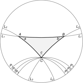
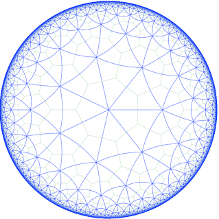
Because of the fundamental difficulties in representing spaces of constant negative curvature as subsets of Euclidean spaces, there are not one but many equivalent models of hyperbolic spaces. Each model emphasizes different aspects of hyperbolic geometry, but no model simultaneously represents all of its properties. In special relativity, for example, the hyperboloid model is commonly used, where the hyperbolic space is represented by a hyperboloid. Its two different projections to disks orthogonal to the main axis of the hyperboloid yield the Klein and Poincaré unit disk models. In the latter model, the whole infinite hyperbolic plane , i.e., the two-dimensional hyperbolic space of constant curvature , is represented by the interior of the Euclidean disk of radius , see Fig. 1. The boundary of the disk, i.e., the circle , is not a part of the hyperbolic plane, but represents its infinitely remote points, called boundary at infinity . Any symmetry transformation on translates to a symmetry on , and vice versa, a cornerstone of the anti-de Sitter space/conformal field theory correspondence Maldacena (1999); Gubser et al. (1998); Witten (1998), where quantum gravity on an anti-de Sitter space is equivalent to a quantum field theory without gravity on the conformal boundary of the space. Hyperbolic geodesic lines in the Poincaré model, i.e., shortest paths between two points at the boundary, are disk diameters and arcs of Euclidean circles intersecting the boundary perpendicularly. The model is conformal, meaning that Euclidean angles between hyperbolic lines in the model are equal to their hyperbolic values, which is not true with respect to distances or areas. Euclidean and hyperbolic distances, and , from the disk center, or the origin of the hyperbolic plane, are related by
| (1) |
The model is generalizable for any dimension , in which case is represented by the interior of the unit ball whose boundary is the boundary at infinity . The model is related via the stereographic projection to another popular model—the upper half-space model—where is represented by a “half” of span by vectors with . The boundary at infinity in this case is the hyperplane instead of . Essentially any -dimensional space with a -dimensional boundary can be equipped with a hyperbolic metric structure, with the ’s boundary playing the role of the boundary at infinity .
Given the abundance of hyperbolic space representations, we are free to choose any of those, e.g., the one most convenient for our purposes. Unless mentioned otherwise, we use the native representation in the rest of the paper. In this representation, all distance variables have their true hyperbolic values. In polar coordinates, for example, the radial coordinate of a point is equal to its hyperbolic distance from the origin. That is, instead of (1), we have
| (2) |
A key property of hyperbolic spaces is that they expand faster than Euclidean spaces. Specifically, while Euclidean spaces expand polynomially, hyperbolic spaces expand exponentially. In the two-dimensional hyperbolic space of constant curvature , , for example, the length of the circle and the area of the disk of hyperbolic radius are
| (3) | |||||
| (4) |
both growing as with . The hyperbolic distance between two points at polar coordinates and is given by the hyperbolic law of cosines
| (5) |
where is the angle between the points. Equations (3-5) converge to their familiar Euclidean analogs at . For sufficiently large , , and , the hyperbolic distance is closely approximated by
| (6) |
That is, the distance between two points is approximately the sum of their radial coordinates, minus some -dependent correction, which goes to zero at .
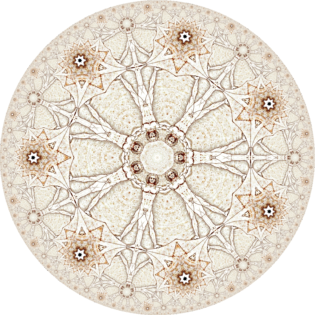
Hyperbolic spaces are similar to trees. In a -ary tree (a tree with branching factor ), the analogies of the circle length or disk area are the number of nodes at distance exactly or not more than hops from the root. These numbers are and , both growing as with . We thus see that the metric structures of and -ary trees are the same if : in both cases circle lengths and disk areas grow as . In other words, from the purely metric perspective, and -ary trees are equivalent. Informally, trees can therefore be thought of as “discrete hyperbolic spaces.” Formally, trees, even infinite ones, allow nearly isometric embeddings into hyperbolic spaces. For example, any tessellation of the hyperbolic plane (see Fig. 1) naturally defines isometric embeddings for a class of trees formed by certain subsets of polygon sides. For comparison, trees do not generally embed into Euclidean spaces. Informally, trees need an exponential amount of space for branching, and only hyperbolic geometry has it.
| Property | Euclidean | Spherical | Hyperbolic |
| Curvature | |||
| Parallel lines | |||
| Triangles are | normal | thick | thin |
| Shape of triangles | |||
| Sum of angles | |||
| Circle length | |||
| Disk area |
Table 1 collects these and other characteristic properties of hyperbolic geometry and juxtaposes them against the corresponding properties of Euclidean and spherical geometries.
III Topological heterogeneity versus geometrical hyperbolicity
In this section we make high-level observations suggesting the existence of intrinsic connections between hyperbolic geometry and the topology of complex networks.
Complex networks connect distinguishable, heterogeneous elements abstracted as nodes. Understood broadly, this heterogeneity implies that there is at least some taxonomy of elements, meaning that all nodes can be somehow classified. In most general settings, this classification implies that nodes can be split in large groups consisting of smaller subgroups, which in turn consist of even smaller subsubgroups, and so on. The relationships between such groups and subgroups can be approximated by tree-like structures, sometimes called dendrograms, which represent hidden hierarchies in networks Clauset et al. (2008). But as discussed in the previous section, the metric structures of trees and hyperbolic spaces are the same. We emphasize that we do not assume that the node classification hierarchy among a particular dimension is strictly a tree, but that it is approximately a tree. As soon as it is at least approximately a tree, it is negatively curved Gromov (2007). This argument obviously applies only to a snapshot of a network taken at some moment of time. A logical question is how these taxonomies emerge. Clearly, when a network begins to form, the node classification is degenerate, but as more and more nodes join the network and evolve in it, they tend to diversify and specialize, thus deepening their classification hierarchy. The distance between nodes in such hierarchies is then a rough approximation of node similarity, and the more similar a pair of nodes, the more likely they are connected.
We consider several examples suggesting that these general observations apply to different real networks. Social networks form the most straightforward class of examples, where network community structures Girvan and Newman (2002); Boguñá et al. (2004a) represent hidden hierarchies Watts et al. (2002). More concretely, in paper citation networks, the underlying geometries can approximately be the relationships between scientific subject categories, and the closer the subjects of two papers, the more similar they are, and the more likely they cite each other Redner (1998); Börner et al. (2004). Classifications of web pages (or more specifically, of the Wikipedia pages Muchnik et al. (2007); Crandall et al. (2008)) also show the same effect: the more similar a pair of web pages, the more likely that there is a hyperlink between them Menczer (2002). In biology, the distance between two species on the phylogenetic tree is a widely used measure of similarity between the species Nei and Kumar (2000). Note that this example emphasizes both the existing taxonomy of elements and their evolution. The evolution of the Internet is yet another paradigmatic example. In the beginning, there were only a couple of computers connected to each other, but then the network grew Leiner et al. (1997) splitting into a collection of independently administered networks, called autonomous systems (ASs), whose number and diversity have been growing fast Dhamdhere and Dovrolis (2008). Currently, ASs can be classified based on their geographic position and coverage, size, number and type of customers, business role, and many other factors Dhamdhere and Dovrolis (2008); Dimitropoulos et al. (2006).
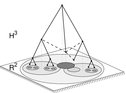
The general observation that the metric structure of node similarity distances is hyperbolic follows from the mathematical fact illustrated in Fig. 2. We assume there that a point in represents an abstract node attribute or characteristic, while a Euclidean disk in represents a collection of all the attributes for a given node in the network. The network itself is not shown. Instead we visualize a hidden hierarchy arising from the overlapping disks. The more two disks overlap, the more similar the sets of characteristics of the two corresponding nodes, that is, the more similar the nodes themselves. But the mapping between disks and nodes in in Fig. 2 is such that the more the two disks overlap, the hyperbolically closer are the corresponding two nodes. Formally, if the ratio of the disks’ radii is bounded by a constant , , and the Euclidean distance between their centers is bounded by , then the hyperbolic distance between the corresponding nodes in is bounded by some constant , which depends only on , and not on the disk radii or center locations Gromov (2007). The converse is also true. Therefore, the distances between nodes based on similarity of their attributes can be mapped to distances in a hyperbolic space, assuming that node attributes possess some metric structure ( in the above example) in the first place.
IV Hyperbolic geometry yields heterogeneous topology
We now put the intuitive considerations in the previous section to qualitative grounds. We want to see what network topologies emerge in the simplest possible settings involving hyperbolic geometry.
IV.1 Uniform node density at curvature
Since the one-dimensional hyperbolic space does not exist, the simplest hyperbolic space is the hyperbolic plane discussed in Section II. The simplest way to place nodes on the hyperbolic plane is to distribute them uniformly over a disk of radius , where abstracts the depth of the hidden tree-like hierarchy. We will see below that is a growing function of , reflecting the intuition in Section III that the network hierarchy deepens with network growth. The hyperbolically uniform node density implies that we assign the angular coordinates to nodes with the uniform density , while according to Eqs. (3,4) with , the density for the radial coordinate is exponential
| (7) |
To form a network, we need to connect each pair of nodes with some probability, which can depend only on hyperbolic distances between nodes. The simplest connection probability function is
| (8) |
where is the Heaviside step function. We will justify and relax this choice in Section VI. This connection probability means that we connect a pair of nodes by a link only if the hyperbolic distance (5) between them is .
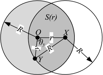
The network is now formed, and we can analyze its topological properties. We are first interested in the most basic one, the degree distribution , to compute which we have to calculate the average degree of nodes located at distance from the origin. Since the node density is uniform, is proportional to the area of the intersection of the two disks shown in Fig. 3. Specifically, with node density . The area element in polar coordinates is , cf. Eqs. (3,4) with . Therefore, the intersection area is given by the following integration illustrated in Fig. 3
| (9) | |||||
where is given by the hyperbolic law of cosines (5) for the triangle in Fig. 3
| (10) |
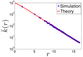
Solving the last equation for and substituting the result into (9) yields the exact expression for and consequently for the average degree
| (11) | |||||
which perfectly matches simulations in Fig. 4. For large this terse exact expression is closely approximated by
| (12) |
where the last approximation holds for large .
The average degree in the network is then
| (13) |
from which we conclude that if we want to generate an -node network with a target average degree we have to select the disk radius . We see that scales with as , i.e., the same way as the depth of a balanced tree with its size. We also observe that by fixing
| (14) |
we gain control over the average degree in a network via parameter , using which we rewrite (12) as
| (15) |
To finish computing the degree distribution we treat the radial coordinate as a hidden variable in the terminology of Boguñá and Pastor-Satorras (2003), yielding , where the propagator is the conditional probability that a node with hidden variable has degree . For sparse networks this propagator is Poissonian Boguñá and Pastor-Satorras (2003), , using which we finally obtain
| (16) |
That is, the node degree distribution is a power law.
This result is remarkable as we have done nothing to enforce this power law. Network heterogeneity has naturally emerged as a direct consequence of the basic properties of hyperbolic geometry underlying the network. Indeed, the observed power law is a combination of two exponentials Newman (2005), node density in (7) and average degree in (15), both reflecting the exponential expansion of space in hyperbolic geometry discussed in Section II.
IV.2 Quasi-uniform node density at arbitrary negative curvature
We next relax two constraints in the model. The first constraint is that the node density is exactly uniform. We let it be quasi-uniform,
| (17) |
that is, exponential with exponent . In terms of the analogy with trees in Sections II,III, this relaxation is equivalent to assuming that the hidden tree-like hierarchy has the average branching factor . Second, we let the curvature of the hyperbolic space be any with . The node density is exactly uniform now only if .
The exact expression for the average degree of nodes at distance from the origin is the same as before,
but we cannot compute it exactly to yield an answer analogous to (11). However, approximations are easy. The main approximation deals with the angle in Fig. 3. Instead of (10), we now have according to (5)
| (19) |
which for large , , and yields . Substituting this in the integral for (IV.2), using there the approximate expression for in (17), and introducing notation , we obtain
| (20) | |||||
| (21) |
The average degree in the whole network is now
| (22) |
and its limit at is well defined,
| (23) |
If , we can neglect the second term in (22), leading to
| (24) |
That is, the condition controlling the average degree in the network changes from (14) to
| (25) |
where the control parameter . This control is the less accurate, the closer the to . Indeed, as approaches , the relative contribution to the total average degree coming from the second term in (22) increases. In particular, if , then is undefined, meaning that can no longer be . If instead of solving Eq. (23) to find radius for given and , we fix according to (25) with some , then similar to Krapivsky and Redner (2005), the average degree in (23) will grow polylogarithmically with the networks size,
| (26) |
If we neglect the second terms in (22,20) at , then using (25), we rewrite (20) as
| (27) |
That is, somewhat surprisingly, the scaling of the average degree with radius does not depend on the exponent of the node density. Proceeding as in Section IV.1, the degree distribution for is then
| (28) |
For arbitrary values of the degree distribution scales as
| (29) |
We observe that the node density exponent and the space curvature affect the heterogeneity of network topology, parameterized by , only via their ratio . This result is intuitively expected in view of the analogy to trees discussed in Sections II,III, since a tree with branching factor is metrically equivalent to the two-dimensional hyperbolic space with curvature . In other words, the branching factor of a tree and the curvature of a hyperbolic space are two different measures of the same metric property—how fast the space expands. Result (29) states then that the topology of networks built on top of these metric structures depends only on the appropriate normalization, , between the two measures.
The model described so far has thus only two parameters, and , controlling the degree distribution shape and average degree. The model produces scale-free networks with any power-law degree distribution exponent . The uniform node density in the hyperbolic space corresponds to , and results in , i.e., the same exponent as in the original preferential attachment model Barabási and Albert (1999). Since , the average degree of nodes at distance from the origin (27), and the total average degree in the network are
| (30) | |||||
| (31) |
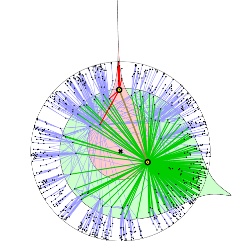
A sample network is visualized in Fig. 5.
V Heterogeneous topology implies hyperbolic geometry
In the previous section, we have shown that networks constructed over hyperbolic spaces naturally possess heterogeneous scale-free degree distributions. In this section we show the converse. Assuming that a scale-free network has some metric structure underneath, we show that metric distances can be naturally rescaled such that the resulting metric space is hyperbolic.
To accomplish this task we use the model from Serrano et al. (2008) where the underlying metric structure is abstracted by the simplest possible compact metric space, circle . This model generates networks as follows. First, nodes are placed, uniformly distributed, on a circle of radius so that the node density on the circle is fixed to . Then each node is assigned its expected degree, which is a random variable drawn from the continuous power-law distribution
| (32) |
where is the target degree distribution exponent, and is the minimum expected degree. Finally, each node pair with expected degrees and angular coordinates located at distance over the circle () is connected with probability , which can be any integrable function of
| (33) |
where is the parameter controlling the average degree in the network. This form of the argument of the connection probability function is the only requirement to ensure that the average degree of nodes with expected degree in the constructed network is indeed proportional to , specifically , where is the average degree in the network as before, and
| (34) |
Due to this proportionality, the degree distribution in the network is indeed power-law distributed with exponent .
To see that condition (33) ensures , set without loss of generality, let , and observe that Boguñá and Pastor-Satorras (2003)
| (35) | |||||
Since
| (36) |
we conclude that , and confirm that controls the average degree in the network. We also note that is a dumb parameter, which can be set to leading to .
We now establish the equivalence between this model and the model described in the previous section. To do so, we need to find a change of variables from , expected degree of a node, to , its radial coordinate on a disk of radius , such that if variable is power-law distributed according to (32), then after this -to- change of variables, variable is exponentially distributed according to (17). The change of variables that accomplishes this task is
| (37) |
where is a parameter defining in (17) after this change of variables. The resulting value of is , which is the same relationship among , , and as in (29). In other words, after the -to- mapping above, the nodes get distributed on the disk as in the model, suggesting that parameter is actually the space curvature.
To check if it is indeed the case, and if the two models are indeed equivalent, we have to verify that the pairs of nodes connected or disconnected in the model with expected degree mapped to radial coordinate correspond to, respectively, connected or disconnected nodes in the native model. That is, we have to demonstrate that the connection probabilities in the two models are consistent, . To show this we first fix the disk radius to its value in the model (25), and then observe that if we set
| (38) |
then the change of variables (37) maps the argument of the connection probability in the model (33) to
| (39) |
where is equal to the second approximation of the hyperbolic distance in (6). Therefore, the connection probability in the model is approximately equal to the connection probability in the model. In particular, the step function connection probability (8) in the model corresponds to
| (40) |
in the model. The integral of this connection probability is obviously , so that the vs relationship (36) in the model becomes , which is consistent with the condition (38) given the .vs. relationship in the model (31). As the final consistency check, we observe that the substitution of the -to- mapping into the proportionality in the model yields (30) in the model. That is, the average degrees of nodes with radial coordinate in the and models are the same.
The two models are thus equivalent, and with the appropriate choice of parameters, generate statistically the same ensembles of networks, which one can confirm in simulations. In this section the network metric structure has been modeled the simplest way, by circle , which by no means is the only possibility for the hyperbolic space boundary , see Section II. Therefore, the established equivalence between the and models suggests that as soon as a heterogeneous network has some metric structure induced by distances on , this metric structure can be rescaled by node degrees to become hyperbolic, using appropriate modifications of (33,39). The heterogeneous degree distribution effectively adds an additional dimension to (the radial dimension in the case), such that the resulting space ( in the considered case) is hyperbolic, a mechanism conceptually similar to how time in special relativity, or gravity in Maldacena (1999); Gubser et al. (1998); Witten (1998) makes the higher-dimensional (time)space hyperbolic. In other words, hyperbolic geometry naturally emerges from network heterogeneity, the same way as network heterogeneity emerges from hyperbolic geometry in the previous section.
VI Hyperbolic geometry versus statistical mechanics
In this section we relax the final constraint in the model that the connection probability is a step function, and provide a statistical mechanics interpretation of the resulting network ensemble.
Since can be any integrable function in the version of the model, can be any function in the version. Given this freedom, we consider the following family of connection probability functions,
| (41) |
parameterized by . The function is integrable for any ,
| (42) |
However, we will not restrict , and will also consider .
The main motivation for the connection probability choice (41) is that it casts the ensemble of graphs in the model to exponential random graphs Dorogovtsev et al. (2003); Park and Newman (2004); Garlaschelli and Loffredo (2009); Anand and Bianconi (2009); Bianconi (2009). Exponential random graphs are maximally random graphs subjected to specific constraints, each constraint associated with an auxiliary field or Lagrangian multiplier in the standard entropy maximization approach, commonly used in statistical mechanics. Each graph in the ensemble has probability weight , where is the graph Hamiltonian, and is the partition function. For example, the ensemble of graphs in the configuration model, i.e., graphs with a given degree sequence , is defined by Hamiltonian , where are the auxiliary fields coupled to nodes , and is ’s adjacency matrix. A natural generalization of this ensemble Park and Newman (2004) is given by the Hamiltonian in which the auxiliary fields are coupled not to nodes but to links . The partition function is then
| (43) |
and the probability of link existence between nodes and is given by Park and Newman (2004)
| (44) |
The connection probability (41) thus interprets the auxiliary fields in this ensemble as a linear function of hyperbolic distances between nodes in the ensemble of graphs generated by our model,
| (45) |
which makes the two ensembles identical.
The connection probability (41) is nothing but the Fermi-Dirac distribution. It appears because we allow only one link between a pair of nodes. If we allowed multiple links, or if we considered weighted networks, the resulting link statistics would be Bose-Einstein Park and Newman (2004); Garlaschelli and Loffredo (2009). Hyperbolic distances in (41) can now be interpreted as energies of fermionic links, whereas hyperbolic disk radius is the chemical potential, is the Boltzmann constant, and is the inverse temperature. The ensemble is grand canonical with the number of particles or links fixed on average. The standard definition of the chemical potential is then
| (46) |
where is the degeneracy of energy level . In our case, is the probability that two nodes are located at distance from each other. We can compute this probability to yield
| (47) |
where are some constants, and . Substituting this in definition (46), using there, and keeping the leading terms, we get
| (48) |
where is another constant which we determine in the next section. If , we neglect the second term above, and observe that the standard definition of the chemical potential in statistical mechanics (46) yields the same result as (25), obtained using purely geometric arguments. The same observation applies for the parameter that we get from (48): it is the same as in (36) with and in (34), or as in (31) if temperature , so that .
At the system is in the ground, most degenerate state, and all links occupy the lowest energy levels until all of them are filled. In this ground state, Fermi distribution (41) converges to the step function (8), which a posteriori justifies our choice there. At higher temperatures the fermionic particles start populating higher energy states, and at we have a phase transition caused by the divergence of leading to a discontinuity of the partition function (43). This discontinuity is due to the discontinuity of the chemical potential . We see from (48,42) that diverges as at . If , then the second term in (48) is the leading term, and instead of (25) we have
| (49) |
so that at , the chemical potential diverges as . We investigate what effect this phase transition has on network topology in the next two sections.
VII Degree distribution at non-zero temperature
VII.1
Since the connection probability in (41) is integrable in this cold regime, we immediately conclude that the degree distribution is the same power law as at the zero temperature, while the average degree is (36) with in (42). In view of the equivalence between the and models established in Section V, the power-law exponent is related to the model parameters and via , as at . The chemical potential is with (25,38).
VII.2
In this hot regime, the connection probability diverges, and we have to renormalize its integral . Specifically, instead of integrating to infinity as in (35), we have to explicitly cut off the integration at the maximum value of . The exact value of with in (41) is , where is the Gauss hypergeometric function. The leading term of this product for large and is , substituting which into the expression for the average degree in the model (35) we get
| (50) | |||||
| (51) | |||||
| (52) |
where is the input value of the -parameter in the model, i.e., the distribution of the hidden variable is . We introduce a new notation for this parameter to differentiate it from the value of power-law exponent in generated networks, which is different from in this hot regime. Indeed, since the average degree of nodes with hidden variable is no longer proportional to but to (50), the degree distribution in the modeled networks is
| (53) |
The mapping to the model is achieved via the same change of variables (37), and by requiring that . Performing this change of variables, and noticing that , we obtain the following key relationships in the model:
| (54) | |||||
| (55) | |||||
| (56) | |||||
| (57) |
The last two equations fill in the coefficient in the expression for the chemical potential (49).
Finally, we note that in the hot regime the admissible range of input parameters controlling the degree distribution exponent is () or (), both yielding .
VIII Clustering as a function of temperature
VIII.1
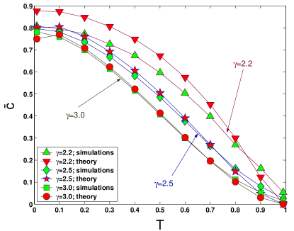
In the cold regime, the average clustering is a decreasing function of temperature, see Fig. 6. Clustering is maximized at , and it gradually, almost linearly, decreases to zero at the phase transition point .
Unfortunately, cannot be computed analytically, but some estimates for specific values of are possible. The average clustering of nodes with expected degree in the model is the probability that two nodes with expected degrees and angular coordinates and , both connected to node with (we set without loss of generality), are connected to each other. Introducing notations for the three rescaled distances , , and , where , this probability is given by Boguñá and Pastor-Satorras (2003)
| (58) | |||||
Changing the integration variables from and to and in the second integral, extending the integration limits to infinity, and using the expression for the average degree in the model (35), yield
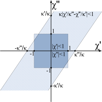
At , , while . Therefore, the inner integral in the last expression reduces to the area of the intersection of the square defined in the coordinates by , and the stripe , see Fig. 7. For small , the stripe is so wide for almost any combination of that it fully contains the square, whose area is , so that proving that clustering is maximized at the zero temperature. Recall that clustering cannot be for all node degrees because of structural constraints Serrano and Boguñá (2005). For arbitrary values of , the exact expression for the intersection area involves cumbersome combinatorial conditions for the mutual relationship among , , and , which make taking the outer integral in (VIII.1) problematic. However one can check that for large , , where is a decreasing function of .
For any other values of , the inner integral in (VIII.1) can be taken by residues, but the number of poles depends on . At , for example, the inner integral is , so that for we have the exact expression for
| (60) | |||||
and , while for large . For other values of , one can show that , where is also a decreasing function of .
VIII.2
In the hot regime, temperature has no effect on clustering, which is always zero for large networks. This effect can be confirmed in simulations, and seen analytically. Indeed, observe that in view of (50-52), the -to- change of variables, turning (58) into (VIII.1), now yields the pre-factor in the latter equal to instead of . This new pre-factor is obviously zero in the thermodynamic limit.
IX Connection to the configuration model and classical random graphs
Since clustering does not depend on temperature in the hot regime, while the power-law exponent (54) depends on temperature via the ratio , we can let and , but fix their ratio to be a new parameter . With this parameter the key equations (54,56,57) in the model become
| (61) |
But since curvature , the last -dependent term in the expression for the hyperbolic distance (6) is zero. Since this term reflects the presence of the metric structure in the network, its disappearance effectively destroys this structure. More formally, the network metric structure becomes degenerate, because the hyperbolic distance between a pair of nodes and reduces to the sum of their radial coordinates, , as a result of which the auxiliary fields (45) decouple, , where . Therefore, the probability of the existence of link in (44) depends now only on the product of ’s expected degrees given by (55), , so that the network ensemble becomes the ensemble of networks in the configuration model, i.e., the ensemble of graphs with given expected degrees Chung and Lu (2002).
Alternatively, we can keep both and finite while heating the networks up by increasing . In this case, Eqs. (54-57) converge to , , , and , while the Fermi-Dirac connection probability (41) becomes uniform . That is, all nodes get uniformly distributed on the boundary at infinity , and each pair of nodes is connected with the same probability , independent of their distances. We note that the distance between two points with angular coordinates is Buyalo and Schroeder (2007)—compare with (6) in and with in the other limiting case, the configuration model. The limiting degree distribution is Poissonian (), and the network ensemble converges to the ensemble of classical random graphs with a given average degree Erdős and Rényi (1959). The network in this case loses not only its metric structure, but also its hierarchical heterogeneous organization.
| Property | Cold regime | Hot regime | ||
|---|---|---|---|---|
| (36) | (38) | (51) | (56) | |
| (32) | (29) | (53) | (54) | |
| (Fig. 6) | ||||
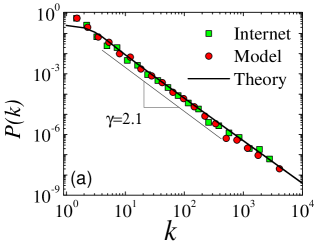
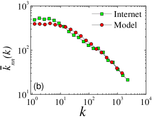
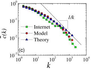
Here, we finish the description and analysis of our geometric model of complex networks. To summarize, the model can produce scale-free networks with any average degree , power-law exponent , and average clustering , controlled, respectively, by parameters and in the and formulations of the model, see Table 2. In Fig. 8 we observe a good match between the basic topological properties of the real Internet and a synthetic network generated by the model with an appropriate choice of parameters in the cold regime. In the hot regime the model subsumes the standard configuration model and classical random graphs as two different limiting cases with degenerate geometric structures.
X Efficiency of greedy navigation in modeled networks
In this section we shift our attention from the analysis of the structure of complex networks in our model to the analysis of their function. Specifically, we are interested in their navigation efficiency.
One important function that many real networks perform is to transport information or other media. Examples include the Internet, brain, or signaling, regulatory, and metabolic networks. The information transport in these networks is not akin to diffusion. Instead information must be delivered to specific destinations, such as specific hosts in the Internet, neuron groups in the brain, or genes and proteins in regulatory networks. In the latter case, for example, the network reacts to an increased concentration of some sugar by expressing not all but very specific proteins, the ones responsible for digesting this sugar. At the same time the nodes in the network are not aware of the global network structure, so that the questions we face are if paths to specific destinations in the network can be found without such global topology knowledge, and how optimal these paths can be.
The salient feature of our model is that it allows one to study the efficiency of such path finding without global knowledge, because our networks have underlying geometry which enables greedy forwarding (GF). Since each node in the network has its address, i.e., coordinates in the underlying hyperbolic space, a node can compute the distances between each of its neighbors in the network, and the destination whose coordinates are written in the information packet, or encoded in the signal. GF then accounts to forwarding the information to the node’s neighbor closest to the destination in the hyperbolic space. Since each node knows only its own address, the addresses of its neighbors, and the destination address of the packet, no node has any global knowledge of the network structure.
We report simulation results for two forms of GF, original GF (OGF) and modified GF (MGF). The OGF algorithm drops the packet if the current node is a local minimum, meaning that it does not have any neighbor closer to the destination than itself. The MGF algorithm excludes the current node from any distance comparisons, and finds the neighbor closest to the destination. The packet is dropped only if this neighbor is the same as the packet’s previously visited node.
These GF processes can be very inefficient. They can often get stuck at local minima, or even if they succeed reaching the destination, they can travel along paths much longer than the optimal shortest paths available in the network. Furthermore, even if they are efficient in static networks, their efficiencies can quickly deteriorate in the presence of network topology dynamics, e.g., they can be vulnerable with respect to network damage.
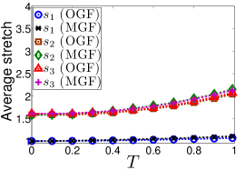
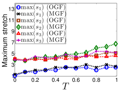
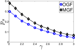
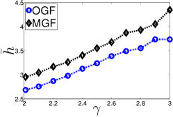
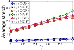
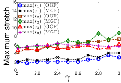
To estimate the GF efficiency in static networks, we compute the following metrics: (i) the percentage of successful paths, , which is the proportion of paths that reach their destinations; (ii) the average hop-length of successful paths; and (iii) the average and maximum stretch of successful paths. We consider three types of stretch. The first stretch is the standard hop stretch defined as the ratio between the hop-lengths of greedy paths and the corresponding shortest paths in the graph. We denote its average and maximum by and . The optimal paths have stretch equal to . The other two stretches are hyperbolic. They measure the deviation of the hyperbolic length, traveled by a packet along either the greedy or shortest path, from the hyperbolic distance between the source and destination. Formally, let be a source-destination pair and let be the greedy or shortest path between and , and its hop length. Further, let , be the hyperbolic distance between and . The hyperbolic stretch is the ratio , where is the hyperbolic distance between and . For greedy paths, we denote the average and maximum of this stretch by and ; for shortest paths those are denotes by and . The lower these two stretches, the closer the greedy and shortest paths stay to the hyperbolic geodesics, and the more congruent we say the network topology is with the underlying geometry.
We first focus on static networks, where the network topology does not change, and then emulate the network topology dynamics by randomly removing one or more links from the topology. For each generated network instance, we extract the giant connected component (GCC), and perform GF between random source-destination pairs belonging to the GCC. All the metrics converge after approximately source-destination pairs, but we evaluate an order of magnitude more combinations for more reliable results. The network size is , and the average degree is in all the experiments, while temperature only in the following two subsections.
X.1 Static networks
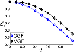
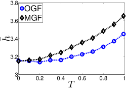
Figure 9 shows the results for static networks, averaged, for each , over five network instances. We see that the success ratio increases and path length and all the stretches decrease as we decrease to . Remarkably, for , e.g., equal to the observed in the Internet, OGF and MGF yield and , with the OGF’s maximum stretch of , meaning that all greedy paths are shortest paths. Interestingly, the hyperbolic stretch of shortest paths ( and ) is slightly worse (larger) than of greedy paths ( and ), which allows us to informally say that for small ’s, greedy paths are “shorter than shortest” as they are shortest hop-wise, but GF tends to select among many shortest paths those of least hyperbolic stretch.
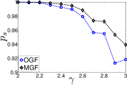
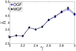
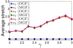
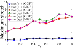
In summary, GF is exceptionally efficient in static networks, especially for the small ’s observed in the vast majority of complex networks, including the Internet. The GF efficiency is maximized in this case, and the two algorithms exhibit almost the best possible performance, with reachability reaching almost , and all greedy paths being optimal (shortest).
X.2 Dynamic networks
We next look at the GF performance in dynamic networks with link failures. For each , we randomly select a network instance from above and remove one or more random links in it. We consider the following two link-failure scenarios. In Scenario 1 we remove a percentage , ranging from to , of all links in the network, compute the new GCC, and for all source-destination pairs remaining in it, we recompute the new success ratio , and the average and maximum stretch and . In Scenario 2 we provide a finer-grain view focusing on paths that used a removed link. We remove one link from the network, compute the new GCC, and for the source-destination pairs that are still in it, we find the percentage of successful paths, only among those previously successful paths that traversed the removed link. For these still-successful paths, we also compute the new average and maximum stretch and . We then repeat the procedure for random links, and report the average values for and , and the maximum value for .
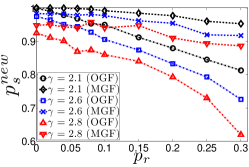
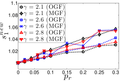
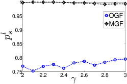
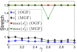
Figure 10 presents the results. We see that for small ’s, the success ratio remains remarkably high, for all meaningful values of . For example, MGF on networks with and , yields . The simultaneous failure of of the links in a network such as the Internet is a rare catastrophe, but even after such a catastrophe the success ratio in our synthetic networks is above . The average stretch slightly increases as we increase , but remains quite low. We do not show to avoid clutter. For , . The percentage of MGF paths that used a removed link and that found a by-pass after its removal is also remarkably close to for small ’s. The average stretch in Scenario 2 also remains low, below , and the maximum stretch never exceeds .
In summary, GF is not only efficient in static networks, but its efficiency is also robust in the presence of network topology dynamics. In particular, for small ’s matching those found in real networks such as the Internet, GF maintains remarkably high reachability and low stretch, even after catastrophic damages to the network.
X.3 Role of clustering
Next we fix , and investigate the GF performance as a function of temperature in Fig. 11. The picture is qualitatively similar to Fig. 9. The GF efficiency is the better, the smaller is the temperature, i.e., the stronger the clustering, see Fig. 6. At zero temperature where clustering is maximized, GF demonstrates the best possible performance, as discussed in Section X.1.
X.4 Random graphs
Finally, we look at the GF performance in the configuration model and classical random graphs, which are two different degenerate cases with zero clustering in our geometric network ensemble, see Section IX.
To test the configuration model, we fix , so that , compute distances between nodes according to , and show the results in Fig. 12. We observe that the GF efficiency is poor in this case. The success ratio never exceeds , and drops to below for large ’s. This poor performance is expected. Indeed, since , GF reduces to following the node degree gradient. Each node just forwards the packet to its highest-degree neighbor since this neighbor has the smallest radial coordinate , thus minimizing the distance to the destination. If during this process the packet reaches the highest-degree hub in the network core, without visiting a node directly connected to the destination, then it gets stuck at this hub, because no angular coordinates instructing in what direction to exit the core are any longer available—a problem, which does not admit a simple and efficient solution Adamic et al. (2001).
To test classical random graphs, we assign to nodes their angular coordinates uniformly distributed on , connect each node pair with the same probability , and compute distances according to . Greedy forwarding is extremely inefficient in this case. The OGF and MGF average success ratios are and .
In summary, the hierarchical organization (heterogeneous degree distribution) and metric structure (strong clustering) in the network are both critically important for network navigability.
X.5 Why hierarchical structure and strong clustering ensure efficient navigation
We have seen that more heterogeneous networks (smaller ) with stronger clustering (smaller ) are more navigable. Here, we explain why it is the case.
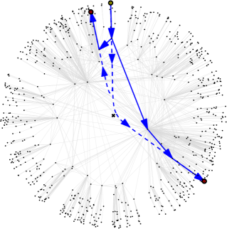
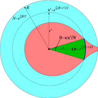
We first recall that the congruency, measured by the hyperbolic stretch, between the network topology and hyperbolic geometry is the stronger, the smaller are the and , see Figs. 9,11. To visualize this effect, we draw in Fig. 13(a) a couple of GF paths and their corresponding hyperbolic geodesics. We see that the lengths of the latter are indeed dominated by the sums of the radial coordinates of the source and destination, minus some -dependent corrections (6). This domination of the radial direction shapes the following hierarchical path pattern of the hyperbolic geodesics, as well as of the corresponding GF paths: (i) zoom-out from the network periphery to the core, moving to increasingly higher-degree nodes, that is, nodes covering increasingly wider areas by their connections, see Fig. 5; (ii) turn in the core to the direction of the destination; and finally (iii) zoom-in onto it, moving to lower-degree nodes. This path pattern is exactly the pattern of hierarchical paths in Trusina et al. (2004). A path is called hierarchical in Trusina et al. (2004) if it consists of two segments: first, a segment of nodes with increasing degrees, and then a segment of nodes with decreasing degrees. As shown in Trusina et al. (2004) (see Fig. 2(a) there), the percentage of shortest paths that are also hierarchical approaches with . Remarkably, this hieratical path pattern also characterizes the policy-compliant paths followed by information packets in the Internet Gao (2001); Dimitropoulos et al. (2007). Since the GF paths, also the shortest paths in the network, follow the shortest geodesic paths in the hyperbolic space, the resulting hyperbolic stretch is small. Thanks to strong clustering, the network has many partially disjoint paths between the same source and destination, which all follow the same hierarchical pattern. Therefore, even if some paths are damaged by link failures, other congruent paths remain, and GF can still find them using the same hyperbolic geodesic direction, which explains the high robustness of network navigability with respect to network damage. As clustering weakens, not only the path diversity in the network decreases, but also the network metric structure deteriorates, since the edge existence probability (41) depends less and less on the hyperbolic distance between nodes. In the extreme case of classical random graphs, for example, the connection probability does not depend on this distance at all. As a result, the congruency between network topology and underlying geometry evaporates.
Heterogeneity is another key element responsible for high navigability. This heterogeneity is nothing but a reflection of the hierarchical, tree-like structure of the underlying hyperbolic space. Indeed, its hierarchical structure manifests itself in the hierarchy of node degrees, and in the degree-dependent amount of space that nodes cover by their connections. As Fig. 5 shows, nodes of higher degrees, closer to the top of the hierarchy, cover wider areas with their connections. To quantify, at the angular sector that nodes with expected degree cover by their connections to nodes with expected degree , see Fig. 13(b), is . This degree-dependent hierarchy of space coverage makes the hierarchical zooming-out/zooming-in path pattern possible and successful.
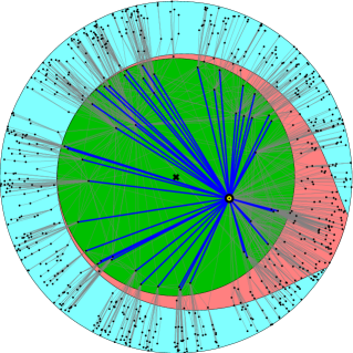
Finally, the stronger the heterogeneity, the more bridges are in the network, where by bridges we mean nodes that connect to all nodes with expected degrees exceeding a certain threshold, an example is shown in Fig. 13(c). This threshold is given by the equation , yielding that a node with expected degree is connected to all nodes with expected degrees . However such -degree nodes may not exist in the network, as the required may exceed the maximum expected degree Boguñá et al. (2004b). Requiring leads to . That is, only such -degree nodes are expected to be bridges. The equation for the expected bridge existence is then , yielding . That is, bridges exist in any sufficiently large network with —the smaller the is, the more bridges and the longer they are—while networks with have no bridges. The role of bridges in the network core is straightforward: as soon as GF reaches a bridge, it can cross the entire network, in any direction, at one hop Boguñá and Krioukov (2009). Without bridges, GF is doomed to wander along the network periphery, endangered by getting lost there at any hop. The GF success ratio in networks with deteriorates to zero in the thermodynamic limit Boguñá et al. (2009).
XI Conclusion
We have developed a framework to study the structure and function of complex networks in purely geometric terms. In this framework, two common properties of complex network topologies, strong heterogeneity and clustering, turn out to be simple reflections of the basic properties of an underlying hyperbolic geometry. Heterogeneity, measured in terms of the power-law degree distribution exponent, is a function of the negative curvature of the hyperbolic space, while clustering reflects its metric property.
Conversely, a heterogeneous network with a metric structure has an effective hyperbolic geometry underneath. This finding sheds light on self-similarity in complex networks Serrano et al. (2008). The network renormalization procedure considered in Serrano et al. (2008)—throwing out nodes of degrees exceeding a certain threshold—is equivalent to contracting the radius of the hyperbolic disk where all nodes reside. This contraction is a homothety along the radial direction, which is a symmetry transformation of the hyperbolic space, and self-similarity of hyperbolic spaces with respect to such homothetic transformations has been formally defined and studied Buyalo and Schroeder (2007). Self-similarity of complex networks thus appears as a reflection of self-similarity of hyperbolic geometry, or as the invariance with respect to symmetry transformations in the underlying space.
The developed framework establishes a clear connection between statistical mechanics and hyperbolic geometry of complex networks. The collection of edges in a network, for example, can be treated as a system of non-interacting fermions whose energies are the hyperbolic distances between nodes. This geometric interpretation may lead to further developments applying the standard tools of statistical mechanics to network analysis.
The network ensemble in our framework subsumes the standard configuration model and classical random graphs as two limiting cases with degenerate geometric structures. The hyperbolic distance between two nodes (6) delicately combines their radial and angular coordinates. In the configuration model, the distance degenerates to the sum of radial coordinates only, destroying the network metric structure. In classical random graphs, on the contrary, there is no radial distance dependence. The connection probability between nodes does not depend on any distances at all. As a result, not only the metric structure of a network but also its hierarchical heterogeneity gets completely destroyed.
We have shown that both these properties, strong clustering and hierarchical heterogeneous organization, are critically important for navigability, which is the network efficiency with respect to targeted transport processes without global knowledge. Such processes are impossible without auxiliary metric spaces since global knowledge of network topology would be unavoidable in that case. The developed framework not only provides a set of tools to study these processes, but also explains why and how strong clustering and hierarchical network organization makes them efficient.
We have observed that the strongest clustering and strongest heterogeneity, often found in real networks, lead to optimal navigability. The transport efficiency is the best possible in this case, according to all efficiency measures. Yet more remarkable is that this efficiency is extremely robust with respect to even catastrophic disturbances and damages to the network structure.
Complex networks thus appear to have the optimal structure to route information or other media through their topological fabric. No complicated and artificial routing schemes or constructions, impossible in nature anyway, turn out to be needed to route information optimally through a complex network. Its geometric underpinning drastically simplifies the routing function, making efficient the “dumb” strategy of transmitting information in the right hyperbolic direction toward the destination.
Does signaling in real networks, such as cell signaling pathways or the brain, follow hyperbolic geodesics, and if it does then what network perturbations might break this signaling, potentially causing (lethal) diseases? To answer these questions, one has first to map a real network to its underlying space, finding the coordinates for each node. In our recent work to reduce the routing complexity in the Internet Boguñá et al. (2010), we map the Internet to its hyperbolic space using statistical inference methods. These methods work well, but require substantial manual intervention, and do not scale to large networks. An interesting open problem is thus to find constructive mapping methods, e.g., deriving the underlying distances between nodes from their similarity measures based on node attributes and annotations in a given network.
Acknowledgements.
We thank A. Goltsev, S. Dorogovtsev, A. Samukhin, F. Bonahon, E. Jonckheere, R. Pastor-Satorras, A. Baronchelli, M. Newman, J. Kleinberg, Z. Toroczkai, F. Menczer, A. Clauset, V. Cerf, D. Clark, K. Fall, kc claffy, B. Huffaker, Y. Hyun, A. Vardy, V. Astakhov, A. Aranovich, and others for many useful discussions and suggestions. This work was supported by NSF Grants No. CNS-0964236, CNS-0722070, CNS-0434996; DHS Grant No. N66001-08-C-2029; DGES Grant No. FIS2007-66485-C02-02; and by Cisco Systems.References
- (1)
- (2) B. Horne, Poincaré, http://poincare.sourceforge.net/.
- Goemans and Williamson (1995) M. X. Goemans and D. P. Williamson, J ACM 42, 1115 (1995).
- Dimitropoulos et al. (2005) X. Dimitropoulos, D. Krioukov, B. Huffaker, kc claffy, and G. Riley, in Proceedings of the 4th International Workshop on Experimental and Efficient Algorithms (WEA 2005), Santorini Island, Greece, May 10-13, 2005, edited by S. E. Nikoletseas (Springer, 2005), vol. 3503 of Lecture Notes in Computer Science, pp. 113–125, ISBN 3-540-25920-1.
- Palmer (2009) T. N. Palmer, P R Soc A 465, 3165 (2009).
- Krioukov et al. (2009) D. Krioukov, F. Papadopoulos, A. Vahdat, and M. Boguñá, Phys Rev E 80, 035101(R) (2009).
- Newman (2010) M. E. J. Newman, Networks: An Introduction (Oxford University Press, Oxford, 2010).
- Dorogovtsev (2010) S. N. Dorogovtsev, Lectures on Complex Networks (Oxford University Press, Oxford, 2010).
- Maldacena (1999) J. Maldacena, Int J Theor Phys 38, 1113 (1999).
- Gubser et al. (1998) S. S. Gubser, I. R. Klebanov, and A. M. Polyakov, Phys Lett B 428, 105 (1998).
- Witten (1998) E. Witten, Adv Theor Math Phys 2, 253 (1998).
- Clauset et al. (2008) A. Clauset, C. Moore, and M. E. J. Newman, Nature 453, 98 (2008).
- Serrano et al. (2008) M. Á. Serrano, D. Krioukov, and M. Boguñá, Phys Rev Lett 100, 078701 (2008).
- Dorogovtsev et al. (2003) S. N. Dorogovtsev, J. F. F. Mendes, and A. N. Samukhin, Nucl Phys B 666, 396 (2003).
- Park and Newman (2004) J. Park and M. E. J. Newman, Phys Rev E 70, 066117 (2004).
- Garlaschelli and Loffredo (2009) D. Garlaschelli and M. Loffredo, Phys Rev Lett 102, 038701 (2009).
- Anand and Bianconi (2009) K. Anand and G. Bianconi, Phys Rev E 80, 045102(R) (2009).
- Bianconi (2009) G. Bianconi, Phys Rev E 79, 036114 (2009).
- Chung and Lu (2002) F. Chung and L. Lu, Proc Natl Acad Sci USA 99, 15879 (2002).
- Erdős and Rényi (1959) P. Erdős and A. Rényi, Publ Math 6, 290 (1959).
- Korman and Peleg (2006) A. Korman and D. Peleg, in Proceedings of the 33rd International Colloquium on Automata, Languages and Programming (ICALP 2006), Venice, Italy, July 10-14, 2006, edited by M. Bugliesi, B. Preneel, V. Sassone, and I. Wegener (Springer, 2006), vol. 4051 of Lecture Notes in Computer Science, pp. 619–630, ISBN 3-540-35904-4.
- Anderson (2005) J. W. Anderson, Hyperbolic Geometry (Springer-Verlag, London, 2005).
- Cannon et al. (1997) J. Cannon, W. Floyd, R. Kenyon, and W. Parry, Flavors of Geometry (MSRI, Berkeley, 1997), chap. Hyperbolic Geometry.
- Burago et al. (2001) D. Burago, Y. Burago, and S. Ivanov, A Course in Metric Geometry (AMS, Providence, 2001).
- Ratcliffe (2006) J. Ratcliffe, Foundations of Hyperbolic Manifolds (Springer, New York, 2006).
- Bridson and Haefliger (1999) M. R. Bridson and A. Haefliger, Metric Spaces of Non-Positive Curvature (Springer-Verlag, Berlin, 1999).
- Buyalo and Schroeder (2007) S. Buyalo and V. Schroeder, Elements of Asymptotic Geometry (European Mathematical Society, Zürich, 2007).
- Gromov (2007) M. Gromov, Metric Structures for Riemannian and Non-Riemannian Spaces (Birkhäuser, Boston, 2007).
- Girvan and Newman (2002) M. Girvan and M. E. J. Newman, Proc Natl Acad Sci USA 99, 7821 (2002).
- Boguñá et al. (2004a) M. Boguñá, R. Pastor-Satorras, A. Díaz-Guilera, and A. Arenas, Phys Rev E 70, 056122 (2004a).
- Watts et al. (2002) D. J. Watts, P. S. Dodds, and M. E. J. Newman, Science 296, 1302 (2002).
- Redner (1998) S. Redner, Eur Phys J B 4, 131 (1998).
- Börner et al. (2004) K. Börner, J. T. Maru, and R. L. Goldstone, Proc Natl Acad Sci USA 101, 5266 (2004).
- Muchnik et al. (2007) L. Muchnik, R. Itzhack, S. Solomon, and Y. Louzoun, Phys Rev E 76, 016106 (2007).
- Crandall et al. (2008) D. Crandall, D. Cosley, D. Huttenlocher, J. Kleinberg, and S. Suri, in Proceedings of the 14th ACM SIGKDD International Conference on Knowledge Discovery and Data Mining (KDD 2008), Las Vegas, Nevada, USA, August 24-27, 2008, edited by Y. Li, B. Liu, and S. Sarawagi (ACM, 2008), pp. 160–168, ISBN 978-1-60558-193-4.
- Menczer (2002) F. Menczer, Proc Natl Acad Sci USA 99, 14014 (2002).
- Nei and Kumar (2000) M. Nei and S. Kumar, Molecular Evolution and Phylogenetics (Oxford University Press, Oxford, 2000).
- Leiner et al. (1997) B. Leiner, V. Cerf, D. Clark, R. Kahn, L. Kleinrock, D. Lynch, J. Postel, L. Roberts, and S. Wolff, Commun ACM 40, 102 (1997).
- Dhamdhere and Dovrolis (2008) A. Dhamdhere and K. Dovrolis, in Proceedings of the 8th ACM SIGCOMM Conference on Internet Measurement (IMC 2008), Vouliagmeni, Greece, October 20-22, 2008, edited by K. Papagiannaki and Z.-L. Zhang (ACM, 2008), pp. 183–196, ISBN 978-1-60558-334-1.
- Dimitropoulos et al. (2006) X. Dimitropoulos, D. Krioukov, G. Riley, and kc claffy, in Proceedings of the 7th International Workshop on Passive and Active Network Measurement (PAM 2006), Adelaide, Australia, March 30-31, 2006, edited by M. Allman and M. Roughan (2006), pp. 91–100, URL http://www.pamconf.net/2006/papers/pam06-proceedings.pdf.
- Boguñá and Pastor-Satorras (2003) M. Boguñá and R. Pastor-Satorras, Phys Rev E 68, 036112 (2003).
- Newman (2005) M. E. J. Newman, Contemp Phys 46, 323 (2005).
- Krapivsky and Redner (2005) P. L. Krapivsky and S. Redner, Phys Rev E 71, 036118 (2005).
- Barabási and Albert (1999) A.-L. Barabási and R. Albert, Science 286, 509 (1999).
- Boguñá et al. (2004b) M. Boguñá, R. Pastor-Satorras, and A. Vespignani, Eur Phys J B 38, 205 (2004b).
- Serrano and Boguñá (2005) M. Á. Serrano and M. Boguñá, Phys Rev E 72, 036133 (2005).
- Ravasz et al. (2002) E. Ravasz, A. L. Somera, D. A. Mongru, Z. N. Oltvai, and A.-L. Barabási, Science 297, 1551 (2002).
- Ravasz and Barabási (2003) E. Ravasz and A.-L. Barabási, Phys Rev E 67, 026112 (2003).
- Claffy et al. (2009) K. Claffy, Y. Hyun, K. Keys, M. Fomenkov, and D. Krioukov, in Proceedings of the 2009 Cybersecurity Applications & Technology Conference for Homeland Security (CATCH 2009), Washington, DC, March 3-4, 2009 (IEEE Computer Society, 2009), pp. 205–211, ISBN 978-0-7695-3568-5, URL http://www.caida.org/projects/ark/.
- Mahadevan et al. (2006) P. Mahadevan, D. Krioukov, K. Fall, and A. Vahdat, Comput Commun Rev 36, 135 (2006).
- Adamic et al. (2001) L. A. Adamic, R. M. Lukose, A. R. Puniyani, and B. A. Huberman, Phys Rev E 64, 046135 (2001).
- Trusina et al. (2004) A. Trusina, S. Maslov, P. Minnhagen, and K. Sneppen, Phys Rev Lett 92, 178702 (2004).
- Gao (2001) L. Gao, IEEE ACM T Network 9, 733 (2001).
- Dimitropoulos et al. (2007) X. Dimitropoulos, D. Krioukov, M. Fomenkov, B. Huffaker, Y. Hyun, kc claffy, and G. Riley, Comput Commun Rev 37, 29 (2007).
- Boguñá and Krioukov (2009) M. Boguñá and D. Krioukov, Phys Rev Lett 102, 058701 (2009).
- Boguñá et al. (2009) M. Boguñá, D. Krioukov, and kc claffy, Nature Physics 5, 74 (2009).
- Boguñá et al. (2010) M. Boguñá, F. Papadopoulos, and D. Krioukov, Nature Comms 1, 62 (2010).