Off-Axis Gamma-Ray Burst Afterglow Modeling Based On A Two-Dimensional Axisymmetric Hydrodynamics Simulation

Abstract

Starting as highly relativistic collimated jets, gamma-ray burst outflows gradually decellerate and become non-relativistic spherical blast waves. Although detailed analytical solutions describing the afterglow emission received by an on-axis observer during both the early and late phases of the outflow evolution exist, a calculation of the received flux during the intermediate phase and for an off-axis observer requires either a more simplified analytical model or direct numerical simulations of the outflow dynamics. In this paper we present light curves for off-axis observers covering the long-term evolution of the blast wave, calculated from a high resolution two-dimensional relativistic hydrodynamics simulation using a synchrotron radiation model. We compare our results to earlier analytical work and calculate the consequence of the observer angle with respect to the jet axis both for the detection of orphan afterglows and for jet break fits to the observational data. We find that observable jet breaks can be delayed for up to several weeks for off-axis observers, potentially leading to overestimation of the beaming corrected total energy. When using our off-axis light curves to create synthetic Swift X-ray data, we find that jet breaks are likely to remain hidden in the data. We also confirm earlier results in the literature finding that only a very small number of local Type Ibc supernovae can harbor an orphan afterglow.

1. Introduction

According to the standard fireball shock model, gamma-ray burst (GRB) afterglows are the result of the interaction between a decelerating relativistic jet and the surrounding medium. Synchrotron radiation is produced by shock-accelerated electrons interacting with a shock-generated magnetic field. The radiation will peak at progressively longer wavelengths and the observed light curve will change shape whenever the observed frequency crosses into different spectral regimes, when the flow becomes non-relativistic and when lateral spreading of the initially strongly collimated outflow becomes significant (see e.g. Zhang & Mészáros 2004; Piran 2005; Mészáros 2006 for recent reviews).

Analytical models have greatly enhanced our understanding of GRB afterglows. Such models rely on a number of simplifications of the fluid properties and radiation mechanisms involved. Both at early relativistic and late non-relativistic stages spherical symmetry can be assumed. At first lateral spreading of the jet has not yet set in and the beaming is so strong that a collimated outflow is still observationally indistinguishable from a spherical flow. Eventually the outflow really has become approximately spherical. Self-similar solutions for a strong explosion can be applied, the Blandford-McKee (BM, Blandford & McKee 1976) solution in the relativistic regime, and the Sedov-Taylor-von Neumann (ST, Sedov 1959; Taylor 1950) solution in the non-relativistic regime. However, in order to include lateral spreading of the jet and to calculate the light curve for an observer not located on the axis of the jet, the downstream fluid profile has usually been approximated by a homogeneous slab (e.g. Rhoads 1999; Kumar & Panaitescu 2000; Granot et al. 2002; Waxman 2004; Oren et al. 2004). Structured jet models exist where the effect of lateral expansion is estimated and fluid quantities like Lorentz factor and density depend on the angle of the flow with respect to the jet axis (e.g. Rossi et al. 2008, also Granot 2007 and references therein).

However, to gain an understanding of afterglow light curves during all stages of jet evolution and for off-axis observers, large scale multi-dimensional simulations are required. Over the past ten years various groups have combined one-dimensional relativistic hydrodynamics (RHD) simulations with a radiation calculation (e.g. Kobayashi et al. 1999; Downes et al. 2002; Mimica et al. 2009; Van Eerten et al. 2010a). Thanks to specialized techniques such as adaptive-mesh-refinement (AMR), jet simulations in more than one dimension have also become feasible (e.g. Granot et al. 2001; Zhang & MacFadyen 2006; Meliani et al. 2007).

In this work we present the results of a high-resolution two-dimensional RHD simulation covering the full transition from relativistic to non-relativistic flow. We use the simulation results from Zhang & MacFadyen 2009 (hereafter ZM09), but we now calculate for the first time detailed light curves for off-axis observers. The simulations have been performed with the ram code (Zhang & MacFadyen, 2006).

Off-axis observations of GRB afterglows are observationally relevant for a variety of reasons. Following the first observations of GRB afterglows, it was immediately realized that, if the afterglow emission was less strongly beamed than the prompt emission, many orphan afterglows should in principle still be observable even when the prompt emission was not visible because the observer was positioned too far away from the jet axis (Rhoads, 1997, 1999). Detailed light curves from simulations help constrain the expected rate of occurrence of orphan afterglows and help determine to what extent orphan afterglows can possibly remain hidden in observations of type Ibc supernovae. This in turn helps to constrain the fraction of type Ibc supernovae that can in principle be linked to GRBs.

For observers that are not too far off-axis but are still located within the jet opening angle, the prompt emission still remains visible and they will observe an afterglow light curve that shows a jet break when the jet edges become visible, an effect which is enhanced when lateral spreading becomes significant. The shape of this jet break is expected to depend strongly on the observer angle. If the observer is not on-axis, each edge of the jet becomes visible at different times and the corresponding break is split in two, or at least becomes smoother. This effect may account for the difficulty in detecting a jet break for many GRBs (Racusin et al., 2009; Evans et al., 2009).

This paper is structured as follows. In section 2.1 we briefly review the RHD simulation setup and methods we have applied in ZM09 and that form the basis for this paper as well. In section 2.2 we describe how the radiation is calculated for an observer at an arbitrary angle with respect to the jet axis. The resulting light curves are presented in section 3. They are put into context first by a comparison to light curves calculated from the relativistic BM solution for on-axis observers, followed by a comparison to light curves from a simplified homogeneous slab model for off-axis observers. We then apply the simulation to two different observational issues. In section 4 we use our computed light curves to generate synthetic Swift data, to which we then fit broken and single power laws in order to probe the extent to which X-ray jet breaks can be hidden in the SWIFT data due to off-axis observer angle. In section 5 we confirm the result from Soderberg et al. (2006) that only a very small number of local Ibc supernovae can possibly harbor an orphan GRB afterglow, now using our simulation instead of a simplified analytical model for comparison with the observations. We discuss the results presented in this paper in section 6. The mathematical details of the analytical model with which we have compared our simulation results are summarized in the Appendix.

2. Methods

2.1. Hydrodynamic Model

We have used the two-dimensional RHD simulation first presented in ZM09 as the basis for our calculations. This simulation was performed using the ram adaptive mesh refinement code (Zhang & MacFadyen, 2006). Ram employs the fifth-order weighted essentially non-oscillatory (WENO) scheme (Jiang & Shu, 1996) and uses the PARAMESH AMR tools (MacNeice et al., 2000) from FLASH 2.3 (Fryxell et al., 2000).

The simulation takes a conic section of the Blandford-McKee (BM) analytical solution (Blandford & McKee, 1976) as the initial condition, starting from a fluid Lorentz factor directly behind the shock front equal to 20. The isotropic energy of the explosion was set at $E_{iso}=10^{53}$ erg. The jet half opening angle $\theta_{0}=0.2$ rad ($11.5^{\circ}$), leading to a total energy in the twin jets of $E_{j}\approx 2.0\times 10^{51}$ erg. The circumburst proton number density is taken to be homogeneous and set at $n=1$ cm^-3. The pressure $p$ of the surrounding medium is set at a very low value compared to the density $\rho$ ($p=10^{-10}\rho c^{2}$, with $c$ the speed of light) and will therefore not be dynamically important. Under these conditions, the starting radius of the blast wave is equal to $R_{0}\approx 3.8\times 10^{17}$ cm.

A spherical grid $(r,\theta)$ was used with $0\leq r\leq 1.1\times 10^{19}$ cm and $0\leq\theta\leq\pi/2$. At first, 16 levels of refinement are used, with the finest cell having a size of $\Delta r\approx 5.6\times 10^{13}$ cm and $\Delta\theta\approx 9.6\times 10^{-5}$ rad. The maximum refinement level is gradually decreased (but always kept at least at 11) during the simulation, making use of the fact that the blast wave widens proportionally to $t^{4}$ in lab frame time to keep the number of cells radially resolving the blast wave approximately constant.

The most important dynamical results from ZM09 are the following. They find that very little sideways expansion takes place for the ultrarelativistic material near the forward shock, while the mildly relativistic and Newtonian jet material further downstream undergoes more sideways expansion. When taking a fixed fraction of the total energy contained within an opening angle as a measure of the jet collimation it is found that sideways expansion is logarithmic (and not exponential, as used by some early analytic models such as that of Rhoads 1999). This sideways expansion sets in approximately at a time $t_{\theta}$ calculated from plugging $\gamma=1/\theta_{j}$ into the BM solution, where $\gamma$ the fluid Lorentz factor directly behind the forward shock and $\theta_{j}$ the original jet opening angle. For the simulation settings described above, $t_{\theta}\approx 373$ days, measured in the frame of the burster. The jet becomes nonrelativistic and the BM solution breaks down at $t\backsim t_{NR}\approx 970$ days. The time $t_{NR}$ is estimated by equating the isotropic equivalent energy in the jet to the rest mass energy of the material swept up by a spherical explosion, assuming the jet moves at approximately the speed of light. The transition to spherical flow was found to be a slow process and was found from the simulation to take until $5t_{NR}$ to complete. After that time the outflow can be described by the Newtonian Sedov-von Neumann-Taylor (ST) solution.

2.2. Calculation of Off-Axis Afterglow Emission

A large number of data dumps (2800) from the hydrodynamic simulation are stored. These data dumps are then used to calculate the synchrotron emission from all the individual fluid elements at the lab frame time of each data dump. A single emission time corresponds to different arrival times at the observer for different parts of the fluid due to light travel time differences. The radiation from the data dumps is binned over a number of observer times. The size of each fluid element is given by $\Delta V=r^{2}\sin{\theta}\Delta r\Delta\theta\Delta\phi$ in 3D. In the 2D axisymmetric simulation the flow is independent of $\phi$ and, if the observer is positioned on-axis, the $\phi$ symmetry allows for considering just the 2D elements $\Delta V=2\pi r^{2}\sin{\theta}\Delta r\Delta\theta$ provided by the data dumps. When calculating emission for off-axis observers, however, fully 3D data must be created from the 2D fluid elements by extending the data in the $\phi$ direction. The fluid elements are split into smaller elements along the $\phi$ direction of angular size $\Delta\phi$ to account for differences in relativistic beaming and Doppler shifts of emission observed from different angles. In practice we have started with angular resolution such that $r\sin{\theta}\Delta\phi$ is comparable to $\Delta r$ and $r\Delta\theta$, taking into account that the arrival time between the close and far edge of the fluid element in the $\phi$ direction should stay very small. We found that the light curves are not very sensitive to the resolution in the $\phi$ direction, even when it is decreased tenfold.

The synchrotron emission itself is calculated following Sari et al. (1998). We sum over the contributions of the individual fluid elements. In the frame comoving with the fluid element, the spectral power peaks at

$$P^{\prime}=0.88\left(\frac{16}{3}\right)^{2}\frac{p-1}{3p-1}\frac{\sigma_{T}m_{e}c^{2}}{8\pi q_{e}}n^{\prime}B^{\prime},$$ (1)

where $p$ is the slope of the power law accelerated electron distribution, $\sigma_{T}$ is the Thomson cross section, $m_{e}$ is the electron mass, $c$ is the speed of light, $q_{e}$ is the electron charge, $n^{\prime}$ is the comoving number density and $B^{\prime}$ is the comoving magnetic field strength. The field strength $B^{\prime}$ is determined from the comoving internal energy density $e^{\prime}_{i}$ using $B^{\prime}=\sqrt{\epsilon_{B}e^{\prime}_{i}8\pi}$. Here $\epsilon_{B}$ is a free parameter that determines how much energy is converted into magnetic energy near and behind the shock front. The shape of the spectrum is determined by the synchrotron critical frequency $\nu^{\prime}_{m}$ and the cooling frequency $\nu^{\prime}_{c}$. These frequencies are set according to

$$\nu^{\prime}_{m}=\frac{3}{16}\left(\frac{p-2}{p-1}\frac{\epsilon_{e}e^{\prime}_{i}}{n^{\prime}m_{e}c^{2}}\right)^{2}\frac{q_{e}B^{\prime}}{m_{e}c},$$ (2)

where $\epsilon_{e}$ parameterizes the fraction of the internal energy density in the shock-accelerated electrons, and

$$\nu^{\prime}_{c}=\frac{3}{16}\left(\frac{3m_{e}c}{4\sigma_{T}\epsilon_{B}e^{\prime}_{i}t/\gamma}\right)^{2}\frac{q_{e}B^{\prime}}{m_{e}c}.$$ (3)

The cooling break is therefore estimated by using the duration of the explosion as a measure of the cooling time: $t$ is the lab-frame time and $\gamma$ is the Lorentz factor of the fluid element in the lab frame (i.e. the frame of the unshocked medium) used to translate to the time comoving with the fluid element. The emitted power at a given frequency depends on the position of that frequency in the spectrum with respect to $\nu^{\prime}_{m}$ and $\nu^{\prime}_{c}$ and the relative position of $\nu^{\prime}_{m}$ and $\nu^{\prime}_{c}$ (fast cooling when $\nu^{\prime}_{c}<\nu^{\prime}_{m}$ and slow cooling when $\nu^{\prime}_{m}<\nu^{\prime}_{c}$). The spectrum consists of connected power law regimes. For example, for a fluid element the emitted power at observer frequency $\nu$ ($\nu^{\prime}$ in the comoving frame) between synchrotron break and cooling in the slow cooling case is given by $P^{\prime}(\nu^{\prime}/\nu^{\prime}_{m})^{(1-p)/2}$. The complete shape of the spectrum is given in Sari et al. (1998) and can also be found in the Appendix. The power in the observer frame is then obtained by applying the appropriate beaming factors and Doppler shifts to power and frequency. Finally the received flux is calculated by taking into account the luminosity distance and redshift (the latter is also used to translate between observer frequency and comoving frequency).

In our calculations we have set $p=2.5$, $\epsilon_{e}=\epsilon_{B}=0.1$. These are typical values found for afterglows. Different redshifts have been calculated, but in this paper we only present results where we have ignored redshift (i.e. $z\equiv 0$) and set the observer luminosity distance at $d_{L}=10^{28}$ cm. If the redshift is increased the features of the light curves stretch out to later observer times. Light curves computed for a range of observer redshifts will be presented in an upcoming publication.

The main radiation results from ZM09 for an on-axis observer are the following. The jet break due to lateral expansion was found to be weaker than analytically argued, while the jet break due to jet edges becoming visible was stronger than expected from the simplest analytical models, although not unexpected from calculations taking limb-brightening into account. The weaker jet break due to lateral spreading can be understood from the lateral spreading being logarithmic instead of exponential as has been often assumed in analytical models (see ZM09, Fig. 3). The long transition time to the nonrelativistic regime for the blast wave was already mentioned in the previous section. When the blast wave has become nonrelativistic the counterjet is no longer beamed away from the observer. It becomes distinctly visible around $t_{cj}=2(1+z)t_{NR}$, with the ratio between flux from counter and forward jet peaking at 6 at 1 GHz at 3800 days for the simulation settings (at $z=1$).

3. Numerical Results

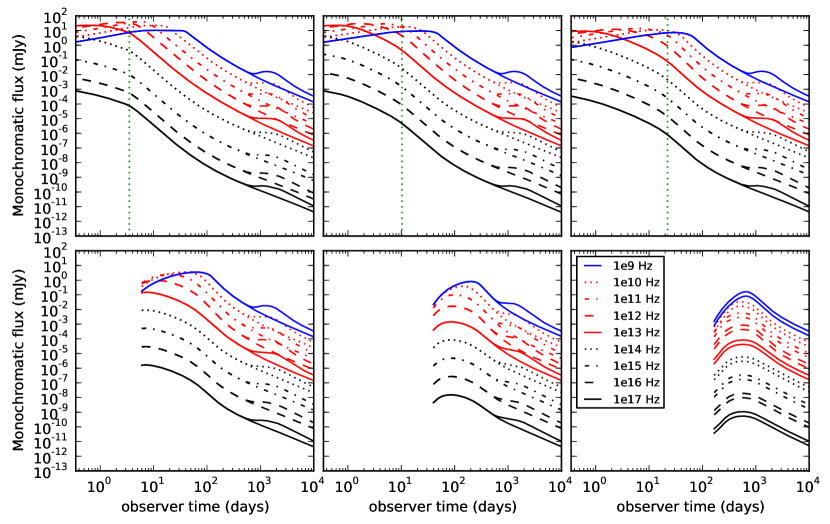
Figure 1.— Simulated light curves for various observer angles and frequencies. On the top row we have small observer angles, 0.0, 0.1 and 0.2 radians from left to right. On the bottom row we have large observer angles, 0.4, 0.8 and 1.57 radians from left to right. Observer frequencies from $10^{9}$ up to $10^{17}$ are plotted. For each frequency and angle a curve is plotted both with and without the contribution from the counterjet. The green vertical lines in the top plots indicate jet break time estimates using equation 4. The legend in the bottom right plot refers to all plots. Large observer angles are truncated at earlier time to show only observation times completely covered by the simulation.

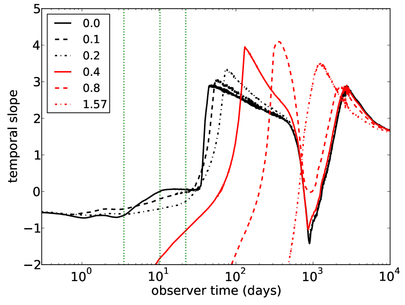
Figure 2.— Temporal decay index $\alpha$ assuming $F\propto t^{-\alpha}$. The observer frequency is $10^{9}$ Hz. The vertical lines at 3.5 days indicate the jet break time estimates for observers at 0, 0.1 and 0.2 radians (from left to right), using equation 4.

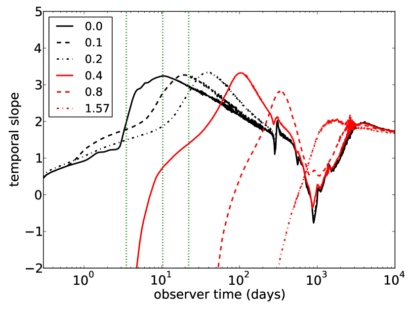
Figure 3.— Temporal decay index $\alpha$ assuming $F\propto t^{-\alpha}$. The observer frequency is $10^{17}$ Hz. The vertical lines at 3.5 days indicate the jet break time estimates for observers at 0, 0.1 and 0.2 radians (from left to right), using equation 4.

We first present the main results for both small and large observer angles, looking both at the light curves and the corresponding temporal slopes. An overview of light curves is shown in Fig. 1, where we have plotted multi-frequency light curves spanning from $10^{9}$ to $10^{17}$ Hz. The temporal slopes for the lowest frequency $10^{9}$ Hz and the highest frequency $10^{17}$ Hz are separately plotted in Figs. 2 and 3. For the on-axis results we estimate the jet break, a combination of lateral spreading and jet edges becoming visible, to occur around 3.5 days (the 7 days mentioned in ZM09 is for $z=1$). Direct comparisons at the same frequency of different observer angles are shown in figures 6 and 11, for 8.46 GHz. As the observer angle increases, the jet break splits into two for observers still inside the jet. Once the observer is positioned at the jet edge only one break remains that is significantly postponed. This effect is similar across all frequencies. The steepest drop in slope is the one associated with the edge of the jet furthest from the observer and can therefore be estimated to occur around

$$t_{j}=3.5(1+z)E_{iso,53}^{1/3}n_{1}^{-1/3}\left(\frac{\theta_{0}+\theta_{obs}}{0.2}\right)^{8/3}\textrm{ days},$$ (4)

where $E_{iso,53}$ is the isotropic equivalent energy in units of $10^{53}\,{\mathrm{erg}}$, $n_{1}$ is density of the medium in units of ${\mathrm{cm}}^{-3}$, $\theta_{0}$ is the jet half opening angle, and $\theta_{obs}$ is the observer angle relative to the jet axis. Jet breaks can be used to estimate the opening angles of GRB jets. It is usually assumed in GRB afterglow modeling that the observer is on the jet axis. However, if the observer is near the edge of the jet, the jet opening can be overestimated by a factor of up to 2, and the beaming-corrected total energy can be overestimated by a factor of up to 4. For a typical observer at $\theta_{obs}\approx 2\theta_{0}/3$, the beaming-corrected energy can be overestimated by a factor of $\sim 3$. The observational implications of this effect will be further discussed in Section 6.

At high observer angles, the rise of the light curve is postponed until the point where relativistic beaming has weakened sufficiently for the observer to be in the light cone of the radiating fluid. Due to limb-brightening the drop in temporal slope following a jet break initially overshoots its asymptotic value. After that it starts to change again due to the onset of the transition into the nonrelativistic regime and the rise of flux from the counterjet, before it finally settles into its asymptotic value for the nonrelativistic regime. In order to put the simulation results in context and to differentiate between the break due to lateral spreading and the break due to the edges becoming visible we will compare the simulation results against the BM solution for a hard edged jet without lateral spreading in the next subsection.

3.1. Afterglow emission for on-axis observer – hydrodynamic simulation versus analytic model

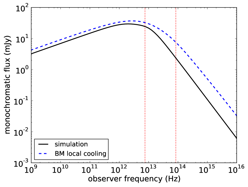
Figure 4.— direct comparison between on-axis spectrum from simulation (solid curve) and BM solution with locally calculated cooling times (dashed curve), omitting self-absorption. The spectra are taken at 1 day in observer time, so well before the jet break. The leftmost vertical dotted line denotes the analytically calculated position of $\nu_{m}$, the rightmost that of $\nu_{c}$ (calculated for the BM solution).

In Fig. 4 we show a comparison between on-axis spectra at 1 day in observer time, calculated from the simulation and from an analytical description using the BM solution plus synchrotron emission (Van Eerten & Wijers, 2009). The observed time is well before the jet break and before significant lateral spreading or slowing down of the jet has occurred. With the dynamics for both the simulation and the BM solution still being nearly equal, the figure therefore mainly shows the difference between the two approaches to synchrotron radiation. The differences below the cooling break $\nu_{c}$ are marginal and can be attributed to the absolute scaling of the emitted power. The difference beyond $\nu_{c}$ is significantly larger. The reason for this is that the simulation follows the approach to electron cooling from Sari et al. (1998), where the cooling time is globally estimated by setting it equal to the duration of the explosion, whereas Van Eerten & Wijers (2009) build upon Granot & Sari (2002) and calculate the local cooling time for each fluid element, which is given by the time passed since the fluid element has crossed the front of the shock. When the cooling time is calculated locally, the transition between pre- and post-cooling is smooth, with areas of the fluid further downstream making the transition before those at the front. Having the cooling time set globally results in a sudden global transition between the pre- and post-cooling regimes instead, with the same asymptotic spectral slope but a different value for the cooling break frequency and therefore a different absolute scaling of the flux for $\nu>\nu_{c}$. Note that even for a global cooling time, the sudden transition in the emission frame will still get smeared out in the observer frame.

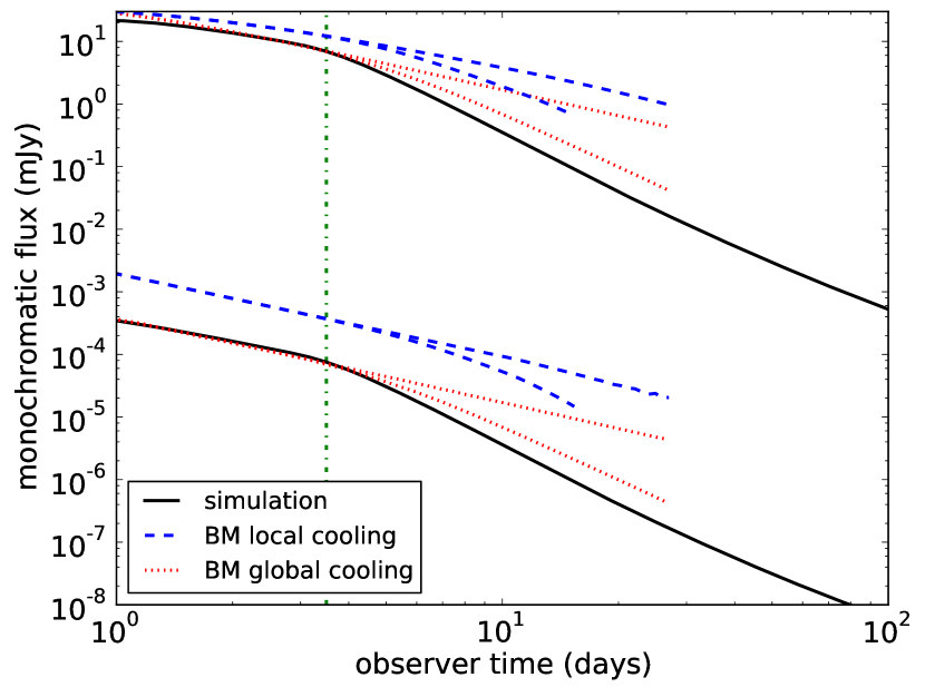
Figure 5.— Direct comparison of simulation results and heuristic description based on the Blandford-McKee exact solution. Simulated light curves are shown for observer frequencies $10^{13}$ and $10^{17}$ Hz (top and bottom solid line respectively). Analytical light curves are drawn for global (dashed) and local (dotted) cooling respectively. The top line of each pair is for a spherical model whereas the lower line is for a conic section only. The 3.5 days estimate for the jet break is indicated with a vertical dotted line.

Figure 5 shows a direct comparison between the on-axis light curves obtained from the simulation and light curves from the same analytical model as before. If no lateral spreading is assumed, a conic section of the spherically symmetric BM solution can be used to show the difference between the jet break due to the edges becoming visible and the combination of this break and the jet break due to lateral spreading. The exact light curves shown in Fig. 5 do not cover the entire observer time span because the BM solution ceases to be valid around a shock Lorentz factor of $\gamma\backsim 2$ (and slightly earlier for a local cooling calculation). The light curves are truncated at the point where this would start to affect the observed emission.

From the figure it can be seen that including lateral spreading has the effect that the jet break becomes steeper and starts slightly earlier (which confirms the low resolution comparison shown in Van Eerten et al. 2010b). The figure also shows the strong overshoot in steepening of the light curve following the jet break, also seen in Fig. 3. This overshoot has also been discussed in Granot et al. (2001) and ZM09.

The difference between the detailed local treatment of electron cooling and the global treatment of cooling is important when applying simulation results to actual data: it should be kept in mind that the simulation light curves systematically underestimate the flux beyond the cooling break. Electron cooling aside, the long term qualitative behavior of the light curve is fully captured by the simulation, with the results covering not only the relativistic regime but also the non-relativistic regime and the transition in between.

3.2. Afterglow emission for off-axis observer – hydrodynamic simulation versus analytic model

No exact solution exists that fully includes lateral spreading of the jet. In the Appendix we describe a simplified analytical model that approximates the behavior of the jet and allows us to calculate the observed flux for an observer at an arbitrary angle. Many such models exist in the literature (see e.g. Oren et al. (2004); Waxman (2004); Soderberg et al. (2006); Huang et al. (2007) etc.) and our model is not strongly different. Its distinguishing features are that it smoothly connects the relativistic BM solution to the nonrelativistic ST solution and that a conservative approach to lateral spreading is used where the jets start to spread at the speed of sound (and therefore logarithmically) upon approaching the nonrelativistic regime.

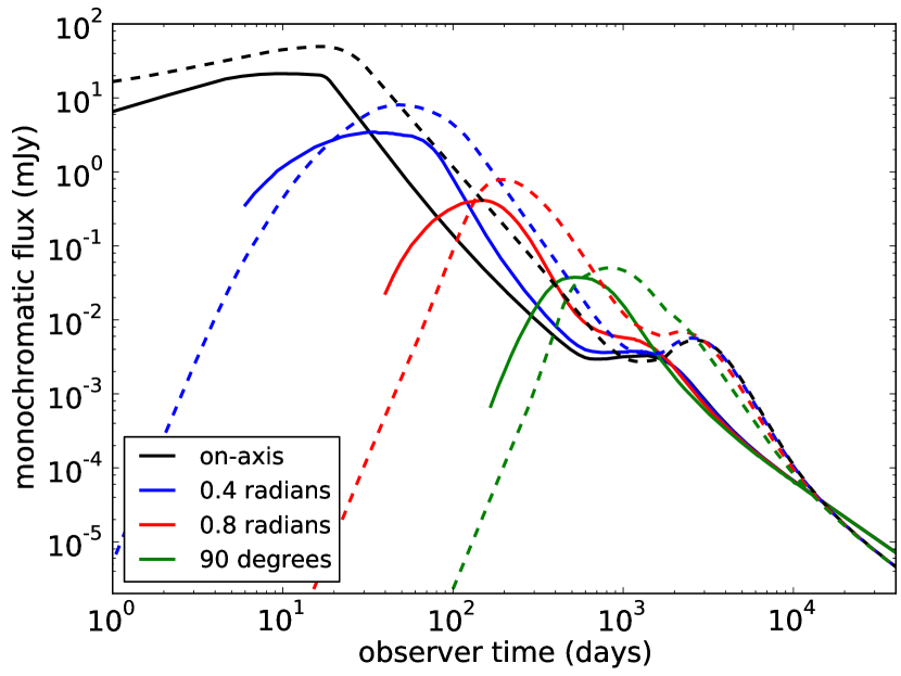
Figure 6.— Direct comparison between simulation results (solid lines) and analytical model (dashed lines) for different opening angles, for radio frequency 8.46 Ghz.

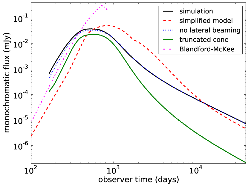
Figure 7.— Light curves at 8.46 Ghz for an observer at $\theta_{obs}=90^{\circ}$. The simulation and simplified model curves are repeated from fig. 6. If we ignore the fluid velocity in the lateral direction for the purpose of the radiation calculation, we get the slightly lower curve labeled no lateral beaming. The emission is still well in excess of a light curve from a radiation calculation that takes the BM profile instead of the simulated fluid profile as input, labeled Blandford-McKee. Only by completely omitting the emission contribution from matter that has spread sideways out of the original jet opening angle, we get a flux level that is initially comparable to that of the exact BM solution and the simplified model. This is shown by the truncated cone curve.

In figure 6 we show a comparison between off-axis light curves generated using the analytical model and light curves calculated from the simulation. Qualitatively both simulation and model show the same features. Quantitatively however, the differences are substantial. The simulation light curves peak earlier than the model light curves and do so at lower peak luminosity. At early times, the emission from off-axis simulation light curves is higher than that from the corresponding model light curves. The early time slopes for simulation and model light curves are similar. However, the further off-axis the observer, the later the observer time at which the simulation provides full coverage. In the figure, we have truncated the light curves at the observer time before which radiation from the blast wave with $\gamma>20$ would have been required. For two blast wave jets viewed sideways ($\theta_{obs}=90^{\circ}$), for example, full coverage starts beyond 100 days. This means that, even though the initial slopes agree between simulation and model, the early time shape of off-axis light curves in reality will be largely dictated by the initial shape of the blast wave, which does not need to be anything like the BM solution. Collapsar jet simulations indicate the existence of a cocoon around the emerging jet (see e.g., Zhang et al. 2003, 2004; Morsony et al. 2007; Mizuta & Aloy 2009).

We can understand why the off-axis light curves from the simulation are initially brighter than those from the simplified model by looking at one of the angles in more details. In Fig. 7 we have again plotted the simulation and model light curves for an observer at $\theta_{obs}=90^{\circ}$ (1.57 rad), together with a number of variations. We have now also included a light curve where we continue using the BM solution to determine the local fluid conditions, instead of the dynamical simulation results, but otherwise proceed as if we were reading the fluid quantities from disc (because of this, the curve also serves as a consistency check on the radiation calculation itself). The same approach has been used to generate the BM global cooling light curve in Fig. 5. The curve initially lies significantly below the simulation light curve. It also lies above the simplified model curve. The flux level of this BM curve is determined in part by the numerical resolution that we assume. In the plot we have used a resolution similar to that for the simulation curve, which initially resolves the radial profile with approximately 17 cells. Increasing the resolution moves the BM curve closer to the simplified slab curve, and not to the simulation curve. The difference between the BM curve and the simulation curve is real and we have added to the plot two hybrid simulation / model curves to make clear the cause of this difference.

First, when we completely ignore the velocity $v_{\theta}$ in the angular direction for the purpose of calculating the emission but otherwise still use the simulation dynamics, we find that the resulting light curve, labeled no lateral beaming in the figure, initially lies somewhat below the simulation curve before the two eventually merge. This tells us that part of the observed flux level is caused by beaming towards the observer of material spreading sideways, but that this is not the main cause of the difference between simulation and the hard edge jet models. At late times beaming no longer plays any role and the two curves are indeed no longer expected to be different.

The main reason for the difference is shown by the second additional curve. When calculating the light curve labeled truncated cone in the figure we have omitted the contribution to the radiation of any material that has spread sideways outside the original jet opening angle. The resulting curve lies very close to the BM light curve at first, before becoming orders of magnitude lower than all other curves. The late time behavior is as expected, for then only a small fraction of the energy and particle density is still contained within the original opening angle; the actual simulation flow has become roughly spherical. The early time behavior and the similarity between the truncated cone and BM light curves is more relevant. It demonstrates that the light curve for an off-axis observer is dominated by the emission from material that has spread sideways out of the original jet opening angle even though the energy of the material is very little and the sideways spreading is not yet dynamically important. In hindsight, the fact that the material on the side of the jet dominates the observed radio flux can easily be understood. It is not so much due to the fact that it moves a little faster towards the observer, for the $v_{\theta}$ component to the beaming is not that strong (as we have shown above). It is instead due to the fact that the radial velocity component $v_{r}$ drops quickly outside of the original jet opening angle and as a result the material outside the original jet opening angle is not beamed away from the observer as much as the material in the original jet cone. By contrast, for an on-axis observer the opposite is true and for a long time the received flux is dominated by emission from material inside the original jet opening angle. This has been demonstrated explicitly by Van Eerten et al. (2010b).

In the above sections we did not discuss the effects of synchrotron self-absorption. We will postpone addressing synchrotron self-absorption, which is not included in the simulation, until section 5.

4. Application: Hidden Jet Breaks?

A large number of X-ray afterglow light curves have been obtained by the Swift satellite since it was launched in 2004 (Gehrels et al., 2004). In a surprisingly large number of cases, these light curves fail to show a clearly discernable jet break (Racusin et al., 2009; Evans et al., 2009). Using our simulation results as a basis to generate synthetic Swift data sets for observers positioned at different angles from the jet axis, we show that the effect of observer position on the temporal evolution inferred from the data can be profound and sometimes render the jet break difficult to detect.

4.1. Procedure for creating synthetic data

The synthetic data sets that we produce should be comparable to those produced by the on-line Swift repository (Evans et al., 2007). Also they should have data points at a sufficiently late time that, if this were actual data, the jet break would be considered missing and not merely delayed. We therefore make sure that we have data up to at least 10 days, in accordance with the criteria for their ‘complete’ sample set by Racusin et al. (2009). The observed on-axis jet break for our simulation occurs roughly around three days. Synthetic light curves have also been created from an underlying model by Curran et al. (2008) (who find that even broken power law models observed on-axis can occasionally be mistaken for a single power law decline) and we follow the same procedure as described in that paper, changing only the time span and adding an additional late time data point if necessary. We then have:

• Constant counts and 1 $\sigma$ fractional error of 0.25 per data point.

• 94 minute orbits (47 min on/off due to Swift’s low-Earth orbit).

• Fractional exposure drops from 1.0 to 0.1 after one day (when Swift is usually no longer dedicated completely to observing the burst).

• Rate cut off at $5\times 10^{-4}$ cts/s.

• Observed number of cts/s is scaled to 0.1 at 1.0 day.

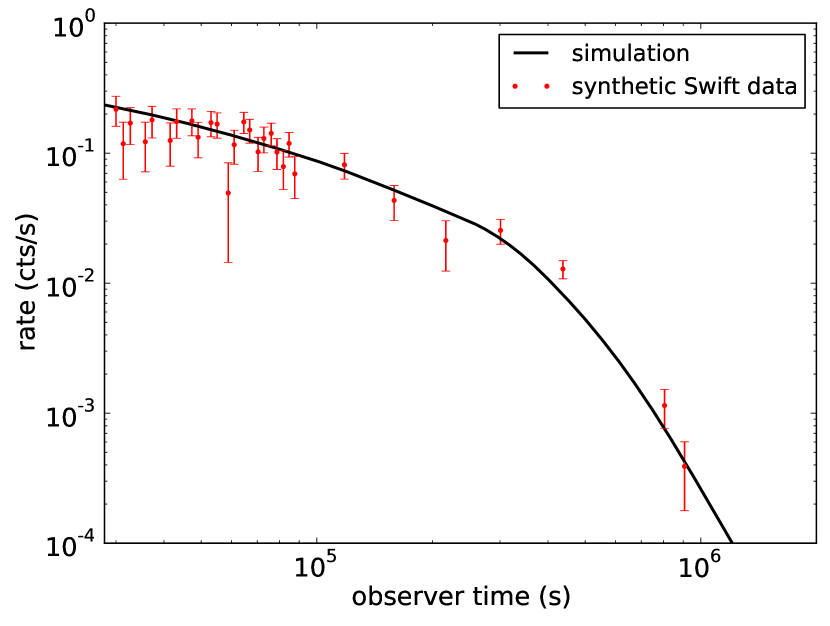
Figure 8.— Synthetic Swift data generated from simulation light curve for an on-axis observer and $p=2.5$. The simulation flux has been scaled to a count rate of 0.1 cts/s at 1 day observer time.

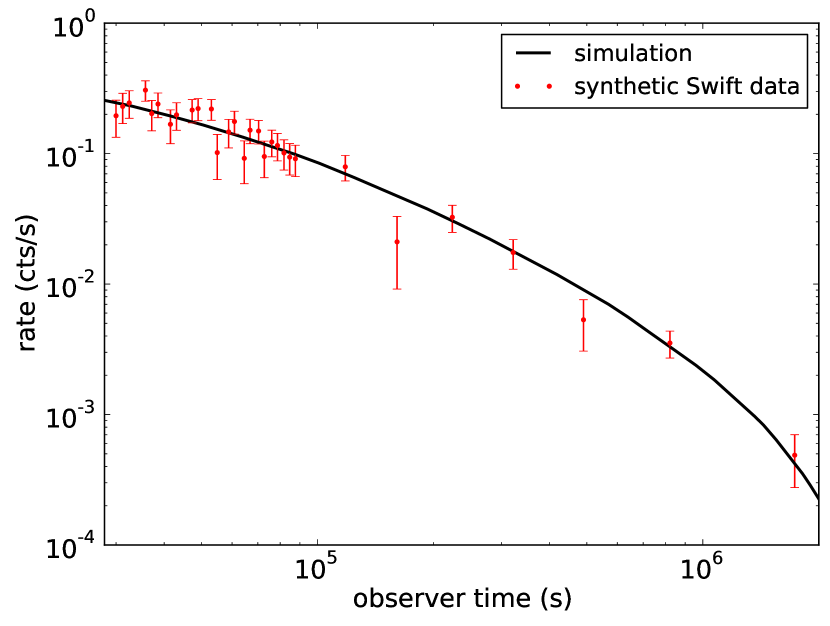
Figure 9.— Synthetic Swift data generated from simulation light curve for an on-edge observer (i.e. at 0.2 rad) and $p=2.5$. The simulation flux has been scaled to a count rate of 0.1 cts/s at 1 day observer time.

We start generating data points from $3\times 10^{4}$ s and continue until the rate drops below $5\times 10^{-4}$ cts/s. This starting point is chosen such that we have full coverage from the simulation at all observer angles under consideration. Like Curran et al. (2008), we increase the number of counts per bin to a number well in excess of the numbers mentioned by Evans et al. (2007). This has no physical significance but is used to generate synthetic light curves containing around 30 data points (The synthetic curves from Curran et al. contain more data points because they use an earlier starting time). If needed a late time data point is added to ensure that at least one data point is observed after ten days. The last one or two data points, where the count rates are less than $10^{-3}$ cts/s get a larger fractional error of 0.5. Out of the thousands of synthetic curves that have been generated, two randomly selected example synthetic light curves are shown in figures 8 and 9.

We generate light curves for observer angles 0.00, 0.02, 0.04, 0.06, 0.08, 0.1, 0.12, 0.14, 0.16, 0.18 and 0.2 radians. Note that by fixing the count rate at 0.1 cts/s after one day, we end up comparing on-axis observations to off-axis observations that are relatively brighter (i.e. corresponding to closer GRBs). As can be seen in Fig. 1, off-axis light curves are less bright than on-axis curves for the same physical parameters.

4.2. Fitting procedure and results

We follow Curran et al. (2008) again when fitting the synthetic data automatically using the simulated annealing method to minimise the $\chi^{2}$ of the residuals. The data are first fit to a single power law, then to a sharply broken power law,

$$F(t)=N\left\{\begin{array}[]{rl}(t/t_{b})^{-\alpha_{1}}&\text{if }t<t_{b},\\ (t/t_{b})^{-\alpha_{2}}&\text{if }t>t_{b}.\end{array}\right.$$ (5)

Curran et al. use a smooth power law, but a sharply broken power law is also used by Racusin et al. (2009). After each fit the count rates of the data points are re-perturbed from their original on-model values and a Monte Carlo analysis using 1000 trials is used to obtain average values and $1\sigma$ Gaussian deviations of the best fit parameters and F-test probabilities. This process is repeated for the list of observer angles mentioned previously. We have set $p=2.5$.

The F-test is a measure of the probability $F_{prob}$ that the decrease in $\chi^{2}$ associated with the addition of the two extra parameters of the broken power law, $\alpha_{2}$ and $t_{b}$, is by chance or not. When $F_{prob}\gtrsim 10^{-2}$ a single power law is commonly favored, when $10^{-5}\lesssim F_{prob}\lesssim 10^{-2}$ neither is favored but a single power law is usually presumed as the simpler model and when $F_{prob}\lesssim 10^{-5}$ a broken power law is favored.

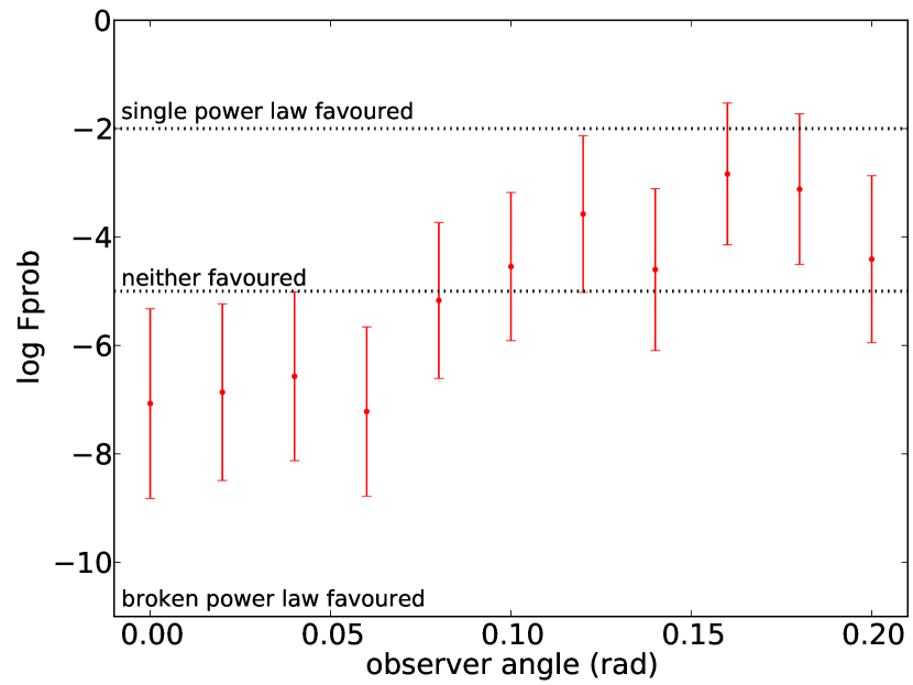
Figure 10.— Results for F-test as function of observer angle. Note that a typical observer angle is 0.13.

$\theta_{obs}$	$\alpha$	$\alpha_{1}$	$\alpha_{2}$	$t_{b}$ ($10^{5}$ s)
0.00	$1.69\pm 0.040$	$0.81\pm 0.16$	$3.32\pm 0.79$	$2.3\pm 0.80$
0.02	$1.68\pm 0.037$	$0.76\pm 0.17$	$3.14\pm 0.73$	$2.1\pm 0.83$
0.04	$1.63\pm 0.038$	$0.81\pm 0.15$	$2.96\pm 0.61$	$2.1\pm 0.72$
0.06	$1.78\pm 0.036$	$0.84\pm 0.16$	$3.05\pm 0.58$	$2.1\pm 0.70$
0.08	$1.52\pm 0.040$	$0.78\pm 0.19$	$2.26\pm 0.37$	$1.4\pm 0.54$
0.10	$1.51\pm 0.040$	$0.80\pm 0.20$	$2.07\pm 0.26$	$1.2\pm 0.45$
0.12	$1.49\pm 0.042$	$0.91\pm 0.26$	$1.95\pm 0.29$	$1.2\pm 0.55$
0.14	$1.65\pm 0.035$	$1.07\pm 0.16$	$2.36\pm 0.52$	$2.0\pm 1.1$
0.16	$1.46\pm 0.042$	$1.00\pm 0.28$	$1.95\pm 0.47$	$1.6\pm 0.89$
0.18	$1.40\pm 0.040$	$0.91\pm 0.36$	$1.85\pm 0.50$	$1.6\pm 0.97$
0.20	$1.42\pm 0.036$	$0.86\pm 0.21$	$2.01\pm 0.45$	$1.9\pm 1.0$

Table 1Average temporal power law slopes and jet break times $t_{b}$ for 1000 Monte Carlo iterations per observer angle $\theta_{obs}$. Here $\alpha$ denotes the single power law slope, $\alpha_{1}$ the pre-break broken power law slope and $\alpha_{2}$ the post-break broken power law slope.

$\theta_{obs}$	$\log(F_{prob})$	single	ambiguous	broken
0.00	$-7.1\pm 1.7$	0	130	870
0.02	$-6.9\pm 1.6$	0	148	852
0.04	$-6.6\pm 1.6$	0	202	798
0.06	$-7.2\pm 1.6$	0	60	940
0.08	$-5.2\pm 1.4$	6	510	484
0.10	$-4.5\pm 1.4$	22	698	280
0.12	$-3.6\pm 1.4$	129	767	104
0.14	$-4.6\pm 1.5$	21	641	338
0.16	$-2.8\pm 1.3$	274	675	51
0.18	$-3.1\pm 1.4$	259	686	55
0.20	$-4.4\pm 1.5$	37	663	300

Table 2Average $\log(F_{prob})$ values and classifications based on the criteria described in the text. For each angle, the classifications add up to 1000 Monte Carlo runs.

The results of the fitting procedure are shown in tables 1, 2 and fig. 10. In table 1 any slope $\alpha$ and its error $\Delta\alpha$ means that if an observer fits data to a swift dataset with similar count rate and duration and if the swift data was produced by an explosion that is accurately described by our numerical model, then that observer would find a slope that lies within $\Delta\alpha$ of $\alpha$ (the errors therefore do not reflect on the accuracy of the Monte Carlo run, which has converged to far greater precision). The analytically expected slopes for an on-axis observer and $p=2.5$ are 1.375 before and 2.125 after the jet break. These values are not even reproduced within $1\sigma$, which for the post-break slope can largely be attributed to the overshoot in slope directly after the break (see also section 3). Although the inaccuracy of the pre-break slope inferred from (synthetic) light curves will be smaller when earlier time data is available, which is often the case for Swift light curves, a systematic difference will remain (see also Jóhannesson et al. 2006). This emphasizes the importance of numerical modeling for the proper interpretation of Swift data. The situation gets worse when we move the observer off-axis. As Fig. 10 shows, even though a jet break is clearly detected on-axis for our physics settings, it can become hard to distinguish from a single power law for an observer positioned at $\theta_{j}/2$. The average observer angle one would expect when observing jets oriented randomly in the sky is $2\theta_{j}/3$ (for small jet opening angles, and assuming that the observer angle lies between zero and the jet opening angle). Larger observer angles will lead to orphan afterglows that we discuss separately below. It therefore follows that a significant number of jet breaks may remain hidden in the data due to the jets not being observed directly on-axis. In table 2 the classifications for the individual Monte Carlo iterations are also counted. Assuming again that jets are oriented randomly in the sky and that jets are only observed up to observer angles equal to $\theta_{j}$, we can calculate how often an afterglow with the physical parameters of the simulation would be classified as showing a jet break. For each angle $\theta_{i}$ we have classified $n_{i}$ out of 1000 synthetic curves as showing a jet break. This means that we will classify the afterglow described by the simulation as showing a jet break only $\sum_{i}n_{i}\sin(\theta_{i})/\sum_{i}1000\sin(\theta_{i})\times 100\%\approx 29\%$ of the time. This value is only a very rough estimate, for it depends on the $F_{prob}\lesssim 10^{-5}$ criterion, that is to some extent arbitrary. Also, as noted before, the off-axis curves are relatively brighter due to the fixed count rate. The requirement of having data up to ten days introduces a selection effect as well.

For all results above, it should be kept in mind that they have been obtained for a single half opening angle of 0.2 radians (approx. $11.5^{\circ}$) which is relatively large (although not extremely so and within the range of jet opening angles observationally inferred from Swift data). This results in a later jet break than a smaller opening angle would lead to. On the other hand we have set $z=0$, which again moves the jet break to earlier observer times and thereby compensates for the large opening angle. The general effect of higher observer angles is that both jet edges become observable at different times. The reason that a broken power law did not always produce a significantly better fit than a single power law is mainly because the full drop in count rate associated with the further edge got pushed out beyond ten days for off-axis observers (Section 3). For strongly collimated jets with small opening angles this effect is therefore expected to be less severe.

The often large difference between the physical parameters like $p$ (affecting the slope of the light curve) and $\theta_{j}$ (affecting the break time) used in a model and the values for these parameters when inferred from synthetic data created from that model has been discussed in detail by Jóhannesson et al. (2006). They also include the observer angle as a model parameter, but do not discuss it further in their paper.

5. Application: Orphan Afterglow Searches

The existence of orphan afterglows is an important and general prediction of current afterglow theories. Regardless of the GRB launching mechanism and the initial baryon content of the jet, eventually synchrotron emission from a decelerating baryonic blast wave should be observable for any observer angle. For this reason, various groups have looked for orphan afterglows, both at the optical and radio frequencies (e.g. Levinson et al. 2002; Gal-Yam et al. 2006; Soderberg et al. 2006; Malacrino et al. 2007). Few positive detections have been reported and surveys and archival studies have mainly served to establish constraints on GRB rates and beaming factors. Soderberg et al. (2006), for example, conclude from late time radio observations of 68 local type Ibc supernovae (SNe) that less than $\backsim 10\%$ of such SNe are associated with GRBs, and constrain the GRB beaming factor to be $\left<(1-\cos{\theta_{j}})^{-1}\right>\lesssim 10^{4}$. A lower limit to the beaming factor of $\left<(1-\cos{\theta_{j}})^{-1}\right>\gtrsim 13$ is provided by Levinson et al. (2002).

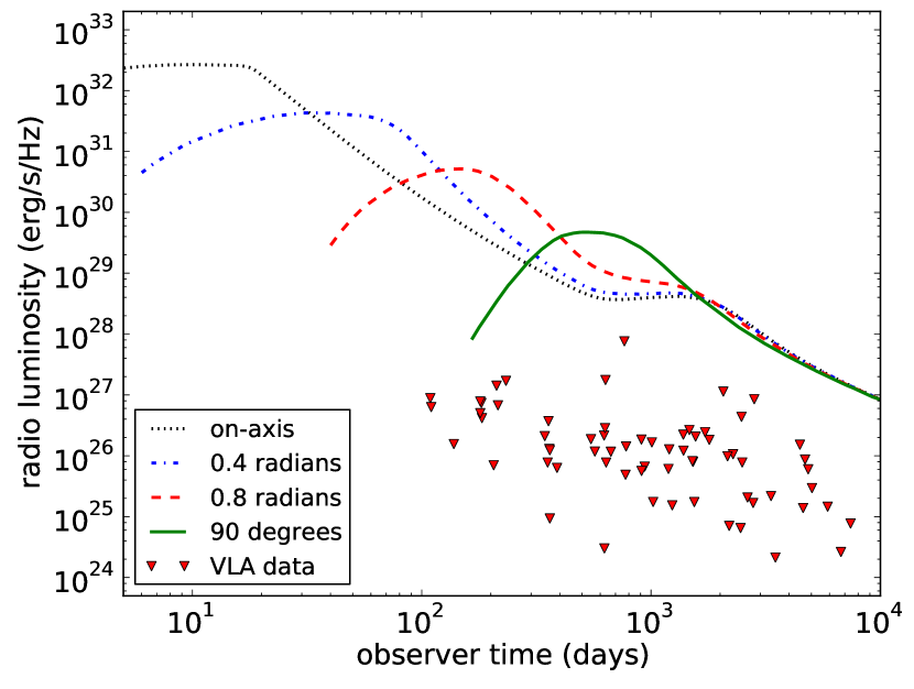
Figure 11.— VLA late time radio limits ($3\sigma$) for 66 local type Ibc of supernovae compared against simulation results. All supernova redshifts have been ignored (the largest redshift, that of SN 1991D, is $\backsim 0.04$). The fluxes have been rescaled to luminosities. All VLA observations were done at 8.46 GHz, the afterglow light curve is calculated at the same frequency. As in the rest of this paper, the simulation jet half opening angle is $11.5^{\circ}$.

Such estimates require a model describing the shape of off-axis light-curves, and are therefore sensitive to model assumptions. Eventually, comparing observations and detailed simulations like the one described in this paper will place the most accurate observational limits on orphan afterglow characteristics. A large number of simulations is required to fully explore the afterglow parameter space. We can however, use the single simulation of this paper that has typical values for the explosion parameters to confirm the result from Soderberg et al. (2006) that their sample of 68 supernovae observations are all significantly fainter than a standard afterglow viewed off-axis. This confirmation is shown in fig. 11, where we have plotted 66 supernovae radio upper limits (omitting SN 1984L and SN1954A, which were not observed at 8.46 GHz, from the original 68) together with our off-axis simulated light curves. Note that the jet half opening angle in our simulation is $11.5^{\circ}$, whereas Soderberg et al. (2006) use $5^{\circ}$. The fact that the early time flux received by an off-axis observer is actually stronger than analytically expected (as shown in section 3.2, where model and simulation are compared directly) only strengthens the case made by Soderberg et al.

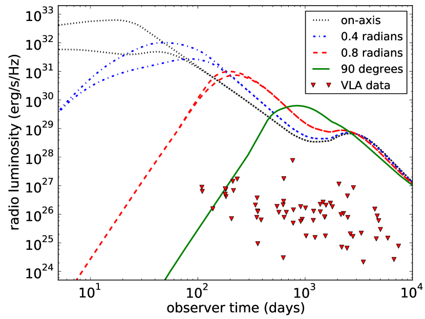
Figure 12.— Analytically calculated light curves for different observer angles, with and without self-absorption. The observer frequency is set at 8.46 GHz. Self-absorption influences the light curves only until a few hundred days at most. At 8.46 GHz, the light curve for an observer at 90 degrees is the same with and without self-absorption enabled. The jet half opening angle is $11.5^{\circ}$. The VLA late time radio limits for the local Ibc SNe are included as well.

A possible caveat to the above is that our simulation light curves do not include the effect of synchrotron self-absorption. Although we cannot completely rule out that this plays a role without actually calculating it, we can nevertheless look at the effect of self-absorption on the model light curves, having already established that model and simulation lead to at least qualitatively similar light curves in section 3.2. In Fig. 12 we show model light curves with and without synchrotron self-absorption, calculated as explained in the appendix. The figure shows that the effect of self-absorption is initially significant for an on-axis observer but becomes less pronounced for observers further off-axis. For an observer at $90^{\circ}$, the light curves with and without self-absorption are effectively identical. Aside from the minimal differences due to the analytical model assumptions, the main difference between this figure and fig. 1 from Soderberg et al. is due to the different jet opening angles. For our wider jet opening angle, only the two earliest supernovae lie clearly above the $90^{\circ}$ curve.

6. Summary and Discussion

In this paper we present broadband GRB afterglow light curves calculated assuming synchrotron emission from a high-resolution relativistic jet simulation in 2D. We have expanded the work presented in Zhang & MacFadyen (2009) to include observers positioned off the jet symmetry axis, both at small and large angles. For the jet simulation we have used the ram adaptive-mesh-refinement code, starting from the Blandford-McKee analytical solution and letting the jet evolve until it has reached the Sedov-Taylor stage and has decollimated into a nearly spherical outflow. We have implemented synchrotron radiation as described in Sari et al. (1998).

When put in the context of analytical light curve estimates, our simulations show the following:

• For an on-axis observer, the jet break from a 2D simulation including lateral spreading of the jet is seen earlier than that of a hard-edged jet. However, the break due to the jet edges becoming visible still dominates the shape of the light curve.

• We compared a description of electron cooling that takes into account the local cooling time since the shocked electrons passed the shock front to a description that uses a global cooling time estimate (as we have done in the simulation). The latter approach underestimates the observed cooling break frequency and therefore the post-break flux as well.

• The simulation light curves show that simplified homogeneous slab analytical models are qualitatively correct as long as they include a clear contribution from the counterjet for observers at all angles.

• Contrary to what has thus far been assumed in simplified analytical models and even though lateral spreading of the jet is initially not dynamically important, the received flux for an off-axis observer is strongly dominated by emission from material that has spread laterally outside the original jet opening angle. This is due to the fact that material outside the original jet cone has slowed done considerably in the radial direction and is therefore not beamed away from the observer as much as material closer to the jet axis.

• Moving the observer off-axis splits the jet break in two. The steep drop in slope only occurs after the break associated with the farthest edge and this break can thus be postponed until several weeks after the burst, even for observers positioned still within the jet cone. The late break time can be estimated by using the sum of the observer angle and the jet half opening angle instead of just the jet half opening angle.

In addition to these direct numerical results, we have presented two applications of our numerical work, one with observers positioned at small and moderate observer angles and one with observers at large observer angles.

• X-ray Light curves for observers at small observer angles are relevant for satellites such as Swift. Recent authors (e.g. Racusin et al. 2009; Evans et al. 2009) have noted a lack of jet breaks visible in the data. In order to check whether the observer angle can cause the jet break to remain hidden in the data we have performed a Monte Carlo analysis where we created synthetic Swift data out of simulation light curves for different observer angles. Observational biases and a Gaussian observational error were included. Broken and single power laws were then fit to the synthetic data sets. We found that it is not difficult to bury a jet break in the data for an off-axis observer. For our explosion parameters, even an observer at an angle of $\theta_{j}/2$ will not find a significantly better fit for a broken power law than for a single power law, leading to a missing jet break. For a random observer angle within the cone of the jet, a synthetic light curve created from our simulation will only show a discernable jet break 29 % of the time. Although our simulation is somewhat atypical in its above average initial opening angle of the jet, these results nevertheless imply that the observer angle has a strong influence on the interpretation of X-ray data. This holds even for observers still within the cone of the jet, observer angles that have usually been ignored and considered practically on-axis.

• As a second application we have confirmed the result of Soderberg et al. (2006) that a sample of 68 nearby type Ibc SNe cannot harbor an off-axis GRB, at least for the typical afterglow parameters that we have used for our simulation. This confirms the observational restrictions placed on orphan afterglow rate and beaming factor by these and other authors. The fact that at early times the light curves for off-axis observers are actually brighter than analytically expected, even strengthens the conclusions of Soderberg et al. (2006).

Recent deep late-time optical observations by Dai et al. (2008) have detected jet breaks in several bursts and they suggest that the lack of jet breaks in Swift bursts is due to the lack of well sampled light curves at late times. Therefore they conclude that the collimated outflow model GRBs is still valid. However, the non-detection of a jet break or a break at very late times in several GRBs (050904, Cenko et al. 2010b; 070125, Cenko et al. 2010b; 080319B, Cenko et al. 2010b; 080721, Starling et al. 2009; 080916C, Greiner et al. 2009; 090902B, Pandey et al. 2010; 090926A, Cenko et al. 2010a) seems to infer a huge amount of released energy ($\gtrsim 10^{52}\,\mathrm{erg}$) in these bursts. This leads Cenko et al. (2010b, a) to propose a class of hyper-energetic GRBs and challenge the magnetar model for GRBs (Usov, 1992; Duncan & Thompson, 1992; Thompson et al., 2004; Uzdensky & MacFadyen, 2007; Komissarov & Barkov, 2007; Bucciantini et al., 2009). Although hyper-energetic GRBs might exist, we propose an alternate explanation, in which the observer is simply off-axis. Note that an observer is more likely to be off-axis than on-axis. A typical observer sees the burst from $\theta_{obs}\approx 2\theta_{0}/3$ so is closer to the jet edge than jet axis. Applying an on-axis model to a jet that is seen off-axis will overestimate the total energy release by a factor of up to 4 because the jet break can be delayed by a factor of up to $\sim 6$ (see Eq. 4). We emphasize that when the jet opening angle is corrected for off-axis observer angle, the inferred energy release of those hyper-energetic events can be revised downwards by factors of several lessening tension with magnetar models for the GRB central engine.

These are the main conclusions of the work presented in this paper. In addition to this, the current results also raise a number of issues that need to be addressed in future work. Our simulation results can be generalized by performing additional simulations. And given the quantitative differences between simulation and simplified analytical models (such as the homogeneous slab model described in the Appendix), this is expected to result in different constraints on orphan afterglow rate and beaming factor. We have so far ignored self-absorption when calculating light curves. A simplified homogeneous slab approximation indicates that self-absorption is not expected to play a large role for observers at high angles. The applicability of our analytical model is however limited, especially in view of our finding that the early flux received by an off-axis observer is dominated by emission from material that has spread sideways and has slowed down more than material on the jet axis. It is conceivable that emission from this material has different spectral properties. Finally, the significant difference in observed flux between two approaches to synchrotron cooling that we have discussed emphasize the importance of a detailed model for the microphysics and radiation mechanisms involved.

Appendix A Summary of analytical model

Here we provide a short summary of our analytical model. In this model, light curves are calculated by numerical integration over an infinitesimally thin homogeneous blast wave front. The received flux is given by

$$F=\frac{1}{4\pi d^{2}_{L}}\int d^{3}\mathbf{r}\frac{\epsilon^{\prime}_{\nu^{\prime}}}{\gamma^{2}(1-\beta\mu)^{2}},$$ (A1)

when we ignore the redshift $z$. Here $\epsilon^{\prime}_{\nu^{\prime}}$ is the comoving frame emissivity and $\mu$ the angle between observer direction and local velocity. The dependence of the beaming and emissivity on the observer time $t_{obs}$ is kept implicit (see also eqn. A8; the volume integral needs to be taken across different emission times). Assuming the radiation is produced by an infinitesimally thin shell with width $\Delta R$ we get

$$F=\frac{1}{4\pi d^{2}_{L}}\int d\theta d\phi R^{2}\sin{\theta}\Delta R\frac{\epsilon^{\prime}_{\nu^{\prime}}}{\gamma^{2}(1-\beta\mu)^{2}},$$ (A2)

For every observer time we integrate over jet angles $\theta$ and $\phi$ (we define $\theta$ such that it is not the angle between observer and local fluid velocity, but that between local fluid velocity and jet axis), while taking into account that radiation from different emission angles.

The emissivity can be calculated from the local fluid conditions, which we know in turn in terms of emission time $t_{e}$. For the blast wave radius we have by definition:

$$R=c\int\beta_{sh}dt_{e},$$ (A3)

Where the subscript $sh$ indicates shock velocity. From the shock jump conditions it follows for arbitrary strong shocks that

$$e^{\prime}_{th}=(\gamma-1)n^{\prime}m_{p}c^{2}.$$ (A4)

The comoving downstream number density $n^{\prime}$ in both the relativistic and nonrelativistic regime is given by

$$n^{\prime}=4n_{0}\gamma,$$ (A5)

with $\gamma\to 1$ in the nonrelativistic limit. We assume this equation to remain valid in the intermediate regime as well. This is not implied by the expression above, where we have kept implicit the dependence on the fluid adiabatic index (which changes from $4/3$ to $5/3$ over the course of the blast wave evolution).

We set the width of the shell at a single emission time by demanding that the shell contains all swept-up particles, leading to:

$$4\pi\left[R_{f}(t_{f})-R_{b}(t_{f})\right]R^{2}n=4/3\pi R^{3}n_{0}\to\left[R_{f}(t_{f})-R_{b}(t_{f})\right]=\frac{R}{12\gamma^{2}},$$ (A6)

where we have used $n=\gamma n^{\prime}=4n_{0}\gamma^{2}$, again assumed valid throughout the entire evolution of the fluid. The subscript $f$ denotes the front of the shock and the subscript $b$ denotes the back of the shock. Setting the shock width through the number of particles is to some extent an arbitrary choice, and we could also have used the total energy which would have yielded a different width (since the downstream energy density profile is different from the downstream number density profile). The width of the shell $\Delta R$ in equation A2 has to take into account the emission time difference between the front and back of the shell and is given by

$$\Delta R=|R_{f}(t_{f})-R_{b}(t_{b})|=|R_{f}(t_{f})-R_{f}(t_{b})\left[1-\frac{1}{12\gamma(t_{b})^{2}}\right]|.$$ (A7)

Because the shell is very thin, $R_{f}(t_{b})\approx R_{f}(t_{f})-\beta_{sh}c\Delta t$. We integrate over emission arriving at a single observer time, and for given values of $\mu$ and $t_{obs}$ we have

$$t_{obs}=t_{f}-\mu R_{f}(t_{f})/c=t_{b}-\mu R_{b}(t_{b})/c,$$ (A8)

which yields $\Delta R=\Delta tc/\mu$ when differentiated. Combining the above, we eventually find

$$\Delta R=\frac{1}{1-\beta_{sh}\mu}\cdot\frac{R}{12\gamma^{2}}.$$ (A9)

For the shock velocity we have

$$(\beta_{sh}\gamma_{sh})_{BM}=\left(\frac{17\cdot E_{\mathrm{iso}}}{8\pi n_{0}m_{p}c^{5}}\right)^{1/2}t_{e}^{-3/2}\equiv C_{BM}t_{e}^{-3/2};\qquad(\beta_{sh}\gamma_{sh})_{ST}=\frac{2}{5}\cdot 1.15\cdot\left(\frac{E_{j}}{n_{0}m_{p}c^{5}}\right)^{1/5}\cdot t_{e}^{-3/5}\equiv C_{ST}\cdot t_{e}^{-3/5},$$ (A10)

in the BM and ST regime respectively. We artificially combine the two simply by adding them (after squaring):

$$\beta_{sh}^{2}\gamma_{sh}^{2}=C^{2}_{BM}t_{e}^{-3}+C^{2}_{ST}t_{e}^{-6/5}.$$ (A11)

Note that the BM quantities depend on $E_{iso}$, while the ST quantities depend on $E_{j}$. The two are related via $E_{j}=E_{iso}\theta_{j}^{2}/2$. Here $E_{j}$ is the total energy in both jets, and $\theta_{j}$ the half opening angle of a jet. The fluid Lorentz factor in the relativistic regime is related to the shock Lorentz factor via $\gamma^{2}=\gamma_{sh}^{2}/2$, while the fluid velocity in the non-relativistic regime is related to the shock velocity via $\beta=3/4\beta_{sh}$. We therefore construct a relationship between emission time and fluid velocity similar to that between emission time and shock velocity:

$$\beta^{2}\gamma^{2}=\frac{1}{2}C_{BM}^{2}t_{e}^{-3}+\frac{9}{16}C_{ST}^{2}t_{e}^{-6/5}.$$ (A12)

We assume that the jet does not spread sideways throughout the relativistic phase of its evolution. However, at some point the blast wave must become spherical. For if we keep the opening angle fixed, but do take $E_{j}$ to dictate the ST solution instead of $E_{iso}$ we would underestimate the final flux by integrating over an integration domain that is too small. We will assume that the jet starts spreading sideways when it has reached the nonrelativistic phase and we take this moment to be given by

$$(\beta\gamma)_{BM}=1\to t_{NR}=2^{1/3}C_{BM}^{2/3}.$$ (A13)

At this point, the jet starts spreading sideways with the speed of sound $c_{s}$, leading to

$$R\frac{d\theta}{dt_{obs}}=c_{s}.$$ (A14)

In the nonrelativistic regime $dt_{obs}$ and $dt_{e}$ are identical. The ST solution for the speed of sound for adiabatic index $5/3$ is given by $c_{s}=r/\sqrt{20}t$, leading to

$$\theta=\theta_{j}+\frac{1}{\sqrt{20}}\ln\frac{t_{obs}}{t_{NR}},$$ (A15)

until spherical symmetry is reached. By contrast, Rhoads ’99 take $\Omega\approx\pi(\theta_{j}+c_{s}t^{\prime}/ct_{e})^{2}$ (where $t^{\prime}$ time in the comoving frame, and $\Omega$ a solid angle) as the starting point.

From the local fluid conditions the local emissivity can be calculated. In the case of slow cooling, we define

$$\epsilon^{\prime}_{\nu^{\prime}} = \epsilon^{\prime}_{m}\left(\frac{\nu^{\prime}}{\nu^{\prime}_{m}}\right)^{1/3},\qquad\nu^{\prime}<\nu^{\prime}_{m}$$

$$\epsilon^{\prime}_{\nu^{\prime}} = \epsilon^{\prime}_{m}\left(\frac{\nu^{\prime}}{\nu^{\prime}_{m}}\right)^{(1-p)/2},\qquad\nu^{\prime}_{m}<\nu^{\prime}<\nu^{\prime}_{c}$$

$$\epsilon^{\prime}_{\nu^{\prime}} = \epsilon^{\prime}_{m}\left(\frac{\nu^{\prime}_{c}}{\nu^{\prime}_{m}}\right)^{(1-p)/2}\left(\frac{\nu^{\prime}}{\nu^{\prime}_{c}}\right)^{-p/2},\qquad\nu^{\prime}_{c}<\nu^{\prime}.$$ (A16)

The definition for fast cooling is analogous (see also Sari et al. 1998). The peak emissivity is given by

$$\epsilon^{\prime}_{m}\backsim\frac{p-1}{2}\frac{\sqrt{3}q_{e}^{3}}{m_{e}c^{2}}n^{\prime}B^{\prime}.$$ (A17)

The synchrotron break frequency $\nu^{\prime}_{m}$ depends on its corresponding critical electron Lorentz factor $\gamma^{\prime}_{m}$, leading to

$$\nu^{\prime}_{m}=\frac{3}{4\pi}\frac{q_{e}}{m_{e}c}(\gamma^{\prime}_{m})^{2}B^{\prime},\qquad\gamma^{\prime}_{m}=\left(\frac{p-2}{p-1}\right)\frac{\epsilon_{e}e^{\prime}_{th}}{n^{\prime}m_{e}c^{2}}.$$ (A18)

For the cooling break frequency an identical relation between frequency and electron Lorentz factor holds. The critical Lorentz factor is now given by

$$\gamma^{\prime}_{c}=\frac{6\pi m_{e}\gamma c}{\sigma_{T}(B^{\prime})^{2}t_{e}},$$ (A19)

which follows from the electron kinetic equation when synchrotron losses dominate over adiabatic expansion and the cooling time is approximated by the lab frame time since the explosion.

Synchrotron self-absorption is included in the model using the assumption that emission and absorption occur in a homogeneous shell. The solution to the linear equation of radiative transfer then dictates that we need to replace eq. A2 by

$$F=\frac{1}{4\pi d^{2}_{L}}\int d\theta d\phi R^{2}\sin{\theta}\frac{\epsilon_{\nu}}{\alpha_{\nu}}(1-\mathrm{e}^{-\tau}),$$ (A20)

The optical depth $\tau\approx-\alpha_{\nu}\Delta R$ . Emissivity and absorption translate between frames using $\epsilon^{\prime}_{\nu^{\prime}}=\gamma^{2}(1-\beta\mu)^{2}\epsilon_{\nu}$ and $\alpha^{\prime}_{\nu^{\prime}}=\alpha_{\nu}/\gamma(1-\beta\mu)$ respectively. In our simplified model we calculate the absorption coefficient $\alpha^{\prime}_{\nu^{\prime}}$ under the assumption that electron cooling does not influence it. This assumption is justified when the self-absorption break frequency $\nu_{a}$ lies well below the cooling break frequency $\nu_{c}$, which is the case for all applications of the model in this paper. Also approximating the synchrotron spectral shape by just two sharply connected power laws we then find for the self-absorption coefficient:

$$\alpha^{\prime}_{\nu^{\prime}}=(p-1)(p+2)n^{\prime}\frac{\sqrt{3}q_{e}^{3}B^{\prime}}{\gamma^{\prime}_{m}16\pi m_{e}^{2}c^{2}}(\nu^{\prime})^{-2}\left(\frac{\nu^{\prime}}{\nu^{\prime}_{m}}\right)^{\kappa},$$ (A21)

where $\kappa=1/3$ if $\nu^{\prime}<\nu^{\prime}_{m}$ and $\kappa=-p/2$ otherwise.

Numerically speaking the integration procedure is as follows. First we tabulate $R(t_{e})$ for a given set of physical parameters, so that we do not need to estimate it analytically but can use its exact dependence on the fluid Lorentz factor instead. We integrate over $\theta$ before we integrate over $\phi$, and for each $\theta$, $\phi$ the angle between observer and fluid element is given by

$$\mu=\sin{\theta}\cos{\phi}\sin{\theta_{obs}}+\cos{\theta}\cos{\theta_{obs}}.$$ (A22)

Having tabulated $R(t_{e})$, we tabulate $\mu(t_{e},R(t_{e}))$ as well for a given value of $t_{obs}$. Since $\mu(t_{e})$ is a monotonically increasing function of $t_{e}$, we can unambiguously determine $t_{e}(\mu)$ from this table. When determining the value of the integrand at a given value of $\theta$, $\phi$, we can now calculate the local fluid conditions and emissivity via $t_{e}(\mu(\theta,\phi))$.

References

- Blandford & McKee (1976) Blandford, R. D. & McKee, C. F. 1976, Physics of Fluids, 19, 1130
- Bucciantini et al. (2009) Bucciantini, N., Quataert, E., Metzger, B. D., Thompson, T. A., Arons, J., & Del Zanna, L. 2009, MNRAS, 396, 2038
- Cenko et al. (2010a) Cenko, S. B., Frail, D. A., Harrison, F. A., Haislip, J. B., Reichart, D. E., Butler, N. R., Cobb, B. E., Cucchiara, A., Berger, E., Bloom, J. S., Chandra, P., Fox, D. B., Perley, D. A., Prochaska, J. X., Filippenko, A. V., Glazebrook, K., Ivarsen, K. M., Kasliwal, M. M., Kulkarni, S. R., LaCluyze, A. P., Lopez, S., Morgan, A. N., Pettini, M., & Rana, V. R. 2010a, ArXiv e-prints, arXiv:1004.2900
- Cenko et al. (2010b) Cenko, S. B., Frail, D. A., Harrison, F. A., Kulkarni, S. R., Nakar, E., Chandra, P. C., Butler, N. R., Fox, D. B., Gal-Yam, A., Kasliwal, M. M., Kelemen, J., Moon, D., Ofek, E. O., Price, P. A., Rau, A., Soderberg, A. M., Teplitz, H. I., Werner, M. W., Bock, D., Bloom, J. S., Starr, D. A., Filippenko, A. V., Chevalier, R. A., Gehrels, N., Nousek, J. N., & Piran, T. 2010b, ApJ, 711, 641
- Curran et al. (2008) Curran, P. A., van der Horst, A. J., & Wijers, R. A. M. J. 2008, MNRAS, 386, 859
- Dai et al. (2008) Dai, X., Garnavich, P. M., Prieto, J. L., Stanek, K. Z., Kochanek, C. S., Bechtold, J., Bouche, N., Buschkamp, P., Diolaiti, E., Fan, X., Giallongo, E., Gredel, R., Hill, J. M., Jiang, L., McClelland, C., Milne, P., Pedichini, F., Pogge, R. W., Ragazzoni, R., Rhoads, J., Smareglia, R., Thompson, D., & Wagner, R. M. 2008, ApJ, 682, L77
- Downes et al. (2002) Downes, T. P., Duffy, P., & Komissarov, S. S. 2002, MNRAS, 332, 144
- Duncan & Thompson (1992) Duncan, R. C. & Thompson, C. 1992, ApJ, 392, L9
- Evans et al. (2009) Evans, P. A., Beardmore, A. P., Page, K. L., Osborne, J. P., O’Brien, P. T., Willingale, R., Starling, R. L. C., Burrows, D. N., Godet, O., Vetere, L., Racusin, J., Goad, M. R., Wiersema, K., Angelini, L., Capalbi, M., Chincarini, G., Gehrels, N., Kennea, J. A., Margutti, R., Morris, D. C., Mountford, C. J., Pagani, C., Perri, M., Romano, P., & Tanvir, N. 2009, MNRAS, 397, 1177
- Evans et al. (2007) Evans, P. A., Beardmore, A. P., Page, K. L., Tyler, L. G., Osborne, J. P., Goad, M. R., O’Brien, P. T., Vetere, L., Racusin, J., Morris, D., Burrows, D. N., Capalbi, M., Perri, M., Gehrels, N., & Romano, P. 2007, A&A, 469, 379
- Fryxell et al. (2000) Fryxell, B., Olson, K., Ricker, P., Timmes, F. X., Zingale, M., Lamb, D. Q., MacNeice, P., Rosner, R., Truran, J. W., & Tufo, H. 2000, ApJS, 131, 273
- Gal-Yam et al. (2006) Gal-Yam, A., Ofek, E. O., Poznanski, D., Levinson, A., Waxman, E., Frail, D. A., Soderberg, A. M., Nakar, E., Li, W., & Filippenko, A. V. 2006, ApJ, 639, 331
- Gehrels et al. (2004) Gehrels, N., Chincarini, G., Giommi, P., Mason, K. O., Nousek, J. A., Wells, A. A., White, N. E., Barthelmy, S. D., Burrows, D. N., Cominsky, L. R., Hurley, K. C., Marshall, F. E., Mészáros, P., Roming, P. W. A., Angelini, L., Barbier, L. M., Belloni, T., Campana, S., Caraveo, P. A., Chester, M. M., Citterio, O., Cline, T. L., Cropper, M. S., Cummings, J. R., Dean, A. J., Feigelson, E. D., Fenimore, E. E., Frail, D. A., Fruchter, A. S., Garmire, G. P., Gendreau, K., Ghisellini, G., Greiner, J., Hill, J. E., Hunsberger, S. D., Krimm, H. A., Kulkarni, S. R., Kumar, P., Lebrun, F., Lloyd-Ronning, N. M., Markwardt, C. B., Mattson, B. J., Mushotzky, R. F., Norris, J. P., Osborne, J., Paczynski, B., Palmer, D. M., Park, H., Parsons, A. M., Paul, J., Rees, M. J., Reynolds, C. S., Rhoads, J. E., Sasseen, T. P., Schaefer, B. E., Short, A. T., Smale, A. P., Smith, I. A., Stella, L., Tagliaferri, G., Takahashi, T., Tashiro, M., Townsley, L. K., Tueller, J., Turner, M. J. L., Vietri, M., Voges, W., Ward, M. J., Willingale, R., Zerbi, F. M., & Zhang, W. W. 2004, ApJ, 611, 1005
- Granot (2007) Granot, J. 2007, in Revista Mexicana de Astronomia y Astrofisica Conference Series, Vol. 27, Revista Mexicana de Astronomia y Astrofisica, vol. 27, 140–165
- Granot et al. (2001) Granot, J., Miller, M., Piran, T., Suen, W. M., & Hughes, P. A. 2001, in Gamma-ray Bursts in the Afterglow Era, ed. E. Costa, F. Frontera, & J. Hjorth, 312–+
- Granot et al. (2002) Granot, J., Panaitescu, A., Kumar, P., & Woosley, S. E. 2002, ApJ, 570, L61
- Granot & Sari (2002) Granot, J. & Sari, R. 2002, ApJ, 568, 820
- Greiner et al. (2009) Greiner, J., Clemens, C., Krühler, T., von Kienlin, A., Rau, A., Sari, R., Fox, D. B., Kawai, N., Afonso, P., Ajello, M., Berger, E., Cenko, S. B., Cucchiara, A., Filgas, R., Klose, S., Küpcü Yoldaş, A., Lichti, G. G., Löw, S., McBreen, S., Nagayama, T., Rossi, A., Sato, S., Szokoly, G., Yoldaş, A., & Zhang, X. 2009, A&A, 498, 89
- Huang et al. (2007) Huang, Y., Lu, Y., Wong, A. Y. L., & Cheng, K. S. 2007, Chinese Journal of Astronomy and Astrophysics, 7, 397
- Jiang & Shu (1996) Jiang, G. & Shu, C. 1996, Journal of Computational Physics, 126, 202
- Jóhannesson et al. (2006) Jóhannesson, G., Björnsson, G., & Gudmundsson, E. H. 2006, ApJ, 640, L5
- Kobayashi et al. (1999) Kobayashi, S., Piran, T., & Sari, R. 1999, ApJ, 513, 669
- Komissarov & Barkov (2007) Komissarov, S. S. & Barkov, M. V. 2007, MNRAS, 382, 1029
- Kumar & Panaitescu (2000) Kumar, P. & Panaitescu, A. 2000, ApJ, 541, L51
- Levinson et al. (2002) Levinson, A., Ofek, E. O., Waxman, E., & Gal-Yam, A. 2002, ApJ, 576, 923
- MacNeice et al. (2000) MacNeice, P., Olson, K. M., Mobarry, C., de Fainchtein, R., & Packer, C. 2000, Computer Physics Communications, 126, 330
- Malacrino et al. (2007) Malacrino, F., Atteia, J.-L., Boër, M., Klotz, A., Veillet, C., Cuillandre, J.-C., & The Grb Rtas Collaboration. 2007, A&A, 464, L29
- Meliani et al. (2007) Meliani, Z., Keppens, R., Casse, F., & Giannios, D. 2007, MNRAS, 376, 1189
- Mészáros (2006) Mészáros, P. 2006, Reports on Progress in Physics, 69, 2259
- Mimica et al. (2009) Mimica, P., Giannios, D., & Aloy, M. A. 2009, A&A, 494, 879
- Mizuta & Aloy (2009) Mizuta, A. & Aloy, M. A. 2009, ApJ, 699, 1261
- Morsony et al. (2007) Morsony, B. J., Lazzati, D., & Begelman, M. C. 2007, ApJ, 665, 569
- Oren et al. (2004) Oren, Y., Nakar, E., & Piran, T. 2004, MNRAS, 353, L35
- Pandey et al. (2010) Pandey, S. B., Swenson, C. A., Perley, D. A., Guidorzi, C., Wiersema, K., Malesani, D., Akerlof, C., Ashley, M. C. B., Bersier, D., Cano, Z., Gomboc, A., Ilyin, I., Jakobsson, P., Kleiser, I. K. W., Kobayashi, S., Kouveliotou, C., Levan, A. J., McKay, T. A., Melandri, A., Mottram, C. J., Mundell, C. G., O’Brien, P. T., Phillips, A., Rex, J. M., Siegel, M. H., Smith, R. J., Steele, I. A., Stratta, G., Tanvir, N. R., Weights, D., Yost, S. A., Yuan, F., & Zheng, W. 2010, ApJ, 714, 799
- Piran (2005) Piran, T. 2005, Reviews of Modern Physics, 76, 1143
- Racusin et al. (2009) Racusin, J. L., Liang, E. W., Burrows, D. N., Falcone, A., Sakamoto, T., Zhang, B. B., Zhang, B., Evans, P., & Osborne, J. 2009, ApJ, 698, 43
- Rhoads (1997) Rhoads, J. E. 1997, ApJ, 487, L1
- Rhoads (1999) —. 1999, ApJ, 525, 737
- Rossi et al. (2008) Rossi, E. M., Perna, R., & Daigne, F. 2008, MNRAS, 390, 675
- Sari et al. (1998) Sari, R., Piran, T., & Narayan, R. 1998, ApJ, 497, L17+
- Sedov (1959) Sedov, L. I. 1959, Similarity and Dimensional Methods in Mechanics (Similarity and Dimensional Methods in Mechanics, New York: Academic Press, 1959)
- Soderberg et al. (2006) Soderberg, A. M., Nakar, E., Berger, E., & Kulkarni, S. R. 2006, ApJ, 638, 930
- Starling et al. (2009) Starling, R. L. C., Rol, E., van der Horst, A. J., Yoon, S., Pal’Shin, V., Ledoux, C., Page, K. L., Fynbo, J. P. U., Wiersema, K., Tanvir, N. R., Jakobsson, P., Guidorzi, C., Curran, P. A., Levan, A. J., O’Brien, P. T., Osborne, J. P., Svinkin, D., de Ugarte Postigo, A., Oosting, T., & Howarth, I. D. 2009, MNRAS, 400, 90
- Taylor (1950) Taylor, G. 1950, Royal Society of London Proceedings Series A, 201, 159
- Thompson et al. (2004) Thompson, T. A., Chang, P., & Quataert, E. 2004, ApJ, 611, 380
- Usov (1992) Usov, V. V. 1992, Nature, 357, 472
- Uzdensky & MacFadyen (2007) Uzdensky, D. A. & MacFadyen, A. I. 2007, ApJ, 669, 546
- Van Eerten et al. (2010a) Van Eerten, H. J., Leventis, K., Meliani, Z., Wijers, R. A. M. J., & Keppens, R. 2010a, MNRAS, 403, 300
- Van Eerten et al. (2010b) Van Eerten, H. J., Meliani, Z., Wijers, R. A. M. J., & Keppens, R. 2010b, ArXiv e-prints: 1005.3966
- Van Eerten & Wijers (2009) Van Eerten, H. J. & Wijers, R. A. M. J. 2009, MNRAS, 394, 2164
- Waxman (2004) Waxman, E. 2004, ApJ, 602, 886
- Zhang & Mészáros (2004) Zhang, B. & Mészáros, P. 2004, Inter. J. of Modern Physics A, 19, 2385
- Zhang & MacFadyen (2009) Zhang, W. & MacFadyen, A. 2009, ApJ, 698, 1261
- Zhang & MacFadyen (2006) Zhang, W. & MacFadyen, A. I. 2006, ApJS, 164, 255
- Zhang et al. (2004) Zhang, W., Woosley, S. E., & Heger, A. 2004, ApJ, 608, 365
- Zhang et al. (2003) Zhang, W., Woosley, S. E., & MacFadyen, A. I. 2003, ApJ, 586, 356