Probabilistic Model-Based Safety Analysis

Abstract

Model-based safety analysis approaches aim at finding critical failure combinations by analysis of models of the whole system (i.e. software, hardware, failure modes and environment). The advantage of these methods compared to traditional approaches is that the analysis of the whole system gives more precise results.

Only few model-based approaches have been applied to answer quantitative questions in safety analysis, often limited to analysis of specific failure propagation models, limited types of failure modes or without system dynamics and behavior, as direct quantitative analysis is uses large amounts of computing resources. New achievements in the domain of (probabilistic) model-checking now allow for overcoming this problem.

This paper shows how functional models based on synchronous parallel semantics, which can be used for system design, implementation and qualitative safety analysis, can be directly re-used for (model-based) quantitative safety analysis. Accurate modeling of different types of probabilistic failure occurrence is shown as well as accurate interpretation of the results of the analysis. This allows for reliable and expressive assessment of the safety of a system in early design stages.

1 Introduction

With rising complexity, larger machinery and bigger power consumption, more and more systems become safety critical. At the same time, the amount of software involved is growing rapidly, which increases the difficulty to build reliable and safe systems.

To counter this evolution, safety analysis has become a focus in many engineering disciplines. Requirements for the development and life cycle of safety-critical systems are now specified in many different norms like the general IEC 61508 [28], DO178-B [37] for aviation or ISO 26262 [2] for automotive. Although the standards address very different application domains, they all require some sort of safety assessment before a system is put into operation and require the use of formal methods for systems in high risk areas.

Safety assessments can be typically divided into two groups: qualitative and quantitative assessments. Qualitative analysis methods like FTA (fault tree analysis) [42], FMEA (failure modes and effects analysis) [29] or HazOp (hazard and operability analysis) [31] are used to determine causal relationships between failure of individual components and system loss [33].

These methods emerge from a long expertise in building safety-critical systems. Their disadvantage is, that they mainly rely on skill and expertise of the safety engineer. A potential safety risk will only be anticipated if the engineer “foresees” it at design time. This becomes ever harder, because of rising hardware and software complexity.

A new trend is to advance the analysis methods on a model-based level. This means, that a model of the system under consideration as well as its environment is built. The (safety) analysis is then not only grounded on the engineers skill but also on the analysis of the model. In this way some causes for hazards can be found much earlier. Errors found at early design stages are easier to remove and redesign is less costly. Some examples of such methods are explained in [35, 4, 33, 10] which allow for semi-automatic deduction of cause-consequence relationships between component failures and loss of system.

However, qualitative analysis methods alone are not sufficient for norm adherence (and for showing an adequate amount of safety). Another main criterion for safety is the answer to the question: “What is/are the probabilities of any of the systems hazards?” This is addressed by quantitative analysis.

Most quantitative approaches either use the results of prior qualitative methods or a specific (probabilistic) model of only failure effects and cascading without the functional part of the system. This can lead to pessimistic estimations of the actual hazard probabilities. Newer methods like [12, 15, 7] apply probabilistic model-checking techniques to overcome this problem by the analysis of system models with both failure and functional behavior. These methods use continuous time semantics for the underlying stochastic models, which is well applicable for asynchronous interleaved systems [20]. On the other hand, many safety critical systems are developed using synchronous parallel discrete systems like clocked bus systems and processing units. Such synchronous parallel systems are better expressed in a discrete time model [20].

We propose a method for probabilistic model-based safety analysis for synchronous parallel systems. We show how different types of failures, in particular per-time and per-demand, can be accurately modeled and how such systems can be analyzed using probabilistic model checking.

The next section (Sect. 2) introduces a small case study and gives a very short introduction to our qualitative model-based safety analysis method. Sect. 3 shows how accurate probabilistic failure modeling can be achieved, Sect. 4 shows how probabilistic models can accurately be analyzed. Sect. 5 gives an overview of related work in the field, and Sec. 6 concludes the paper.

2 Case Study

For illustration purpose we use a small case study taken from literature [43]. Only a brief overview of model-based (qualitative) safety analysis is given, more details can be found in [33]. In short, the qualitative model-based safety analysis consists of the following steps:

1. Formal Modeling of the functional system

2. Integration of the direct failure effects and failure automata forming the extended system model

3. Computation of all minimal critical sets using deductive cause consequence analysis (DCCA)

2.1 System Model of Case Study

The case study consists of two redundant input sensors (S1 and S2) measuring some input signal (I). This signal is then processed in an arithmetic unit to generate the desired output signal. Two arithmetic units exist, a primary unit (A1) and its backup unit (A2). The primary unit gets an input signal from both input sensors, the backup unit only from one of the two sensors. The sensors deliver a signal every 10ms. If the primary unit (A1) produces no output signal, then a monitoring unit (M) switches to the backup unit (A2) for the generation of the output signal. The backup unit should only produce outputs, when it has been triggered by the monitor. The case study is depicted in Fig. 1.

Figure 1: Backup Equipped System

The system model is based on finite state machines which operate in a discrete time synchronous parallel way. We use a graphical representation of the modules of the actual model which is written for the SMV [30] model checker. The initial state is marked with two circles, the transition labels are predicates. The state of each module is exported as output so that it is visible in the other modules. The modeling of the second arithmetic unit (A2) is shown in Fig. 2.

Figure 2: Transition System for Second Arithmetic Unit

Initially, the unit A2 is in state “idle” (i.e. a hot stand-by state where no output is produced). It stays in this state until it gets activated (predicate “activate” is true) by the monitoring unit. It then is in state “sig”, as long as there is data available (predicate “signal” which means sensor (S2) produces data). If there is no data available, the unit enters the state “noSig”, as no signal can be produced. If the sensor starts delivering data again, A2 switches back to state “sig”. The other modules of the system are modeled in a similar way, the system model is then the parallel composition of all the modules.

2.2 Formal Failure Modeling

In this scenario, a variety of failures modes is possible. The sensors can omit a signal (S1FailsSig, S2FailsSig), making it impossible for the arithmetic unit to process the data correctly. The arithmetic units themselves can omit producing output data (A2FailsSig, A1FailsSig). The monitor can fail to detect that situation (MonitorFails), either switching if not necessary or not switching if necessary. The activation of the A2 unit can fail (A2FailsActivate). All these failure modes must now be integrated into the (functional) model of the system.

The main idea to integrate failures correctly into a system is to separate failure occurrence patterns and direct failure effects. This allows for conservative integration of failure modes, i.e. the original behavior of the system is still possible if no failure occurs.

Occurrence patterns are modelled by failure automata. The most basic failure automaton has two states, one state yes modeling the presence of the failure and a state no modeling its absence. The transition possibilities between the states determine the type of the failure mode. For example: if the state yes can never be left if it became active once, the failure mode is called persistent, if the state can non-deterministically switch between yes and no, it is transient. More complex failure modeling can for example incorporate repairing or disappearance of the failure after a given time interval.

The effects of the failure are modeled in the system model, using a predicate failure as the indication that a certain failure has appeared (the corresponding failure automaton is in not in state “no”). The formal system model with the integration of the failure effects is called the extended system model. The failure automata are then used in parallel composition with the extended system model. The integration of the failure mode “A2FailsActivate” into the model can be seen on the left side in Fig. 3. The extension of the functional model (as shown in Fig. 2) has been straight forward: whenever the unit A2 should be activated, it will only enter state “sig” (producing an output signal) if and only if the corresponding failure automaton is in state “no”, i.e. the predicate $\neg failure$ holds.

Figure 3: Failure Mode A2FailsActivate: Direct effect (left) and failure automaton (right)

The corresponding transient failure automaton is depicted on the right side of Fig. 3. It is non-deterministic, as the transition labels are always “true” which means that at any time it can stay in the current state or leave. This models a randomly appearing and disappearing (transient) failure mode. A more detailed explanation for general conservative integration of failure modes can be found in [34].

2.3 Qualitative Model-Based Safety Analysis

After the failures and their direct effects are integrated into the system model, model-based safety analysis can be conducted on the extended system model. This can be done with DCCA (deductive cause-consequence analysis) [32, 33]. DCCA provides a generalization of the FTA minimal cut sets, called minimal critical sets and is well suited to synchronous contexts [17]. The generalization is proven never to be worse than minimal cut sets and can often lead to a more accurate analysis. It is based on the analysis of the whole system using temporal logics and model-checking and does not rely on the manual construction of a FT. It can be proven to be correct and complete [32] whereas FTA can be complete but not correct and the minimal cut sets are too pessimistic (e.g. single point of failures instead of necessary failure combinations). In order to conduct the analysis, the synchronous parallel state machines are transformed to a Kripke structure which is the used for model checking using the CTL branching time temporal logic [14].

Definition 1

Critical Set / Minimal Critical Set
For a system SYS and a set of failure modes $\Delta$ a subset of component failures $\Gamma\subseteq\Delta$ is called critical for a system hazard, which is described by a predicate logic formula H if

$$SYS\models{\bf E}(\overline{\Gamma}{\bf\,U\,}H)\;\;where\>\>\overline{\Gamma}:=\bigwedge_{\delta\in(\Delta\setminus\Gamma)}\neg\>\delta$$

$\Gamma$ is called a mcs (minimal critical set) if $\Gamma$ is critical and no proper subset of $\Gamma$ is critical.

Informally the proof obligation means that: “There exists (${\bf E}$) a run of the system on which no failure mode of the set $\Delta\setminus\Gamma$ appears ($\overline{\Gamma}$) before (${\bf\,U\,}$) the Hazard ($H$) appears.” The failure modes in the set $\Delta$ can appear in any order before the hazard.

The actual computation of the minimal critical sets starts with $\Delta=\emptyset$, which equals functional correctness (testing if no occurrence of failure modes is critical). Then single failures are checked and then the sets are iteratively increased, omitting sets with critical subsets. Using this approach only the minimal critical sets are computed, as criticality as in Def. 1 is monotone.

In the case study, using the SMV model checker [30] to compute the minimal critical sets using the proof obligation of Def. 1 leads to the following resulting minimal critical sets for the hazard “no signal at output (O)”: Both arithmetic units fail ({A2FailsSig, A1FailsSig}), one arithmetic unit and the monitor fails ({A2FailsSig, MonitorFails}) or ({A1FailsSig, MonitorFails}), the primary unit A1 and the second senor fail ({A1FailsSig, S2FailsSig}), the monitor and the second sensor fail ({MonitorFails, S2FailsSig}), both sensors fail ({S2FailsSig, S1FailsSig}), the monitor fails and the activation of A2 fails ({MonitorFails,A2FailsActivate}) and the primary unit fails and the activation of A2 fails ({A1FailsSig, A2FailsActivate}).

3 Probabilistic Failure Mode Modeling

The qualitative analysis gives only insight into which combination of failures can lead to a hazard. Nevertheless for an accurate estimation of the probability that this happens, quantitative methods are required. Different types of failures, particularly per-demand and per-time are possible which must be accurately modeled. The overall approach for the proposed method for probabilistic model-based safety analysis is an extension of the one in Sect. 2:

1. Modeling: The same transition system as in the qualitative analysis can be used

2. Failure Modeling: The same failure modes can be used

3. Probabilistic Modeling: The modeling of the effects of the failure modes is augmented with failure probabilities and failure rates, integration of the failure effect modeling is different depending on the type of failures.

4. Probabilistic model checking: The probability of the occurrence of the hazard $H$ is computed.

3.1 Temporal Resolution

For a realistic estimation of probability, the correct consideration of the passing time is very important. In a discrete time context, there exists a basic time unit which passes whenever the system performs a step (i.e. all parallel finite state machines execute a transition). This is called the temporal resolution $\delta t$ of the system. In synchronous parallel systems this will usually be the basic clock of the system. This is the main difference between CTMC and DTMC models. In DTMC if there is a probabilistic choice then the system will perform a step according to the probabilities exactly every $\delta t$ time units, whereas for continuous systems, it is only possible to reason about the probability of reaching a state within a given time $t$. For any possible time $t<\infty$ this probability is always below 1. For DTMC models, the time $t$ is always an integral multiple of $\delta t$ of the form $t=k\delta t,k\in\mathrm{N}$. Therefore for a clocked system with synchronous parallel components (as opposed to interleaved components), like many safety critical systems are, DTMC modeling is much better suited than CTMC modeling [20].

If asynchronous modeling is needed, e.g. vehicles are modeled which may either move with a (normally distributed) velocity or do not move at all, then it must be done explicitly by specifying “self-loops”. Making this explicit allows for modeling of asynchronous behavior while conserving the temporal semantics of the safety analysis technique.

3.2 Failure Modeling for Quantitative Safety Analysis

To get accurate quantitative results, the correct probabilistic modeling of the failure modes, especially of their occurrence pattern and their occurrence probability is very important. At first, the type of the failure mode must be determined. Two main types of probabilistic occurrence pattern for failure modes exist. The first is per demand failure probability, which is the probability of the system component failing its function at a given demand (comparable to low demand mode in IEC 61508). The second is per time probability, which is the rate of failures over a given time interval (comparable to high demand or continuous mode in IEC 61508).

Which type of failure modeling is best fitting for a given failure mode can only be decided on a case-by-case basis. Sensor failures – for example – will very often be modeled as a per time failure mode, because sensors are often active the whole time and are often modeled as a transient failure mode. Other failure modes, like the activation of a mechanical device, will often be modeled as a per demand failure, as a distinct moment of activation exists when the failure may occur.

The failure probability has an effect on the occurrence pattern of the failure mode and is therefore reflected in the failure automata. For the probabilistic modeling we use a graphical representation of the finite state machines used by the probabilistic model checker PRISM [26], which describes probabilistic automata. These are finite state machines like those used for qualitative modeling (Sect. 2.2, with the difference that there is no non-determinism and the transitions are labeled with both an activation condition and a transition probability.

Transitions are labeled with constraints of the form $(\phi;p)$ which means that: “If $\phi$ holds, then the transition is taken with probability $p$”. Omitting $p$ means probability 1. A constraint of the form $(\phi;p_{1})\vee(\psi;p_{2})$ means that the transition is taken with probability $p_{1}$ if $\phi$ holds and with probability $p_{2}$ if $\psi$ holds. As the model is deterministic $\phi\wedge\psi=false$ always holds. As an additional requirement in order to be a well defined DTMC model, for each state, for each activation condition $\phi$, the outgoing transition probabilities must always sum up to 1. This assures that the transition relation is total.

3.2.1 Per-Time Failure Modeling

A per time failure can be modeled by adding the failure probability to the transition from the state “no” to the state “yes” in a failure automaton as shown in Fig. 4, as it can occur at any time of the system run. So basically the non-deterministic transitions of the transient failure automaton are replaced by probabilistic transitions.

Figure 4: Per-time Failure Automaton

The probability $p$ is computed from the given per-time failure rate $\lambda$ and the temporal resolution $\delta t$ in order to approximate the continuous exponential distribution with parameter $\lambda$ in the discrete time context. This distribution function is shown in Eq. 1. It computes the probability that the failure occurs before time $t$ (i.e. the random variable $X$ has a value less than or equal $t$). This distribution is often used for per-time failure modeling, especially in continuous time models, therefore it is important to be expressible in the discrete time context.

$$P(X\leq t)=\int_{0}^{t}e^{-\lambda t}=1-e^{-\lambda t}$$ (1)

In the discrete time model of DTMCs, the occurrence probability of the failure mode before time $t=k\delta t$ ($k$ time steps of length $\delta t$) as modeled with the failure automaton (Fig. 4) forms a geometric distribution and is shown in Eq. (2). As $p$ is the per-demand occurrence probability, $1-p$ is the probability that the failure does not occur and $P(X>k)$ is the probability that the failure does not occur for $k$ time steps.

$$P(X\leq k)=1-P(X>k)=1-(1-p)^{k}$$ (2)

Using the identity $e^{x}=lim_{n\rightarrow\infty}(1+\frac{x}{n})^{n}$ the continuous exponential distribution can be approximated with the discrete geometric distribution as shown in Eq. (3). For longer time intervals $k$ approximates $n$. Then $\lambda\delta t$ can be substituted as probability $p$ in the per-time failure automaton (Fig. 4) and in Eq. 2.

$$1-e^{-\lambda t}=1-lim_{n\rightarrow\infty}\left(1+\frac{-\lambda t}{n}\right)^{n}=1-lim_{n\rightarrow\infty}\left(1-\frac{\lambda k\delta t}{n}\right)^{n}\approx 1-(1-\lambda\delta t)^{k}$$ (3)

The left graph in Fig. 5 shows the absolute approximation error $\epsilon(t)=|(1-e^{-\lambda t})-(1-(1-\lambda\delta t)^{k})|$ for $\lambda=10^{-2}\frac{1}{h}$, $\delta t=1s$ and $t=k\delta t$. The maximum is reached at $t=\frac{1}{\lambda}$ with a function value for the exponential distribution $1-e^{\frac{-\lambda}{\lambda}}=1-\frac{1}{e}\approx 0.63212$. The approximation error at $t=\frac{1}{\lambda}$ is approximately $5.1095\cdot 10^{-7}$ which is several orders of magnitude lower than the function value. This can be seen on the right graph of Fig. 5 which shows the relative error $|\frac{\epsilon(t)}{1-e^{-\lambda t}}|$. In both figures the x-Axis is the time axis $t$ in hours. The approximation error decreases as $t$ and $k$ increase (the relative error after $t=\frac{1}{\lambda}$).

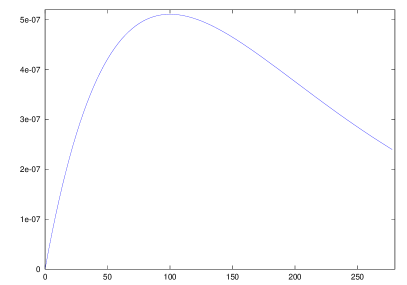
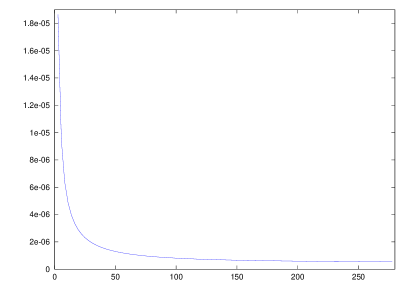
Figure 5: Absolute and relative error for discrete approximation

3.2.2 Per-demand Failure Modeling

The correct modeling of a per demand failure mode is more complex. Not only the occurrence pattern, but also the modeling of the direct effect must be adapted to probabilistic modeling. The challenge is that the system which executes a demand and the failure automaton which indicates whether the demand succeeds or fails must take a step at the same time and the failure automaton is not allowed to take a transition if there is no demand, or else the computed probabilities are not correct.

For the occurrence pattern, a predicate demand is defined which indicates that there is a demand to the safety critical component. The per-demand failure automaton can only leave the state “no” if demand holds, see Fig. 6. The state “no” has two transitions, one loop which is active if there is either no demand $\neg$ demand or if there is a demand but the demand succeeds with probability $(1-p)$ ($p$ being the per-demand failure probability). The state “no” is only left with probability $p$ if demand holds.

Figure 6: Per-demand failure automaton

The integration of the direct effect of a per-demand failure into the system model is a bit more complicated. It is illustrated via the integration of the failure mode of the second arithmetic unit A2FailsActivate of the example in Sect. 2.2. At first, the predicate $activate$ which means the hot stand-by mode must be left, is used to define the demand as $demand:=activate$, i.e. the demand is the activation command for the secondary arithmetic unit. The activation can only fail if it is actually called, therefore it is modeled as a per-demand failure.

Now if the $demand$ holds, the failure automaton and the system can make a transition in parallel. Therefore the information whether the demand has been met is available after the transition has been taken. In order to get the timing correct, an additional state is introduced which represents either failure or success of the demand, depending on the state of the failure automaton.

For the example this can be seen in Fig. 7. The demand ($activate$) is possible in state $idle$. The original successor states of $idle$ were $sig$ if the demand was successful and $idle$ if the demand failed (see Fig. 3). For the probabilistic modeling the state $idle^{\prime}$ is added to represent a failed demand if at the same time the failure automaton is in state “yes” and a successful demand if the failure automaton is in state “no”. To preserve the original behavior of the system, the transitions of $idle$ and $sig$ must be added to the state $idle^{\prime}$ in conjunction with the predicates $in(idle)$ or $in(sig)$ which are defined as shown in Eq. (4) and (5).

$$in(idle) := state=idle\vee(state=idle^{\prime}\wedge failure=yes)$$ (4)

$$in(sig) := state=sig\vee(state=idle^{\prime}\wedge failure=no)$$ (5)

These predicates must then also be exported from the modules and be substituted in all other places where $state=idle$ or $state=sig$ appears (predicates for transitions, logic formulas etc.). If this is done, the observable behavior of the automaton is the same as the original failure effects modeling as defined in [34] and shown in Fig. 3 for the example, but with a correct modeling of the per-demand failure occurrence pattern and direct effect.

Figure 7: Transformation for per demand failure mode

3.2.3 General Per-Demand failure integration

The last section illustrated the integration of a per-demand failure mode for the given example. In general, this integration requires first to define what constitutes a “demand” for a given failure mode. This typically results in a state formula, which divides the set of all states (of the system) in states where there is a demand for the functionality of the component and those where there is no demand. Now, for all states $s\in S$ where a demand to a component is exists, let $A_{s}\subseteq S$ be the set of direct successors states if there was a successful demand and $B_{s}\subseteq S$ if it was unsuccessful, i.e.

$A_{s}:=\{a\in S|\exists$ transition from $s$ to $a$ with activation condition $demand\wedge failure=no$}

$B_{s}:=\{b\in S|\exists$ transition from $s$ to $b$ with activation condition $demand\wedge\neg failure=no$}

There can also be successor states of $s$ that are not in $A_{s}\cup B_{s}$, the successors if there was no demand (where $demand$ as in the definition of $A_{s}$ and $B_{s}$ does not hold) to the safety critical system. These states do not play any role in the following construction, but are one of the main causes that the construction is required. The reason is that if there is no demand and therefore the successor of $s$ is not in $A_{s}\cup B_{s}$, the failure automaton is not allowed to make a transition.

Let $T_{A_{s}}:=\{$ Transitions from $s$ to $d$ with $d\in A$}, $\Phi_{A_{s}}:=\{\phi|\;\phi\wedge failure=no$ is activation condition of any $t\in T_{A}\}$, and define $T_{B_{s}}$ and $\Phi_{B_{s}}$ analogously, let $T:=T_{A_{s}}\cup T_{B_{s}}$, $\Phi:=\Phi_{A_{s}}\cup\Phi_{B_{s}}$. As the model is required to be deterministic, $\forall\phi_{i},\phi_{j}\in\Phi_{A},i\neq j:\phi_{i}\wedge\phi_{j}=false$ holds, the same holds for $\Phi_{B}$. Now demand can be defined as $(state=s)\wedge\bigvee_{\phi\in\Phi}\phi$.

To integrate a per demand failure, the following steps must be executed for each automaton $M$ in which direct effects of a failure mode are modeled, resulting in an automaton $M^{\prime}$:

1. Define $M^{\prime}$ with the same states as $M$. All transitions but those starting from state $s$ and going to states in $A\cup B$ are kept.

2. Define a new state $s^{\prime}$ in $M^{\prime}$ which represents being in any state $d\in A_{s}\cup B_{s}$, add a transition from $s$ to $s^{\prime}$ where the activation condition is demand

3. Define a decide automaton which is used to specify which state $d\in A_{S}\cup B_{s}$, the state machine $M^{\prime}$ really has, the set of possible states for the decision automaton is $A_{s}\times B_{s}\cup\{undef\}$.

4. Add failure probabilities to the corresponding failure automaton as in Fig. 4.

5. For each transition from $d\in A_{s}\cup B_{s}$ to a successor $d^{\prime}$ with activation condition $\psi$ add a transition from $s^{\prime}$ to $d^{\prime}$ in $M^{\prime}$ with the activation condition $\psi\wedge in(d)$

6. In the decide automaton, let $undef$ be the initial state and add a to transition to a state $d=[a,b]\in A_{s}\times B_{s}$ if the transition from $s$ to $a$ is activated if $failure=no$ holds and the transition from $s$ to $b$ is activated if $\neg failure=no$ holds.

7. Add the corresponding transitions also between the states $d\in A\times B$ of the decide automaton if a demand is possible in two consecutive time steps

This construction allows the failure automaton to make a transition from no iff demand holds, $M^{\prime}$ makes a transition from $s$ to $s^{\prime}$ and the respective decide automaton makes a transition to one of its states. For each of the original successor states $d\in A_{s}\cup B_{s}$, the predicate $M^{\prime}=d$ is not enough to characterize the fact that $M^{\prime}$ is in state $d$. Therefore the predicate $in(d)$ as shown in equation (6) and (7) is introduced and replaces the occurrences of $M^{\prime}=d,d\in A_{s}\cup B_{s}$, for $d\in A_{s}$ as shown in Eq. (6) and for $d\in B_{s}$ as shown in Eq. (7).

$$in(d) := M^{\prime}=d\vee(M^{\prime}=s^{\prime}\wedge decide=[s,d]\wedge failure=no)$$ (6)

$$in(d) := M^{\prime}=d\vee(M^{\prime}=s^{\prime}\wedge decide=[s,d]\wedge\neg failure=no)$$ (7)

Because of the determinism and the requirements of a total transition relation, the successor state of $s$ is always well-defined, as for each label predicate $l\in\mathcal{P}($atomic predicates of $\phi\in\Phi_{A}\cup\Phi_{B}$) there is exactly one transition to a state if $failure=no$ and exactly one transition if $\neg failure=no$.

In the example of Sect. 3.2.2 the decide automaton has been omitted in order to illustrate the idea of per-demand failure mode integration without too much complexity. As $idle^{\prime}$ only represents two different states, and therefore the distinction using the $failure$ predicate is enough. But for more complex systems with several possible per-demand failures, the general construction using the additional decide automaton is necessary.

4 Quantitative Safety Analysis

The probabilistic models of Sect. 3 can now be used to compute the overall hazard probabilities of the system using probabilistic logics and probabilistic model checkers.

4.1 Probabilistic Model Checking

For discrete time probabilistic models, the probabilistic logic probabilistic computational tree logic (PCTL) is used. For continuous time model, continuous stochastic logic (CSL) is used. Their respective semantics can be found in [27, 19].

PCTL is a probabilistic variant of CTL. Instead of Kripke structures as in CTL model-checking, labeled Markov chains are the system model for PCTL model checking. Both are very similar, the main difference is that in Kripke structures there is either a transition between states or there is none. In labeled Markov chains there is either no transition between states or it has an assigned probability. PCTL formulas are of the form:

$$P_{\sim p}[\phi]\sim\in\{<,\leq,>,\geq\}$$

and assert that for the probability $P$ of the path formula $\phi$ the equation $P\sim p$ holds. This means (for example), for a given system the given formula $\phi$ holds with a probability $P$ and $P\leq p$. Intuitively this means, that the probability that $\phi$ holds on a system trace starting in the initial state is less than or equal to $p$. The other operators are defined analogously.

It is also possible to (automatically) calculate the probability directly. The according syntactic expression is: $P_{=?}[\phi]$. Instead of giving a result true or false, this returns the actual probability that the formula $\phi$ holds on a given system trace.

The path operator available in PCTL is the  U operator. “Globally (G)” and “Eventually (F)” operators can be derived from this operator ($G\phi:=\neg(true{\bf\,U\,}\neg\phi)$ and $F\phi:=(true{\bf\,U\,}\phi)$). Negation of a formula is formulated by using $P_{\leq 0}$. In order to compute the probability of the negation of a formula $\phi$, $1-P_{=?}[\phi]$ can be used. The existence of a trace on which $\phi$ holds can be checked with $P_{>0}[\phi]$.

The exact definitions of semantics and probability measures can be found in [27, 19]. Algorithms to check PCTL formulas can be found in [27]. Efficient model checking algorithms are implemented in tools like PRISM [26] or MRMC [23]. A comparison of the efficiency and memory usage of different probabilistic model checkers including stochastic simulation based model checkers using hypothesis testing can be found in [22].

4.2 Computation of Hazard Probabilities

PCTL proof obligations can then be used together with the probabilistic model to compute the precise probability that the hazard occurs, given the per-time failure rates and the per-demand failure probabilities of the failure modes.

The semantics for PCTL are defined for infinite system traces. This cannot be used to compute the hazard probability, as it would always be either 1 if the hazard can occur or 0 if the hazard cannot occur.

Instead, the analysis is conducted for a given time range. What is computed is the probability that the hazard occurs in $k$ time steps of length $\delta t$. To accomplish this, the bounded until temporal operator is used. If $\phi{\bf\,U\,}^{\leq k}\psi$ holds, then there exists a bound $j\leq k$, so that $\psi$ becomes true after no more that $j$ steps and $\phi$ is true for all time steps $i<j$. Using the bounded until operator, the occurrence probability of the hazard $H$ in time $t=k\delta t$ is computed via Eq. (8) which is basically the bounded PCTL DCCA formula of Def. 1 for an empty minimal critical set.

$$P_{k}(H):=P_{=?}[true{\bf\,U\,}^{\leq k}H]$$ (8)

It is important to note, that the direct analogon to the DCCA formula $\left(P_{k}(\Gamma):=P_{=?}[\overline{\Gamma}{\bf\,U\,}^{\leq k}H],\Gamma\neq\emptyset\right)$ does not compute the probability of the failure modes in the minimal critical set $\Gamma$ causing the hazard $H$. The reason is that $\overline{\Gamma}{\bf\,U\,}^{\leq k}H$ limits the set of traces to those where only those failure modes in $\Gamma$ can appear. This is adequate to analyze whether these failure modes are sufficient to cause $H$ as it is done with DCCA (which is a worst case analysis).

Nevertheless for probabilistic analysis the probability of all traces where $\Gamma$ is the cause of $H$ is important, i.e. also the traces where $\Gamma$ causes $H$ but other failure modes appear but without any direct effect on the occurrence of $H$. For example, if A2 fails transiently before the monitor fails and then A1 fails, the cause for “no signal output” is the minimal critical set {A1FailsSig, MonitorFails}. But the probability of the trace where A2FailsSig appears would not be considered, as $\overline{\Gamma}{\bf\,U\,}^{\leq k}H$ limits the traces to those where only A1FailsSig and MonitorFails appear.

Instead of pure DTMC models as shown here, it is also possible to use MDPs (Markov decision processes) which allow a non-deterministic choice between different distribution functions in a state. Instead of exact probabilities, MDP analysis allows for computation of minimal and maximal probabilities. For safety analysis, the maximal (worst case) probability of the hazard is of interest, as shown in Eq. 9.

$$Pmax_{k}(H):=Pmax_{=?}[true{\bf\,U\,}^{\leq k}H]$$ (9)

4.3 Quantitative Results

For the analysis of the example case study, all failure modes were modeled as per time failure modes with the exception of the per demand failure A2FailsActivate. The minimal critical sets are given in Sect. 2.3.

Assuming an error rate of $10^{-2}\frac{1}{h}$ for each per time failure mode and using a temporal resolution $\delta t=10ms$, this translates to a per-step failure probability of $p_{fail}=2.\overline{7}\cdot 10^{-8}$ for the per-time failure modes. For the failure mode “A2ActivateFails”, a per demand failure probability of $10^{-4}$ is assumed.

Using PRISM the computation of the hazard “no output delivered” can be computed for a for $k=360000$ (i.e. running time of 1h) using the probabilistic modeling as described in Sect. 3 The result is shown in Eq. 10. The analysis was conducted on an AMD64 3Ghz and needed ca. 140s to complete. In this case the dominant factor in the analysis time is the large number of iterations, as $k$ matrix multiplications are required. This can very likely be made much faster using new approaches for probabilistic model checking [8, 6].

$$P_{Quant}(H)=2.964375\cdot 10^{-17}$$ (10)

If a quantitative method based on the a-posteriori analysis of the qualitative results like FTA is used, the estimation of the actual hazard probability is either very pessimistic (if the dependency of the ordering is not considered) or it can get very complex. For example to increase the accuracy, the system model must be analyzed further and the dependencies of the effects of the various failure modes must be explored (the model is based on finite state machines and time passes if a state changes which can then be detected in the next time step). In addition, as many as possible of the possible occurrence patterns of the failure modes must be enumerated to enhance the result. On the other hand, the probabilistic analysis can do this automatically and is much less error prone than such an a-posteriori analysis of the model.

5 Related Work

Several approaches for quantitative safety analysis exist which rely mainly on the analysis of a previous qualitative analysis. This can be either fault tree analysis (FTA) [42] or methods to compute the critical failure combinations directly from a model. One example is DCCA [33], other methods relying on fault injection were developed in the ESACS project [11] like the FSAP/NuSMV-SA framework [10] or in the ISAAC project [4] were SCADE was used for modeling and safety analysis [3]. In order for the estimation of the global hazard probability, the “FTA-formula” is used (see Eq. (11)) which gives an upper bound for the hazard probability.

$$P(H)\leq\sum_{\Delta\in mcs}\prod_{\delta\in\Delta}P(\delta)$$ (11)

It is clear, that no ordering information is considered in this formula as it depends on all probabilities being independent, so the estimation can be very pessimistic. With dynamic fault trees (DFT) [40], ordering information and dependencies can be analyzed, they can partly be deduced from the models directly [9, 16] and can give more accurate results than FTA. Nevertheless it is still based on a-posteriori analysis of qualitative results with the corresponding disadvantages.

In the COMPASS project [12] the FSAP-NuSMV/SA [10] framework is combined with the MRMC [24] probabilistic model checker to allow for the analysis of systems for Aerospace applications specified in the SLIM [13] language, which is inspired by AADL [38, 39]. The hybrid behavior of the SLIM models and all internal transitions are removed by lumping and the resulting interactive Markov chain is analyzed with MRMC.

Another approach for probabilistic safety analysis is probabilistic failure modes and effects analysis (FMEA) [15] where per-time failure behavior is integrated into system models via failure injection. After then, FMEA tables are computed which are often used in industrial safety analysis processes.

Both these approaches use continuous Markov chains models (CTMC) and only use per-time failure mode modeling with failure rates. The semantically correct integration of per-demand failure mode into continuous time models is difficult at best and in general not possible (non-deterministic behavior may occur). But it would be very interesting to see how these methods, especially the SLIM modeling language can be used for synchronous parallel system and in discrete time models.

In the AVACS project [36], another model-based safety analysis approach based on statecharts was developed [7]. It also uses continuous time models, but an additional difference is, that the hazard probability is analyzed for each minimal cut set. As explained in Sect. 4.2, the probability for a given set to cause the hazard is not easy to compute. Therefore it is not done in [7], but an “importance analysis” is conducted, analyzing single critical combinations and rating them according to their contribution to the global hazard probability.

6 Conclusion and Future Work

We showed how model-based safety analysis can be conducted on extended system models with probabilistic failure behavior. Per-demand as well as per-time failure modes can be integrated and the overall probability of a hazard occurrence in a given time interval can be computed. This quantitative analysis is well applicable to synchronous parallel systems.

The method has been applied to much larger case studies with more than $10^{8}$ states and due to recent developments in the area of probabilistic model checking, e.g. using the GPU [8], parallel model checking [6], abstraction techniques [25, 5, 21] and also simulation based stochastic hypothesis testing [44] still larger systems will likely be analyzable in the future. Hypothesis testing is very interesting, as it allows to give probabilistic results with confidence intervals based on several simulation runs. Using it, probabilistic analysis can give reliable results even if complete model checking is not possible.

In any way, this model-based analysis can give insights into the properties of a safety critical system in the in early phases of the design, where the cost of redesign is lowest.

At the moment, a framework is developed which allows for both qualitative and quantitative analysis on the same model, automating the complex integration of per-demand failures as presented here. The given approximation of the continuous distribution and the time discretization worked well in the considered case studies. Nevertheless additional estimation of the accuracy of the results is aspired, depending on the temporal resolution and the discrete probabilities, especially for probabilistically modeled environment behavior other than failure modes. Very beneficial would be the direct integration into tools like Topcased [41] or SCADE, which requires additional work for the transformation from these into our framework. But the semantic proximity of the SCADE execution models and the already accomplished integration of DCCA into it [17] are evidence that this is possible.

References

- [1]
- [2] (2009). ISO/WD 26262: Road Vehicles-Functional Safety.
- [3] Parosh Aziz Abdulla, Johann Deneux, Gunnar Stalmarck, Herman Agren & Ove Akerlund (2004): Designing Safe, Reliable Systems using SCADE. In: Proceedings of ISOLA’04. Springer-Verlag.
- [4] O. Akerlund, P. Bieber, E. Boede, M. Bozzano, M. Bretschneider, C. Castel, A. Cavallo, M. Cifaldi, J. Gauthier, A. Griffault, O. Lisagor, A. Luedtke, S. Metge, C. Papadopoulos, T. Peikenkamp, L. Sagaspe, C. Seguin, H. Trivedi & L. Valacca (2006): ISAAC, a framework for integrated safety analysis of functional, geometrical and human aspects. In: Proceedings of ERTS 2006.
- [5] C. Baier, P. R. D’Argenio & M. Grosser (2005): Partial Order Reduction for Probabilistic Branching Time. In: Proceedings of the Third Workshop on Quantitative Aspects of Programming Languages (QAPL 2005), Edinburgh, Scotland, Electronic Notes in Theoretical Computer Science 153. Elsevier, pp. 97–116.
- [6] Jiri Barnat, Lubos Brim, Ivana Cerná, Milan Ceska & Jana Tumova (2008): ProbDiVinE-MC: Multi-core LTL Model Checker for Probabilistic Systems. In: QEST. pp. 77–78.
- [7] Eckard Böde, Thomas Peikenkamp, Jan Rakow & Samuel Wischmeyer (2008): Model Based Importance Analysis for Minimal Cut Sets. Reports of SFB/TR 14 AVACS 29, SFB/TR 14 AVACS. ISSN: 1860-9821.
- [8] D. Bosnacki, S. Edelkamp & D. Sulewski (2009): Efficient Probabilistic Model Checking on General Purpose Graphics Processors. In: Proc. 16th International SPIN Workshop, LNCS 5578. Springer, pp. 32–49.
- [9] M. Bozzano & A. Villafiorita (2003): Integrating Fault Tree Analysis with Event Ordering Information. In: Proceedings of ESREL’03. Balkema, pp. 247–254.
- [10] M. Bozzano & Adolfo Villafiorita (2003): Improving System Reliability via Model Checking: theFSAP/NuSMV-SA Safety Analysis Platform. In: Proceedings of SAFECOMP’03. Springer, pp. 49–62.
- [11] M. Bozzano et al. (2003): ESACS: An Integrated Methodology for Design and Safety Analysis of Complex Systems. In: Proceedings of European Safety and Reliability Conference (ESREL’03). Balkema publisher, Maastricht, The Netherlands, pp. 237–245.
- [12] Marco Bozzano, Alessandro Cimatti, Joost-Pieter Katoen, Viet Yen Nguyen, Thomas Noll & Marco Roveri (2009). COMPASS project webpage. http://compass.informatik.rwth-aachen.de/.
- [13] Marco Bozzano, Alessandro Cimatti, Joost-Pieter Katoen, Viet Yen Nguyen, Thomas Noll & Marco Roveri (2009): Model-Based Codesign of Critical Embedded Systems. In: 2nd International Workshop on Model Based Architecting and Construction of Embedded Systems. CEUR-WS.org, pp. 87–91.
- [14] E. Clarke, O. Grumberg & D. Peled (2000): Model Checking. MIT Press.
- [15] L. Grunske, R. Colvin & K. Winter (2007): Probabilistic Model-Checking Support for FMEA. In: Proc. 4th International Conference on Quantitative Evaluation of Systems (QEST’07).
- [16] M. Güdemann, F. Ortmeier & W. Reif (2008): Computing Ordered Minimal Critical Sets. In: E. Schnieder & G. Tarnai, editors: Proceedings of Formal Methods for Automation and Safety in Railway and Automotive Systems (FORMS/FORMAT).
- [17] Matthias Güdemann, Frank Ortmeier & Wolfgang Reif (2007): Using Deductive Cause Consequence Analysis (DCCA) with SCADE. In: Proceedings of SAFECOMP 2007. Springer LNCS 4680.
- [18] N. Halbwachs, P. Caspi, P. Raymond & D. Pilaud (1991): The synchronous data-flow programming language Lustre. Proceedings of the IEEE 79(9), pp. 1305–1320.
- [19] Hans Hansson & Bengt Jonsson (1994): A Logic for Reasoning about Time and Reliability. Formal Aspects of Computing 6, pp. 102–111.
- [20] Holger Hermanns, Joost-Pieter Katoen, Joachim Meyer-Kayser & Markus Siegle (2000): A Markov Chain Model Checker. In: TACAS ’00: Proceedings of the 6th International Conference on Tools and Algorithms for Construction and Analysis of Systems. Springer, London, UK, pp. 347–362.
- [21] Holger Hermanns, Björn Wachter & Lijun Zhang (2008): Probabilistic CEGAR. In: CAV ’08: Proceedings of the 20th international conference on Computer Aided Verification. Springer, Berlin, Heidelberg.
- [22] David N. Jansen, Joost-Pieter Katoen, Marcel Oldenkamp, Mariëlle Stoelinga & Ivan Zapreev (2007): How Fast and Fat Is Your Probabilistic Model Checker? In: Haifa Verification Conference, HVC’07, Springer.
- [23] J.-P. Katoen, M. Khattri & I. Zapreev (2005): A Markov Reward Model Checker. In: Quantitative Evaluation of Systems (QEST). IEEE Computer Society, Los Alamos, CA, USA, pp. 243–244.
- [24] J.-P. Katoen, M. Khattri & I. Zapreev (2005): A Markov reward model checker. In: 2nd Int. Conf. on Quantitative Evaluation of Systems, Turin, Italy. IEEE Computer Society, pp. 243–245.
- [25] Joost-Pieter Katoen, Tim Kemna, Ivan S. Zapreev & David N. Jansen (2007): Bisimulation Minimisation Mostly Speeds Up Probabilistic Model Checking. In: TACAS. pp. 87–101.
- [26] M. Kwiatkowska, G. Norman & D. Parker (2002): Probabilistic Symbolic Model Checking with PRISM: A Hybrid Approach. In: J.-P. Katoen & P. Stevens, editors: Proc. 8th International Conference on Tools and Algorithms for the Construction and Analysis of Systems (TACAS’02), LNCS 2280. Springer, pp. 52–66.
- [27] M. Kwiatkowska, G. Norman & D. Parker (2007): Stochastic Model Checking. In: M. Bernardo & J. Hillston, editors: Formal Methods for the Design of Computer, Communication and Software Systems: Performance Evaluation (SFM’07), LNCS (Tutorial Volume) 4486. Springer, pp. 220–270.
- [28] Peter B. Ladkin (2008). An Overview of IEC 61508 on EEPE Functional Safety.
- [29] Robin E. McDermott, Raymond J. Mikulak & Michael R. Beauregard (1996): The Basics of FMEA. Quality Resources.
- [30] K. L. McMillan (1990): Symbolic Model Checking. Kluwer Academic Publishers.
- [31] MOD0058 (1996): HAZOP studies on systems containing programmable electronics. UK Ministry of Defence.
- [32] F. Ortmeier, W. Reif & G. Schellhorn (2005): Formal safety analysis of a radio-based railroad crossing using Deductive Cause-Consequence Analysis (DCCA). In: Proceedings of 5th European Dependable Computing Conference EDCC, LNCS 3463. Springer.
- [33] F. Ortmeier, W. Reif & G. Schellhorn (2006): Deductive Cause-Consequence Analysis (DCCA). In: Proceedings of IFAC World Congress. Elsevier.
- [34] Frank Ortmeier, Matthias Güdemann & Wolfgang Reif (2007): Formal Failure Models. In: First IFAC Workshop on Dependable Control of Discrete Systems (DCDS 07). Elsevier.
- [35] T. Peikenkamp, E. Böde, I. Brückner, H. Spenke, M. Bretschneider & H.-J. Holberg (Toulouse, 2004): Model-based Safety Analysis of a Flap Control System. In: In Proceedings of the INCOSE 2004 – 14th Annual International Symposium.
- [36] AVACS Funding Proposal (2003): AVACS – Automatic Verification and Analysis of Complex Systems. Technical Report, University of Oldenburg.
- [37] RTCA (1992). DO-178B: Software Considerations in Airborne Systems and Equipment Certification.
- [38] SAE-AS5506 (2004).
- [39] SAE-AS5506/1 (2006). Volume 1, Annex E: Error Model Annex.
- [40] M. Čepin & B. Mavko (2002): A dynamic fault tree. Reliability Engineering & System Safety 75.
- [41] François Vernadat, Christian Percebois, Patrick Farail, Robertus Vingerhoeds, Alain Rossignol, Jean P. Talpin & David Chemouil (2006): The TOPCASED Project - A Toolkit in OPen-source for Critical Applications and SystEm Development. In: Data Systems In Aerospace (DASIA). European Space Agency (ESA Publications).
- [42] Dr. W. Vesley, Dr. Joanne Dugan, J. Fragole, J. Minarik II & J. Railsback (2002): Fault Tree Handbook with Aerospace Applications. NASA Office of Safety and Mission Assurance.
- [43] Martin Walker, Leonardo Bottaci & Yiannis Papadopoulos (2007): Compositional Temporal Fault Tree Analysis. In: SAFECOMP. pp. 106–119.
- [44] Håkan L. S. Younes (2005): S.: Ymer: A statistical model checker. In: Computer Aided Verification. Springer.