Stochastic Calculus of Wrapped Compartments

Abstract

The Calculus of Wrapped Compartments (CWC) is a variant of the Calculus of Looping Sequences (CLS). While keeping the same expressiveness, CWC strongly simplifies the development of automatic tools for the analysis of biological systems. The main simplification consists in the removal of the sequencing operator, thus lightening the formal treatment of the patterns to be matched in a term (whose complexity in CLS is strongly affected by the variables matching in the sequences).

We define a stochastic semantics for this new calculus. As an application we model the interaction between macrophages and apoptotic neutrophils and a mechanism of gene regulation in E.Coli.

1 Introduction

In computer science, several formalisms have been proposed for the description of the behaviour of biological systems. Automata-based models [2, 22] have the advantage of allowing the direct use of many verification tools such as model checkers. Rewrite systems [13, 25, 5] usually allow describing biological systems with a notation that can be easily understood by biologists. Compositionality allows studying the behaviour of a system componentwise. Both automata-like models and rewrite systems present, in general, problems from the point of view of compositionality, which, instead, is in general ensured by process calculi, included those commonly used to describe biological systems [26, 24, 9].

The Calculus of Looping Sequences [5] (CLS) has been introduced to describe microbiological systems, such as cellular pathways, and their evolution. The terms of the calculus are constructed by basic constituent elements and operators of sequencing, looping, containment and parallel composition. The looping operator allows tying up the ends of a sequence, thus creating a circular sequence which can represent a membrane. The presence of sequences and loops, however, makes more difficult to develop a correct and efficient implementation of the associated simulation tools. The main difficulties come from the complexity of the pattern matching algorithms which should take sequences (and all their subsequences) into account. Moreover, the use of sequences and sequence variables seems prone to subtle semantic ambiguities in rules definition.

In this paper we propose the Calculus of Wrapped Compartments (CWC for short), a variant of CLS suitable for efficient implementation. In CWC, starting from an alphabet of atomic elements, we build multisets of elements and compartments. We are able to localise elements by compartmentalisation and we allow to specify the structure of the compartment (e.g., detailing the elements of interest on a membrane). The evolution of the system is driven by a set of rewrite rules modelling the reactions of interest. The main difference with respect to CLS consists in removing the sequencing operator and using multisets (instead of ordered sequences) of atoms to represent membranes. Such a choice, while preserving the Turing completeness of the calculus, strongly simplifies the pattern matching algorithm and the underlying basic theory.

In our previous experience with biological models we realized that sequences were not used in many situations: cellular pathways are usually represented with a greater abstraction than the one which uses amino acids and nucleotides to depict proteins and genes - moreover representing the primary sequence of a protein without considering secondary and tertiary structure is seldom useful. CLS used looping sequences to represent membranes, but we believe that multisets of atomic elements are a more natural representation, which reflects the fluid mosaic model [28]. A similar approach is taken in the CLS+ model (see [6]), a variant of CLS in which the looping operator can be applied to a parallel composition of sequences.

We provide CWC with a stochastic operational semantics from which a continuous time Markov chain can be build. With respect to [4], in which a constant rate is associated to the rewrite rules, we allow a more flexible treatment of the dynamics. In particular, we associate a function to each rewrite rule according to which the rate of the transition can be computed depending on the initial and the target terms. We show how the law of mass action can be encoded in our stochastic semantics thus following the standard Gillespie’s approach [17].

Summary.

In Section 2 we introduce the new formalism and show its Turing completeness. In Section 3 we provide some guidelines for the modelling of common biological events. We give some detail on how the interaction between macrophages and apoptotic neutrophils, and a mechanism of gene regulation can be described in the new calculus. In Section 4 we present a stochastic semantics of the calculus. In Section 5, we report some simulations regarding the gene regulation mechanism introduced in Section 3. Finally, in Section 6 we draw some conclusions.

2 The Calculus of Wrapped Compartments

In this section we present the nondeterministic Calculus of Wrapped Compartments (CWC).

2.1 Terms and Structural Congruence

A term of the CWC calculus is intended to represent a biological system. A term is a sequence of simple terms. Simple terms, ranged over by $t$, $u$, $v$, $w$, are built by means of the compartment constructor, $(-\,\rfloor\,-)$, from a set $\mathcal{A}$ of atomic elements (atoms for short), ranged over by $a$, $b$, $c$, $d$. The syntax of simple terms is given at the top of Figure 1. We write $\overline{t}$ to denote a (possibly empty) sequence of simple terms $t_{1}\cdot\cdot\cdot t_{n}$. Similarly, with $\overline{a}$ we denote a (possibly empty) sequence of atoms. The set of simple terms will be denoted by $\mathcal{T}$. The set of terms (sequences of simple terms) and the set of sequences of atoms will be denoted by $\overline{\mathcal{T}}$ and $\overline{\mathcal{A}}$, respectively. Note that $\overline{\mathcal{A}}\subseteq\overline{\mathcal{T}}$.

A term $\overline{t}=t_{1}\cdot\cdot\cdot t_{n}$ should be understood as the multiset containing the simple terms $t_{1},\ldots,t_{n}$. Therefore, we introduce a relation of structural congruence, following a standard approach in process algebra. The CWC structural congruence is the least equivalence relation on terms satisfying the rules given at the bottom of Figure 1. From now on we will always consider terms modulo structural congruence. Then a simple term is either an atom or a compartment $(\overline{a}\,\rfloor\,\overline{t})$ consisting of a wrap (represented by the multiset of atoms $\overline{a}$) and a content (represented by the term $\overline{t}$). We write the empty multiset as $\bullet$ and denote the union of two multisets $\overline{u}$ and $\overline{v}$ as $\overline{u}\;\,\overline{v}$.

  
Simple terms syntax $\begin{array}[]{lcl}\\ t&\;\mathrel{\makebox[20.00003pt]{$::=$}}&a\!\quad\big{|}\quad\!(\overline{a}\,\rfloor\,\overline{t})\\ \\ \end{array}$
  
Structural congruence
$\begin{array}[]{l}\\ \overline{t}\;\,u\;\,w\;\,\overline{v}\equiv\overline{t}\;\,w\;\,u\;\,\overline{v}~{}~{}~{}~{}~{}~{}~{}~{}~{}~{}~{}~{}~{}~{}\mbox{ if }\;\overline{a}\equiv\overline{b}~{}~{}\text{and}~{}~{}\overline{t}\equiv\overline{u}~{}~{}\mbox{ then }~{}~{}(\overline{a}\,\rfloor\,\overline{t})\equiv(\overline{b}\,\rfloor\,\overline{u})\\ \\ \end{array}$  

Figure 1: CWC term syntax and structural congruence rules.

An example of term is $a\;\,b\;\,(c\;\,d\,\rfloor\,e\;\,f)$ representing a multiset consisting of two atoms $a$ and $b$ (for instance two molecules) and a compartment $(c\;\,d\,\rfloor\,e\;\,f)$ which, in turn, consists of a wrap (a membrane) with two atoms $c$ and $d$ (for instance, two proteins) on its surface, and containing the atoms $e$ (for instance, a molecule) and $f$ (for instance a DNA strand). See Figure 2 for some graphical representations.

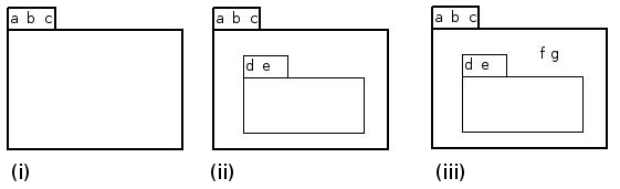
Figure 2: (i) represents $(a\;\,b\;\,c\,\rfloor\,\bullet)$; (ii) represents $(a\;\,b\;\,c\,\rfloor\,(d\;\,e\,\rfloor\,\bullet))$; (iii) represents $(a\;\,b\;\,c\,\rfloor\,(d\;\,e\,\rfloor\,\bullet)\;\,f\;\,g)$.

2.2 Systems and Reduction Semantics

Rewrite rules are defined as pairs of terms, in which the left term characterizes the portion of the system in which the event modelled by the rule can occur, and the right one describes how that portion of the system is changed by the event.

In order to formally define the rewriting semantics, we introduce the notion of open term (a term containing variables) and pattern (an open term that may be used as left part of a rewrite rule). In order to respect the syntax of terms, we distinguish between “wrap variables” which may occur only in compartment wraps (and can be replaced only by multisets of atoms) and “term variables” which may only occur in compartment contents or at top level (and can be replaced by arbitrary terms). Therefore, we assume a set of term variables, $\mathcal{V}_{\overline{\mathcal{T}}}$, ranged over by $X,Y,Z$, and a set of wrap variables, $\mathcal{V}_{\overline{\mathcal{A}}}$, ranged over by $x,y,z$. These two sets are disjoint. We denote by $\mathcal{V}$ the set of all variables $\mathcal{V}_{\overline{\mathcal{T}}}\cup\mathcal{V}_{\overline{\mathcal{A}}}$, and with $\rho$ any variable in $\mathcal{V}$.

Definition 2.1 (Open Terms and Patterns)

 

• Open terms are terms which may contain occurrences of wrap variables in compartment wraps and term variables in compartment contents or at top level. They can be seen as multisets of simple open terms. More formally, open terms, ranged over by $O$ and simple open terms, ranged over by $o$, are defined in the following way:

  $$\begin{array}[]{lcl}O&\mathrel{\makebox[20.00003pt]{$::=$}}&\overline{o}\\ o&\mathrel{\makebox[20.00003pt]{$::=$}}&a\quad\big{|}\quad X\quad\big{|}\quad(\overline{a}\;\,\overline{x}\,\rfloor\,\overline{o})\end{array}$$

• An open term is linear if each variable occurs at most once in it.

• Simple patterns, ranged over by $S$, are the linear open terms defined in the following way:

  $$S\; \;\mathrel{\makebox[20.00003pt]{$::=$}}\;t\quad\big{|}\quad(\overline{a}\;\,x\,\rfloor\,\overline{S}\;\,X)$$

  where $t$ is an element of $\mathcal{T}$, $\overline{a}$ is an element of $\overline{\mathcal{A}}$, $x$ is a variable in $\mathcal{V}_{\overline{\mathcal{A}}}$, $\overline{S}$ is a possibly empty multiset of simple patterns and $X$ is a variable in $\mathcal{V}_{\overline{\mathcal{T}}}$. We denote with $\mathcal{S}$ the set of simple patterns.

• Patterns, ranged over by $P$, are the linear open terms defined in the following way:

  $$P \;\mathrel{\makebox[20.00003pt]{$::=$}}\;S\;\,\overline{S}\;\,X$$

  where $S~{}\overline{S}$ is a nonempty multiset of simple patterns and $X$ is an element of $\mathcal{V}_{\overline{\mathcal{T}}}$. We denote with $\mathcal{P}$ the set of patterns.

An instantiation is a partial function $\sigma:\mathcal{V}\rightarrow\overline{\mathcal{T}}$. An instantiation must preserve the type of variables, thus for $X\in\mathcal{V}_{\overline{\mathcal{T}}}$ and $x\in\mathcal{V}_{\overline{\mathcal{A}}}$ we have $\sigma(X)\in\overline{\mathcal{T}}$ and $\sigma(x)\in\overline{\mathcal{A}}$, respectively. Given $O\in\mathcal{O}$, with $O\sigma$ we denote the term obtained by replacing each occurrence of each variable $\rho\in\mathcal{V}$ appearing in $O$ with the corresponding term $\sigma(\rho)$. With $\Sigma$ we denote the set of all the possible instantiations, and, given $O\in\mathcal{O}$, with $\textit{Var}(O)$ we denote the set of variables appearing in $O$. Now we can define rewrite rules.

Definition 2.2 (Rewrite Rules)

A rewrite rule is a pair of a pattern $P$ and an open term $O$, denoted with $P\!\mapsto\!O$, such that $\textit{Var}(O)\subseteq\textit{Var}(P)$.

A rewrite rule $P\!\mapsto\!O$ states that a term $P\sigma$, obtained by instantiating variables in $P$ by some instantiation function $\sigma$, can be transformed into the term $O\sigma$. A set of rewrite rules define a notion of reduction between terms of CWC which are intended to represent the (nondeterministic) behaviour of the represented system.

Definition 2.3

A CWC system over a set $\mathcal{A}$ of atoms is represented by a set $\mathcal{F}_{\mathcal{A}}$ ($\mathcal{F}$ for short when $\mathcal{A}$ is understood) of rewrite rules over $\mathcal{A}$.

We define the semantics of CWC as a transition system in which states correspond to terms and transitions correspond to rule applications. To this aim we need to define the notion of contexts (i.e. terms containing a hole).

Definition 2.4 (Contexts)

Contexts $C$ are defined as:

$$C\;\mathrel{\makebox[20.00003pt]{$::=$}}\;\square\quad\big{|}\quad(\overline{a}\,\rfloor\,C)\;\,\overline{t}$$

where $\overline{a}\in\overline{\mathcal{A}}$ and $\overline{t}\in\overline{\mathcal{T}}$. The context $\square$ is called the empty context. We denote with $\mathcal{C}$ the set of contexts.

By definition, every context contains a single hole $\square$. Let us assume $C,C^{\prime}\in\mathcal{C}$. With $C[\overline{t}]$ we denote the term obtained by replacing $\square$ with $\overline{t}$ in $C$; with $C[C^{\prime}]$ we denote context composition, whose result is the context obtained by replacing $\square$ with $C^{\prime}$ in $C$. For example, given $C=(a\;\,b\,\rfloor\,\square)\;\,i\;\,l$, $C^{\prime}=(c\;\,d\,\rfloor\,\square)\;\,g\;\,h$ and $\overline{t}=e\;\,f$, we get $C[C^{\prime}[\overline{t}]]=(a\;\,b\,\rfloor\,(c\;\,d\,\rfloor\,e\;\,f)\;\,g\;\,h)\;\,i\;\,l$. Note that context holes take the place either of the whole term or of the whole content of a compartment. This allows to make context unambiguous in the following sense. Let’s extend the notion of subset (denoted as usual as $\subseteq$) between terms interpreted as multisets.

Proposition 2.5 (Uniqueness)

For any term $\overline{t}$ if the term $\overline{u}$ occurs in $\overline{t}$ within a compartment content or at top level, then there are, modulo $\equiv$, a unique context $C$ and a unique term $\overline{t^{\prime}}$ such that $\overline{t}=C[\overline{t^{\prime}}]$ and $\overline{u}\subseteq\overline{t^{\prime}}$.

Given a CWC system $\mathcal{F}$ the associated notion of reduction is then defined in the following way.

Definition 2.6 (Reduction)

Given a CWC system $\mathcal{F}$, the $\mathcal{F}$-reduction relation between terms of CWC is defined by the following rule:

$$\frac{P\mapsto O\in\mathcal{F}\qquad\sigma\in\Sigma\qquad\overline{t}=P\sigma\qquad\overline{u}=O\sigma\qquad C\in\mathcal{C}}{C[\,\overline{t}\,]\mapsto_{\mathcal{F}}C[\overline{u}]}$$

closed under structural congruence, i.e.:

$$\overline{u}\equiv\overline{u^{\prime}}~{}~{}\text{and}~{}~{}\overline{u^{\prime}}\mapsto_{\mathcal{F}}\overline{v^{\prime}}~{}~{}\text{and}~{}~{}\overline{v^{\prime}}\equiv\overline{v}~{}~{}~{}~{}~{}\Rightarrow~{}~{}~{}~{}~{}\overline{u}\mapsto_{\mathcal{F}}\overline{v}$$

We will write simply $\mapsto$ instead of $\mapsto_{\mathcal{F}}$ when $\mathcal{F}$ is understood.

Remark 2.7

 

• Taken a pattern $P=S\;\,\overline{S}\;\,X$ (representing the reactants of the reaction that will be simulated) the crucial point for determining an application of $P$ to the whole biological ambient $\overline{t}$ is the choice of the occurrences of simple terms matching with $S\;\,\overline{S}$ (determining the compartment in which this reaction will take place). By Proposition 2.5 and the linearity condition both the context $C$ (such that $\overline{t}\equiv C[\overline{t^{\prime}}]$) and the term replacing $X$ (the part of $\overline{t^{\prime}}$ that does not match $S\;\,\overline{S}$) are uniquely determined. This will play a role in the implementation of the stochastic calculus.

• There can be, in general, many different substitution such that $P\sigma\equiv\overline{t}$ but not all of them produce the same term $O\sigma$ (modulo $\equiv$). This is not particularly relevant for the case of qualitative systems but we will need to take it into account in the stochastic formulation.

Notation 2.8

 

• We write $S\;\,\overline{S}\Rightarrow O$ as short for $S\;\,\overline{S}\;\,X\mapsto O\;\,X$, where the variable $X$ does not occur in $\textit{Var}(S\;\,\overline{S})\cup\textit{Var}(O)$.

• We write $a\;\,\overline{a}\rightarrow\overline{b}$ as short for the rewrite rule $(a\;\,\overline{a}\;\,x\,\rfloor\,Y)\;\,Z\mapsto(\overline{b}\;\,x\,\rfloor\,Y)\;\,Z$, where the variables $x,Y,Z$ are distinct.

The CWC is Turing Complete. In the following we sketch how Turing Machines can be simulated by CWC models.

Theorem 2.9 (Turing Completeness)

The class of CWC models is Turing complete.

Proof: (Sketch). A Turing machine $T$ over an alphabet $\Sigma\cup\{\sharp\}$ (where $\sharp$ represent the blank) with a set $Q$ of states can be simulated by a system $\mathcal{F}_{T}$ of CWC in the following way.
Take $\overline{\mathcal{A}}=Q\cup\Sigma\cup\{\sharp,l,r\}$, where $l$ and $r$ are special symbols to represent the left and right ends of the tape. The tape of the Turing machine can be represented by a sequence of nested compartments whose wraps consist of a single atom (representing a symbol of the tape). The content of each compartment defined in this way represents a right suffix of the written portion of the tape, while the atom on the wrap represents its initial (w.r.t. the suffix) symbol. In each term representing a tape there is exactly one compartment which contains a state (the present state). For example, the term $(l\,\rfloor\,(a\,\rfloor\,q~{}(b\,\rfloor\,(r\,\rfloor\,\bullet))))$ represents the configuration in which the tape is $...\sharp,a,b,\sharp....$ (the remaining positions are blank), the machine is in state $q$ and the head is positioned on $b$. Rewrite rules are then used to model the machine evolution. We can define rules creating new blanks when needed (at the tape ends) to mimic a possibly infinite tape. For instance a transition $(q,b)\rightarrow(q^{\prime},c,right)$ (meaning that in state $q$ with a $b$ on the head the machine goes in state $q^{\prime}$ writing $c$ on the tape and moving the head right) is represented by the rules:

$$\begin{array}[]{ll}(1)&q~{}(b~{}y\,\rfloor\,(x\,\rfloor\,Z)~{}Y)~{}X\mapsto(c~{}y\,\rfloor\,q^{\prime}~{}(x\,\rfloor\,Z)~{}Y)~{}X\\ (2)&q~{}(b~{}y\,\rfloor\,(r\,\rfloor\,Z)~{}Y)~{}X\mapsto(c~{}y\,\rfloor\,q^{\prime}~{}(\sharp\,\rfloor\,(r\,\rfloor\,Z))~{}Y)~{}X\end{array}$$

The second rule represents the case that b is the rightmost non blank symbol and so a new blank must be introduced in the simulation. By construction, the system $\mathcal{F}_{T}$ correctly represents the behaviour of $T$. $\Box$

3 Modelling Guidelines

Biomolecular Entity	CWM term
Elementary object (genes, domains, etc…)	Atoms
Molecular population	Term multiset
Membrane	Atom multiset

Table 1: Guidelines for the abstraction of biomolecular entities into CWC.

Biomolecular Event	Examples of CWC Rewrite Rules
State change	$a\Rightarrow b$
Complexation	$a\;\,b\Rightarrow c$
Decomplexation	$c\Rightarrow a\;\,b$
Catalysis	$c\;\,S\;\,\overline{S}\Rightarrow c\;\,O$ where $S\;\,\overline{S}\Rightarrow O$ is the catalyzed event
State change on membrane	$a\rightarrow b$
Complexation	$a\;\,b\rightarrow c$
on membrane	$a\;\,(b\;\,x\,\rfloor\,X)\Rightarrow(c\;\,x\,\rfloor\,X)$
	$(b\;\,x\,\rfloor\,a\;\,X)\Rightarrow(c\;\,x\,\rfloor\,X)$
Decomplexation	$c\rightarrow a\;\,b$
on membrane	$(c\;\,x\,\rfloor\,X)\Rightarrow a\;\,(b\;\,x\,\rfloor\,X)$
	$(c\;\,x\,\rfloor\,X)\Rightarrow(b\;\,x\,\rfloor\,a\;\,X)$
Catalysis on membrane	$c\;\,a\;\,\overline{a}\rightarrow c\;\,\overline{b}$ where $a\;\,\overline{a}\rightarrow\overline{b}$ is the catalyzed event
Membrane crossing	$a\;\,(x\,\rfloor\,X)\Rightarrow(x\,\rfloor\,a\;\,X)$
	$(x\,\rfloor\,a\;\,X)\Rightarrow a\;\,(x\,\rfloor\,X)$
Catalyzed	$a\;\,(b\;\,x\,\rfloor\,X)\Rightarrow(b\;\,x\,\rfloor\,a\;\,X)$
membrane crossing	$(b\;\,x\,\rfloor\,a\;\,X)\Rightarrow a\;\,(b\;\,x\,\rfloor\,X)$
Membrane joining	$a\;\,(x\,\rfloor\,X)\Rightarrow(a\;\,x\,\rfloor\,X)$
	$(x\,\rfloor\,a\;\,X)\Rightarrow(a\;\,x\,\rfloor\,X)$
Catalyzed	$a\;\,(b\;\,x\,\rfloor\,X)\Rightarrow(a\;\,b\;\,x\,\rfloor\,X)$
membrane joining	$(b\;\,x\,\rfloor\,a\;\,X)\Rightarrow(a\;\,b\;\,x\,\rfloor\,X)$
	$(x\,\rfloor\,a\;\,b\;\,X)\Rightarrow(a\;\,x\,\rfloor\,b\;\,X)$
Membrane fusion	$(a\;\,x\,\rfloor\,X)\;\,(b\;\,y\,\rfloor\,Y)\Rightarrow(a\;\,x\;\,b\;\,y\,\rfloor\,X\;\,Y)$
Vesicle dynamics	$(x\,\rfloor\,X\;\,(a\;\,y\,\rfloor\,Y))\Rightarrow Y\;\,(a\;\,y\;\,x\,\rfloor\,X)$

Table 2: Guidelines for the abstraction of biomolecular events into CWC.

In this section we will give some explanations and general hints about how CWC could be used to represent the behaviour of various biological systems.

In rewrite systems, such as CWC, entities are usually represented by terms of the rewrite system, and events by rewrite rules. We have already introduced the biological interpretation of our terms in Section 2.1. Here we will go deeper and describe the most straightforward abstraction that can be used to define terms and rules.

First of all, we should select the biomolecular entities of interest. Since we want to describe cells, we consider molecular populations and membranes. Molecular populations are groups of molecules that are in the same compartment of the cells and inside them. As we have said before, molecules can be of many types: we classify them as proteins, chemical moieties and other molecules.

Membranes are considered as elementary objects: we do not describe them at the level of the phospholipids they are made of. The only interesting properties of a membrane are that it may have a content (hence, create a compartment) and that in its phospholipid bilayer various proteins are embedded, which act for example as transporters and receptors. Since membranes are represented as multisets of the embedded structures, we are modelling a fluid mosaic in which the membranes become similar to a two-dimensional liquid where molecules can diffuse more or less freely [28].

Now, we select the biomolecular events of interest. The simplest kind of event is the change of state of an elementary object. Then, there are interactions between molecules: in particular complexation, decomplexation and catalysis. Interactions could take place between simple molecules, depicted as single symbols, or between membranes and molecules: for example a molecule may cross or join a membrane. Finally, there are also interactions between membranes: in this case there may be many kinds of interactions (fusion, vesicle dynamics, etc…).

The guidelines for the abstraction of biomolecular entities and events into CWC are given in Table 1 and Table 2, respectively. Biomolecular events are associated with rewrite rules. In the table we give some examples of rewrite rules for different kinds of events. The list has not the ambition of being complete but to give some general hints on rules definition.

3.1 Modelling Examples

We will now present two examples of possible CWC simulations, in order to testify that our calculus is able to express a broad range of biological situations even if the possibility to represent sequences, which is a computational burden, is removed from its syntax.

Macrophages.

All the biological problems involving cell interactions are feasible. One could for example represent macrophages and their interaction with the apoptotic cells: in order to “clean up” the remains of death cells they have to recognize them amongst the alive ones and then remove them by a process called phagocytosis, which consists in the internalization of the death cell in a membrane compartment, called phagosome. The phagosome inside the macrophage will then join another membrane compartment called the lysosome in order to start the degradation of the ingested cellular components.

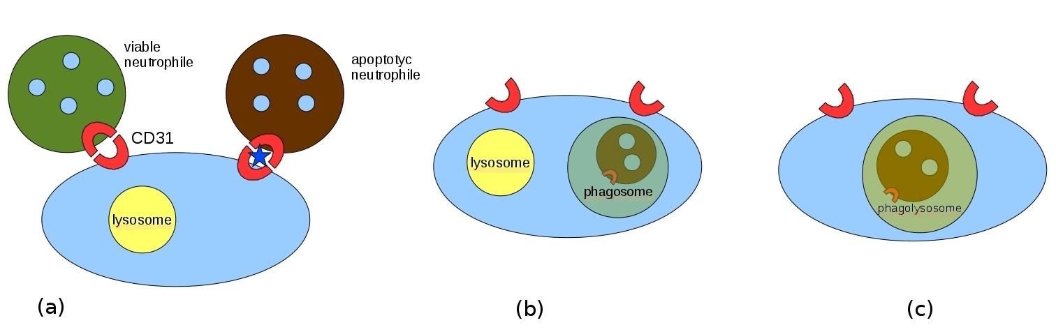
Figure 3: Neutrophils phagocytosis: a) a macrophage distinguishes between apoptotic and living neutrophils, b) the death neutrophile is “eaten” and embedded in a phagosome, c) the phagosome fuses with a lysosome.

To give the rules that could represent this process in CWC we decided to concentrate on the removal of neutrophils that have undergone apoptosis: removing them before their membrane collapses is crucial because they contain some lytic enzymes that, if released in the organism, would lead to tissue damages [15, 12]. The mechanism which mediates the recognition of apoptotic neutrophils is not perfectly clear but we decided to reproduce the one described in [29, 8] which suggest that neutrophils and macrophages interact via CD31 and that somehow the CD31 of vial neutrophils is capable of “escaping” the phagocytosis.

We will represent a macrophage with a lysosome and a CD31 exposed on its membrane in this way (where M is a marker to distinguish macrophages from other cells and $lyso$ represents a lysosome containing some lytic enzymes):

$$(\mbox{CD31}\;\,\mbox{M}\,\rfloor\,(lyso\,\rfloor\,lyticEnz)\;\,innerM)$$

A living neutrophile (where N is a marker for neutrophils and V indicates that this is a viable neutrophile) is represented by:

$$(\mbox{CD31}\;\,\mbox{V}\;\,\mbox{N}\,\rfloor\,innerL)$$

An apoptotic one (where A indicates its apoptotic state) is represented by:

$$(\mbox{CD31}\;\,\mbox{A}\;\,\mbox{N}\,\rfloor\,innerA)$$

where $innerM$, $innerL$ and $innerA$ denote the internal material of a macrophage, a living neutrophile and an apoptotic one, respectively.

Now a fairly simple set of rules is sufficient to represent the whole process.

The binding of a neutrophile and a macrophage mediated by their CD31 molecules is represented by encapsulating the interacting cells within a new compartment wrapped with the marker I:

$$(\mbox{CD31}\;\,\mbox{M}\;\,x\,\rfloor\,X)\;\,(\mbox{CD31}\;\,\mbox{N}\;\,y\,\rfloor\,Y)\Rightarrow(\mbox{I}\,\rfloor\,(\mbox{CD31}\;\,\mbox{M}\;\,x\,\rfloor\,X)\;\,(\mbox{CD31}\;\,\mbox{N}\;\,y\,\rfloor\,Y))$$

After the contact the viable neutrophils are released:

$$(\mbox{I}\;\,z\,\rfloor\,(\mbox{CD31}\;\,\mbox{M}\;\,x\,\rfloor\,X)\;\,(\mbox{CD31}\;\,\mbox{N}\;\,\mbox{V}\;\,y\,\rfloor\,Y)\;\,Z)\Rightarrow(\mbox{CD31}\;\,\mbox{M}\;\,x\,\rfloor\,X)\;\,(\mbox{CD31}\;\,\mbox{N}\;\,\mbox{V}\;\,y\,\rfloor\,Y)$$

While the apoptotic ones are phagocyted ($phago$ represents the phagosome which contains the phagocyted neutrophile):

$$(\mbox{I}\;\,z\,\rfloor\,(\mbox{CD31}\;\,\mbox{M}\;\,x\,\rfloor\,X)\;\,(\mbox{CD31}\;\,\mbox{N}\;\,\mbox{A}\;\,y\,\rfloor\,Y)\;\,Z)\Rightarrow(\mbox{CD31}\;\,\mbox{M}\;\,x\,\rfloor\,(phago\,\rfloor\,(\mbox{CD31}\;\,\mbox{N}\;\,\mbox{A}\;\,y\,\rfloor\,Y))\;\,X)$$

The phagosome can join the lysosome to start hydrolysis ($phagolyso$ represents the phagolysosome derived from the fusion):

$$(lyso\;\,x\,\rfloor\,lyticEnz\;\,X)\;\,(phago\;\,z\,\rfloor\,(\mbox{CD31}\;\,\mbox{N}\;\,\mbox{A}\;\,y\,\rfloor\,Y)\;\,Z)\Rightarrow(phagolyso\;\,x\;\,z\,\rfloor\,(\mbox{CD31}\;\,\mbox{N}\;\,\mbox{A}\;\,y\,\rfloor\,Y)\;\,lyticEnz\;\,X\;\,Z)$$

This should show that interactions involving cells of the immune system can be represented in CWC with little effort at different levels of detail: modelling some aspects of the complex network that drives immunological defence could be useful to study many human pathologies and involved processes, like in this example about inflammation and how it stops.

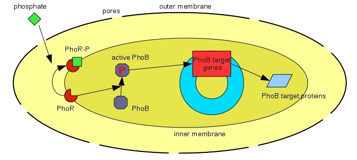
Figure 4: The Pho regulation system.

Phosphate regulation.

Switching to a completely different field we would like to describe a mechanism of gene regulation fairly well defined in E.Coli and other bacteria, which is based on a two component system: (i) the sensor, which can react to changes in the environment and interact with the other component; (ii) the response regulator, which is capable of determining, when activated by the sensor, the reactions necessary to cope with the new environmental conditions. This schema is common to drive gene regulation in bacteria: the activated response regulator will act as a transcriptional activator.

We will model the system related to environmental phosphate concentration, where the sensor is a transmembrane protein located on the inner membrane of the bacteria, called PhoR, and the response regulator is a cytoplasmatic protein which can be activated by phosphorylation and is called PhoB. Environmental phosphate will freely diffuse in the periplasmic space (between the two bacterial membranes) thanks to the outer membrane pores and there it will bind to PhoR. When bound by phosphate PhoR will be silent, while it shows a kinase activity on PhoB when it is unbound; therefore low levels of phosphate will leave many PhoR unbound and able to activate PhoB, while high levels will lead to a smaller fraction of transmembrane unbound PhoR and thus to little activation of PhoB. When phosphorylated, PhoB activates the transcription of many genes aimed at helping the bacteria survive in low phosphate conditions [21]. These mechanisms have been recently described as related to the pathogenic potential [16] of some bacteria and therefore studying them could also have some importance in medicine.

We will now present the set of rules needed to model this regulation system; in the following we will refer to the outer membrane pores as $pore$, to phosphate as $Pi$, to the phosphate bound and unbound PhoR as $PhoR$ and $PhoRP$, to the inactive and active PhoB as $PhoB$ and $PhoBP$, to its target genes as $PhoGenes$ and to the proteins that they encode as $PhoProt$.

We may represent an E.Coli with the following CWC term:

$$(pore\,\rfloor\,(\overline{PhoR}\;\,\overline{PhoRP}\,\rfloor\,\overline{PhoB}\;\,\overline{PhoBP}\;\,PhoGenes))$$

where, here, a sequence $\overline{PhoR}$ represents a multiset of $PhoR$ atoms (similar for the other atoms). Two rules describe the phosphate diffusion in the periplasmic space:

$$Pi\;\,(pore\;\,x\,\rfloor\,X)\Rightarrow(pore\;\,x\,\rfloor\,Pi\;\,X)$$

$$(pore\;\,x\,\rfloor\,Pi\;\,X)\Rightarrow Pi\;\,(pore\;\,x\,\rfloor\,X)$$

Two rules for the PhoR phosphate binding:

$$Pi\;\,(PhoR\;\,x\,\rfloor\,X)\Rightarrow(PhoRP\;\,x\,\rfloor\,X)$$

$$(PhoRP\;\,x\,\rfloor\,X)\Rightarrow Pi\;\,(PhoR\;\,x\,\rfloor\,X)$$

PhoB phosphorylation:

$$(PhoR\;\,x\,\rfloor\,PhoB\;\,X)\Rightarrow(PhoR\;\,x\,\rfloor\,PhoBP\;\,X)$$

High level rules that represent the translation and traduction to proteins of the PhoB target genes and these proteins degradation:

$$PhoBP\;\,PhoGenes\Rightarrow PhoBP\;\,PhoGenes\;\,PhoProt$$

$$PhoProt\Rightarrow\bullet$$

One last rule represents the bound form of PhoR phosphatase activity on PhoBP [10], which is a negative regulating loop of the whole mechanism:

$$(PhoRP\;\,x\,\rfloor\,PhoBP\;\,X)\Rightarrow(PhoRP\;\,x\,\rfloor\,PhoB\;\,X)$$

In Section 5 we will give some details about simulations of this model.

4 The Stochastic Calculus of Wrapped Compartments

In order to make the formal framework suitable to model quantitative aspects of biological systems we must associate to each rule a numerical parameter (the rule rate) which determines (in a stochastic sense) the time spent between two successive interactions and the frequency with which each interaction will take place in order to represent faithfully the system evolution. The operational semantics will be defined by incorporating the rule rates in a stochastic framework along the lines of the one presented by Gillespie in [17]. The same approach has been incorporated, for example, in other simulators as the ones for the stochastic $\pi$-calculus [23, 24].

In this framework the rule rate is used as the parameter of an exponential distribution modelling the time spent between two occurrences of the considered chemical reaction. The use of exponential distributions to represent the (stochastic) time spent between two occurrences of chemical reactions allows describing the system as a Continuous Time Markov Chain (CTMC), and consequently allows verifying properties of the described system analytically and by means of stochastic model checkers.

The basic choice for determining the rule rate of a reaction (suggested also by Gillespie’s algorithm) is to obtain it by multiplying the kinetic constant of the reaction by the number of possible combinations of reactants that may occur in the system, representing in this way the law of mass action.

In our calculus we will represent a reaction rate as a function of the context in which the reaction takes place. This allows to tailor the reaction rates on the specific characteristics of the system, as for instance when representing nonlinear reactions as it happens for Michaelis–Menten kinetics. The standard mass action rate can be describes as a particular choice of the rate function (see below). A similar approach is used in [14] to model reactions with inhibitors and catalysers in a single rule.

Obviously some care must be taken in the choice of the rate function: for instance it must be complete (defined on the domain of the application) and nonnegative. This properties are enjoyed by the function representing the law of mass action.

Definition 4.1

A stochastic rewrite rule is a triple $(P,R,f)$, denoted $P\stackrel{{\scriptstyle f}}{{\longmapsto}}R$, where $(P,R)$ is a rewrite rule and $f:\overline{\mathcal{T}}\times\overline{\mathcal{T}}\rightarrow\mathbb{R}^{\geq 0}$ is the rate function associated to the rule.

We can then define, as in Definition 2.6, the “stochastic” reduction relation for CWC. In this case, we must also take into account that, by Remark 2.7, different instantiations that allow the l.h.s. $P$ of a rule to match a term $\overline{t}$ can produce different outcomes which could determine different rates. This is shown in Example 4.2. So, in the definition of the rate function, we must also take into account the term produced by the reaction after the application of the rule.

Example 4.2

Consider the rewrite rule $a\;\,(b\;\,x\,\rfloor\,X)\stackrel{{\scriptstyle f}}{{\longmapsto}}(a\;\,b\;\,x\,\rfloor\,X)$ modelling a catalyzed membrane joining. In this case, the initial term $a\;\,(b\;\,b\,\rfloor\,c)\;\,(b\,\rfloor\,c)$ results in two different terms depending on which membrane will be joined by the element $a$; namely $(a\;\,b\;\,b\,\rfloor\,c)\;\,(b\,\rfloor\,c)$ and $(b\;\,b\,\rfloor\,c)\;\,(a\;\,b\,\rfloor\,c)$. The application of the rule, moreover, should take into account that the first case is catalyzed by the presence of two elements $b$ on the membrane, while the second one has only one catalyzer.

A Stochastic CWC systems $\mathcal{R}_{\mathcal{A}}$ ($\mathcal{R}$ for short) can be defined as in Definition 2.6 from a set $\mathcal{R}$ of stochastic reduction rules over $\mathcal{A}$.

Definition 4.3 (Stochastic Reduction)

Given a stochastic CWC system $\mathcal{R}$, the induced stochastic reduction relation between terms of CWC is defined by the following rule:

$$\frac{P\stackrel{{\scriptstyle f}}{{\longmapsto}}O\in\mathcal{R}\qquad\sigma\in\Sigma\qquad\overline{t}=P\sigma\qquad\overline{u}=O\sigma\qquad C\in\mathcal{C}}{C[\overline{t}]\stackrel{{\scriptstyle f(\overline{t},\overline{u})}}{{\longmapsto}}_{\mathcal{R}}C[\overline{u}]}$$

We will write simply $\stackrel{{\scriptstyle f}}{{\longmapsto}}$ instead of $\stackrel{{\scriptstyle f}}{{\longmapsto}}_{\mathcal{R}}$ when $\mathcal{R}$ is understood.

Chemical–like Reactions.

To define the “canonical” function that represents the law of mass action the application rate of a reduction rule should depend on the kinetic constant of the reaction and the number of possible reactants in the considered compartment in which the reaction will take place. Following an approach similar to that of [4, 18], this can be obtained counting the number of different ways in which the rule representing a reaction can be applied in the considered context producing the same outcome. In our setting, however, we can formalize the canonical function in a simpler way.

To this aim we need a few definitions. Assume to have an infinite set of labels (e.g. the natural numbers) that can be attached to the atomic elements in $\mathcal{A}$ to create, for each $a\in\mathcal{A}$ an infinite set of distinguished versions $a_{1},a_{2},a_{3},...$ of the element. If $a_{i}$ is a labelled atom, we write $a=|a_{i}|$ for the support of $a_{i}$.

Definition 4.4

 

• A labelled term of CWC is a term in which some labelled atomic element can occur.

• A complete labelled term is a term in which all atomic elements are labelled and no two labelled atoms having the same support have the same label.

• If $\overline{t}$ is a labelled term, its erasure $|\overline{t}|$ is the term obtained from $\overline{t}$ by erasing all the labels.

Labels can be applied also to atoms occurring in open terms, but no label can be associated to a variable.

If $\overline{t}$ is a labelled (possibly open) term a labeling $\overline{t^{+}}$ of $\overline{t}$ is obtained by assigning labels to the non labelled atoms of $\overline{t}$ such that $\overline{t^{+}}$ is a completely labelled term. For example, taking $\overline{t}=a_{1}~{}a~{}a_{3}~{}b$ a possible labeling of $\overline{t}$ is $\overline{t^{+}}=a_{1}~{}a_{2}~{}a_{3}~{}b_{1}$.

Given a reduction rule $P\stackrel{{\scriptstyle f}}{{\longmapsto}}O$ and terms $\overline{t},\overline{u}$ such that for some instantiation $\sigma$ it holds $P\sigma\equiv\overline{t}$ and $O\sigma\equiv\overline{u}$, we define the canonical rate function $f(\overline{t},\overline{u})$ by the following steps:

1. take any completely labeled version $\overline{t^{+}}$ of $\overline{t}$;

2. let $n$ be the number of distinct instantiations of variables with completely labeled terms such that $P^{\prime}\sigma\equiv\overline{t^{+}}$, for some labeling $P^{\prime}$ of $P$, and $|R\sigma|\equiv\overline{u}$;

3. define the function $f$ as $f(\overline{t},\overline{u})=k\cdot n$ where $k$ is the kinetic constant of the associated reaction.

We denote with $f^{can}_{k}$ the function obtained in this way to compute the evolution rate following the law of mass action with kinetic constant $k$.

Note that since the labels of the atomic elements are all different, by Proposition 2.5 and Remark 2.7 (i) each instantiation $\sigma$ such that $P^{\prime}\sigma\equiv\overline{t^{+}}$ corresponds to a distinct combination of the elements that determine the reaction described by the rule $P\stackrel{{\scriptstyle}}{{\longmapsto}}O$. So the number $n$ of substitutions defined in point 2. corresponds exactly to the number of possible distinct reactants for the considered reaction.

This number can often be calculated in a rather simple way. For instance in a rule $X\;a\;b~{}\stackrel{{\scriptstyle}}{{\longmapsto}}~{}X\;c$ each instantiation of $X$ that matches any term containing at least one $a$ and one $b$ corresponds exactly to a pair of occurrences of $a$ and $b$ (the ones not included in the variable’s instantiation). So the total number of distinct instantiations of $X$ (i.e. of possible reactants) is given by the product of the number of occurrences of $a$ times the number of occurrences of $b$.

Example 4.5

Consider the completely labeled term $\overline{t^{+}}=a_{1}~{}a_{2}~{}a_{3}~{}b_{1}$ defined above and the qualitative reduction rule $a~{}a~{}X\mapsto a~{}c~{}X$. The l.h.s. of the rule can be matched by the instantiations $X=a_{1}~{}b_{1}$, $X=a_{2},b_{1}$ and $X=a_{3}~{}b_{1}$. In the first case, the match is obtained by taking $P^{\prime}=a_{2}~{}a_{3}~{}X$ and so on. So, we have that $f^{can}_{k}(a~{}a~{}a~{}b,~{}a~{}a~{}c~{}b)=3\cdot k$ where $k$ is the kinetic constant of the reaction.

Example 4.6

Consider again the term $\overline{t}=a\;\,(b\;\,b\,\rfloor\,c)\;\,(b\,\rfloor\,c)$ and the rewrite rule $a\;\,(b\;\,x\,\rfloor\,X)\stackrel{{\scriptstyle f}}{{\longmapsto}}(a\;\,b\;\,x\,\rfloor\,X)$ described in Example 4.2. If the function $f$ is defined as the canonical function $f^{can}_{k}$, we get $\overline{t}\stackrel{{\scriptstyle 2\cdot k}}{{\longmapsto}}(a\;\,b\;\,b\,\rfloor\,c)\;\,(b\,\rfloor\,c)$ and $\overline{t}\stackrel{{\scriptstyle 1\cdot k}}{{\longmapsto}}(b\;\,b\,\rfloor\,c)\;\,(a\;\,b\,\rfloor\,c)$.

Remark 4.7

Note that the canonical function $f^{can}$ has the same meaning of the function $\mathcal{O}$ defined in [4].

5 An application

We used a prototype simulator for CWC to run some simulations for the Pho regulation system described in Section 3.1. In figure 5) we use $\stackrel{{\scriptstyle k}}{{\Rightarrow}}$ to indicate that we use the canonical function with kinetic constant k. The rates here are chosen manually following these considerations: diffusion of phosphate across the outer membrane pores has the same speed in both directions, PhoRP phosphatase activity is slow with respect to its kinase activity in the unbound form, both these mechanism are slower than the simpler binding and unbinding of phosphate to PhoR and the rules that describe translation and traduction and protein degradation should be rather slow.

$$Pi\;\,(pore\;\,x\,\rfloor\,X)\stackrel{{\scriptstyle 0.1}}{{\Rightarrow}}(pore\;\,x\,\rfloor\,Pi\;\,X)$$

$$(pore\;\,x\,\rfloor\,Pi\;\,X)\stackrel{{\scriptstyle 0.1}}{{\Rightarrow}}Pi\;\,(pore\;\,x\,\rfloor\,X)$$

$$Pi\;\,(PhoR\;\,x\,\rfloor\,X)\stackrel{{\scriptstyle 0.01}}{{\Rightarrow}}(PhoRP\;\,x\,\rfloor\,X)$$

$$(PhoRP\;\,x\,\rfloor\,X)\stackrel{{\scriptstyle 0.005}}{{\Rightarrow}}Pi\;\,(PhoR\;\,x\,\rfloor\,X)$$

$$(PhoR\;\,x\,\rfloor\,PhoB\;\,X)\stackrel{{\scriptstyle 0.001}}{{\Rightarrow}}(PhoR\;\,x\,\rfloor\,PhoBP\;\,X)$$

$$PhoBP\;\,PhoGenes\stackrel{{\scriptstyle 0.0001}}{{\Rightarrow}}PhoBP\;\,PhoGenes\;\,PhoProt$$

$$PhoProt\stackrel{{\scriptstyle 0.00008}}{{\Rightarrow}}\bullet$$

$$(PhoRP\;\,x\,\rfloor\,PhoBP\;\,X)\stackrel{{\scriptstyle 0.0001}}{{\Rightarrow}}(PhoRP\;\,x\,\rfloor\,PhoB\;\,X)$$

Figure 5: Stochastic rules for the phosphate regulation mechanism.

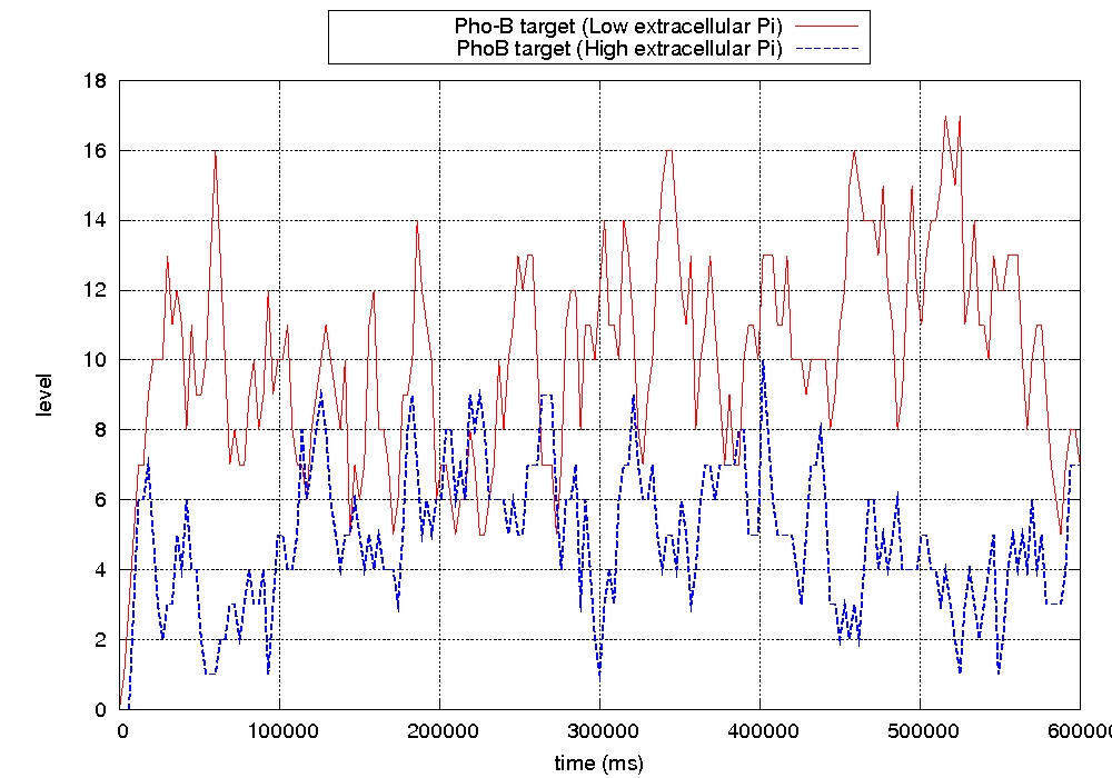
Figure 6: Levels of PhoB target proteins over time with different extracellular phosphate levels.

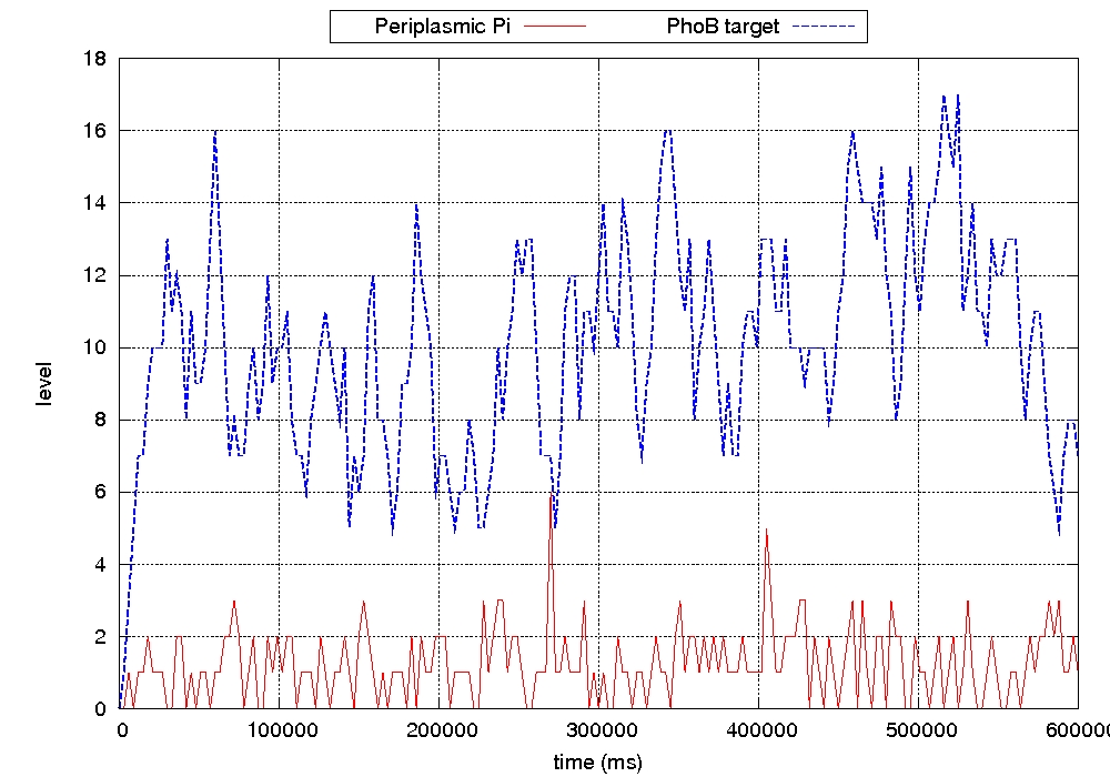
Figure 7: Levels of PhoB target proteins and periplasmic phosphate in the low extracellular phosphate conditions.

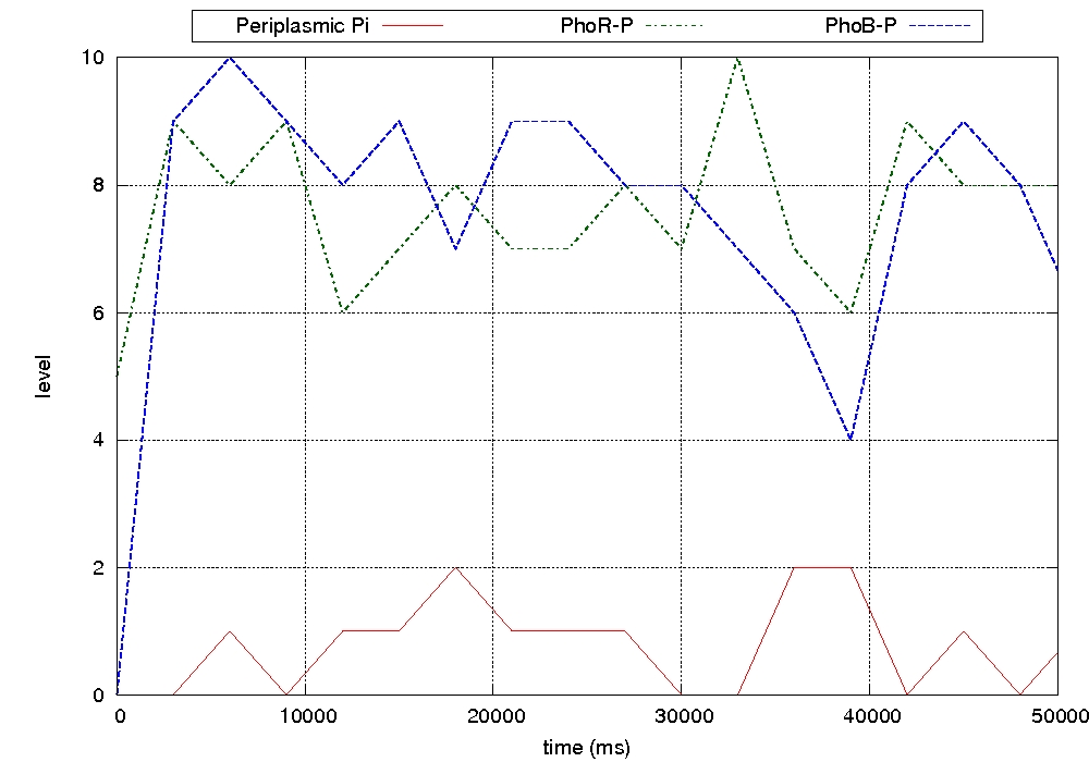
Figure 8: Levels of phosphorilated PhoB and phosphate bound PhoR in the low extracellular phosphate conditions.

We performed two simulations: both of them started with 10 PhoB, 5 PhoR, 5 PhoRP and a PhoGenes element in a single bacterial cell. To reflect high and low extracellular phosphate we started with 20 and 5 extracellular Pi, respectively. In Figure 6 we show the comparison of the PhoProt levels obtained in these simulations: as expected in the low phosphate condition the average level of the PhoB target proteins is higher. Figure 7 shows the relation between PhoProt levels and periplasmic phosphate for the low phosphate simulation: oscillations in the protein levels are in sync with the levels of periplasmic phosphate: when the latter increases the former decreases and viceversa. Figure 8 shows the beginning of the same simulation but focuses on the relationships between PhoRP, PhoPB and periplasmic phosphate: PhoRP levels follows with a little delay the phophate ones, while PhoBP shows a clearly specular behaviour with respect to PhoRP, as expected.

In the future we will like to compare the results of these simulations with available experimental data [3].

6 Conclusions

As we have seen, CWC allows to model cellular interaction, localisation and membrane structures. Other formalisms were developed to describe membrane systems. Among them we cite Brane Calculi [9] and P-Systems [25].

CWC can describe situations that cannot be easily captured by the above mentioned formalisms, which consider membranes as atomic objects. Representing the membrane structure as a multiset of the elements of interest allows the definition of different functionalities depending on the type and the number of elements on the membrane itself.

From a qualitative point of view, our calculus is essentially a variant of CLS [5], while, from a quantitative point of view, the possibility to model the speed of reactions using functions instead of constant rates makes the CWC stochastic semantics more general with respect to the one of SCLS [4]. In this sense, CWC stochastic semantics is more similar to the one in [14].

The current simulator for CWC is implemented in OCaml (see [1]). Since we do not need to analyse sequence structures and variables, the pattern matching algorithm has been simplified with respect to the simulator for SCLS described in [27].

We are also considering to enrich our analysis framework by taking into account statistical model checking as done in [7] for stochastic CLS models, and with techniques to approximate the value of unknown kinetics in the stile of [19, 20, 11].

References

- [1] M. Aldinucci, M. Coppo, F. Damiani, M. Drocco, E. Giovannetti, E. Grassi, and A. Troina. SCWC-bio-simulator. Dipartimento di Informatica, Università di Torino, 2010. http://scwc-sim.sourceforge.net/.
- [2] R. Alur, C. Belta, and F. Ivancic. Hybrid modeling and simulation of biomolecular networks. In HSCC, volume 2034 of LNCS, pages 19–32. Springer, 2001.
- [3] JH. Baek, YJ. Kang, and SY. Lee. Transcript and protein level analyses of the interactions among phob, phor, phou and crec in response to phosphate starvation in escherichia coli. FEMS Microbiol Lett., 277:254–259, 2007.
- [4] R. Barbuti, A. Maggiolo-Schettini, P. Milazzo, P. Tiberi, and A. Troina. Stochastic calculus of looping sequences for the modelling and simulation of cellular pathways. Transactions on Computational Systems Biology, IX:86–113, 2008.
- [5] R. Barbuti, A. Maggiolo-Schettini, P. Milazzo, and A. Troina. A calculus of looping sequences for modelling microbiological systems. Fundam. Inform., 72(1-3):21–35, 2006.
- [6] Roberto Barbuti, Andrea Maggiolo-Schettini, Paolo Milazzo, and Angelo Troina. The calculus of looping sequences for modeling biological membranes. In Workshop on Membrane Computing, volume 4860 of Lecture Notes in Computer Science, pages 54–76. Springer, 2007.
- [7] T. A. Basuki, A. Cerone, and P. Milazzo. Translating stochastic cls into maude. Electr. Notes Theor. Comput. Sci., 227:37–58, 2009.
- [8] S. Brown, I. Heinisch, E. Ross, K. Shaw, CD. Buckley, and J. Savill. Apoptosis disables CD31-mediated cell detachment from phagocytes promoting binding and engulfment. Nature, 418:200–203, 2002.
- [9] L. Cardelli. Brane calculi. In CMSB, volume 3082 of LNCS, pages 257–278. Springer, 2005.
- [10] DO. Carmany, K. Hollingsworth, and WR. McCleary. Genetic and biochemical studies of phosphatase activity of phor. J Bacteriol., 185:1112–1115, 2003.
- [11] A. Coletta, R. Gori, and F. Levi. Approximating probabilistic behaviors of biological systems using abstract interpretation. Electr. Notes Theor. Comput. Sci., 229(1):165–182, 2009.
- [12] G. Cox, J. Crossley, and Z. Xing. Macrophage engulfment of apoptotic neutrophils contributes to the resolution of acute pulmonary inflammation in vivo. Am J Respir Cell Mol Biol., 12:232–237, 1995.
- [13] V. Danos and C. Laneve. Formal molecular biology. Theor. Comput. Sci., 325(1):69–110, 2004.
- [14] M. Dezani-Ciancaglini, P. Giannini, and A. Troina. A type system for a stochastic cls. In MeCBIC, volume 11 of EPTCS, pages 91–106, 2009.
- [15] B. Fadeel and VE. Kagan. Apoptosis and macrophage clearance of neutrophils: regulation by reactive oxygen species. Redox Rep., 8:143–150, 2003.
- [16] GM. Ferreira and B. Spira. The pst operon of enteropathogenic escherichia coli enhances bacterial adherence to epithelial cells. Microbiology, 154:2025–2036, 2008.
- [17] D. Gillespie. Exact stochastic simulation of coupled chemical reactions. J. Phys. Chem., 81:2340–2361, 1977.
- [18] J. Krivine, R. Milner, and A. Troina. Stochastic bigraphs. Electron. Notes Theor. Comput. Sci., 218:73–96, 2008.
- [19] R. Lanotte, A. Maggiolo-Schettini, and A. Troina. Decidability results for parametric probabilistic transition systems with an application to security. In SEFM’04, pages 114–121. IEEE Computer Society, 2004.
- [20] R. Lanotte, A. Maggiolo-Schettini, and A. Troina. Parametric probabilistic transition systems for system design and analysis. Formal Asp. Comput., 19(1):93–109, 2007.
- [21] H. Lodish, A. Berk, L.S. Zipursky, P. Matsudaira, D. Baltimore, and J. Darnell. Many Bacterial Responses Are Controlled by Two-Component Regulatory Systems Molecular Cell Biology. W.H. Freeman, 2000.
- [22] H. Matsuno, A. Doi, M. Nagasaki, and S. Miyano. Hybrid petri net representation of gene regulatory network. In Prooceedings of Pacific Symposium on Biocomputing, pages 341–352. World Scientific Press, 2000.
- [23] C. Priami. Stochastic pi-calculus. Comput. J., 38(7):578–589, 1995.
- [24] C. Priami, A. Regev, E. Y. Shapiro, and W. Silverman. Application of a stochastic name-passing calculus to representation and simulation of molecular processes. Inf. Process. Lett., 80(1):25–31, 2001.
- [25] G. Pǎun. Membrane computing. An introduction. Springer, 2002.
- [26] A. Regev and E. Shapiro. Cells as computation. Nature, 419:343, 2002.
- [27] G. Scatena. Development of a stochastic simulator for biological systems based on the calculus of looping sequences. Master’s thesis, University of Pisa, 2007.
- [28] SJ. Singer and GL. Nicolson. The fluid mosaic model of the structure of cell membranes. Science, 175:720–731, 1972.
- [29] EF. Vernon-Wilson, F. Auradé, L. Tian, IC. Rowe, MJ. Shipston, J. Savill, and SB. Brown. CD31 delays phagocyte membrane repolarization to promote efficient binding of apoptotic cells. J Leukoc Biol., 82:1278–1288, 1995.