G30.79 FIR 10: A gravitationally bound infalling high-Mass star forming clump

Abstract

Context. The process of high-mass star formation is still shrouded in controversy. Models are still tentative and current observations are just beginning to probe the densest inner regions of giant molecular clouds.

Aims. The study of high-mass star formation requires the observation and analysis of high density gas. This can be achieved by the detection of emission from higher rotational transitions of molecules in the sub-millimeter. Here, we studied the high-mass clump G30.79 FIR 10 by observing molecular emission in the 345 GHz band. The goal is to understand the gravitational state of this clump, considering turbulence and magnetic fields, and to study the kinematics of dense gas.

Methods. We approached this region by mapping the spatial distribution of HCO${}^{+}(J=4\rightarrow 3)$, H¹³CO${}^{+}(J=4\rightarrow 3)$, CS$(J=7\rightarrow 6)$, ¹²CO$(J=3\rightarrow 2)$, and ¹³CO$(J=3\rightarrow 2)$ molecular emission by using the ASTE telescope and by observing the ¹²C¹⁸O$(J=3\rightarrow 2)$, HCN$(J=4\rightarrow 3)$, and H¹³CN$(J=4\rightarrow 3)$ molecular transitions with the APEX telescope.

Results. Infalling motions were detected and modeled toward this source. A mean infall velocity of 0.5 km s^-1with an infall mass rate of $5\times 10^{-3}$ M_⊙/yr was obtained. Also, a previously estimated value for the magnetic field strength in the plane of the sky was refined to be 855 $\mu$G which we used to calculate a mass-to-magnetic flux ratio, $\lambda=1.9$, or super-critical. The virial mass from turbulent motions was also calculated finding M${}_{\mathrm{vir}}=563$ M_☉, which gives a ratio of M_submm/M_vir=5.9. Both values strongly suggest that this clump must be in a state of gravitational collapse. Additionally, we estimated the HCO⁺ abundance, obtaining $X$(HCO⁺)= 2.4$\times 10^{-10}$.

1 Introduction

It is well known that massive stars ($\gtrsim$10 M_⊙) form in giant molecular clouds (GMCs), the largest molecular gas and dust complexes in our galaxy. The amount of gas involved in this process is several orders of magnitude larger than in the low-mass star formation scenario, which significantly increases the uncertainties that makes its study difficult. In contrast to the low-mass star formation case, where theory and observations have established clear evolutionary steps (McKee & Ostriker, 2007), there are no well defined stages for the evolution of proto-massive stars. Presently, two different mechanisms are proposed as the dominant process involved in the formation of massive stars. One mechanism is the coalescence of small fragments (Bonnell et al., 1998; Stahler et al., 2000; Bonnell et al., 2004). The other is accretion directly onto a massive protostellar object, which is supported by accumulating evidence for disks around proto-massive stars (Beuther & Sridharan, 2007; McKee & Ostriker, 2007).

The rate of formation of massive stars can be up to several orders of magnitude lower than low-mass stars, and they appear to be born in clusters. The process is highly energetic and dynamic, a massive star will quickly perturb and ionize its surrounding medium, which makes its study quite challenging (Wood & Churchwell, 1989; Hoare et al., 2007). Therefore, it is crucial to probe the densest regions in high massive star forming clumps to understand their physical and chemical conditions. In this regard, high rotational levels from molecules emitting in the sub-millimeter windows are the ideal tracers to go for. The combination of optically thick and optically thin isotopomers of the same molecular species can be used to infer physical properties from star formation sites.

The magnetic field is likely the least known physical parameter in star formation. While its presence seems to be ubiquitous within the ISM, with strengths ranging from a few $\mu$G to mG (Crutcher et al., 1999), there are surprisingly few observations. Moreover, while it is still unclear what role is played by the magnetic field in the formation of low-mass stars, the degree of uncertainty is even higher for high-mass star formation owing to the lack of observations. However, we can say with certainty that magnetic fields have been observed towards high-mass star forming regions (Cortes & Crutcher, 2006; Girart et al., 2009). Therefore, it is important to incorporate it as a relevant physical parameter in observations and models of high-mass start formation.

In this paper we present a multi-line study of the high-mass star forming region G30.79 FIR 10 The aim of this paper is to understand the gravitational state of this clump as well as to study the kinematics of the dense gas. We also use previous inteferometric observations of polarized dust emission to include information about the magnetic field toward this region. The paper is organized as follows, Sect. 1 is the introduction, Sect. 2 presents the source, Sect. 3 the observational procedure. In Sect. 4 we present the results, while in Sect. 5 we discuss the abundance of HCO⁺. The kinematics of the gas is studied in Sect. 5, where we present evidence for infall motions and discuss the likelihood of outflows. Additionally, we refined a previous estimation of the magnetic field strength in the plane of the sky for this source (Cortes & Crutcher, 2006), and use it to evaluate the gravitational state of this clump. Finally, Sect. 6 presents the summary and conclusions.

2 The source

G30.79 FIR 10 (hereafter G30.79) is a massive molecular complex located within the W 43 region. It involves an HII region-molecular cloud complex near $l=31^{\circ},b=0^{\circ}$, with several far-infrared sources, of which G30.79 is the most massive and densest component. Figure 1 presents an overview of our observations superposed over the 350 $\mu$m continuum map from Motte et al. (2003). Liszt (1995) observed G30.79 in HCO⁺ and ¹³CO  concluding that the presence of several rings and shells in the dense molecular gas was a disturbance product of star formation. Vallée & Bastien (2000) observed the dust continuum emission in this source at 760 $\mu$m using JCMT. They found linear polarization of about 1.9% with a position angle (P.A.) of 160^∘. Mooney et al. (1995) observed this source at 1.3 mm using the IRAM 30 m telescope, detecting a total flux density of 13.6 Jy; their wide field map shows the clump and the extended HII region in the G30.79 complex. H₂O masers have been observed toward this region (Cesaroni et al., 1988), which are within a half arc-second of the peak in the Mooney et al. (1995) map. Additionally, Ellingsen (2007) detected 6.7 GHz methanol masers in the proximity of G30.79, which is considered to be a signature for massive star formation. No centimeter radio-continuum emission seems to be associated with FIR 10, suggesting that the source could be in an early stage of evolution. However, the maser emission already indicates that star formation has started and outflows may be present. Motte et al. (2003) mapped the W43 main complex in dust continuum emission at 1.3 mm and 350 $\mu$m with the IRAM 30 m and CSO telescopes, respectively. They also mapped the HCO⁺ $J=3\rightarrow 2$ line and measured H¹³CO⁺ $J=3\rightarrow 2$ towards prominent dust maxima. One of the maxima, W43-MM1, corresponds to G30.79 and is the compact fragment we observed with ASTE. Motte et al. (2003) found $V_{\mathrm{lsr}}=98.8$ km s^-1, $\Delta v=5.9$ km s^-1 (from H¹³CO⁺), T${}_{\textnormal{dust}}\sim 19$ K, M$\sim 3600$ M_☉, and $n(\textnormal{H}_{2})\sim 8.8\times 10^{6}$ cm^-3. They estimated the virial mass to be M_vir$\sim$1000 M_⊙, suggesting that this compact fragment should be in a state of gravitational collapse unless there are other sources of support in addition to kinetic energy. Cortes & Crutcher (2006) mapped G30.79 in dust polarized emission at 1.3 mm using the BIMA interferometer founding a polarization pattern, which suggests an hour-glass morphology for the field. They also estimated the magnetic field strength in the plane of the sky to be $\sim$1.7 mG, which gave a statistically corrected mass-to-magnetic flux ratio of 0.9 or critical, where by critical we mean the equilibrium value between self-gravitation and magnetic field support for the cloud.

3 Observations

3.1 ASTE observations

G30.79 FIR 10 was observed during September 2006 using the Atacama Sub-millimeter Telescope Experiment (ASTE) from the National Astronomical Observatory of Japan (NAOJ) (Kohno, 2005). The telescope is located at Pampa la bola in the Chilean Andes plateau reserve for Astronomical research at 4900 meters of altitude. ASTE is a 10 m diameter antenna equipped with a 345 GHz double side band SIS-mixer receiver. We simultaneously observed ¹²CO$(J=3\rightarrow 2)$ and HCO${}^{+}(J=4\rightarrow 3)$, CS$(J=7\rightarrow 6)$ and ¹³CO$(J=3\rightarrow 2)$, and H¹³CO${}^{+}(J=4\rightarrow 3)$ with a beam size of $\sim 22^{\prime\prime}$, and a velocity resolution of 0.1 km s^-1, setting the MAC (which is a XF-type digital spectro-correlator) to a bandwidth of 128 MHz. The pointing accuracy was in the order of 2^′′, with Uranus used as the pointing source. The observations were done by performing raster maps (position switching) with a grid spacing of $15^{\prime\prime}$ (see Table 1 for map sizes), operating the telescope remotely from the ASTE base in San Pedro de Atacama under good weather conditions (precipitable water vapor or PWV $<$ 1 mm). Our reference position was $(\alpha,\delta)=(18^{\mathrm{h}}47^{\mathrm{m}}46.9^{\mathrm{s}},-1^{\circ}54^{\prime}29.1^{\prime\prime})$ (J2000), which coincides with the peak dust emission reported by Mooney et al. (1995); Motte et al. (2003); Cortes & Crutcher (2006). Unfortunately, the off position used to subtract the continuum had emission in the ¹²CO$(J=3\rightarrow 2)$ line. However, only the ¹²CO line-wings were affected (see discussion below). The M17SW molecular complex was used as an intensity calibrator. All temperatures are presented as T${}_{\mathrm{mb}}=$T${}^{*}_{\mathrm{A}}/\eta_{\mathrm{mb}}$, where $\eta_{\mathrm{mb}}=0.71\pm 0.07$. Initial data reduction and calibration was done using the NEWSTAR package, and the calibrated data were later exported into our own software for analysis and plotting.

3.2 APEX observations

Observations were performed during the first week of August 2008 using the Swedish Heterodyne Facility Instrument (SHFI) mounted on the Atacama Pathfinder Experiment telescope (APEX) (Güsten et al., 2006), located at llano de Chajnantor in the Chilean Andes. We tuned SHFI at 329.3 GHz in order to detect the ¹²C¹⁸O$(J=3\rightarrow 2)$ molecular transition, to 354.5 GHz for HCN$(J=4\rightarrow 3)$, and to 345.3 for H¹³CN$(J=4\rightarrow 3)$. The spectrometer was set up to 8192 channels with a resolution of 0.1 km s^-1. The main beam efficiency is $\eta$=0.73$\pm$0.07 as measured by the APEX staff, with a pointing accuracy better than 2^′′ and a beam size of $19^{\prime\prime}$. Jupiter and R-Aql were used as intensity calibrators where the observations were calibrated by the usual chopper-wheel method. The observations were done in raster mode with spacings of $15^{\prime\prime}$ from the same reference position used for the ASTE observations. The initial data reduction was done with the GILDAS-CLASS reduction package and the final analysis with our own software tools.

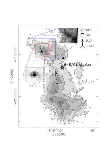
Figure 1: Overview of the G30.79 FIR 10 massive star forming region. The main panel represents the 350 $\mu$m continuum emission from Motte et al. (2003), Figure 1. Contours and grayscale are 12, 24, 48, 96, and 200 Jy beam^-1. The cluster of massive stars is indicated by the star symbol, while masers are indicated by the symbols presented at the upper right of the figure. Superimposed are our new ¹²CO$(J=3\rightarrow 2)$ and CS$(J=7\rightarrow 6)$ integrated velocity maps to show the extent of our observations.

Table 1: Line parameters

Line	Transition	Frequency	Observed Area	Tpeak	$\int$ T $dv$	Vpeak	$\Delta V$
		[GHz]	[arcsec2]	[K]	[K km s-1 ]	[km s-1 ]	[km s-1 ]
HCO+	$(J=4\rightarrow 3)$	356.7342880	$200^{\prime\prime}\times 150^{\prime\prime}$	5.7 $\pm 0.1$	42.6 $\pm 1.8$	94.8	8.4
H13CO+	$(J=4\rightarrow 3)$	346.9983381	$90^{\prime\prime}\times 90^{\prime\prime}$	1.2 $\pm 0.02$	5.5 $\pm 0.6$	98.1	3.0
HCN	$(J=4\rightarrow 3)$	354.5054779	$200^{\prime\prime}\times 150^{\prime\prime}$	3.8 $\pm 0.1$	73.5 $\pm 13.8$	93.8	9.5
H13CN	$(J=4\rightarrow 3)$	345.3397750	$30^{\prime\prime}\times 30^{\prime\prime}$	1.4 $\pm 0.1$	14.8 $\pm 0.4$	99.1	4.8
CS	$(J=7\rightarrow 6)$	342.8828503	$90^{\prime\prime}\times 90^{\prime\prime}$	3.6 $\pm 0.2$	38.7 $\pm 0.9$	98.5	3.8
12C16O	$(J=3\rightarrow 2)$	345.7959899	$200^{\prime\prime}\times 150^{\prime\prime}$	16 $\pm 2.2$	317 $\pm 21.1$	98.8	9.6
13C16O	$(J=3\rightarrow 2)$	330.5879652	$90^{\prime\prime}\times 90^{\prime\prime}$	8.5 $\pm 1.2$	125 $\pm 7.6$	97.4	6.3
12C18O	$(J=3\rightarrow 2)$	329.3305525	$30^{\prime\prime}\times 30^{\prime\prime}$	3.1 $\pm 0.2$	42.9 $\pm 10.0$	98.8	4.7

Parameters for all molecular line observations. The values for T_peak and $\Delta V$ are calculated from Gaussian fits to the central pointing or $(18^{\mathrm{h}}47^{\mathrm{m}}46.9^{\mathrm{s}},-1^{\circ}54^{\prime}29.1^{\prime\prime})$. For HCN and HCO⁺, the V_peak was taken from Gaussian fits done to the most intense component, while the line-width corresponds to the whole line. For ¹²CO and ¹³CO the fit was done over the whole spectrum.

4 Results

4.1 ¹²CO, ¹³CO, and ¹²C¹⁸O $(J=3\rightarrow 2)$ results

The ¹²CO $(J=3\rightarrow 2)$ line was detected all over the sampled region, covering an area of $3.5^{\prime}\times 2.5^{\prime}$ around the peak from the dust emission at 1.3 mm (see Fig. 1) The velocity integrated emission map is presented in Fig. 2 where the ¹²CO emission was integrated over the complete available velocity range (43 to 154 km s^-1 ). The peak in the map corresponds to 317 K km s^-1 located at about $85^{\prime\prime}$ to the south-west from the reference position, while the peak at the reference position is 234 K km s^-1. Overall we see most of the emission clustered in a south-west to north-east elongated pattern, which is consistent with the morphology of the dust emission seen in the maps from Motte et al. (2003) and Mooney et al. (1995). However, the peak in our ¹²CO map does not coincide with the peak in dust emission (located at our reference position). Figure 3 shows velocity channel maps binned every 5 km s^-1 (or 50 channels) with a resolution of 5.4 km s^-1 for each map with respect to the original resolution of 0.1 km s^-1. The channel maps are presented in increasing velocity from 84 to 106 km s^-1  covering the most intense features in the ¹²CO emission. By examining Fig. 3, a velocity gradient from the south-west to north-east can be seen with each successive channel where the peaks in emission are at 89 and 95 km s^-1 and at almost opposite spatial locations. Particularly interesting is the intense emission seen at the south-west part of the map. According to Motte et al. (2003, see Fig. 3 and also our Fig. 1), the giant HII region produced by a Wolf-Rayet cluster of massive stars has not yet reached the G30.79 clump. However, the Mooney et al. (1995) maps put the HII region at an interface with the clump. Because we could not sample beyond 105^′′ west, we can only speculate about the nature of this intense ¹²CO$(J=3\rightarrow 2)$ emission and whether it is related to an interface between this clump and the H II region without further observations.

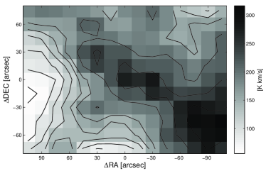
Figure 2: Velocity integrated ¹²CO$(J=3\rightarrow 2)$ map. The axis units are offsets in arc-seconds from the reference position $(18^{\mathrm{h}}47^{\mathrm{m}}46.9^{\mathrm{s}},-1^{\circ}54^{\prime}29.1^{\prime\prime})$ in J2000 coordinates. The gray-scale is in K km s^-1, while the contours are 3, 4, 5, 6, 7, 8, 10, 12, and 14$\sigma$ with $\sigma=20$ K km s^-1.

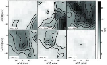
Figure 3: Channel maps for the ¹²CO line emission. Maps are shown as averages of 50 channels giving a velocity resolution of 5.4 km s^-1for each map. The average velocity in each plot is shown by the box in lower left corner of each map. Both $\Delta\alpha$ and $\Delta\delta$ are arc-second offset with respect to the reference position. The pixel scale is in K degrees and is normalized to the maximum and minimum values from all the maps set. The contours are from 3, 6, 9, 12, and 15$\sigma$, where $\sigma=0.9$ K. for all maps and calculated from a velocity range with no emission.

To study the velocity structure at selected locations in the integrated emission map, we present ¹²CO spectra from three positions in the map in Fig. 4. These positions correspond to averages over nine pointings centered at $(\Delta\alpha,\Delta\delta)=(0,0)$, $(-90,-40)$ and $(30,40)$ arcsec. The (0,0) offset plot corresponds to the spectrum over the reference position and had superposed ¹³CO and ¹²C¹⁸O spectra as well. The emission is strong with a peak of 16 K for the ¹²CO, 8.5 K for ¹³CO, and 3.1 K for ¹²C¹⁸O, obtained by fitting Gaussian profiles. The remaining spectra correspond only to ¹²CO and are taken from the maxima seen at 89 and 95 km s^-1 velocity channel maps. We did not obtain data from the other CO isotopomers at these positions. We immediately appreciate that the ¹²CO line profiles are complex and have many components with the emission appearing to be optically thick. But owing to the large angular extension of the whole W43 region, we did not find a suitable off position in our observations. This is clearly seen in the dip features at the line wings of our spectra (see Fig. 4 upper panel). While the emission at the off position is weak compared to the peak of the line, it is strong enough to disrupt the line-wings. In principle this does not affect the integrated intensity map, but it will prevent us from concluding about possible outflow motions from the CO line-wings. We also see that all spectra show blue-shifted peaks relative to $V_{\mathrm{lsr}=98.8}$ km s^-1. The associated peak velocities are 94.24 km s^-1 for (0,0), 89.69 km s^-1 for (-90,-40), and 95.00 km s^-1 for (30,40). All spectra show broad line-wings, particularly at offset (-90,-40), and a high velocity component at $v$=115 km s^-1. This peculiar emission may indicate outflow motions, but as mentioned before, it is difficult to be decisive due to contamination from the off position.

In mapping ¹³CO $(J=3\rightarrow 2)$, we were only able to cover an area of $1.5^{\prime}\times 1.5^{\prime}$ around the reference position. The maximum is found at 124.7 K km s^-1 located at 30^′′ west from the center. The emission also seems to follow a south-west to north-east orientation like ¹²CO do. Yet, we cannot confirm the correlation due the lack of equal coverage for our ¹³CO. Fig. 4, first panel, shows a spectrum corresponding to the nine central pointings, or 30${}^{\prime\prime}\times 30^{\prime\prime}$, in ¹²C¹⁸O and ¹³CO overlaid on the ¹²CO spectrum. The same complex features seen in ¹²CO are seen in the ¹³CO line profile, particularly the high velocity component at 115 km s^-1. Signs of self-absorption near the center of the line seem to be present, but not the strong absorption seen in the ¹²CO profile at the edges of the line wings. From these features, it is likely that the ¹³CO emission that we detected towards the center is also optically thick. In contrast, ¹²C¹⁸O is single-peaked, with an almost Gaussian profile, showing no trace of self-absorption, which suggests a likely optically thin emission.

An additional feature of the CO data is a consistent blue-shifted peak emission. It has been suggested that optically thick lines with a blue-shifted profile may indicate infall motions (Leung & Brown, 1977). Both ¹²CO and ¹³CO emission are similar in complexity showing the same gradient in velocity from south-west to north-east, broad line wings, and blue asymmetry in the line profile ($V_{\mathrm{lsr}}=$98.8 km s^-1). Particularly interesting is that the line profiles in addition to their blue-shifted peak are both self-absorbed, which is also often seen in infall candidates (Klaassen & Wilson, 2007). Considering that our offset (0,0) corresponds to the peak in dust emission at both 1.3 mm and 350 $\mu$m, which covers most of the continuum spectrum from pre-stellar cores, it is likely that the condensation we are seeing is actively forming stars. Unfortunately, we cannot resolve the number of fragments due to the coarse $22^{\prime\prime}$ beam of the ASTE telescope. Our APEX observations, with their $19^{\prime\prime}$ resolution will not help either because previous interferometric, 4^′′ resolution, observations also did not resolve the core (Cortes & Crutcher, 2006). However and due to the expected multiplicity in high-mass star forming cores, it is unlikely that we are seeing only a single object.

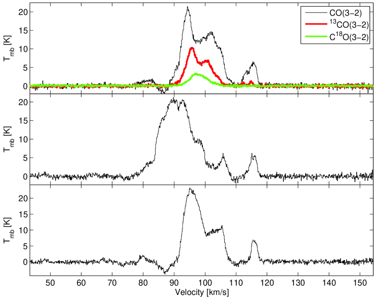
Figure 4: Spectra from ¹²CO $(J=3\rightarrow 2)$ are presented. Each spectrum corresponds to an average of nine pointings centered at offsets, from upper to bottom, ($\Delta\alpha$, $\Delta\delta$)=(0,0), (-90,-40), and (30,40), where the offsets are in arc-seconds. The velocity resolution for all the spectra is taken to be 0.1 km s^-1. The first panel also shows the spectra from ¹³CO $(J=3\rightarrow 2)$ in red and C¹⁸O $(J=3\rightarrow 2)$ in green. Clearly visible is the negative dip feature, likely due to emission in the off position, seen in both the upper and lower panels for the ¹²CO $(J=3\rightarrow 2)$ spectra. The component at 115 km s^-1 is also seen in both ¹²CO and ¹³CO but not in C¹⁸O.

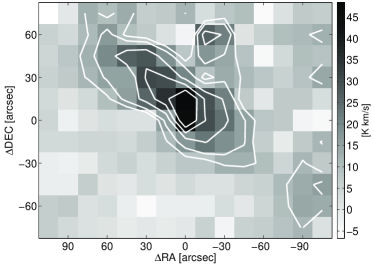
Figure 5: Velocity integrated emission map for HCO${}^{+}(J=4\rightarrow 3)$ over the whole velocity range (45 to 150 km s^-1) is shown. The pixel scale is in units of K km s^-1, while the contours are on levels of 3, 4, 6, 8, and 10 $\times$ $\sigma$, with $\sigma=3.7$ K km s^-1.

4.2 HCO${}^{+}(J=4\rightarrow 3)$ and H¹³CO${}^{+}(J=4\rightarrow 3)$ results

We observed HCO${}^{+}(J=4\rightarrow 3$) simultaneously with ¹²CO $(J=3\rightarrow 2)$, which also covered an area of $3.5^{\prime}\times 2.5^{\prime}$. The velocity integrated emission map is presented in Fig. 5. The morphology of the emission follows the same orientation south-west to north-east as the ¹²CO observations, but without the extension of ¹²CO. Clearly, the strongest emission is clustered at the center of the map, to the north-east, while some hint of emission over $3\sigma$ seems to appear at the south-west, roughly at ($\Delta\alpha,\Delta\delta$)=(-80^′′,-40^′′), where the strongest ¹²CO emission is located. The map morphology is also consistent with the HCO${}^{+}(J=3\rightarrow 2)$ map of Motte et al. (2003, see Fig. 2). Figure 6, central panel, shows the spectrum from the reference position for both HCO⁺ and H¹³CO⁺. The line profile is clearly non-Gaussian, showing evident self-absorption. It is likely that the HCO⁺ emission is optically thick. No hint of emission is seen at the off position, which is same off position used for ¹²CO. Superposed in thick lines is the H¹³CO${}^{+}(J=4\rightarrow 3)$ spectrum with a peak brightness temperature of 1.2 K at V=98.1 km s^-1. The H¹³CO⁺ emission is only significant (over the 3$\sigma$ level) at the reference position. The velocity associated with the peak can be considered to be at the $V_{\mathrm{lsr}}$ within the boundaries of the bin. The emission is also coincident with the strong absorption dip in HCO⁺, suggesting self-absorption. Additionally, because the line profile appears to be Gaussian in shape, it is likely that the H¹³CO⁺ emission is optically thin.

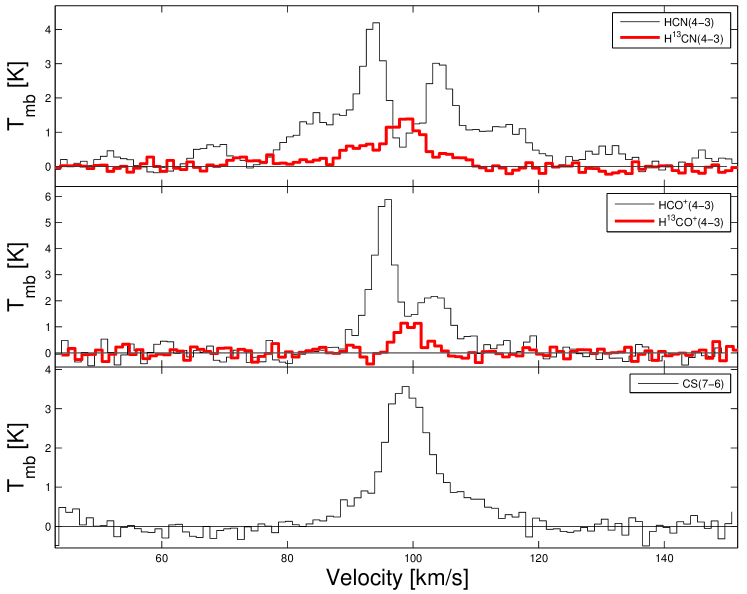
Figure 6: High density molecular gas spectra from the G30.79 FIR 10 clump. The upper panel presents the HCN$(J=4\rightarrow 3)$ spectrum. In thick red lines the H¹³CN$(J=4\rightarrow 3)$ spectrum is superposed. The central panel presents the HCO${}^{+}(J=4\rightarrow 3)$ spectrum. In thick red lines the H¹³CO${}^{+}(J=4\rightarrow 3)$ spectrum is superposed. The peak brightness temperature of H¹³CO⁺ is 1.2 K. The lower panel presents the CS$(J=7\rightarrow 6)$ spectrum. All spectra were taken at the reference position. Both HCO⁺ and the HCN spectra were binned every five channels, giving a velocity resolution of 0.54 km s^-1, while CS, H¹³CO⁺ and H¹³CN were binned every ten channels, giving a velocity resolution of 1.1 km s^-1.

4.3 CS$(J=7\rightarrow 6)$ results

The integrated velocity map for CS$(J=7\rightarrow 6)$ is presented in Fig. 7. As for H¹³CO⁺, the CS emission is fairly compact, arising only from the center of the map, which suggests that most of the activity is coincident with the peak of the dust emission. The spectra from the central 30${}^{\prime\prime}\times 30^{\prime\prime}$ are shown in Fig. 6 in the lower panel. The CS emission presents a peak brightness temperature of 3.6 K at V=98.1 km s^-1with some excess emission in its line-wings, which may be due to outflowing motions. Note that the CS emission is not self-absorbed as seen with HCO⁺ and HCN. It is possible that the molecule is not abundant enough to become self-absorbed. However, another possibility is that the CS gas is bound inside the dense core, which would explain why its emission is not widespread (as indicated by our map).

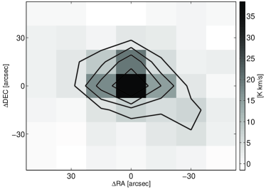
Figure 7: Velocity integrated emission map for CS$(J=7\rightarrow 6)$ over the whole velocity range (45 to 150 km s^-1). The pixel map has units of K km s^-1. The contour levels are 3, 6, 9, and 15 $\times\sigma$, with $\sigma=1.7$ K km s^-1.

4.4 HCN$(J=4\rightarrow 3)$ and H¹³CN$(J=4\rightarrow 3)$ results

The HCN$(J=4\rightarrow 3)$ was observed in position-switching mode over and area of $200^{\prime\prime}\times 150^{\prime\prime}$ to sample the same region as HCO⁺. We looked for emission only in the most significant areas within the region. The H¹³CN$(J=4\rightarrow 3)$ was only observed over the central $30^{\prime\prime}\times 30^{\prime\prime}$, where we expected to find most of the emission. Figure 8 presents the velocity integrated emission map for HCN. While the emission is mostly concentrated at the center, there is a hint for a gradient along the south-west to north east direction as with HCO⁺ and CO. The extent of the emission appears to be midway between the HCO⁺$(J=4\rightarrow 3)$ and the CS$(J=7\rightarrow 6)$ where the CS map presents the most compact morphology. Fig. 6 shows in its upper panel the HCN$(J=4\rightarrow 3)$ overlaid by the H¹³CN$(J=4\rightarrow 3)$ spectrum in red. The HCN emission is clearly opticaly thick with a self-absorption feature as indicated by the optically thin H¹³CN. The double peaked HCN spectrum has a stronger blue peak at 93.8 km s^-1; while the H¹³CN is peaked at 98.3 km s^-1, both taken from Gaussian fits. This type of spectrum is often seen toward infall candidates like the well-studied source B335 (Zhou et al., 1993).

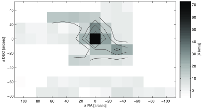
Figure 8: Velocity integrated emission map for HCN$(J=4\rightarrow 3)$. The integration is done over 60 to 140 km s^-1to include all the broad HCN emission. The pixel map has units of K km s^-1. The contour levels are 3, 6, 9, and 15 $\times\sigma$, with $\sigma=3.0$ K km s^-1. The color scale indicates the emission level with white used for positions not observed or with zero emission.

5 Analysis and discussion

5.1 The HCO⁺ abundance

In the current paradigm, it is suggested that carbon bearing molecules will freeze onto grain surfaces, forming ices, in cold and dense cores (see e.g. Bergin & Tafalla, 2007); while some other molecular abundances, like HCO⁺, might get enhanced by non-thermal motions such as outflows and/or infall (Rawlings et al., 2004). In order to investigate the abundance of HCO⁺ toward this region, we estimate the physical parameters associated with this molecule. The optical depth for HCO⁺ is estimated by the ratio between the optically thick and optically thin brightness temperatures by using (Choi et al., 1993)

$$\frac{T_{\mathrm{mb}4\rightarrow 3}}{T_{\mathrm{mb}(13)4\rightarrow 3}}=\frac{1-e^{-\tau_{43}}}{1-e^{-\tau_{43}/X}},$$ (1)

where $T_{\mathrm{mb}4\rightarrow 3}$ is the brightness temperature from the HCO⁺ line, $T_{\mathrm{mb}(13)4\rightarrow 3}$ is the H¹³CO⁺ line temperature, and $X$ is the ratio between $X$=[¹²C]/[¹³C] taken to be 50, a value representative for the molecular ring at the 4 kpc inner galaxy (Wilson & Rood, 1994). Because the HCO⁺ profile is self-absorbed, there is a significant uncertainty in deriving the line intensity. Two possible approaches can be followed: either we pick the strongest peak, or a Gaussian profile can be adjusted to the whole line by masking out the self absorption dip. Purcell et al. (2006) found no major differences from these two approaches in their results for a sample of 40 high-mass star forming regions. Thus, we used the strongest peak for the HCO⁺ line intensity in this calculation. From these numbers we obtained $\tau_{\mathrm{hco^{+}}}^{43}=11.3$ indicating an optically thick HCO⁺ line, which is to be expected due to the self-absorption seen in the line profile (see Fig. 6). Also, note that both the HCO⁺ and the H¹³CO⁺ line were obtained from the reference position and with a beam size of about $18^{\prime\prime}$, which encloses the dust core detected from the interferometric observations of this region (Cortes & Crutcher, 2006, see Figure 1).

To obtain the column density for the upper rotational level, we use (Goldsmith & Langer, 1999)

$$N_{4}=\frac{8\pi k\nu^{2}}{hc^{3}A_{43}}\left(\frac{\Delta\Omega_{a}}{\Delta\Omega_{s}}\right)\left(\frac{\tau_{43}}{1-e^{-\tau_{43}}}\right)\int T_{\mathrm{mb}}dv,$$ (2)

where $\nu$ is the line frequency, $A_{43}$ is the Einstein spontaneous emission coefficient ($3.6269\times 10^{-3}$ s^-1 for HCO${}^{+}(J=4\rightarrow 3)$), $\Delta\Omega_{a}$ is the antenna solid angle and $\Delta\Omega_{s}$ is the source solid angle for the core which gives a beam filling factor of $0.73$ for HCO⁺. The total column density is then given by

$$N=\frac{N_{u}Z}{ge^{-E_{u}/T}},$$ (3)

where $Z$ is the partition function, $g=2J+1$ is the statistical weight of the upper level, $E_{u}=42.8$ K is the energy for the upper level (Schöier et al., 2005), and $T=30$ K is the dust temperature used by Cortes & Crutcher (2006) to calculate the total hydrogen column density $N$(H₂). This is justified under the LTE assumption. For linear molecules, the partition function is well approximated by $Z=kT/hB_{0}$, where $B_{0}=45$ GHz is the rotational constant for HCO⁺ taken from Defrees et al. (1982). In this way, we estimated a HCO⁺ column density $N$(HCO⁺) = 1.5 $\times 10^{14}$ cm^-2. From a sample of 40 high-mass star forming regions selected from methanol maser detections, Purcell et al. (2006) estimated the HCO⁺ column densities ranging from 2.5$\times 10^{14}$ cm^-2 to 71 $\times 10^{14}$ cm^-2. Our column density estimation is consistent with the smallest values obtained in their work. Now, by using the column density of hydrogen derived from dust emission or $N$(H₂) = 6.5 $\times 10^{23}$ cm^-2, we calculate a total abundance for HCO⁺ or $X$(HCO⁺) = 2.4 $\times 10^{-10}$. As previously mentioned, it is expected that carbon bearing molecules will get depleted toward cold and dense regions. We can quantify this by calculating the depletion factor $f_{D}$ defined as the ratio between the average fractional abundance and the observed one. Lucas & Liszt (1996) and Liszt & Lucas (2000) determined a $X_{\mathrm{ISM}}=2\times 10^{-9}$ from a sampling of HCO${}^{+}(J=1\rightarrow 0)$ toward the diffuse ISM in absorption against background QSOs. By using this value for $X_{\mathrm{ISM}}$, we find $f_{D}=8.4$, which suggests that a moderate depletion of HCO⁺ toward this clump when compared to other high-mass star forming regions such as G305 with $f_{D}=1.5$ (Walsh & Burton, 2006; Bergin et al., 1997). However, we maybe underestimating the HCO⁺ column density due to the uncertainty introduced by the brightness temperature used from the observed self absorbed profile, which would lead a lower depletion value for HCO⁺. These results, along with the lack of infrared sources detected at this clump, and with no compelling evidence for outflow emission, even though maser emission has been observed (see next section), suggest an early (pre-hot core) evolutionary stage for G30.79 FIR 10. In an advanced stage, it is expected that the radiation coming from the central condensation will evaporate the ice mantles increasing the abundance of molecules like HCO⁺, creating what is known as a hot core. Note though, that the detection of maser emission toward this clump suggests that the star formation process has already started.

5.2 An outflow in G30.79 FIR 10?

One of the signatures of high-mass star formation are the powerful molecular outflows observed toward these regions (Shepherd et al., 2007; Bourke et al., 1997). Because FIR 10 is a massive core, it is likely that outflowing motions are present or will develop over time. However, to untangle the outflow motions from our molecular emission observations is certainly not trivial. The choice of sub-millimeter emission lines as a tool to study this region allow us to separate the most dense components from the rest of the molecular core. Particularly, ¹²CO $(J=3\rightarrow 2)$ has been successfully used to trace outflowing motion from star forming regions (Choi et al., 1993). However, our ¹²CO $(J=3\rightarrow 2)$ results are inconclusive because of emission at the off position, which affected the line wings in our spectra. Also, the high velocity component seen at V=115 km s^-1, which is $\sim$20 km s^-1 over the $V_{\mathrm{lsr}}$ and is only seen in ¹²CO and ¹³CO but not observed either in HCO⁺, HCN, or CS. It is likely that this component is not dense enough to excite either of these lines; indeed, this high velocity component might be optically thin. Although it could be interpreted as high velocity outflow emission, its widespread spatial distribution makes this interpretation un-likely. Another possibility is that this component corresponds to a foreground object, or cloud, which is not associated with this clump. Additionally, it is difficult to accelerate the gas to such high velocities without dissociation.

Outflows are discovered through their signature in the line-wings of molecular emission lines. Fig. 9 shows the HCO⁺ and CS spectra with their corresponding Gaussian fittings and the residual emission in their line-wings. Between 100 and 110 km s^-1we found some significant emission over the $3\sigma$ level, with $\sigma=0.08$ K, in both CS and HCO⁺ spectrum. However, the blue-shifted part of the emission, for velocities lower than 95 km s^-1, does not show significant traces of residual emission. Even though the red-shifted excess emission may be due to non-thermal motions, the bipolar nature of an outflow must be clearly stated, which we cannot do with these data. Therefore, we cannot yet come to a conclusion about the presence of a bipolar outflow towards this source. Our lack of spatial resolution due to the distance to G30.79 FIR 10 might be the reason behind this. However, outflows are ubiquitous in the high-mass star forming regions, so it is likely that they are present or will develop over time. Additional observations of shocked excited chemistry, such as SiO, SO, or SO₂ may help confirming an outflow in this clump.

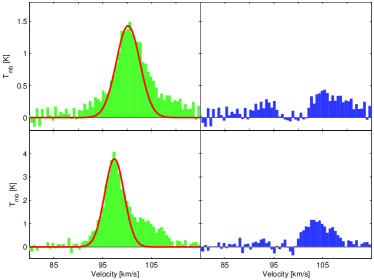
Figure 9: Residual emission after Gaussian substraction is shown in both panels. The lower panel shows the HCO${}^{+}(J=4\rightarrow 3)$ profile with an adjusted Gaussian to the left. To the right, in the same panel, the residual emission from the Gaussian subtraction is presented. The upper panel shows CS$(J=7\rightarrow 6)$ profile with the adjusted Gaussian profile and its residual emission to the right. The $\sigma$ value is calculated to be 0.08 K. Both spectra were taken as averages over an area of $30^{\prime\prime}\times 30^{\prime\prime}$.

5.3 Infall motions

It is not clear whether high-mass stars forms through accretion or through a different process such as coalescence of less massive fragments. This situation is difficult to distinguish due to the physical complexities involved in the evolution of high density gas and dust. The study of the kinematics and dynamics at the earliest phases, along with the detection of accretion disks, could clarify this uncertainty. In this scope, the determination of infalling motions is a first step toward the identification of collapsing pre-stellar objects. The characterization of these motions is a challenging topic, the current avenue towards investigating infalling is the study of asymmetries in molecular line profiles. Leung & Brown (1977) suggested that an asymmetry in the line profile toward the blue may indicate the presence of infalling motions. Thus, the low excitation, red-shifted infalling layers of gas in the front part of the cloud absorbs some of the emission from the rest of the gas. This red-shifted self-absorption is what makes the spectrum present a brighter blue peak. To quantify this asymmetry, the calculation of the normalized line velocity difference has been used by many authors (Fuller et al., 2005; Szymczak et al., 2007; Wu et al., 2007).

$$\Delta V_{\mathrm{be}}=\frac{V^{\mathrm{max}}_{\mathrm{thick}}-V^{\mathrm{max}}_{\mathrm{thin}}}{\Delta V_{\mathrm{thin}}},$$ (4)

where $V^{\mathrm{max}}_{\mathrm{thick}}$ is the velocity from the peak emission of the optically thick line, $V^{\mathrm{max}}_{\mathrm{thin}}$ is the velocity from the peak emission of the optically thin line, and $\Delta V_{\mathrm{thin}}$ is the FWHM line width from the optically thin molecular tracer. A negative $\Delta V_{\mathrm{be}}$ will correspond to blue-shifted gas velocities, which are indicative of infalling motions. We calculated $\Delta V_{\mathrm{be}}$ for the high density tracers HCN, CS, and HCO⁺ using H¹³CO⁺ and H¹³CN as the optically thin tracers. These molecules have high dipole moments and therefore require higher critical densities to get excited. In particular we used H¹³CO⁺ as the thin component for HCO⁺ and H¹³CN for CS and HCN to keep ion-molecules and neutral molecules separate. Table 3 gives the values of $\Delta V_{\mathrm{be}}$ for all three lines. The difficulty in separating infalling evidence from the line asymmetry arises because other dynamic phenomena such as rotation and outflows will also produce red and blue asymmetries in the molecular profiles. However, infalling is the only motion which will produce only blue asymmetries. The expected infall signature will manifest in spectral lines with a double peaked profile where the blue peak is stronger than the red peak and the dip is due to self absorption. A blue asymmetry is seen in all spectra, with the highest value in HCO⁺, but the characteristic infalling double peak profile is only seen in both HCN and HCO⁺. Both appear to be self absorbed and have a stronger blue component (see Fig. 6). The case of HCO⁺ is interesting, the red component is almost non-existent having the largest blue asymmetry in all three molecules. The CS spectrum is single peaked to the blue, but does not show the self-absorbed features. It has the lowest intensity, which could be cause by carbon and sulfur depletion in this object. In this way, it may not have enough abundance to self-absorb. Evans (2003) suggested a procedure to evaluate whether infall is likely or not in a star forming core. We followed the procedure checklist and found that our HCN observations, taken at the reference position, meet the conditions required for infall. Moreover, the same properties are observed in the HCN spectra from the surrounding pointings (see Fig. 10). Almost all of them present double peaked profiles with a stronger blue peak, clearly suggesting infalling. Together with the previous checklist we can conclude that our HCN spectra meet the requirements to suggest infall movements toward this source. Thus, we quantified the infall parameters through modeling. To do this, we applied the simple infalling model devised by Myers et al. (1996) and later improved by Di Francesco et al. (2001). In this model, the clump is approximated by two infalling gas layers, a front and a rear layer, with a central source modeling the pre-stellar core. Thus, the observed brightness temperature is quantified by the following equation, where the subscripts $``$f”, $``$r”, $``$C”, and $``$cmb” stand for the front layer, the rear layer, the central source, and the cosmic background.

Table 2: Parameters from the model fit

$J(T_{\mathrm{f}})$	$J(T_{\mathrm{r}})$	$v_{\mathrm{f}}$	$v_{\mathrm{r}}$	$\tau_{0}$	$\sigma$
$[\mathrm{K}]$	[K]	[km s-1]	[km s-1]	-	[km s-1]
24.6	17.5	0.7	-0.3	2.0	3.4

The parameters from the best fit obtained by adjusting the Di Francesco et al. (2001) infalling model to our HCN($J=4\rightarrow 3$) spectrum.

$$\Delta T_{\mathrm{B}}=(J_{\mathrm{f}}-J_{\mathrm{C}})[1-e^{-\tau_{\mathrm{f}}}]+(1-\Phi)(J_{\mathrm{r}}-J_{\mathrm{cmb}})[1-e^{-(\tau_{\mathrm{r}}+\tau_{\mathrm{f}})}].$$ (5)

The main terms in this equation are the Planck excitation temperature given by $J_{\mathrm{i}}=T_{0}/[\exp{(T_{0}/T_{\mathrm{i}})}-1]$ with $T_{0}=h\nu/k$, and $T_{\mathrm{i}}$ corresponding to either $T_{\mathrm{f}}$, $T_{\mathrm{r}}$, $T_{\mathrm{c}}$, and $T_{\mathrm{cmb}}$. Also, $J_{\mathrm{C}}=\Phi J_{\mathrm{c}}+(1-\Phi)J_{\mathrm{r}}$ where $\Phi$ is the beam filling factor of the continuum source, which due to our large beam size is assumed to be 0. The $\tau_{\mathrm{i}}$ expressions correspond to the optical depths, which we assumed to be Gaussian (following Myers et al., 1996). Thus, the front and rear optical depths are given by

$$\tau_{\mathrm{f}}=\tau_{0}\exp{\left[\frac{-(v-v_{\mathrm{f}}-v_{\mathrm{lsr}})^{2}}{2\sigma^{2}}\right]}$$ (6)

$$\tau_{\mathrm{r}}=\tau_{0}\exp{\left[\frac{-(v+v_{\mathrm{r}}-v_{\mathrm{lsr}})^{2}}{2\sigma^{2}}\right]},$$ (7)

where $\tau_{0}$ is the peak optical depth for both the front and the rear layers, $v_{\mathrm{f}}$ and $v_{\mathrm{r}}$ are the infalling velocity for both slabs and $\sigma$ is the velocity dispersion. The model was fitted in a two step process, first by doing a multi Gaussian fit component, which provided the input parameters to later adjust Eqn. 5 to our data by minimizing the $\chi^{2}$ function through the Levenburg-Marquardt algorithm (Press, 2002). The best fit to the HCN spectrum is shown in Fig. 11, and the fit parameters are presented in Table 2. Note that this is the simplest possible model that we can use to characterize infalling gas. Moreover, the structure of the HCN line is complex and, even though the features seen in the line wings may come from outflowing motions, we did not consider them in this simple model.

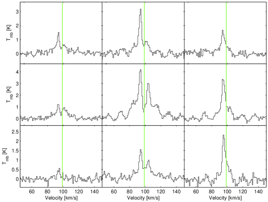
Figure 10: The central $48^{\prime\prime}\times 48^{\prime\prime}$ region compose of 9 pointings separated by $15^{\prime\prime}$ with a beam size of $18^{\prime\prime}$ each is shown. The green line represents the systemic velocity at 98.8 km s^-1; while the scale is given in K (main beam temperature)

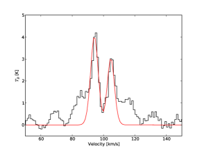
Figure 11: Central HCN spectrum from G30.79 FIR 10. Overlaid in thick lines is the best fit for the infalling model.

The infalling velocity for both slabs is estimated by the infalling model to be $v_{\mathrm{f}}=0.7$ km s^-1and $v_{\mathrm{r}}=-0.3$ km s^-1. A simple estimation can also be done by using the analytical model derived by Myers et al. (1996) for a contracting cloud. By using Eqn. 9, from their model, we estimated an infalling velocity of 0.5 km s^-1. This result is in good agreement with the the values obtained by adjusting the model to our data. The next step is to estimate the mass infall rate, which we do by following (Klaassen & Wilson, 2007)

$$\dot{M}=\frac{\mathrm{d}M}{\mathrm{d}t}\approx\frac{M}{t}=\frac{\rho Vv_{\mathrm{in}}}{R}=\frac{4}{3}\pi n_{\mathrm{H}_{2}}\mu m_{\mathrm{H}}R^{2}v_{\mathrm{in}},$$ (8)

where $\mu=2.35$ is the mean molecular weight, $R=0.3$ pc is the geometric radius taken from the interferometric observations, and $n_{\mathrm{H}_{2}}$ is the gas density. The infall rate obtained for this source is about $5\times 10^{-3}$ M_⊙/yr. Both infall velocity and infall mass rate are consistent with the values seen at other high-mass star forming regions, like G10.47, which has an estimated infall velocity of 1.8 km s^-1and an infall rate of $10^{-2}$ M_⊙/yr (Klaassen & Wilson, 2007). Barnes et al. (2008) estimated infall rates of $3\times 10^{-2}$ M_⊙/yr with an infalling velocity of 0.3 km s^-1for the G286.21+0.17 molecular clump. Both regions present similar gas densities as G30.79 FIR 10 ($1.9\times 10^{5}$ cm^-3 for G286.21+0.17 and $7.2\times 10^{5}$ cm^-3 for G10.47) and similar mass estimations ($4.1\times 10^{4}$ M_⊙for G286.21+0.17 and $7.3\times 10^{3}$ M_⊙ for G10.47 Shirley et al., 2003, as estimated by). These results are consistent with our findings where these regions appear to be in a similarly evolutionary stage.

Table 3: Normalized velocity difference.

Line	$\Delta V_{\mathrm{be}}$
HCN$(J=4\rightarrow 3)$	-1.1
HCO${}^{+}(J=4\rightarrow 3)$	-1.2
CS$(J=7\rightarrow 6)$	-0.1

The asymmetry of line profiles is presented by the calculation of $\Delta V_{\mathrm{be}}$, as shown in Eqn. 4, where the optically thin species correspond to H¹³CO⁺ for HCO⁺ and H¹³CN for HCN and CS. The values used to compute the blue excess are taken from Gaussian fits to the corresponding spectra.

5.4 Dynamical state of G30.79

5.4.1 The magnetic field

The dynamical state of high-mass star forming cores is difficult to establish. The accumulation of a large amount of molecular gas is still poorly understood, as is what triggers the gravitational collapse. Moreover, it is known that magnetic fields are present in these regions with strengths substantially larger than in low-mass star forming regions (Lai, 2001; Cortes & Crutcher, 2006). Thus, the magnetic field can have a profound effect on the dynamical evolution of the gas as postulated by ambipolar diffusion theories (Ciolek & Mouschovias, 1993). Our object of study is not an exception to the above. Magnetic fields have been observed through polarized emission from dust towards this core (Vallée & Bastien, 2000; Cortes & Crutcher, 2006). However, it is not yet clear how important the field is with respect to turbulence in the high-mass star forming process, but its presence alone is a reason to consider its effects.

From the interferometric observations of polarized dust emission, Cortes & Crutcher (2006) found a smooth polarimetric pattern centered at the G30.79 FIR 10 clump. Assuming magnetic alignment of dust grains, they proposed an hourglass morphology for the field. Additionally, they estimated the magnetic field strength on the plane of the sky using the Chandrasekhar-Fermi method (Chandrasekhar & Fermi, 1953), finding a value of $B_{\mathrm{pos}}=1.7$ mG. In this way, the mass-to-magnetic flux ratio was calculated to be $\lambda=0.9$ or critical. In this work, we refined the previously described estimation by considering our molecular line observations. Before stating this improvement, we will briefly introduce the Chandrasekhar-Fermi method by the following equation.

$$B_{\mathrm{pos}}=9.3\frac{\sqrt{n(\mathrm{H_{2}})}\Delta V}{\delta\phi},$$ (9)

where $B_{\mathrm{pos}}$ is the magnetic field strength in $\mu$G, $n$(H₂) is the volumetric gas number density in cm^-3, $\Delta V$ is the FWHM velocity width in km s^-1, and $\delta\phi$ is the polarization position angle dispersion in degrees. Cortes & Crutcher (2006) used $n$(H₂) = 4.5$\times 10^{5}$ cm^-3 calculated from their dust emission, while $\delta\phi=21^{\circ}.9$ was obtained from the polarization data. The line-width, $\Delta V$, was taken from the H¹³CO${}^{+}(J=3\rightarrow 2)$ observations by Motte et al. (2003) for the G30.79 clump (called MM1 and listed at Table 2 in their work). It is here where we improve the estimation by using $\Delta V$ derived from our H¹³CO${}^{+}(J=4\rightarrow 3)$ observations. The $(J=4\rightarrow 3)$ transition traces higher density molecular gas, while being better coupled to the field than H¹³CN or other neutral species. Also, the H¹³CO${}^{+}(J=4\rightarrow 3)$ emission is optically thin, which might not be the case for the $(J=3\rightarrow 2)$ transition. Additionally, this higher transition comes from a smaller beam size, which engulfs only the FIR 10 clump (of about 20^′′ in size), while the $(J=3\rightarrow 2)$ transition comes a higher beam size ($\sim 30^{\prime\prime}$), which might be including velocity components not associated to the field perturbations. Thus, by using $\Delta V=3.0$ km s^-1 we obtain a value for $B_{\mathrm{pos}}=$855 $\mu$G, which gives a statistically corrected mass-to-magnetic flux of $\lambda=1.9$, or super-critical, consistent with the infalling scenario suggested in this work. Thus, the magnetic field is not strong enough to support the core.

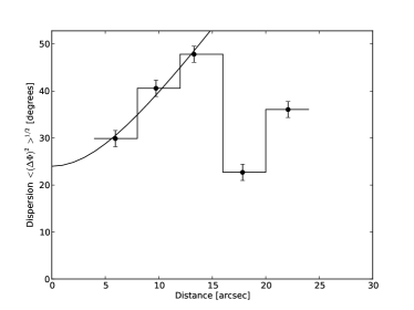
Figure 12: The polarization position angle dispersion function is shown here in closed circles along with its respective error bars. The dispersion function points are join with thick lines, while superposed is the fit for Equation 10 to the first 3 points.

While the polarization pattern observed by Cortes & Crutcher (2006) is smooth, it is unclear how distorted by turbulence the field might be. This source is 5.5 kpc away which gives 0.03 pc/1^′′ or 0.1 pc/beamsize. This length scale is larger than the predicted turbulence length scale of 1 mpc (Yan et al., 2004; Li & Houde, 2008). Therefore, the dispersion in the field lines, or the turbulent component of the field, cannot be directly seen from the polarization pattern. Hildebrand et al. (2009) developed an approximation to calculate the plane of the sky dispersion function for the magnetic field in turbulent molecular clouds. By using polarized emission from dust, they calculated a dispersion function for the polarization position angle as a quadratic function of the length scale. Two main assumptions are made in this calculation. The length scale is larger than the turbulence, or correlation length scale, and smaller than the length scale associated with large scale variations of the field. Our BIMA polarization data satisfy both assumptions, the interferometric observations have a length scale on the order of 0.1 pc while the field varies over 1 pc distances (as seen from the polarization pattern). This approximation is stated in Eqn. 2 in Hildebrand et al. (2009). From this approximation, the ratio between the turbulent component of the field on the plane of the sky and the main magnetic field strength can be estimated as

$$\frac{\left<B_{t}^{2}\right>}{B_{0}}=\frac{b}{\sqrt{2-b^{2}}},$$ (10)

where $b$ is the turbulent contribution to the dispersion function, $\left<B_{t}^{2}\right>$ is the turbulent component of the field, and $B_{0}$ is the main magnetic field. We applied this method to our BIMA data by calculating the dispersion function for polarization position angle as shown in Fig. 12. The value of $b=0.42$ is given by the intersect of the best fit to the data points, and gives a turbulent-to-main magnetic field ratio of $\left<B_{t}^{2}\right>/B_{0}=0.3$. This result suggest that 30% of the total magnetic field strength is in the turbulence.

5.4.2 The gravitational equilibrium in G30.79 FIR 10

This source is one of the few where information about the magnetic field and turbulence is present. Thus, we should be able to characterize with confidence the state of gravitational equilibrium in this source. In order to quantify this, we will follow the analysis as stated by McKee & Zweibel (1992) and Bertoldi & McKee (1992):

$$2(\mathcal{T}-\mathcal{T}_{0})+\mathcal{M}+W=0$$ (11)

where $\mathcal{T}$ is the total kinetic energy including thermal and non-thermal motions, $\mathcal{T}_{0}$ correspond to the surface term for the kinetic energy, or external pressure, $\mathcal{M}$ is the magnetic energy, and $W$ is the gravitational energy term. We will follow Motte et al. (2003) and assume the giant HII region present in the W43 complex does not reach the clump. In this way, we can drop $\mathcal{T}_{0}$ out the equation. Only the kinetic and magnetic terms remains to balance gravity and as was said before, we have information about both of them.

Motte et al. (2003) estimated the virial mass without knowing the magnetic field, stating that G30.79 FIR 10 is likely to be bound. To estimate the virial mass they used $M_{\mathrm{vir}}=5R\sigma^{2}/G$ from Bertoldi & McKee (1992), which we refined by deriving our own values for $R=0.3$ pc (obtained from the interferometric map of dust emission from Cortes & Crutcher 2006 as half the size of the continuum core or $10^{\prime\prime}$), and $\sigma=1274$ m s^-1 from our H¹³CO⁺ observations ($\sigma$ is not the FWHM value), obtaining $M_{\mathrm{vir}}=563$ M_☉. Comparing this with the mass of the clump taken to be M_submm = 3300 M_☉ (Cortes & Crutcher, 2006) we obtained the ratio of the virial mass to the dust mass to be M_submm/M${}_{\mathrm{vir}}=5.9$. Values of M_submm/M${}_{\mathrm{vir}}>0.5$ are considered to remain gravitationally bound according to Pound & Blitz (1993). At the same time, we recall our previous calculation of the mass-to-magnetic flux ratio, which was found to be super-critical. This means that there is not enough energy in the turbulence and/or in the magnetic field to balance gravity. Therefore and even though the uncertainties involved in the total mass estimations for this object, the results suggest that G30.79 FIR 10 is bound and must be undergoing gravitational collapse. The whole picture appears to be self-consistent, we have detected infalling motions into the clump where neither turbulence or the magnetic field have enough energy to counterbalance gravity.

6 Summary and conclusions

We mapped the G30.79 FIR 10 molecular clump embedded in the W43 mini-starburst by mapping the molecular emission from ¹²CO$(J=3\rightarrow 2)$, ¹³CO$(J=3\rightarrow 2)$, C¹⁸O$(J=3\rightarrow 2)$, CS$(J=7\rightarrow 6)$, HCO${}^{+}(J=4\rightarrow 3)$, H¹³CO${}^{+}(J=4\rightarrow 3)$, HCN$(J=4\rightarrow 3)$, and H¹³CN$(J=4\rightarrow 3)$. Emission from ¹²CO is extended presenting a gradient from south-west to north-east, consistent with the dust morphology of the core. Even though we mapped ¹³CO from a smaller region surrounding the center, its emission appears to follow ¹²CO, which is also optically thick. The C¹⁸O emission was also mapped at the central $30^{\prime\prime}\times 30^{\prime\prime}$. Its line profile is almost Gaussian without any of the complex features seen in the previous CO isotopomers and is likely optically thin. We found a high velocity component at 115 km s^-1, which was also present all over our sampled region. We interpreted this emission as a foreground cloudlet not associated with our clump. The emission from HCO⁺ is optically thick, with an optical depth $\tau=11.3$, but more compact than ¹²CO. This is expected due to the higher densities required to excite this molecule. Additionally, both CS and H¹³CO⁺ are even more compact, with the emission coming mostly from the central $30^{\prime\prime}\times 30^{\prime\prime}$ and consistent with the position of the dust maxima obtained by others. By using our observations, we estimated the HCO⁺ abundance $X$(HCO⁺)=2.4 $\times$ $10^{-10}$, a depletion factor $f_{D}=8.4$, which is consistent with estimations done toward other high-mass star forming regions (Purcell et al., 2006).

Outflows were looked for in the line-wings of the observed molecular lines toward the center of G30.79 FIR 10. All HCO⁺, HCN, and CS profiles present excess emission in their line wings. However, the bipolar nature of this emission is inconclusive at the $3\sigma$ level. Infalling motions were also looked for by studying the profile asymmetry of our molecular observations. The blue asymmetry was estimated by calculating the normalized velocity difference (see Table 3). The clearest evidence for infall is given by the HCN spectra. Toward the center and surroundings pointings, the emission is double peaked with the blue peak stronger than the red peak (see Fig. 6 and 10). By using the Myers et al. (1996) improved model by Di Francesco et al. (2001), we estimated an infall velocity of 0.5 km s^-1with an infall rate of $5\times 10^{-3}$ M_⊙/yr.

We refined a previous estimate for the magnetic field strength on the plane of sky in this region. Interferometric observations of polarized emission from dust from Cortes & Crutcher (2006) estimated a magnetic field of $B_{\mathrm{pos}}$=1.7 mG, by using the Chandrashekar-Fermi technique. The estimation needs a reliable tracer for the gas turbulent motions from the region traced by the dust emission. By using the line-width from our ion optically thin molecule H¹³CO${}^{+}(J=4\rightarrow 3)$, $\Delta V=3$ km s^-1, we were able to obtained an improved estimation of $B_{\mathrm{pos}}=$855 $\mu$G for the magnetic field, which also refined the mass-to-magnetic flux ratio to $\lambda$=1.9 or super-critical. Along with $\lambda$, we calculated the contribution from turbulence to the virial mass, getting a value of M_submm/M${}_{\mathrm{vir}}=5.9$. These two results suggest that neither the magnetic field nor the turbulence have enough energy to counterbalance gravity. Therefore, the G30.79 FIR 10 clump must be bound and undergoing gravitational collapse. This also reinforce the core as an infall candidate.