0 [

] Cinderella User’s Manual

P. Reegen¹

¹ Institut für Astronomie, Türkenschanzstraße 17, 1180 Vienna, Austria
reegen@astro.univie.ac.at

Abstract

Cinderella is a software solution for the quantitative comparison of time series in the frequency domain. It assigns probabilities to coincident peaks in the DFT amplidude spectra of the datasets under consideration. Two different modes are available. In conditional mode, Cinderella examines target and comparison datasets on the assumption that the latter contain artifacts only, returning the conditional probability of a target signal, although there is a coincident signal in the comparison data within the frequency resolution. In composed mode, the probability of coincident signal components in both target and comparison data is evaluated. Cinderella permits to examine multiple target and comparison datasets at once.

1 What is Cinderella?

Cinderella is an abbreviation of “Comparison of INDEpendent RELative Least-squares Amplitudes”. It provides a quantitative comparison between the DFT amplitude spectra of time-resolved astronomical measurements.

The SigSpec technique (Reegen 2005, 2007) allows to determine probabilities for coincident peaks in the DFT amplitude spectra of different datasets quantitatively and in a statistically unbiased way. The theoretical background of this procedure is introduced by Reegen et al. (2008).

Cinderella uses the standard output of the program SigSpec, which represents the results of a cascade of consecutive prewhitenings employing least-squares fits to obtain amplitudes and phases of signal components. Following the SigSpec terminology, Cinderella returns a spectral significances (hereafter abbreviated by ‘sig’) rather than a probability. This manual uses cross-references to SigSpec frequently. In these cases, the reader is referred to the SigSpec manual (Reegen 2009).

2 Projects

Cinderella is called by the command line

Cinderella <project>

where <project> is the name (or path, if desired) of the Cinderella project. The project structure is strictly consistent with SigSpec.

Before running the program, the user has to provide

1. at least two time series input files consistent with the SigSpec MultiFile mode (see SigSpec manual, p. LABEL:SIGSPEC_MultiFile_Mode, and “Time series input files”, p. 1), and

2. a directory <project> containing the SigSpec result files corresponding to the time series input files (see “SigSpec result files”, p. 2).

Furthermore, the user may pass a set of specifications to Cinderella by means of a file <project>.cnd (see “The .cnd file”, p. 3). This file is expected in the same folder as the time series input files and the project directory. For specifications not given by the user, defaults are used.

Cinderella is designed to answer two different questions, depending on the problem it is applied to. By default, the program runs through both modes simultaneously and provides both conditional (p. 6) and composed sigs (p. 7).

3 Input

1 Time series input files

Cinderella expects at least two time series input files named according to #index#.<project>.dat. In this context, #index# is a placeholder for a six-digit index of the file. Note that only files with consecutive indices are appropriately recognised by Cinderella. The conventions are compatible with the SigSpec MultiFile mode (see SigSpec manual, p. LABEL:SIGSPEC_MultiFile_Mode), whence the most convenient preparation of data for Cinderella is the SigSpec MultiFile computation.

The only restrictions to the format of the time series input files are that the number of items per row has to be constant for all rows in the file and that the columns have to be seperated by at least one whitespace character or tab. Dataset entries need not to be numeric, except for the columns specified as time, observable, and weights. The conventions for specifying these three column types are consistent with SigSpec. See SigSpec manual, pp. LABEL:SIGSPEC_Time_series_columns_representing_time_and_observable, LABEL:SIGSPEC_Time_series_columns_containing_statistical_weights for details.

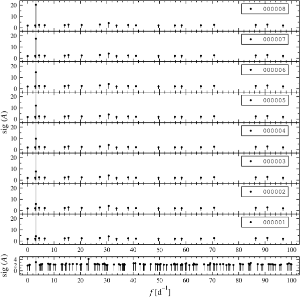
Figure 1: SigSpec result files used as input for the sample project CinderellaNative. The bottom panel refers to the file CinderellaNative/000000.result.dat, which is used as the comparison dataset. Above, the files CinderellaNative/000001.result.dat to CinderellaNative/000008.result.dat are displayed from bottom to top. The underlying time series represent Gaussian noise plus a single sinusoidal signal at a frequency of $3.125\,\mathrm{d}^{-1}$ (grey line) with different amplitudes.

2 SigSpec result files

The SigSpec result files #index#.result.dat are located in the project directory and contain a list of all sig maxima associated to each of the input time series #index#.<project>.dat. A SigSpec result file consists of seven columns. A full description is provided by the SigSpec manual, p. LABEL:SIGSPEC_Result_files. Cinderella uses only five columns:

• the frequency [inverse time units] (column 1),

• the sig (column 2),

• the amplitude [units of observable] (column 3),

• rms scatter of the time series before prewhitening (column 5), and

• point-to-point scatter of the time series before prewhitening (column 6).

The last line of a result file contains only two non-zero values in columns 5 and 6. These represent the rms and point-to-point scatter of the time series after the last prewhitening step, correspondingly, and are also used by Cinderella.

Example. The sample project CinderellaNative provides a run without any additional options by typing Cinderella CinderellaNative. The files 000000.CinderellaNative.dat, …, 000008.CinderellaNative.dat are the same as 000038.diffsig.dat to 000046.diffsig.dat in the SigSpec example diffsig (Reegen 2009, p. LABEL:SIGSPEC_EXdiffsig), correspondingly.

The SigSpec result files 000000.result.dat to 000008.result.dat are provided in the project directory CinderellaNative. They contain all signal components found with sig $>$ 2 and are displayed in Fig. 1.

The screen output at runtime starts with a standard header.

 CCCCC  ii            dd                      ll  ll
CC   CC               dd                      ll  ll
CC      ii n nnn   ddddd  eeee  r rrr   eeee  ll  ll   aaaa
CC      ii nn  nn dd  dd ee  ee rr  rr ee  ee ll  ll  aa  aa
CC      ii nn  nn dd  dd ee  ee rr     ee  ee ll  ll      aa
CC      ii nn  nn dd  dd eeeeee rr     eeeeee ll  ll   aaaaa
CC      ii nn  nn dd  dd ee     rr     ee     ll  ll  aa  aa
CC   CC ii nn  nn dd  dd ee  ee rr     ee  ee ll  ll  aa  aa
 CCCCC  ii nn  nn  ddd d  eeee  rr      eeee   ll  ll  aaa a


Comparison of INDEpendent RELative Least-squares Amplitudes
Version 1.0
************************************************************
by Piet Reegen
Institute of Astronomy
University of Vienna
Tuerkenschanzstrasse 17
1180 Vienna, Austria
Release date: April 29, 2008

The program starts with processing the command line, checking if a present directory CinderellaNative is present, and searching for a configuration file CinderellaNative.cnd (see “The .cnd file”, p. 3). Since there is no such file present, Cinderella produces a warning message.

*** start **************************************************

Checking availability of project directory CinderellaNative...
project directory CinderellaNative ok.

Warning: CndFile_LoadCnd 001
         Failed to open .cnd file.

Now Cinderella counts the time series input files and checks for corresponding SigSpec result files.

*** MultiFile count ****************************************

Number of files                           9

The next step is to count the rows in each SigSpec result file.

*** count rows in SigSpec result files *********************

CinderellaNative/000000.result.dat:    106 rows
CinderellaNative/000001.result.dat:     21 rows
CinderellaNative/000002.result.dat:     21 rows
CinderellaNative/000003.result.dat:     21 rows
CinderellaNative/000004.result.dat:     21 rows
CinderellaNative/000005.result.dat:     21 rows
CinderellaNative/000006.result.dat:     21 rows
CinderellaNative/000007.result.dat:     21 rows
CinderellaNative/000008.result.dat:     21 rows

Before reading the input files, Cinderella performs the assignment of target, comp and skip tags to the datasets (see “Dataset Types”, p. 5). Since there is no file CinderellaNative.cnd available, the defaults are used: the first file, 000000.CinderellaNative.dat is considered a comparison dataset, the eight remaining files are interpreted as targets.

*** dataset type assignment ********************************


Warning: CndFile_Cind 001
         Failed to open .cnd file.
         Assigning default types.

000000.CinderellaNative.dat: comparison (default)
000001.CinderellaNative.dat: target (default)
000002.CinderellaNative.dat: target (default)
000003.CinderellaNative.dat: target (default)
000004.CinderellaNative.dat: target (default)
000005.CinderellaNative.dat: target (default)
000006.CinderellaNative.dat: target (default)
000007.CinderellaNative.dat: target (default)
000008.CinderellaNative.dat: target (default)

number of target datasets                 8
number of comparison datasets             1
number of datasets to skip                0

The time series and SigSpec result files are read, and Cinderella displays the frequency resolution and the mean observable for each time series.

*** read input files ***************************************

000000.CinderellaNative.dat: Rayleigh resolution 0.1089880382935977
000000.CinderellaNative.dat: mean observable     0.0074422789800987
CinderellaNative/000000.result.dat
000001.CinderellaNative.dat: Rayleigh resolution 0.0914470160931467
000001.CinderellaNative.dat: mean observable    -0.0704869463068650
CinderellaNative/000001.result.dat
000002.CinderellaNative.dat: Rayleigh resolution 0.0914470160931467
000002.CinderellaNative.dat: mean observable    -0.0875484339175066
CinderellaNative/000002.result.dat
000003.CinderellaNative.dat: Rayleigh resolution 0.0914470160931467
000003.CinderellaNative.dat: mean observable    -0.1046099215281657
CinderellaNative/000003.result.dat
000004.CinderellaNative.dat: Rayleigh resolution 0.0914470160931467
000004.CinderellaNative.dat: mean observable    -0.1216714091388107
CinderellaNative/000004.result.dat
000005.CinderellaNative.dat: Rayleigh resolution 0.0914470160931467
000005.CinderellaNative.dat: mean observable    -0.1387328967494604
CinderellaNative/000005.result.dat
000006.CinderellaNative.dat: Rayleigh resolution 0.0914470160931467
000006.CinderellaNative.dat: mean observable    -0.1557943843601256
CinderellaNative/000006.result.dat
000007.CinderellaNative.dat: Rayleigh resolution 0.0914470160931467
000007.CinderellaNative.dat: mean observable    -0.1728558719707690
CinderellaNative/000007.result.dat
000008.CinderellaNative.dat: Rayleigh resolution 0.0914470160931467
000008.CinderellaNative.dat: mean observable    -0.1899173595814251
CinderellaNative/000008.result.dat

The amplitudes in the SigSpec result file of the comparison dataset (file CinderellaNative/000000.result.dat have to be transformed in order to be comparable to the target datasets (see “Amplitude transformation”, p. 2). Cinderella uses the rms residual as a measure for this transformation. This is the default setting.

*** amplitude transformation *******************************

by rms error: file                        0

The core of Cinderella consists of three different analyses. The first part of these is the computation of conditional sigs for each pair of target vs. comparison datasets. In this case we have eight target datasets and one comparison dataset, which results in eight operations. In general, the total number of operations performed in this step is the product of the number of target datasets times the number of comparison datasets. Detailed information on the computation of pairwise conditional sigs is found in “Single-comparison output” (p. 6).

*** pairwise Cinderella analysis ***************************

     1 vs.      0: conditional sig
     2 vs.      0: conditional sig
     3 vs.      0: conditional sig
     4 vs.      0: conditional sig
     5 vs.      0: conditional sig
     6 vs.      0: conditional sig
     7 vs.      0: conditional sig
     8 vs.      0: conditional sig

The second part of the Cinderella analysis is a computation of mean conditional sigs for each target dataset over all comparison datasets (see “Multi-comparison output”, p. 6). Since there is only one comparison dataset available in this example, the output of this procedure is the same as of the previous pairwise analysis. Finally, Cinderella evaluates composed sigs for each target dataset. This calculation is applied to the “raw” SigSpec results and also to the conditional sigs obtained by the previous operation. Details on the computation of composed sigs are found in “Composed Mode” (p. 7).

*** total Cinderella analysis ******************************

     1: conditional sig
     2: conditional sig
     3: conditional sig
     4: conditional sig
     5: conditional sig
     6: conditional sig
     7: conditional sig
     8: conditional sig
composed sig
composed sig of conditional sigs

On exit, Cinderella displays a goodbye message.

Finished.

************************************************************

Thank you for using Cinderella!
Questions or comments?
Please contact Piet Reegen (reegen@astro.univie.ac.at)
Bye!

The Cinderella output for this example is discussed in the subsequent chapters.

3 The .cnd file

An optional file <project>.cnd consists of a set of keywords and arguments defining project-specific parameters for Cinderella. If this file is not present in the same folder as the time series input files, Cinderella uses a set of default parameters.

Caution: Cinderella demands a carriage-return character at the end of the file <project>.cnd, otherwise the program hangs!

Lines in the .cnd file starting with a # character are ignored by Cinderella. This provides the possibility to write comments into the file.

4 Indexing

By default, Cinderella expects the file index of time series and SigSpec results to start at zero. If the user wants the program to start at a different index, the keyword mfstart may be given in the .cnd file. This keyword is followed by an integer representing the desired start index. Furthermore, the software takes into account as many files with consecutive indices as available. The number of indices to process may be restricted by means of the keyword multifile, followed by an integer representing the last index to take into account. The use of the keywords mfstart and multifile is strictly consistent with the SigSpec conventions (SigSpec manual, p. LABEL:SIGSPEC_MultiFile_Mode).

Example. The sample project index contains the same input as the project CinderellaNative (p. 2), but both the time series input files and the SigSpec result files are now enumerated from 004847 to 004855 rather than from 000000 to 000008. The file index.cnd consists of a single line,

mfstart 4847

Since the keyword multifile is not specified in the file index.cnd, Cinderella uses all input files available through consecutive indices.

The computations are entirely the same as for CinderellaNative, but all indices are consistently incorporated by Cinderella. E. g., the screen output for the single-comparison computations is now:

*** pairwise Cinderella analysis ***************************

  4848 vs.   4847: conditional sig
  4849 vs.   4847: conditional sig
  4850 vs.   4847: conditional sig
  4851 vs.   4847: conditional sig
  4852 vs.   4847: conditional sig
  4853 vs.   4847: conditional sig
  4854 vs.   4847: conditional sig
  4855 vs.   4847: conditional sig

5 Dataset Types

In order to avoid unnessecarily high computational effort and redundant output, if comparing all possible pairs of time series input files, Cinderella provides the possibility to specify which pairs of target/comparison datasets to take into account. Moreover, the user has the opportunity to identify datasets to be ignored.

Cinderella will produce one so-called single-comparison output file (see “Single-comparison output”, p. 6) for each target-comparison pair. If there is more than one comparison dataset available, additional files are generated for each target. They contain summaries concerning all comparison datasets examined for the target (see “Multi-comparison output”, p. 6) and “Output for composed mode”, p. 1).

Contrary to the file nomenclature, the six-digit format is not required for file indices specified in the .cnd file.

1 Target datasets

The keyword target in the .cnd file is used for the specification of a target dataset. The keyword is followed by an integer value referring to the six-digit index of the desired time series input file. Multiple declarations of target are supported. If no .cnd file is available, Cinderella uses the first time series input file (i. e. the one with the start index) as the only target dataset.

2 Comparison datasets

The keyword comp in the .cnd file is used for the specification of a comparison dataset. The keyword is followed by an integer value referring to the six-digit index of the desired time series input file. Contrary to the file nomenclature, the six-digit format is not required for file indices specified in the .cnd file. If no .cnd file is available, Cinderella uses all time series input files – except for the first one, which is considered target data – as comparison datasets.

3 Datasets to ignore

The keyword skip in the .cnd file is used for the specification of a dataset not to be taken into account for computation. The keyword is followed by an integer value referring to the six-digit index of the desired time series input file. Contrary to the file nomenclature, the six-digit format is not required for file indices specified in the .cnd file.

4 Default type

To enhance the convenience for the user, not all files need to be specified by the keywords target, comp and skip. The keyword deftype may be used to assign a default dataset type.

1. Use deftype target to assign the target attribute by default. If no deftype keyword is provided, this setting is activated.

2. Use deftype comp to assign the comp attribute by default.

3. Use deftype skip to assign the skip attribute by default.

Example. The sample project types contains the same input as the project CinderellaNative (p. 2), and the file types.cnd contains the two lines

deftype target
comp 0

This reproduces the default assignment of data types, and Cinderella performs the same calculations as for the project CinderellaNative. The only difference is the screen output:

*** dataset type assignment ********************************

000000.types.dat: comparison
000001.types.dat: target
000002.types.dat: target
000003.types.dat: target
000004.types.dat: target
000005.types.dat: target
000006.types.dat: target
000007.types.dat: target
000008.types.dat: target

The fact that (default) is not attached to the file list indicates that Cinderella uses the specifications given in the file types.cnd rather than the standard settings applied to the project CinderellaNative.

6 Conditional Mode

The conditional sig is a measure of the probability that a signal component in a target star occurs, although a coincident signal component is found in a comparison star or sky background. It provides an answer to the question, “What is the probability that a signal component with given amplitude and sig in the target data is not due to the same process that produces a coincident signal component with given amplitude and sig in the comparison data?”

The conditional Cinderella mode is comparable to the differential sig (SigSpec manual, p. LABEL:SIGSPEC_Differential_significance_spectra), although the numerical results are not the same.

• For the differential mode of SigSpec, the full spectral information is available. Thus SigSpec handles the DFT spectra as continuous functions. Cinderella accesses only a list of peaks detected by SigSpec. Deviations of corresponding peak frequencies in comparison and target spectra cannot be handled as accurately as in the case of differential sig computation.

• The differential mode of SigSpec compares power integrals over the entire frequency range under consideration for the transformation of amplitudes from comparison into target data. Since Cinderella deals with a list of frequencies rather than the entire spectra, different strategies to transform amplitudes have to be employed. See “Amplitude transformation”, p. 2.

Single-comparison output

The single-comparison output files contain three columns:

1. target frequency [inverse time units],

2. conditional sig,

3. conditional csig.

Each file refers to the analysis of a single target-comparison dataset pair. Correspondingly, two six-digit indices #target#, #comparison# are used to form the filenames, #target#.cd.#comparison#.dat (conditional mode) and #target#.cd.#comparison#.dat (composed mode).

Example. The output file 000004.cd.000026.dat contains conditional sigs for 000004.<project>.dat as target data and 000026.<project>.dat as comparison data.

Example. In the sample CinderellaNative, there are 8 single-comparison output files: 000001.cd.000000.dat to 000008.cd.000000.dat. Since there is only one comparison dataset available, these files are redundant, because #target#.cd.dat $=$ #target#.cd.000000.dat.

Multi-comparison output

For each target dataset, a multi-comparison output file #target#.cd.dat is generated for each target dataset. The three columns represent

1. target frequency [inverse time units],

2. mean conditional sig for all comparison datasets,

3. mean conditional csig for all comparison datasets.

If there is only one comparison dataset available, the single-comparison and multi-comparison output files are identical.

Example. The sample CinderellaNative contains 8 multi-comparison output files in the project directory: 000001.cd.dat to 000008.cd.dat.

1 Candidate selection

For each target dataset, Cinderella scans all comparison datasets, searching for coincident signal components. A pair of signal components is considered coincident, if the frequencies match to an accuracy that may be specified by the user, who may also define what Cinderella shall do if a comparison dataset does not contain a match for a given target frequency.

If more than one coincident frequency associated to a given target frequency is found, Cinderella chooses the candidate with the lowest conditional or composed sig in order to obtain the most conservative solution.

Frequency resolution

There are mainly two interpretations of the frequency resolution. It is either calculated as the inverse time interval width (Rayleigh frequency resolution),

$$\delta f:=\frac{1}{T}\>,$$ (1)

or as

$$\delta f:=\frac{1}{T\sqrt{\mathrm{sig}\left(A\right)}}\>,$$ (2)

where $\mathrm{sig}\left(A\right)$ denotes the sig of an amplitude $A$. This definition is called Kallinger resolution (Kallinger, Reegen & Weiss 2008).

In order to enhance the flexibility of Cinderella, the frequency resolution is computed as

$$\delta f:=\frac{1}{T\sqrt{\mathrm{sig}\left(A\right)^{\tau}}}\>,$$ (3)

where the floating-point number $\tau\in\left[0,1\right]$ may be defined using the keyword tol in the .cnd file. The special value $\tau=0$ transforms eq. 3 into eq. 1, setting $\tau=1$ provides eq. 2. The default value is $\tau=0$.

Cinderella checks for frequencies in the comparison datasets are within the frequency resolution around each frequency in the target dataset.

Example. The sample cand contains the same input as CinderellaNative (p. 2), and the file cand.cnd contains the line

tol 2

The frequency tolerance parameter is increased compared to the default value 0, which means that the intervals taken into account to search for corresponding signal components are tendentially narrower. This setting is for demonstration only; in normal applications, only frequency tolerance parameters ranging from 0 to 1 will make sense.

The effect of this modification is visible, e. g., comparing the output files 000001.cd.000000.dat of the project CinderellaNative to the project cand. In the project CinderellaNative, this file contains the line

58.3815412948909298 -8.8063413553403507 -5.6290446018702553

whereas the corresponding line in the project cand is

58.3815412948909298       2.1858505500938747       0.3972034177439077

In the project CinderellaNative, the 14th component in the SigSpec result file 000001.result.dat in the project directory is related to the 47th component in the file 000000.result.dat. The two frequencies differ by 0.054, and the Rayleigh frequency resolution of the target dataset is $0.091$, which is sufficient for a correspondence. In the project cand, the target sig of 2.387 becomes relevant. Eq. 3 yields a frequency resolution 0.042 for this component, which is now too small for a coincidence. The corresponding line in the file 000001.cd.000000.dat consistently indicates that no coincident peak is found for this signal component. In this case, Cinderella uses a default sig threshold for the comparison data, see “Spectral significance threshold”, below.

Spectral significance threshold

If no coincidence in a comparison dataset is detected for a given target frequency, i. e., if Cinderella does not find a valid candidate for this target frequency, a default value is used for the sig in the comparison dataset. The user may specify this Cinderella threshold by means of the keyword defsig in the .cnd file. The same specification may be set for the default csig using the keyword defcsig. If one of these keywords is not provided, $\frac{\pi}{4}\log\mathrm{e}\approx 0.341$ is used correspondingly by default. According to Reegen (2007), this is the expected value of the sig for white noise. The underlying assumption is that the residuals after prewhitening of all significant signal components in the comparison dataset represent pure noise, i. e. do not contain any further unresolved signal.

Example. The sample cand contains the same input as CinderellaNative (p. 2), and the file cand.cnd contains the two lines

defsig 0
defcsig 1

The second row in the output file 000001.cd.000000.dat of the project CinderellaNative

30.7091991449662061 3.8506295783390758 3.6090130812823817

using the default sig and csig threshold $\frac{\pi}{4}\log\mathrm{e}$, because the comparison dataset does not contain a coincident signal component. The second row in the corresponding file of the project cand is

30.7091991449662061 4.1917236667995361 2.9501071697428420

Since the default sig is lower in the project cand, the resulting conditional sig is higher. On the other hand, the default csig is higher, which causes the resulting conditional csig to drop down.

2 Amplitude transformation

The assumption that instrumental and environmental artifacts use to be additive in terms of intensity may create needs to transform amplitudes in mag from the comparison into the target spectra, if the conditional Cinderella mode is applied. The amplitude transformation is only performed to obtain conditional sigs.

Three different strategies to adjust comparison amplitudes are offered, according to the specifications in the .cnd file.

• In photometry, the photon statistics may be employed to transform comparison into target amplitudes, if the mean magnitudes of the stars are known (Reegen et al. 2008). If the keyword transam:mean is provided in the .cnd file, Cinderella uses the mean observables $\left<m_{C}\right>$, $\left<m_{T}\right>$ of the comparison and target time series, respectively, to transform the comparison amplitude $A_{C}$ into a target amplitude $A_{T}$ according to

  $$A_{T}=2.5\log\left[1+\frac{10^{-0.4\left(\left<m_{C}\right>-A_{C}\right)}-10^{-0.4\left<m_{C}\right>}}{10^{-0.4\left<m_{T}\right>}}\right]\>.$$ (4)

• If the keyword transam:rms is specified in the .cnd file, Cinderella interprets the residual rms errors $\sigma_{C}$, $\sigma_{T}$ of the comparison and target time series, respectively, as measures of the photon noise levels and evaluates the transformed amplitude according to

  $$A_{T}=2.5\log\left[1+\frac{\sigma_{C}^{2}}{\sigma_{T}^{2}}\left(10^{0.4\,A_{C}}-1\right)\right]\>.$$ (5)

• The keyword transam:ppsc in the .cnd file causes Cinderella to use Eq. 5 employing residual point-to-point scatter instead of residual rms error for both $\sigma_{C}$ and $\sigma_{T}$.

• If the keyword transam:none is specified in the .cnd file, no amplitude transformation is performed at all, i. e., Cinderella assumes $A_{T}=A_{C}$.

Example. The sample project transam-mean contains the same input as the project CinderellaNative (p. 2). The time series data are considered to represent millimag photometry. The comparison dataset is assumed to refer to a 5 mag star, whereas the target datasets shall correspond to a 15 mag star. The resulting time series input files are 000000.transam-mean.dat 000001.transam-mean.dat to 000008.transam-mean.dat. The keyword

transam:mean

in the file transam-mean.cnd forces Cinderella to employ the mean magnitudes of the datasets for the amplitude transformation.

Example. The sample project CinderellaNative contains an amplitude transformation based on the rms residual, which is the default method.

Example. The sample project transam-ppsc contains the same input as CinderellaNative (p. 2). The line

transam:ppsc

in the file transam-ppsc.cnd forces Cinderella to employ the residual point-to-point scatters of the datasets for the amplitude transformation.

Example. The sample project transam-none contains the same input as CinderellaNative (p. 2). The line

transam:none

in the file transam-none.cnd switches off the amplitude transformation.

7 Composed Mode

The composed sig is a measure of the probability that two coincident signal components occur in two different datasets. This implements a logical ‘and’, providing an answer to the question, “What is the probability that two different datasets show coincident signal components with given amplitudes and sigs?”

The composed mode is useful for, e. g., photometry of the same star in different filters, or if two short datasets of the same object obtained in different years are examined.

Note that the composed sig in the SigSpec result files (see SigSpec manual) is consistently defined, but applies to the set of significant signal components displayed in the file, whereas Cinderella refers to the composed sig of signal components found in two or more different datasets.

Contrary to the candidate selection procedure in conditional mode (p. 1), the frequency interval between the lowest and the highest frequency found in all target datasets is scanned in steps defined by half the frequency resolution (p. 1). For each of the frequencies under consideration, Cinderella computes a composed sig, basically following the introduction by Reegen et al. (2008). Since Cinderella’s composed mode takes into account all signal components in all datasets, statistical weights have to be introduced that put more emphasis to signal frequencies closer to the frequency under consideration. Hence the composed sig $\mathrm{csig}\left(A_{n}\right)$ (annotation by Reegen et al. 2008) assigned to an arbitrary frequency $f$ is evaluated according to

$$\log\left[1-10^{\mathrm{csig}\left(A_{n}\right)}\right]=\frac{1}{N}\sum_{n=1}^{N}\mathrm{e}^{-\frac{1}{2}\left[\frac{f-f_{n}}{\min\left(\delta f_{n}\right)}\right]^{2}}\log\left[1-10^{-\mathrm{sig}\,\left(A_{n}\right)}\right]\>.$$ (6)

In this context, the total number of signal components in all target datasets is denoted $N$, $f_{n}$ referring to the frequency of one of these signal components. The minimum frequency resolution $\min\left(\delta f_{n}\right)$ incorporates the definition by Eq. 3.

An interpolation loop is used to exactly identify the maxima of this composed sig, which are written to the output file.

1 Output for composed mode

The calculation of the composed sig is applied to all target datasets at once. A file cp.dat is generated, which contains the composed sigs of all target datasets. The three columns refer to:

1. target frequency [inverse time units],

2. composed sig for all target datasets,

3. composed csig for all target datasets.

The composed sigs are also calculated for the conditional sigs, i. e., the files #target#.cd.dat (see “Multi-comparison output”, p. 6), and written to a file cc.dat. The column format is the same as for the file cp.dat.

Example. For the sample project CinderellaNative, the project directory contains a file cp.dat with the composed sigs (and csigs) for all target datasets (provided by the SigSpec result files 000001.result.dat to 000008.result.dat). Furthermore, a file cc.dat is found in the project directory. It contains the composed sigs (and csigs) applied to the conditional ones for all target datasets, i. e., the composed sigs are evaluated using the multi-comparison output files generated by the conditional mode, 000001.cd.dat to 000008.cd.dat.

8 Keywords Reference

This section is a compilation of all keywords accepted by Cinderella. A brief description of arguments and default values is given. The type of argument is provided by either <int>, <double>, or <string>, and default values are given in parentheses, e. g. (2). Empty parentheses indicate that there is no default setting.

col:obs <int> (2)

observable column index (unique), starting with $1$, SigSpec manual, p. LABEL:SIGSPEC_keyword.col:obs

col:time <int> (1)

time column index (unique), starting with $1$, SigSpec manual, p. LABEL:SIGSPEC_keyword.col:time

col:weights <int>

weights column index (also multiple), starting with $1$, SigSpec manual, p. LABEL:SIGSPEC_keyword.col:weights

comp <int> (all except start index)

specification of time series input files to be regarded as comparison datasets, p. 2

defcsig <double> ($\frac{\pi}{4}\log\mathrm{e}\approx 0.341$)

threshold to be used for the csig, if no coincidence is found in a comparison dataset, p. 1

defsig <double> ($\frac{\pi}{4}\log\mathrm{e}\approx 0.341$)

threshold to be used for the sig, if no coincidence is found in a comparison dataset, p. 1

deftype <target/comp/skip> (target)

specifies the type of dataset to be assigned to a time series by default, p. 4

skip <int> ()

specification of time series input files not to be taken into consideration, p. 3

target <int> (start index)

specification of time series input files to be regarded as target datasets, p. 1

tol <double> (0)

Cinderella frequency tolerance parameter, p. 1

transam:mean

amplitude transformation using the mean observable for photon statistics, p. • ‣ 2

transam:none

no amplitude transformation at all, p. • ‣ 2

transam:ppsc

amplitude transformation using the point-to-point scatter of the residual observable for photon statistics, p. • ‣ 2

transam:rms (default)

amplitude transformation using the rms residual observable for photon statistics, p. • ‣ 2

9 Online availability

The ANSI-C code is available online at http://www.sigspec.org. For further information, please contact P. Reegen, peter.reegen@univie.ac.at.