Learning sparse gradients for variable selection and dimension reduction

Gui-Bo Yelabel=e1]yeg@uci.edu [    Xiaohui Xielabel=e2]xhx@ics.uci.edu [ Department of Computer Science, University of California, Irvine
Institute for Genomics and Bioinformatics, University of California, Irvine
University of California Irvine
Abstract

Variable selection and dimension reduction are two commonly adopted approaches for high-dimensional data analysis, but have traditionally been treated separately. Here we propose an integrated approach, called sparse gradient learning (SGL), for variable selection and dimension reduction via learning the gradients of the prediction function directly from samples. By imposing a sparsity constraint on the gradients, variable selection is achieved by selecting variables corresponding to non-zero partial derivatives, and effective dimensions are extracted based on the eigenvectors of the derived sparse empirical gradient covariance matrix. An error analysis is given for the convergence of the estimated gradients to the true ones in both the Euclidean and the manifold setting. We also develop an efficient forward-backward splitting algorithm to solve the SGL problem, making the framework practically scalable for medium or large datasets. The utility of SGL for variable selection and feature extraction is explicitly given and illustrated on artificial data as well as real-world examples. The main advantages of our method include variable selection for both linear and nonlinear predictions, effective dimension reduction with sparse loadings, and an efficient algorithm for large p𝑝p, small n𝑛n problems.

97K80,
62J02,
68Q32,
Gradient learning,
variable selection ,
effective dimension reduction,
forward-backward splitting,
keywords:
[class=AMS]
keywords:
\startlocaldefs\endlocaldefs

and

1 Introduction

Datasets with many variables have become increasingly common in biological and physical sciences. In biology, it is nowadays a common practice to measure the expression values of tens of thousands of genes, genotypes of millions of SNPs, or epigenetic modifications at tens of millions of DNA sites in one single experiment. Variable selection and dimension reduction are increasingly viewed as a necessary step in dealing with these high-dimensional data.

Variable selection aims at selecting a subset of variables most relevant for predicting responses. Many algorithms have been proposed for variable selection [1]. They typically fall into two categories: Feature Ranking and Subset Selection. Feature Ranking scores each variable according to a metric, derived from various correlation or information theoretic criteria [1, 2, 3], and eliminates variables below a threshold score. Because Feature Ranking methods select variables based on individual prediction power, they are ineffective in selecting a subset of variables that are marginally weak but in combination strong in prediction. Subset Selection aims to overcome this drawback by considering and evaluating the prediction power of a subset of variables as a group. One popular approach to subset selection is based on direct object optimization, which formalizes an objective function of variable selection and selects variables by solving an optimization problem. The objective function often consists of two terms: a data fitting term accounting for prediction accuracy, and a regularization term controlling the number of selected variables. LASSO proposed by [4] and elastic net by [5] are two examples of this type of approach. The two methods are widely used because of their implementation efficiency [6, 5] and the ability of performing simultaneous variable selection and prediction, however, a linear prediction model is assumed by both methods. The component smoothing and selection operator (COSSO) proposed in [7] try to overcome this shortcoming by using a functional LASSO penalty. However, COSSO is based on the framework of smoothing spline ANOVA which makes it impossible to deal with high dimensional data.

Dimension reduction is another commonly adopted approach in dealing with high-dimensional data. Rooting in dimension reduction is the common belief that many real-world high-dimensional data are concentrated on a low-dimensional manifold embedded in the underlying Euclidean space. Therefore mapping the high-dimensional data into the low-dimensional manifold should be able to improve prediction accuracy, to help visualize the data, and to construct better statistical models. A number of dimension reduction methods have been proposed, ranging from principle component analysis to manifold learning for non-linear settings [8, 9, 10, 11, 12, 13]. However, most of these dimension reduction methods are unsupervised, and therefore are likely suboptimal with respect to predicting responses. In supervised settings, most recent work focuses on finding a subspace 𝒮𝒮\mathcal{S} such that the projection of the high dimensional data 𝐱𝐱\mathbf{x} onto 𝒮𝒮\mathcal{S} captures the statistical dependency of the response y𝑦y on 𝐱𝐱\mathbf{x}. The space 𝒮𝒮\mathcal{S} is called effective dimension reduction (EDR) space [14].

Several methods have been proposed to identify EDR space. The research goes back to sliced inverse regression (SIR) proposed by Li [15], where the covariance matrix of the inverse regression is explored for dimension reduction. The main idea is that if the conditional distribution ρ(y|𝐱)𝜌conditional𝑦𝐱\rho(y|\mathbf{x}) concentrates on a subspace 𝒮𝒮\mathcal{S}, then the inverse regression E(𝐱|y)𝐸conditional𝐱𝑦E(\mathbf{x}|y) should lie in that same subspace. However, SIR imposes specific modeling assumptions on the conditional distribution ρ(y|𝐱)𝜌conditional𝑦𝐱\rho(y|\mathbf{x}) or the regression E(y|𝐱)𝐸conditional𝑦𝐱E(y|\mathbf{x}). These assumptions hold in particular if the distribution of 𝐱𝐱\mathbf{x} is elliptic. In practice, however, we do not necessarily expect that 𝐱𝐱\mathbf{x} will follow an elliptic distribution, nor is it easy to assess departures from ellipticity in a high-dimensional setting. A further limitation of SIR is that it yields only a one-dimensional subspace for binary classifications. Other reverse regression based methods, including principal Hessian directions (pHd [16]), sliced average variance estimation (SAVE [17]) and contour regression [18], have been proposed, but they have similar limitations. To address these limitations, Xia et al. [14] proposed a method called the (conditional) minimum average variance estimation (MAVE) to estimate the EDR directions. The assumption underlying MAVE is quite weak and only a semiparametric model is used. Under the semiparametric model, conditional covariance is estimated by linear smoothing and EDR directions are then estimated by minimizing the derived conditional covariance estimation. In addition, a simple outer product gradient (OPG) estimator is proposed as an initial estimator. Other related approaches include methods that estimate the derivative of the regression function [19, 20]. Recently, Fukumizu et al. [21] proposed a new methodology which derives EDR directly from a formulation of EDR in terms of the conditional independence of 𝐱𝐱\mathbf{x} from the response y𝑦y, given the projection of 𝐱𝐱\mathbf{x} on the EDR space. The resulting estimator is shown to be consistent under weak conditions. However, all these EDR methods can not be directly applied to the large p𝑝p, small n𝑛n case, where p𝑝p is the dimension of the underlying Euclidean space in which the data lies, and n𝑛n is the number of samples. To deal with the large p𝑝p, small n𝑛n case, Mukherjee and co-workers [22, 23] introduced a gradient learning method (which will be referred to as GL) for estimating EDR by introducing a Tikhonov regularization term on the gradient functions. The EDR directions were estimated using the eigenvectors of the empirical gradient covariance matrix.

Although both variable selection and dimension reduction offer valuable tools for statistical inference in high-dimensional space and have been prominently researched, few methods are available for combining them into a single framework where variable selection and dimensional reduction can be done. One notable exception is the sparse principle component analysis (SPCA), which produces modified principle components with sparse loadings [9]. However, SPCA is mainly used for unsupervised linear dimension reduction, our focus here is the variable selection and dimension reduction in supervised and potentially nonlinear settings. To motivate the reason why a combined approach might be interesting in a supervised setting, consider a microarray gene expression data measured in both normal and tumor samples. Out of 20,0002000020,000 genes measured in microarray, only a small number of genes (e.g. oncogenes) are likely responsible for gene expression changes in tumor cells. Variable selection chooses more relevant genes and dimension reduction further extracts features based on the subset of selected genes. Taking a combined approach could potentially improve prediction accuracy by removing irrelevant noisy variables. Additionally, by focusing on a small number of most relevant genes and extracting features among them, it could also provide a more interpretable and manageable model regarding genes and biological pathways involved in the carcinogenesis.

In this article, we extend the gradient learning framework introduced by Mukherjee and co-workers [22, 23], and propose a sparse gradient learning approach (SGL) for integrated variable selection and dimension reduction in a supervised setting. The method adopts a direct object optimization approach to learn the gradient of the underlying prediction function with respect to variables, and imposes a regularization term to control the sparsity of the gradient. The gradient of the prediction function provides a natural interpretation of the geometric structure of the data [24, 22, 23, 25]. If a variable is irrelevant to the prediction function, the partial derivative with respect to that variable is zero. Moreover, for non-zeros partial derivatives, the larger the norm of the partial derivative with respect to a variable is, the more important the corresponding variable is likely to be for prediction. Thus the norms of partial derivatives give us a criterion for the importance of each variable and can be used for variable selection. Motivated by LASSO, we encourage the sparsity of the gradient by adding a 1superscript1\ell^{1} norm based regularization term to the objective vector function. Variable selection is automatically achieved by selecting variables with non-zero partial derivatives. The sparse empirical gradient covariance matrix (S-EGCM) constructed based on the learned sparse gradient reflects the variance of the data conditioned on the response variable. The eigenvectors of S-EGCM are then used to construct the EDR directions. A major innovation of our approach is that the variable selection and dimension reduction are achieved within a single framework. The features constructed by the eigenvectors of S-EGCM are sparse with non-zero entries corresponding only to selected variables.

The rest of this paper is organized as follows. In section 2, we describe the sparse gradient learning algorithm for regression, where an automatic variable selection scheme is integrated. The derived sparse gradient is an approximation of the true gradient of regression function under certain conditions, which we give in subsection 2.3 and their proofs are delayed in Section 3. We describe variable selection and feature construction using the learned sparse gradients in subsection 2.4. As our proposed algorithm is an infinite dimensional minimization problem, it can not be solved directly. We provide an efficient implementation for solving it in section 4. In subsection 4.1, we give a representer theorem, which transfer the infinite dimensional sparse gradient learning problem to a finite dimensional one. In subsection 4.3, we solve the transferred finite dimensional minimization problem by a forward-backward splitting algorithm. In section 5, we generalize the sparse gradient learning algorithm to a classification setting. We illustrate the effectiveness of our gradient-based variable selection and feature extraction approach in section 6 using both simulated and real-world examples.

2 Sparse gradient learning for regression

2.1 Basic definitions

Let y𝑦y and 𝐱𝐱\mathbf{x} be respectively \mathbb{R}-valued and psuperscript𝑝\mathbb{R}^{p}-valued random variables. The problem of regression is to estimate the regression function fρ(𝐱)=𝔼(y|𝐱)subscript𝑓𝜌𝐱𝔼conditional𝑦𝐱f_{\rho}(\mathbf{x})=\mathbb{E}(y|\mathbf{x}) from a set of observations 𝒵:={(𝐱i,yi)}i=1nassign𝒵superscriptsubscriptsubscript𝐱𝑖subscript𝑦𝑖𝑖1𝑛\mathcal{Z}:=\{(\mathbf{x}_{i},y_{i})\}_{i=1}^{n}, where 𝐱i:=(xi1,,xip)Tpassignsubscript𝐱𝑖superscriptsuperscriptsubscript𝑥𝑖1superscriptsubscript𝑥𝑖𝑝𝑇superscript𝑝\mathbf{x}_{i}:=(x_{i}^{1},\ldots,x_{i}^{p})^{T}\in\mathbb{R}^{p} is an input, and yisubscript𝑦𝑖y_{i}\in\mathbb{R} is the corresponding output.

We assume the data are drawn i.i.d. from a joint distribution ρ(𝐱,y)𝜌𝐱𝑦\rho(\mathbf{x},y), and the response variable y𝑦y depends only on a few directions in psuperscript𝑝\mathbb{R}^{p} as follows

y=fρ(𝐱)+ϵ=g(b1T𝐱,,brT𝐱)+ϵ,𝑦subscript𝑓𝜌𝐱italic-ϵ𝑔superscriptsubscript𝑏1𝑇𝐱superscriptsubscript𝑏𝑟𝑇𝐱italic-ϵy=f_{\rho}(\mathbf{x})+\epsilon=g(b_{1}^{T}\mathbf{x},\ldots,b_{r}^{T}\mathbf{x})+\epsilon, (1)

where ϵitalic-ϵ\epsilon is the noise, B=(b1,,br)𝐵subscript𝑏1subscript𝑏𝑟B=(b_{1},\ldots,b_{r}) is a p×r𝑝𝑟p\times r orthogonal matrix with r<p𝑟𝑝r<p, and E(ϵ|𝐱)=0𝐸conditionalitalic-ϵ𝐱0E(\epsilon|\mathbf{x})=0 almost surely. We call the r𝑟r dimensional subspace spanned by {bi}i=1rsuperscriptsubscriptsubscript𝑏𝑖𝑖1𝑟\{b_{i}\}_{i=1}^{r} the effective dimension reduction (EDR) space [14]. For high-dimensional data, we further assume that B𝐵B is a sparse matrix with many rows being zero vectors, i.e. the regression function depends only on a subset of variables in 𝐱𝐱\mathbf{x}.

Suppose the regression function fρ(𝐱)subscript𝑓𝜌𝐱f_{\rho}(\mathbf{x}) is smooth. The gradient of fρsubscript𝑓𝜌f_{\rho} with respect to variables is

fρ:=(fρx1,,fρxp)T.assignsubscript𝑓𝜌superscriptsubscript𝑓𝜌superscript𝑥1subscript𝑓𝜌superscript𝑥𝑝𝑇\nabla f_{\rho}:=\left(\frac{\partial f_{\rho}}{\partial x^{1}},\ldots,\frac{\partial f_{\rho}}{\partial x^{p}}\right)^{T}. (2)

A quantity of particular interest is the gradient outer product matrix G=(Gij)𝐺subscript𝐺𝑖𝑗G=(G_{ij}), a p×p𝑝𝑝p\times p matrix with elements

Gij:=fρxi,fρxjLρX2,assignsubscript𝐺𝑖𝑗subscriptsubscript𝑓𝜌superscript𝑥𝑖subscript𝑓𝜌superscript𝑥𝑗subscriptsuperscript𝐿2subscript𝜌𝑋G_{ij}:=\left<\frac{\partial f_{\rho}}{\partial x^{i}},\ \frac{\partial f_{\rho}}{\partial x^{j}}\right>_{L^{2}_{\rho_{X}}}, (3)

where ρXsubscript𝜌𝑋\rho_{X} is the marginal distribution of 𝐱𝐱\mathbf{x}. As pointed out by Li [15] and Xia et al. [14], under the assumption of the model in Eq. (1), the gradient outer product matrix G𝐺G is at most of rank r𝑟r, and the EDR spaces are spanned by the eigenvectors corresponding to non-zero eigenvalues of G𝐺G. This observation has motivated the development of gradient-based methods for inferring the EDR directions [14, 22, 23], and also forms the basis of our approach.

2.2 Regularization framework for sparse gradient learning

The optimization framework for sparse gradient learning includes a data fitting term and a regularization term. We first describe the data fitting term. Given a set of observations 𝒵𝒵\mathcal{Z}, a commonly used data fitting term for regression is the mean square error 1ni=1n(yifρ(𝐱i))21𝑛superscriptsubscript𝑖1𝑛superscriptsubscript𝑦𝑖subscript𝑓𝜌subscript𝐱𝑖2\frac{1}{n}\sum_{i=1}^{n}(y_{i}-f_{\rho}({\bf x}_{i}))^{2}. However, because our primary goal is to estimate the gradient of fρsubscript𝑓𝜌f_{\rho}, we use the first order Taylor expansion to approximate fρsubscript𝑓𝜌f_{\rho} by fρ(𝐱)fρ(𝐱0)+fρ(𝐱0)(𝐱𝐱0)subscript𝑓𝜌𝐱subscript𝑓𝜌subscript𝐱0subscript𝑓𝜌subscript𝐱0𝐱subscript𝐱0f_{\rho}({\bf x})\approx f_{\rho}({\bf x}_{0})+\nabla f_{\rho}({\bf x}_{0})\cdot({\bf x}-{\bf x}_{0}). When 𝐱jsubscript𝐱𝑗{\bf x}_{j} is close to 𝐱isubscript𝐱𝑖{\bf x}_{i}, fρ(𝐱j)yi+fρ(𝐱i)(𝐱j𝐱i)subscript𝑓𝜌subscript𝐱𝑗subscript𝑦𝑖subscript𝑓𝜌subscript𝐱𝑖subscript𝐱𝑗subscript𝐱𝑖f_{\rho}({\bf x}_{j})\approx y_{i}+\nabla f_{\rho}({\bf x}_{i})\cdot({\bf x}_{j}-{\bf x}_{i}). Define f:=(f1,,fp)assign𝑓superscript𝑓1superscript𝑓𝑝\vec{f}:=(f^{1},\ldots,f^{p}), where fj=fρ/xjsuperscript𝑓𝑗subscript𝑓𝜌superscript𝑥𝑗f^{j}=\partial f_{\rho}/\partial x^{j} for j=1,,p𝑗1𝑝j=1,\ldots,p. The mean square error used in our algorithm is

𝒵(f)=1n2i,j=1nωi,js(yiyj+f(𝐱i)(𝐱j𝐱i))2subscript𝒵𝑓1superscript𝑛2superscriptsubscript𝑖𝑗1𝑛superscriptsubscript𝜔𝑖𝑗𝑠superscriptsubscript𝑦𝑖subscript𝑦𝑗𝑓subscript𝐱𝑖subscript𝐱𝑗subscript𝐱𝑖2\mathcal{E}_{\mathcal{Z}}(\vec{f})=\frac{1}{n^{2}}\sum_{i,j=1}^{n}\omega_{i,j}^{s}\big{(}y_{i}-y_{j}+\vec{f}(\mathbf{x}_{i})\cdot(\mathbf{x}_{j}-\mathbf{x}_{i})\big{)}^{2} (4)

considering Taylor expansion between all pairs of observations. Here ωi,jssuperscriptsubscript𝜔𝑖𝑗𝑠\omega_{i,j}^{s} is a weight function that ensures the locality of the approximation, i.e. ωi,js0superscriptsubscript𝜔𝑖𝑗𝑠0\omega_{i,j}^{s}\to 0 when 𝐱i𝐱jnormsubscript𝐱𝑖subscript𝐱𝑗\|{\bf x}_{i}-{\bf x}_{j}\| is large. We can use, for example, the Gaussian with standard deviation s𝑠s as a weight function. Let ωs(𝐱)=exp{𝐱22s2}superscript𝜔𝑠𝐱superscriptnorm𝐱22superscript𝑠2\omega^{s}(\mathbf{x})=\exp\{-\frac{\|\mathbf{x}\|^{2}}{2s^{2}}\}. Then the weights are given by

ωi,js=ωs(𝐱j𝐱i)=exp{𝐱j𝐱i22s2},superscriptsubscript𝜔𝑖𝑗𝑠superscript𝜔𝑠subscript𝐱𝑗subscript𝐱𝑖superscriptnormsubscript𝐱𝑗subscript𝐱𝑖22superscript𝑠2\omega_{i,j}^{s}=\omega^{s}(\mathbf{x}_{j}-\mathbf{x}_{i})=\exp\left\{-\frac{\|\mathbf{x}_{j}-\mathbf{x}_{i}\|^{2}}{2s^{2}}\right\}, (5)

for all i,j=1,,nformulae-sequence𝑖𝑗1𝑛i,j=1,\cdots,n, with parameter s𝑠s controlling the bandwidth of the weight function. In this paper, we view s𝑠s as a parameter and is fixed in implementing our algorithm, although it is possible to tune s𝑠s using a greedy algorithm as RODEO in [26].

At first glance, this data fitting term might not appear very meaningful for high-dimensional data as samples are typically distributed sparsely on a high dimensional space. However, the term can also be explained in the manifold setting [25], in which case the approximation is well defined as long as the data lying in the low dimensional manifold are relative dense. More specifically, assume X𝑋X is a d𝑑d-dimensional connected compact Csuperscript𝐶C^{\infty} submanifold of psuperscript𝑝\mathbb{R}^{p} which is isometrically embedded. In particular, we know that X𝑋X is a metric space with the metric dXsubscript𝑑𝑋d_{X} and the inclusion map Φ:(X,dX)(p,2)\Phi:(X,d_{X})\mapsto(\mathbb{R}^{p},\|\cdot\|_{2}) is well defined and continuous (actually it is Csuperscript𝐶C^{\infty}). Note that the empirical data {𝐱i}i=1nsuperscriptsubscriptsubscript𝐱𝑖𝑖1𝑛\{\mathbf{x}_{i}\}_{i=1}^{n} are given in the Euclidean space psuperscript𝑝\mathbb{R}^{p} which are images of the points {𝐪i}i=1nXsuperscriptsubscriptsubscript𝐪𝑖𝑖1𝑛𝑋\{\mathbf{q}_{i}\}_{i=1}^{n}\subset X under Φ:𝐱i=Φ(𝐪i).:Φsubscript𝐱𝑖Φsubscript𝐪𝑖\Phi:\mathbf{x}_{i}=\Phi(\mathbf{q}_{i}). Then this data fitting term (4) can be explained in the manifold setting. From the first order Taylor expansion, when 𝐪isubscript𝐪𝑖\mathbf{q}_{i} and 𝐪jsubscript𝐪𝑗\mathbf{q}_{j} are close enough, we can expect that yjyi+Xfρ(𝐪i),vij𝐪isubscript𝑦𝑗subscript𝑦𝑖subscriptsubscript𝑋subscript𝑓𝜌subscript𝐪𝑖subscript𝑣𝑖𝑗subscript𝐪𝑖y_{j}\approx y_{i}+\langle\nabla_{X}f_{\rho}(\mathbf{q}_{i}),v_{ij}\rangle_{\mathbf{q}_{i}}, where vijT𝐪iXsubscript𝑣𝑖𝑗subscript𝑇subscript𝐪𝑖𝑋v_{ij}\in T_{\mathbf{q}_{i}}X is the tangent vector such that 𝐪j=exp𝐪i(vij)subscript𝐪𝑗subscriptsubscript𝐪𝑖subscript𝑣𝑖𝑗\mathbf{q}_{j}=\exp_{\mathbf{q}_{i}}(v_{ij}). However, vijsubscript𝑣𝑖𝑗v_{ij} is not easy to compute, we would like to represent the term Xfρ(𝐪i),vij𝐪isubscriptsubscript𝑋subscript𝑓𝜌subscript𝐪𝑖subscript𝑣𝑖𝑗subscript𝐪𝑖\langle\nabla_{X}f_{\rho}(\mathbf{q}_{i}),v_{ij}\rangle_{\mathbf{q}_{i}} in the Euclidean space psuperscript𝑝\mathbb{R}^{p}. Suppose 𝐱=Φ(𝐪)𝐱Φ𝐪\mathbf{x}=\Phi(\mathbf{q}) and ξ=Φ(exp𝐪(v))𝜉Φsubscript𝐪𝑣\xi=\Phi(\exp_{\mathbf{q}}(v)) for 𝐪X𝐪𝑋\mathbf{q}\in X and vT𝐪X𝑣subscript𝑇𝐪𝑋v\in T_{\mathbf{q}}X. Since ΦΦ\Phi is an isometric embedding, i.e. dΦ𝐪:T𝐪XT𝐱pp:𝑑subscriptΦ𝐪maps-tosubscript𝑇𝐪𝑋subscript𝑇𝐱superscript𝑝superscript𝑝d\Phi_{\mathbf{q}}:T_{\mathbf{q}}X\mapsto T_{\mathbf{x}}\mathbb{R}^{p}\cong\mathbb{R}^{p} is an isometry for every 𝐪X,𝐪𝑋\mathbf{q}\in X, the following holds

Xf(𝐪),v𝐪=dΦ𝐪(Xf(𝐪)),dΦ𝐪(v)p,subscriptsubscript𝑋𝑓𝐪𝑣𝐪subscript𝑑subscriptΦ𝐪subscript𝑋𝑓𝐪𝑑subscriptΦ𝐪𝑣superscript𝑝\langle\nabla_{X}f(\mathbf{q}),v\rangle_{\mathbf{q}}=\langle d\Phi_{\mathbf{q}}(\nabla_{X}f(\mathbf{q})),d\Phi_{\mathbf{q}}(v)\rangle_{\mathbb{R}^{p}},

where dΦ𝐪(v)ϕ(exp𝐪(v))ϕ(𝐪)=ξ𝐱𝑑subscriptΦ𝐪𝑣italic-ϕsubscript𝐪𝑣italic-ϕ𝐪𝜉𝐱d\Phi_{\mathbf{q}}(v)\approx\phi(\exp_{\mathbf{q}}(v))-\phi(\mathbf{q})=\xi-\mathbf{x} for v0.𝑣0v\approx 0. Applying these relations to the observations 𝒵={(𝐱i,yi)}i=1n𝒵superscriptsubscriptsubscript𝐱𝑖subscript𝑦𝑖𝑖1𝑛\mathcal{Z}=\{(\mathbf{x}_{i},y_{i})\}_{i=1}^{n} and denote f=dΦ(Xf)𝑓𝑑Φsubscript𝑋𝑓\vec{f}=d\Phi(\nabla_{X}f) yields

𝒵(f)=1n2i,j=1nωi,js(yiyj+f(𝐱i)(𝐱j𝐱i))2.subscript𝒵𝑓1superscript𝑛2superscriptsubscript𝑖𝑗1𝑛superscriptsubscript𝜔𝑖𝑗𝑠superscriptsubscript𝑦𝑖subscript𝑦𝑗𝑓subscript𝐱𝑖subscript𝐱𝑗subscript𝐱𝑖2\mathcal{E}_{\mathcal{Z}}(\vec{f})=\frac{1}{n^{2}}\sum_{i,j=1}^{n}\omega_{i,j}^{s}\big{(}y_{i}-y_{j}+\vec{f}(\mathbf{x}_{i})\cdot(\mathbf{x}_{j}-\mathbf{x}_{i})\big{)}^{2}. (6)

This is exactly the same as the one in the Euclidean setting.

Now we turn to the regularization term on fρsubscript𝑓𝜌\nabla{f}_{\rho}. As discussed above, we impose a sparsity constraint on the gradient vector f𝑓\vec{f}. The motivation for the sparse constraint is based on the following two considerations: 1) Since most variables are assumed to be irrelevant for prediction, we expect the partial derivatives of fρsubscript𝑓𝜌f_{\rho} with respect to these variables should be zero; and 2) If variable xjsuperscript𝑥𝑗x^{j} is important for prediction, we expect the function fρsubscript𝑓𝜌f_{\rho} should show significant variation along xjsuperscript𝑥𝑗x^{j}, and as such the norm of fρxjsubscript𝑓𝜌superscript𝑥𝑗\frac{\partial f_{\rho}}{\partial x^{j}} should be large. Thus we will impose the sparsity constraint on the vector (fρx1,,fρxp)Tpsuperscriptnormsubscript𝑓𝜌superscript𝑥1normsubscript𝑓𝜌superscript𝑥𝑝𝑇superscript𝑝(\|\frac{\partial f_{\rho}}{\partial x^{1}}\|,\ldots,\|\frac{\partial f_{\rho}}{\partial x^{p}}\|)^{T}\in\mathbb{R}^{p}, where \|\cdot\| is a function norm, to regularize the number of non-zeros entries in the vector.

In this work, we specify the function norm \|\cdot\| to be 𝒦\|\cdot\|_{\mathcal{K}}, the norm in reproducing kernel Hilbert space (RKHS) 𝒦subscript𝒦\mathbb{H}_{\mathcal{K}} associated with a Mercer kernel 𝒦(,)𝒦\mathcal{K}(\cdot,\cdot) (see [27] and Section 4.1). The sparsity constraint on the gradient norm vector implies that the 0subscript0\ell_{0} norm of the vector (f1𝒦,,fp𝒦)Tsuperscriptsubscriptnormsuperscript𝑓1𝒦subscriptnormsuperscript𝑓𝑝𝒦𝑇(\|f^{1}\|_{\mathcal{K}},\ldots,\|f^{p}\|_{\mathcal{K}})^{T} should be small. However, because the 0subscript0\ell_{0} norm is difficult to work with during optimization, we instead use the 1subscript1\ell_{1} norm of the vector [28, 29, 30] as our regularization term

Ω(f):=λj=1pfj𝒦,assignΩ𝑓𝜆superscriptsubscript𝑗1𝑝subscriptnormsuperscript𝑓𝑗𝒦\Omega(\vec{f}):=\lambda\sum_{j=1}^{p}\|f^{j}\|_{\mathcal{K}}, (7)

where λ𝜆\lambda is a sparsity regularization parameter. This functional LASSO penalty has been used in [7] as COSSO penalty. However, our component here is quite different from theirs, which makes our algorithm useful for high dimensional problems.

The norm 𝒦\|\cdot\|_{\mathcal{K}} is widely used in statistical inference and machine learning (see [31]). It can ensure each approximated partial derivative fj𝒦superscript𝑓𝑗subscript𝒦f^{j}\in\mathbb{H}_{\mathcal{K}}, which in turn imposes some regularity on each partial derivative. It is possible to replace the hypothesis space 𝒦psuperscriptsubscript𝒦𝑝\mathbb{H}_{\mathcal{K}}^{p} for the vector f𝑓\vec{f} in (7) by some other space of vector-valued functions [32] in order to learn the gradients.

Combining the data fidelity term (4) and the regularization term (7), we propose the following optimization framework, which will be referred as sparse gradient learning, to learn fρsubscript𝑓𝜌\nabla{f}_{\rho}

f𝒵:=argminf𝒦p1n2i,j=1nωi,js(yiyj+f(𝐱i)(𝐱j𝐱i))2+λj=1pfj𝒦.assignsubscript𝑓𝒵subscript𝑓superscriptsubscript𝒦𝑝1superscript𝑛2superscriptsubscript𝑖𝑗1𝑛superscriptsubscript𝜔𝑖𝑗𝑠superscriptsubscript𝑦𝑖subscript𝑦𝑗𝑓subscript𝐱𝑖subscript𝐱𝑗subscript𝐱𝑖2𝜆superscriptsubscript𝑗1𝑝subscriptnormsuperscript𝑓𝑗𝒦\vec{f}_{\mathcal{Z}}:=\arg\min_{\vec{f}\in{\mathbb{H}}_{\mathcal{K}}^{p}}\ \frac{1}{n^{2}}\sum_{i,j=1}^{n}\omega_{i,j}^{s}\big{(}y_{i}-y_{j}+\vec{f}(\mathbf{x}_{i})\cdot(\mathbf{x}_{j}-\mathbf{x}_{i})\big{)}^{2}+\lambda\sum_{j=1}^{p}\|f^{j}\|_{\mathcal{K}}. (8)

A key difference between our framework and the one in [22] is that our regularization is based on 1subscript1\ell_{1} norm, while the one in [22] is based on ridge regularization. The difference may appear minor, but makes a significant impact on the estimated fρsubscript𝑓𝜌\nabla f_{\rho}. In particular, fρsubscript𝑓𝜌\nabla f_{\rho} derived from Eq. (8) is sparse with many components potentially being zero functions, in contrast to the one derived from [22], which is comprised of all non-zero functions. The sparsity property is desirable for two primary reasons: 1) In most high-dimensional real-world data, the response variable is known to depend only on a subset of the variables. Imposing sparsity constraints can help eliminate noisy variables and thus improve the accuracy for inferring the EDR directions; 2) The resulting gradient vector provides a way to automatically select and rank relevant variables.

Remark 1.

The OPG method introduced by Xia et al. [14] to learn EDR directions can be viewed as a special case of the sparse gradient learning, corresponding to the case of setting K(x,y)=δx,y𝐾𝑥𝑦subscript𝛿𝑥𝑦K(x,y)=\delta_{x,y} and λ=0𝜆0\lambda=0 in Eq. (8). Thus the sparse gradient learning can be viewed as an extension of learning gradient vectors only at observed points by OPG to a vector function of gradient over the entire space. Note that OPG cannot be directly applied to the data with p>n𝑝𝑛p>n since the problem is then underdetermined. Imposing a regularization term as in Eq. (8) removes such a limitation.

Remark 2.

The sparse gradient learning reduces to a special case that is approximately LASSO [4] if we choose K(x,y)=δx,y𝐾𝑥𝑦subscript𝛿𝑥𝑦K(x,y)=\delta_{x,y} and additionally require f(𝐱i)𝑓subscript𝐱𝑖\vec{f}(\mathbf{x}_{i}) to be invariant for different i𝑖i (i.e. linearity assumption). Note that LASSO assumes the regression function is linear, which can be problematic for variable selection when the prediction function is nonlinear [6]. The sparse gradient learning makes no linearity assumption, and can thus be viewed as an extension of LASSO for variable selection with nonlinear prediction functions.

Remark 3.

A related framework is to learn the regression function directly, but impose constraints on the sparsity of the gradient as follows

minf𝒦1ni=1n(f(𝐱i)yi)2+λi=1pfxi𝒦.subscript𝑓subscript𝒦1𝑛superscriptsubscript𝑖1𝑛superscript𝑓subscript𝐱𝑖subscript𝑦𝑖2𝜆superscriptsubscript𝑖1𝑝subscriptnorm𝑓superscript𝑥𝑖𝒦\min_{f\in\mathbb{H}_{\mathcal{K}}}\frac{1}{n}\sum_{i=1}^{n}(f(\mathbf{x}_{i})-y_{i})^{2}+\lambda\sum_{i=1}^{p}\|\frac{\partial f}{\partial x^{i}}\|_{\mathcal{K}}. (9)

This framework is however difficult to solve because the regularization term i=1pfxi𝒦superscriptsubscript𝑖1𝑝subscriptnorm𝑓superscript𝑥𝑖𝒦\sum_{i=1}^{p}\|\frac{\partial f}{\partial x^{i}}\|_{\mathcal{K}} is both nonsmooth and inseparable, and the representer theorem introduced later to solve Eq. (8) cannot be applied here. Note that our primary goal is to select variables and identify the EDR directions. Thus we focus on learning gradient functions rather than the regression function itself.

2.3 Error analysis

Next we investigate the statistical performance of the sparse gradient learning with a Gaussian weight in Eq. (5). Assume that the data 𝒵={(𝐱i,yi)}i=1n𝒵superscriptsubscriptsubscript𝐱𝑖subscript𝑦𝑖𝑖1𝑛\mathcal{Z}=\{(\mathbf{x}_{i},y_{i})\}_{i=1}^{n} are i.i.d drawn from a joint distribution ρ𝜌\rho, which can be divided into a marginal distribution ρXsubscript𝜌𝑋\rho_{X} and a conditional distribution ρ(y|𝐱)𝜌conditional𝑦𝐱\rho(y|\mathbf{x}). Denote fρsubscript𝑓𝜌f_{\rho} to be the regression function given by

fρ(x)=Yy𝑑ρ(y|𝐱).subscript𝑓𝜌𝑥subscript𝑌𝑦differential-d𝜌conditional𝑦𝐱f_{\rho}(x)=\int_{Y}yd\rho(y|\mathbf{x}).

We show that under certain conditions, f𝒵fρsubscript𝑓𝒵subscript𝑓𝜌\vec{f}_{\mathcal{Z}}\rightarrow\nabla f_{\rho} as n𝑛n\rightarrow\infty for suitable choices of the parameters λ𝜆\lambda and s𝑠s that go to zero as n𝑛n\to\infty. In order to derive the learning rate for the algorithm, some regularity conditions on both the marginal distribution and fρsubscript𝑓𝜌\nabla f_{\rho} are required.

Denote X𝑋\partial X be the boundary of X𝑋X and d(𝐱,X)(𝐱X)𝑑𝐱𝑋𝐱𝑋d(\mathbf{x},\partial X)(\mathbf{x}\in X) be the shortest Euclidean distance from 𝐱𝐱\mathbf{x} to X𝑋\partial X, i.e, d(𝐱,X)=inf𝐲Xd(𝐱,𝐲)𝑑𝐱𝑋subscriptinfimum𝐲𝑋𝑑𝐱𝐲d(\mathbf{x},\partial X)=\inf_{\mathbf{y}\in\partial X}d(\mathbf{x},\mathbf{y}).

Theorem 1.

Suppose the data 𝒵={(𝐱i,yi)}i=1n𝒵superscriptsubscriptsubscript𝐱𝑖subscript𝑦𝑖𝑖1𝑛\mathcal{Z}=\{(\mathbf{x}_{i},y_{i})\}_{i=1}^{n} are i.i.d drawn from a joint distribution ρ𝜌\rho and yiMsubscript𝑦𝑖𝑀y_{i}\leq M for all i𝑖i for a positive constant M𝑀M. Assume that for some constants cρ>0subscript𝑐𝜌0c_{\rho}>0 and 0<θ10𝜃10<\theta\leq 1, the marginal distribution ρXsubscript𝜌𝑋\rho_{X} satisfies

ρX({𝐱X:d(𝐱,X)}<t)cρtsubscript𝜌𝑋conditional-set𝐱𝑋𝑑𝐱𝑋𝑡subscript𝑐𝜌𝑡\rho_{X}(\{\mathbf{x}\in X:d(\mathbf{x},\partial X)\}<t)\leq c_{\rho}t (10)

and the density p(𝐱)𝑝𝐱p(\mathbf{x}) of ρXsubscript𝜌𝑋\rho_{X} satisfies

sup𝐱Xp(𝐱)cρand|p(𝐱)p(𝐮)|cρ|𝐱𝐮|θ,𝐮,𝐱X.formulae-sequencesubscriptsupremum𝐱𝑋𝑝𝐱subscript𝑐𝜌and𝑝𝐱𝑝𝐮subscript𝑐𝜌superscript𝐱𝐮𝜃for-all𝐮𝐱𝑋\sup_{\mathbf{x}\in X}p(\mathbf{x})\leq c_{\rho}\ \hbox{and}\ |p(\mathbf{x})-p(\mathbf{u})|\leq c_{\rho}|\mathbf{x}-\mathbf{u}|^{\theta},\ \forall\mathbf{u},\mathbf{x}\in X. (11)

Let f𝒵subscript𝑓𝒵\vec{f}_{\mathcal{Z}} be the estimated gradient function given by Eq. (8) and fρsubscript𝑓𝜌\nabla f_{\rho} be the true gradient of the regression function fρsubscript𝑓𝜌f_{\rho}. Suppose that 𝒦C2𝒦superscript𝐶2\mathcal{K}\in C^{2} and fρ𝒦psubscript𝑓𝜌superscriptsubscript𝒦𝑝\nabla f_{\rho}\in\mathbb{H}_{\mathcal{K}}^{p}. Choose λ=λ(n)=nθp+2+2θ𝜆𝜆𝑛superscript𝑛𝜃𝑝22𝜃\lambda=\lambda(n)=n^{-\frac{\theta}{p+2+2\theta}} and s=s(n)=n12(p+2+2θ)𝑠𝑠𝑛superscript𝑛12𝑝22𝜃s=s(n)=n^{-\frac{1}{2(p+2+2\theta)}}. Then there exists a constant C>0𝐶0C>0 such that for any 0<η10𝜂10<\eta\leq 1 with confidence 1η1𝜂1-\eta

f𝒵fρLρX2Clog4η(1n)θ4(p+2+2θ).subscriptnormsubscript𝑓𝒵subscript𝑓𝜌subscriptsuperscript𝐿2subscript𝜌𝑋𝐶4𝜂superscript1𝑛𝜃4𝑝22𝜃\|\vec{f}_{\mathcal{Z}}-\nabla f_{\rho}\|_{L^{2}_{\rho_{X}}}\leq C\log\frac{4}{\eta}\left(\frac{1}{n}\right)^{\frac{\theta}{4(p+2+2\theta)}}. (12)

Condition (11) means the density of the marginal distribution is Hölder continuous with exponent θ𝜃\theta. Condition (13) specifies behavior of ρXsubscript𝜌𝑋\rho_{X} near the boundary X𝑋\partial X of X𝑋X. Both are common assumptions for error analysis. When the boundary X𝑋\partial X is piecewise smooth, Eq. (11) implies Eq. (13). Here we want to emphasize that our terminology sparse gradient for the derived f𝒵subscript𝑓𝒵\vec{f}_{\mathcal{Z}} comes from this approximation property. Since we treat each component of the gradient separately in our estimation algorithm, f𝒵subscript𝑓𝒵\vec{f}_{\mathcal{Z}} does not necessarily satisfy the gradient constraint 2fxixj=2fxjxisuperscript2𝑓superscript𝑥𝑖superscript𝑥𝑗superscript2𝑓superscript𝑥𝑗superscript𝑥𝑖\frac{\partial^{2}f}{\partial x^{i}\partial x^{j}}=\frac{\partial^{2}f}{\partial x^{j}\partial x^{i}} for all i𝑖i and j𝑗j. However, we note that it is possible to add these constraints explicitly into the convex optimization framework that we will describe later.

The convergence rate in Eq. (15) can be greatly improved if we assume that the data are lying in or near a low dimensional manifold [33, 25]. In this case, the learning rate in the exponent of 1/n1𝑛1/n depends only on the dimension of the manifold, not the actual dimension of the Euclidean space.

Denote dXsubscript𝑑𝑋d_{X} be the metric on X𝑋X and dV𝑑𝑉dV be the Riemannian volume measure of M𝑀M. Let X𝑋\partial X be the boundary of X𝑋X and dX(𝐱,X)(𝐱X)subscript𝑑𝑋𝐱𝑋𝐱𝑋d_{X}(\mathbf{x},\partial X)(\mathbf{x}\in X) be the shortest distance from 𝐱𝐱\mathbf{x} to X𝑋\partial X on the manifold X𝑋X. Denote (dΦ)𝐪subscriptsuperscript𝑑Φ𝐪(d\Phi)^{*}_{\mathbf{q}} is the dual of dΦ𝐪𝑑subscriptΦ𝐪d\Phi_{\mathbf{q}} and (dΦ)superscript𝑑Φ(d\Phi)^{*} maps a p𝑝p-dimensional vector valued function f𝑓\vec{f} to a vector field with (dΦ)f(𝐪)=(dΦ)𝐪(f(𝐪))superscript𝑑Φ𝑓𝐪superscriptsubscript𝑑Φ𝐪𝑓𝐪(d\Phi)^{*}\vec{f}(\mathbf{q})=(d\Phi)_{\mathbf{q}}^{*}(\vec{f}(\bf{q})) [34].

Theorem 2.

Let X𝑋X be a connected compact Csuperscript𝐶C^{\infty} submanifold of psuperscript𝑝\mathbb{R}^{p} which is isometrically embedded and of dimension d𝑑d. Suppose the data 𝒵={(𝐱i,yi)}i=1n𝒵superscriptsubscriptsubscript𝐱𝑖subscript𝑦𝑖𝑖1𝑛\mathcal{Z}=\{(\mathbf{x}_{i},y_{i})\}_{i=1}^{n} are i.i.d drawn from a joint distribution ρ𝜌\rho defined on X×Y𝑋𝑌X\times Y and there exists a positive constant M𝑀M such that yiMsubscript𝑦𝑖𝑀y_{i}\leq M for all i𝑖i. Assume that for some constants cρ>0subscript𝑐𝜌0c_{\rho}>0 and 0<θ10𝜃10<\theta\leq 1, the marginal distribution ρXsubscript𝜌𝑋\rho_{X} satisfies

ρX({𝐱X:dX(𝐱,X)}<t)cρtsubscript𝜌𝑋conditional-set𝐱𝑋subscript𝑑𝑋𝐱𝑋𝑡subscript𝑐𝜌𝑡\rho_{X}(\{\mathbf{x}\in X:d_{X}(\mathbf{x},\partial X)\}<t)\leq c_{\rho}t (13)

and the density p(𝐱)=dρX(𝐱)dV𝑝𝐱𝑑subscript𝜌𝑋𝐱𝑑𝑉p(\mathbf{x})=\frac{d\rho_{X}(\mathbf{x})}{dV} exists and satisfies

sup𝐱Xp(𝐱)cρand|p(𝐱)p(𝐮)|cρdX(𝐱,𝐮)θ,𝐮,𝐱X.formulae-sequencesubscriptsupremum𝐱𝑋𝑝𝐱subscript𝑐𝜌and𝑝𝐱𝑝𝐮subscript𝑐𝜌subscript𝑑𝑋superscript𝐱𝐮𝜃for-all𝐮𝐱𝑋\sup_{\mathbf{x}\in X}p(\mathbf{x})\leq c_{\rho}\ \hbox{and}\ |p(\mathbf{x})-p(\mathbf{u})|\leq c_{\rho}d_{X}(\mathbf{x},\mathbf{u})^{\theta},\ \forall\mathbf{u},\mathbf{x}\in X. (14)

Let f𝒵subscript𝑓𝒵\vec{f}_{\mathcal{Z}} be the estimated gradient function given by Eq. (8) and Xfρsubscript𝑋subscript𝑓𝜌\nabla_{X}f_{\rho} be the true gradient of the regression function fρsubscript𝑓𝜌f_{\rho}. Suppose that 𝒦C2(X×X)𝒦superscript𝐶2𝑋𝑋\mathcal{K}\in C^{2}(X\times X), fρC2(X)subscript𝑓𝜌superscript𝐶2𝑋f_{\rho}\in C^{2}(X) and dΦ(Xfρ)𝒦p𝑑Φsubscript𝑋subscript𝑓𝜌superscriptsubscript𝒦𝑝d\Phi(\nabla_{X}f_{\rho})\in\mathbb{H}_{\mathcal{K}}^{p}. Choose λ=λ(n)=nθd+2+2θ𝜆𝜆𝑛superscript𝑛𝜃𝑑22𝜃\lambda=\lambda(n)=n^{-\frac{\theta}{d+2+2\theta}} and s=s(n)=n12(d+2+2θ)𝑠𝑠𝑛superscript𝑛12𝑑22𝜃s=s(n)=n^{-\frac{1}{2(d+2+2\theta)}}. Then there exists a constant C>0𝐶0C>0 such that for any 0<η10𝜂10<\eta\leq 1 with confidence 1η1𝜂1-\eta

(dΦ)f𝒵XfρLρX2Clog4η(1n)θ4(d+2+2θ).subscriptnormsuperscript𝑑Φsubscript𝑓𝒵subscript𝑋subscript𝑓𝜌subscriptsuperscript𝐿2subscript𝜌𝑋𝐶4𝜂superscript1𝑛𝜃4𝑑22𝜃\|(d\Phi)^{*}\vec{f}_{\mathcal{Z}}-\nabla_{X}f_{\rho}\|_{L^{2}_{\rho_{X}}}\leq C\log\frac{4}{\eta}\left(\frac{1}{n}\right)^{\frac{\theta}{4(d+2+2\theta)}}. (15)

Note that the convergence rate in Theorem 2 is exactly the same as the one in Theorem 1 except that we replaced the Euclidean dimension p𝑝p by the intrinsic dimension d𝑑d.

The constraints Xfρ𝒦psubscript𝑋subscript𝑓𝜌subscriptsuperscript𝑝𝒦\nabla_{X}f_{\rho}\in\mathcal{H}^{p}_{\mathcal{K}} in Theorem 1 and dΦ(Xfρ)𝒦p𝑑Φsubscript𝑋subscript𝑓𝜌subscriptsuperscript𝑝𝒦d\Phi(\nabla_{X}f_{\rho})\in\mathcal{H}^{p}_{\mathcal{K}} are somewhat restrictive, and extension to mild conditions is possible [25]. Here we confine ourself to these conditions in order to avoid introducing more notations and conceptions.

The proof of Theorem 1 and Theorem 2 are somewhat complicated and will be given in the Section 3. The main idea behind the proof is to simultaneously control the sample error and the approximation error; see section 3 for details.

2.4 Variable selection and effective dimension reduction

Next we describe how to do variable selection and extract EDR directions based on the learned gradient f𝒵=(f𝒵1,,f𝒵p)Tsubscript𝑓𝒵superscriptsuperscriptsubscript𝑓𝒵1superscriptsubscript𝑓𝒵𝑝𝑇\vec{f}_{\mathcal{Z}}=(f_{\mathcal{Z}}^{1},\ldots,f_{\mathcal{Z}}^{p})^{T}.

As discussed above, because of the l1subscript𝑙1l_{1} norm used in the regularization term, we expect many of the entries in the gradient vector f𝒵subscript𝑓𝒵\vec{f}_{\mathcal{Z}} be zero functions. Thus, a natural way to select variables is to identify those entries with non-zeros functions. More specifically, we select variables based on the following criterion.

Definition 1.

Variable selection via sparse gradient learning is to select variables in the set

𝒮:={j:f𝒵j𝒦0,j=1,,p}assign𝒮conditional-set𝑗formulae-sequencesubscriptnormsuperscriptsubscript𝑓𝒵𝑗𝒦0𝑗1𝑝\mathcal{S}:=\{j:\|f_{\mathcal{Z}}^{j}\|_{\mathcal{K}}\neq 0,~{}~{}j=1,\ldots,p\} (16)

where f𝒵=(f𝒵1,,f𝒵p)Tsubscript𝑓𝒵superscriptsuperscriptsubscript𝑓𝒵1superscriptsubscript𝑓𝒵𝑝𝑇\vec{f}_{\mathcal{Z}}=(f_{\mathcal{Z}}^{1},\ldots,f_{\mathcal{Z}}^{p})^{T} is the estimated gradient vector.

To select the EDR directions, we focus on the empirical gradient covariance matrix defined below

Ξ:=[f𝒵i,f𝒵j𝒦]i,j=1p.assignΞsuperscriptsubscriptdelimited-[]subscriptsubscriptsuperscript𝑓𝑖𝒵subscriptsuperscript𝑓𝑗𝒵𝒦𝑖𝑗1𝑝\Xi:=\left[\langle f^{i}_{\mathcal{Z}},f^{j}_{\mathcal{Z}}\rangle_{\mathcal{K}}\right]_{i,j=1}^{p}. (17)

The inner product f𝒵i,f𝒵j𝒦subscriptsuperscriptsubscript𝑓𝒵𝑖superscriptsubscript𝑓𝒵𝑗𝒦\langle f_{\mathcal{Z}}^{i},f_{\mathcal{Z}}^{j}\rangle_{\mathcal{K}} can be interpreted as the covariance of the gradient functions between coordinate i𝑖i and j𝑗j. The larger the inner product is, the more related the variables xisuperscript𝑥𝑖x^{i} and xjsuperscript𝑥𝑗x^{j} are. Given a unit vector 𝐮p𝐮superscript𝑝\mathbf{u}\in\mathbb{R}^{p}, the RKHS norm of the directional derivative 𝐮f𝒵𝒦subscriptnorm𝐮subscript𝑓𝒵𝒦\|\mathbf{u}\cdot\vec{f}_{\mathcal{Z}}\|_{\mathcal{K}} can be viewed as a measure of the variation of the data 𝒵𝒵\mathcal{Z} along the direction 𝐮𝐮\mathbf{u}. Thus the direction 𝐮1subscript𝐮1\mathbf{u}_{1} representing the largest variation in the data is the vector that maximizes 𝐮f𝒵𝒦2subscriptsuperscriptnorm𝐮subscript𝑓𝒵2𝒦\|\mathbf{u}\cdot\vec{f}_{\mathcal{Z}}\|^{2}_{\mathcal{K}}. Notice that

𝐮f𝒵𝒦2=iuif𝒵i𝒦2=i,juiujf𝒵i,f𝒵j𝒦=𝐮TΞ𝐮.subscriptsuperscriptnorm𝐮subscript𝑓𝒵2𝒦superscriptsubscriptnormsubscript𝑖subscript𝑢𝑖superscriptsubscript𝑓𝒵𝑖𝒦2subscript𝑖𝑗subscript𝑢𝑖subscript𝑢𝑗subscriptsuperscriptsubscript𝑓𝒵𝑖superscriptsubscript𝑓𝒵𝑗𝒦superscript𝐮𝑇Ξ𝐮\|\mathbf{u}\cdot\vec{f}_{\mathcal{Z}}\|^{2}_{\mathcal{K}}=\|\sum_{i}u_{i}f_{\mathcal{Z}}^{i}\|_{\mathcal{K}}^{2}=\sum_{i,j}u_{i}u_{j}\langle f_{\mathcal{Z}}^{i},f_{\mathcal{Z}}^{j}\rangle_{\mathcal{K}}=\mathbf{u}^{T}\Xi\mathbf{u}.

So 𝐮1subscript𝐮1\mathbf{u}_{1} is simply the eigenvector of ΞΞ\Xi corresponding to the largest eigenvalue. Similarly, to construct the second most important direction 𝐮2subscript𝐮2\mathbf{u}_{2}, we maximize 𝐮f𝒵𝒦subscriptnorm𝐮subscript𝑓𝒵𝒦\|\mathbf{u}\cdot\vec{f}_{\mathcal{Z}}\|_{\mathcal{K}} in the orthogonal complementary space of span{𝐮1}spansubscript𝐮1\mathrm{span}\{\mathbf{u}_{1}\}. By Courant-Fischer Minimax Theorem [35], 𝐮2subscript𝐮2\mathbf{u}_{2} is the eigenvector corresponding to the second largest eigenvalue of ΞΞ\Xi. We repeat this procedure to construct other important directions. In summary, the effective dimension reduction directions are defined according to the following criterion.

Definition 2.

The d𝑑d EDR directions identified by the sparse gradient learning are the eigenvectors {𝐮1,,𝐮d}subscript𝐮1subscript𝐮𝑑\{\mathbf{u}_{1},\ldots,\mathbf{u}_{d}\} of ΞΞ\Xi corresponding to the d𝑑d largest eigenvalues.

As we mentioned in section 2.1, the EDR space is spanned by the eigenvectors of the gradient outer product matrix G𝐺G defined in Eq. (3). However, because the distribution of the data is unknown, G𝐺G cannot be calculated explicitly. The above definition provides a way to approximate the EDR directions based on the empirical gradient covariance matrix.

Because of the sparsity of the estimated gradient functions, matrix ΞΞ\Xi will appear to be block sparse. Consequently, the identified EDR directions will be sparse as well with non-zeros entries only at coordinates belonging to the set S𝑆S. To emphasize the sparse property of both ΞΞ\Xi and the identified EDR directions, we will refer to ΞΞ\Xi as the sparse empirical gradient covariance matrix (S-EGCM), and the identified EDR directions as the sparse effective dimension reduction directions (S-EDRs).

3 Convergence Analysis

In this section, we will give the proof of Theorem 1 and Theorem 2.

3.1 Convergence Analysis in the Euclidean Setting

Note that our energy functional in (8) involves an nonsmooth regularization term ifi𝒦subscript𝑖subscriptnormsuperscript𝑓𝑖𝒦\sum_{i}\|f^{i}\|_{\mathcal{K}}. The method for the convergence analysis used in [22] can no longer be applied any more since it need explicit form of the solution which is only possible for the 2superscript2\ell^{2} regularization. However, we can still simultaneously control a sample or estimation error term and a regularization or approximation error term which is widely used in statistical learning theory [31, 23, 36].

3.1.1 Comparative Analysis

Recall the empirical error for a vector function f:=(f1,,fp)assign𝑓superscript𝑓1superscript𝑓𝑝\vec{f}:=(f^{1},\ldots,f^{p}),

𝒵(f)=1n2i,j=1nωi,js(yiyj+f(𝐱i)(𝐱j𝐱i))2.subscript𝒵𝑓1superscript𝑛2superscriptsubscript𝑖𝑗1𝑛superscriptsubscript𝜔𝑖𝑗𝑠superscriptsubscript𝑦𝑖subscript𝑦𝑗𝑓subscript𝐱𝑖subscript𝐱𝑗subscript𝐱𝑖2\mathcal{E}_{\mathcal{Z}}(\vec{f})=\frac{1}{n^{2}}\sum_{i,j=1}^{n}\omega_{i,j}^{s}\big{(}y_{i}-y_{j}+\vec{f}(\mathbf{x}_{i})\cdot(\mathbf{x}_{j}-\mathbf{x}_{i})\big{)}^{2}.

One can similarly define the expected error

(f)=ZZωs(𝐱𝐮)(yv+f(𝐱)(𝐮𝐱))2𝑑ρ(𝐱,y)𝑑ρ(𝐮,v).𝑓subscript𝑍subscript𝑍superscript𝜔𝑠𝐱𝐮superscript𝑦𝑣𝑓𝐱𝐮𝐱2differential-d𝜌𝐱𝑦differential-d𝜌𝐮𝑣\mathcal{E}(\vec{f})=\int_{Z}\int_{Z}\omega^{s}(\mathbf{x}-\mathbf{u})(y-v+\vec{f}(\mathbf{x})(\mathbf{u}-\mathbf{x}))^{2}d\rho(\mathbf{x},y)d\rho(\mathbf{u},v).

Denote

σs2=XZωs(𝐱𝐮)(yfρ(𝐱))2𝑑ρ(𝐱,y)𝑑ρX(𝐮).superscriptsubscript𝜎𝑠2subscript𝑋subscript𝑍superscript𝜔𝑠𝐱𝐮superscript𝑦subscript𝑓𝜌𝐱2differential-d𝜌𝐱𝑦differential-dsubscript𝜌𝑋𝐮\sigma_{s}^{2}=\int_{X}\int_{Z}\omega^{s}(\mathbf{x}-\mathbf{u})(y-f_{\rho}(\mathbf{x}))^{2}d\rho(\mathbf{x},y)d\rho_{X}(\mathbf{u}).

Then (f)=2σs2+XXω(𝐱𝐮)[fρ(𝐱)fρ(𝐮)+f(𝐱)(𝐮𝐱)]2𝑑ρX(𝐱)𝑑ρX(𝐮).𝑓2superscriptsubscript𝜎𝑠2subscript𝑋subscript𝑋𝜔𝐱𝐮superscriptdelimited-[]subscript𝑓𝜌𝐱subscript𝑓𝜌𝐮𝑓𝐱𝐮𝐱2differential-dsubscript𝜌𝑋𝐱differential-dsubscript𝜌𝑋𝐮\mathcal{E}(\vec{f})=2\sigma_{s}^{2}+\int_{X}\int_{X}\omega(\mathbf{x}-\mathbf{u})[f_{\rho}(\mathbf{x})-f_{\rho}(\mathbf{u})+\vec{f}(\mathbf{x})(\mathbf{u}-\mathbf{x})]^{2}d\rho_{X}(\mathbf{x})d\rho_{X}(\mathbf{u}).

Note that our goal is to bound the LρX2superscriptsubscript𝐿subscript𝜌𝑋2L_{\rho_{X}}^{2} differences of f𝑓\vec{f} and fρsubscript𝑓𝜌\nabla{f_{\rho}}. We have the following comparative theorem to bound the LρX2superscriptsubscript𝐿subscript𝜌𝑋2L_{\rho_{X}}^{2} differences of f𝑓\vec{f} and fρsubscript𝑓𝜌\nabla{f_{\rho}} in terms of the excess error, (f)2σs2𝑓2superscriptsubscript𝜎𝑠2\mathcal{E}(\vec{f})-2\sigma_{s}^{2} using the following comparative theorem.

For r>0𝑟0r>0, denote

r={f𝒦p:i=1pfi𝒦r}.subscript𝑟conditional-set𝑓superscriptsubscript𝒦𝑝superscriptsubscript𝑖1𝑝subscriptnormsuperscript𝑓𝑖𝒦𝑟\mathcal{F}_{r}=\{\vec{f}\in\mathcal{H}_{\mathcal{K}}^{p}:\sum_{i=1}^{p}\|f^{i}\|_{\mathcal{K}}\leq r\}.
Theorem 3.

Assume ρXsubscript𝜌𝑋\rho_{X} satisfies the condition (10) and (11) and fρ𝒦p.subscript𝑓𝜌superscriptsubscript𝒦𝑝\nabla f_{\rho}\in\mathcal{H}_{\mathcal{K}}^{p}. For fr𝑓subscript𝑟\vec{f}\in\mathcal{F}_{r} with some r1𝑟1r\geq 1, there exist a constant C0>0subscript𝐶00C_{0}>0 such that

ffρLρX2C0(r2sθ+s2θ+1sp+2+θ((f)2σs2)).subscriptnorm𝑓subscript𝑓𝜌superscriptsubscript𝐿subscript𝜌𝑋2subscript𝐶0superscript𝑟2superscript𝑠𝜃superscript𝑠2𝜃1superscript𝑠𝑝2𝜃𝑓2superscriptsubscript𝜎𝑠2\|\vec{f}-\nabla f_{\rho}\|_{L_{\rho_{X}}^{2}}\leq C_{0}(r^{2}s^{\theta}+s^{2-\theta}+\frac{1}{s^{p+2+\theta}}(\mathcal{E}(\vec{f})-2\sigma_{s}^{2})).

To prove Theorem 3, we need several lemmas which require the notations of the following quantities. Denote

Q(f)=XXω(𝐱𝐮)((f(𝐱)fρ(𝐱))(𝐮𝐱))2𝑑ρX(𝐱)𝑑ρX(𝐮),𝑄𝑓subscript𝑋subscript𝑋𝜔𝐱𝐮superscript𝑓𝐱subscript𝑓𝜌𝐱𝐮𝐱2differential-dsubscript𝜌𝑋𝐱differential-dsubscript𝜌𝑋𝐮Q(\vec{f})=\int_{X}\int_{X}\omega(\mathbf{x}-\mathbf{u})((\vec{f}(\mathbf{x})-\nabla f_{\rho}(\mathbf{x}))(\mathbf{u}-\mathbf{x}))^{2}d\rho_{X}(\mathbf{x})d\rho_{X}(\mathbf{u}),

the border set

Xs={𝐱X:d(𝐱,X)>sandp(𝐱)(1+cρ)sθ}subscript𝑋𝑠conditional-set𝐱𝑋𝑑𝐱𝑋𝑠and𝑝𝐱1subscript𝑐𝜌superscript𝑠𝜃X_{s}=\{\mathbf{x}\in X:d(\mathbf{x},\partial X)>s\ \hbox{and}\ p(\mathbf{x})\geq(1+c_{\rho})s^{\theta}\}

and the moments for 0q<0𝑞0\leq q<\infty

Mq=pe𝐭22𝐭q𝑑𝐭,M~q=𝐭1e𝐭22𝐭q𝑑𝐭.formulae-sequencesubscript𝑀𝑞subscriptsuperscript𝑝superscript𝑒superscriptnorm𝐭22superscriptnorm𝐭𝑞differential-d𝐭subscript~𝑀𝑞subscriptnorm𝐭1superscript𝑒superscriptnorm𝐭22superscriptnorm𝐭𝑞differential-d𝐭M_{q}=\int_{\mathbb{R}^{p}}e^{-\frac{\|\mathbf{t}\|^{2}}{2}}\|\mathbf{t}\|^{q}d\mathbf{t},\qquad\widetilde{M}_{q}=\int_{\|\mathbf{t}\|\leq 1}e^{-\frac{\|\mathbf{t}\|^{2}}{2}}\|\mathbf{t}\|^{q}d\mathbf{t}.

Note that Xssubscript𝑋𝑠X_{s} is nonempty when s𝑠s is small enough.

Lemma 1.

Under assumptions of Theorem 3,

M~2sp+2+θpXsf(𝐱)fρ(𝐱)2𝑑ρX(𝐱)Q(f)subscript~𝑀2superscript𝑠𝑝2𝜃𝑝subscriptsubscript𝑋𝑠superscriptnorm𝑓𝐱subscript𝑓𝜌𝐱2differential-dsubscript𝜌𝑋𝐱𝑄𝑓\frac{\widetilde{M}_{2}s^{p+2+\theta}}{p}\int_{X_{s}}\|\vec{f}(\mathbf{x})-\nabla f_{\rho}(\mathbf{x})\|^{2}d\rho_{X}(\mathbf{x})\leq Q(\vec{f})
Proof.

For 𝐱Xs,𝐱subscript𝑋𝑠\mathbf{x}\in X_{s}, we have d(𝐱,X)>s𝑑𝐱𝑋𝑠d(\mathbf{x},\partial X)>s and p(𝐱)(1+cρ)sθ𝑝𝐱1subscript𝑐𝜌superscript𝑠𝜃p(\mathbf{x})\geq(1+c_{\rho})s^{\theta}. Thus {𝐮X:|𝐮𝐱|s}Xconditional-set𝐮𝑋𝐮𝐱𝑠𝑋\{\mathbf{u}\in X:|\mathbf{u}-\mathbf{x}|\leq s\}\subset X and for 𝐮{𝐮X:|𝐮𝐱|s}𝐮conditional-set𝐮𝑋𝐮𝐱𝑠\mathbf{u}\in\{\mathbf{u}\in X:|\mathbf{u}-\mathbf{x}|\leq s\}, p(𝐮)=p(𝐱)(p(𝐱)p(𝐮))(1+cρ)sθcρ|𝐮𝐱|θsθ𝑝𝐮𝑝𝐱𝑝𝐱𝑝𝐮1subscript𝑐𝜌superscript𝑠𝜃subscript𝑐𝜌superscript𝐮𝐱𝜃superscript𝑠𝜃p(\mathbf{u})=p(\mathbf{x})-(p(\mathbf{x})-p(\mathbf{u}))\geq(1+c_{\rho})s^{\theta}-c_{\rho}|\mathbf{u}-\mathbf{x}|^{\theta}\geq s^{\theta}. Therefore,

Q(f)𝑄𝑓\displaystyle Q(\vec{f}) \displaystyle\geq Xs𝐱𝐮sωs(𝐱𝐮)((f(𝐱)fρ(𝐱))(𝐱𝐮))2p(𝐮)𝑑𝐮𝑑ρX(𝐱)subscriptsubscript𝑋𝑠subscriptnorm𝐱𝐮𝑠superscript𝜔𝑠𝐱𝐮superscript𝑓𝐱subscript𝑓𝜌𝐱𝐱𝐮2𝑝𝐮differential-d𝐮differential-dsubscript𝜌𝑋𝐱\displaystyle\int_{X_{s}}\int_{\|\mathbf{x}-\mathbf{u}\|\leq s}\omega^{s}(\mathbf{x}-\mathbf{u})((\vec{f}(\mathbf{x})-\nabla f_{\rho}(\mathbf{x}))(\mathbf{x}-\mathbf{u}))^{2}p(\mathbf{u})d\mathbf{u}d\rho_{X}(\mathbf{x})
\displaystyle\geq sθXs𝐱𝐮sωs(𝐱𝐮)((f(𝐱)fρ(𝐱))(𝐱𝐮))2𝑑𝐮𝑑ρX(𝐱).superscript𝑠𝜃subscriptsubscript𝑋𝑠subscriptnorm𝐱𝐮𝑠superscript𝜔𝑠𝐱𝐮superscript𝑓𝐱subscript𝑓𝜌𝐱𝐱𝐮2differential-d𝐮differential-dsubscript𝜌𝑋𝐱\displaystyle s^{\theta}\int_{X_{s}}\int_{\|\mathbf{x}-\mathbf{u}\|\leq s}\omega^{s}(\mathbf{x}-\mathbf{u})((\vec{f}(\mathbf{x})-\nabla f_{\rho}(\mathbf{x}))(\mathbf{x}-\mathbf{u}))^{2}d\mathbf{u}d\rho_{X}(\mathbf{x}).

Denote the i𝑖i-th entry of a vector 𝐱𝐱\mathbf{x} by xisuperscript𝑥𝑖x^{i}. Then ((f(𝐱)fρ(𝐱))(𝐱𝐮))2superscript𝑓𝐱subscript𝑓𝜌𝐱𝐱𝐮2((\vec{f}(\mathbf{x})-\nabla f_{\rho}(\mathbf{x}))(\mathbf{x}-\mathbf{u}))^{2} equals to

i=1pj=1p(fi(𝐱)fρxi(𝐱))(fj(𝐱)fρxj(𝐱))(xiui)(xjuj).superscriptsubscript𝑖1𝑝superscriptsubscript𝑗1𝑝superscript𝑓𝑖𝐱subscript𝑓𝜌superscript𝑥𝑖𝐱superscript𝑓𝑗𝐱subscript𝑓𝜌superscript𝑥𝑗𝐱superscript𝑥𝑖superscript𝑢𝑖superscript𝑥𝑗superscript𝑢𝑗\sum_{i=1}^{p}\sum_{j=1}^{p}(f^{i}(\mathbf{x})-\frac{\partial f_{\rho}}{\partial x^{i}}(\mathbf{x}))(f^{j}(\mathbf{x})-\frac{\partial f_{\rho}}{\partial x^{j}}(\mathbf{x}))(x^{i}-u^{i})(x^{j}-u^{j}).

For the case ij𝑖𝑗i\neq j, we have

𝐮𝐱sωs(𝐱𝐮)(xiui)(xjuj)𝑑𝐮=sp+2𝐭1e𝐭22titj𝑑𝐭=0.subscriptnorm𝐮𝐱𝑠superscript𝜔𝑠𝐱𝐮superscript𝑥𝑖superscript𝑢𝑖superscript𝑥𝑗superscript𝑢𝑗differential-d𝐮superscript𝑠𝑝2subscriptnorm𝐭1superscript𝑒superscriptnorm𝐭22superscript𝑡𝑖superscript𝑡𝑗differential-d𝐭0\int_{\|\mathbf{u}-\mathbf{x}\|\leq s}\omega^{s}(\mathbf{x}-\mathbf{u})(x^{i}-u^{i})(x^{j}-u^{j})d\mathbf{u}=s^{p+2}\int_{\|\mathbf{t}\|\leq 1}e^{-\frac{\|\mathbf{t}\|^{2}}{2}}t^{i}t^{j}d\mathbf{t}=0.

Therefore,

Q(f)𝑄𝑓\displaystyle Q(\vec{f}) \displaystyle\geq sp+2+θi=1pXs(fi(𝐱)fρxi(𝐱))2𝑑ρX(𝐱)𝐭1e𝐭22(ti)2𝑑𝐭superscript𝑠𝑝2𝜃superscriptsubscript𝑖1𝑝subscriptsubscript𝑋𝑠superscriptsuperscript𝑓𝑖𝐱subscript𝑓𝜌superscript𝑥𝑖𝐱2differential-dsubscript𝜌𝑋𝐱subscriptnorm𝐭1superscript𝑒superscriptnorm𝐭22superscriptsuperscript𝑡𝑖2differential-d𝐭\displaystyle s^{p+2+\theta}\sum_{i=1}^{p}\int_{X_{s}}(f^{i}(\mathbf{x})-\frac{\partial f_{\rho}}{\partial x^{i}}(\mathbf{x}))^{2}d\rho_{X}(\mathbf{x})\int_{\|\mathbf{t}\|\leq 1}e^{-\frac{\|\mathbf{t}\|^{2}}{2}}(t^{i})^{2}d\mathbf{t}
=\displaystyle= M~2sp+2+θpXsf(𝐱)fρ(𝐱)2𝑑ρX(𝐱),subscript~𝑀2superscript𝑠𝑝2𝜃𝑝subscriptsubscript𝑋𝑠superscriptnorm𝑓𝐱subscript𝑓𝜌𝐱2differential-dsubscript𝜌𝑋𝐱\displaystyle\frac{\widetilde{M}_{2}s^{p+2+\theta}}{p}\int_{X_{s}}\|\vec{f}(\mathbf{x})-\nabla f_{\rho}(\mathbf{x})\|^{2}d\rho_{X}(\mathbf{x}),

which yields the desired estimate. ∎

Lemma 2.

Under the assumption of Theorem 3, we have

Q(f)C1(s4+p+(f)2σs2),𝑄𝑓subscript𝐶1superscript𝑠4𝑝𝑓2superscriptsubscript𝜎𝑠2Q(\vec{f})\leq C_{1}(s^{4+p}+\mathcal{E}(\vec{f})-2\sigma_{s}^{2}),

where C1subscript𝐶1C_{1} is a constant independent of s𝑠s or f𝑓\vec{f}.

Proof.

Denote a1=(f(𝐱)fρ(𝐱))(𝐮𝐱)subscript𝑎1𝑓𝐱subscript𝑓𝜌𝐱𝐮𝐱a_{1}=(\vec{f}(\mathbf{x})-\nabla f_{\rho}(\mathbf{x}))(\mathbf{u}-\mathbf{x}) and a2=fρ(𝐱)fρ(𝐮)+fρ(𝐱)(𝐮𝐱).subscript𝑎2subscript𝑓𝜌𝐱subscript𝑓𝜌𝐮subscript𝑓𝜌𝐱𝐮𝐱a_{2}=f_{\rho}(\mathbf{x})-f_{\rho}(\mathbf{u})+\nabla f_{\rho}(\mathbf{x})(\mathbf{u}-\mathbf{x}). We have Q(f)=XXωs(𝐱𝐮)(a1)2𝑑ρX(𝐱)𝑑ρX(𝐮)𝑄𝑓subscript𝑋subscript𝑋superscript𝜔𝑠𝐱𝐮superscriptsubscript𝑎12differential-dsubscript𝜌𝑋𝐱differential-dsubscript𝜌𝑋𝐮Q(\vec{f})=\int_{X}\int_{X}\omega^{s}(\mathbf{x}-\mathbf{u})(a_{1})^{2}d\rho_{X}(\mathbf{x})d\rho_{X}(\mathbf{u}) and

(f)=XXωs(𝐱𝐮)(a1+a2)2𝑑ρX(𝐱)𝑑ρX(𝐮)+2σs2.𝑓subscript𝑋subscript𝑋superscript𝜔𝑠𝐱𝐮superscriptsubscript𝑎1subscript𝑎22differential-dsubscript𝜌𝑋𝐱differential-dsubscript𝜌𝑋𝐮2superscriptsubscript𝜎𝑠2\mathcal{E}(\vec{f})=\int_{X}\int_{X}\omega^{s}(\mathbf{x}-\mathbf{u})(a_{1}+a_{2})^{2}d\rho_{X}(\mathbf{x})d\rho_{X}(\mathbf{u})+2\sigma_{s}^{2}.

Note that (a1+a2)2(a1)22a1a2.superscriptsubscript𝑎1subscript𝑎22superscriptsubscript𝑎122normsubscript𝑎1normsubscript𝑎2(a_{1}+a_{2})^{2}\geq(a_{1})^{2}-2\|a_{1}\|\|a_{2}\|. Thus

(f)2σs2Q(f)2XXωs(𝐱𝐮)a1a2𝑑ρX(𝐱)𝑑ρX(𝐮).𝑓2superscriptsubscript𝜎𝑠2𝑄𝑓2subscript𝑋subscript𝑋superscript𝜔𝑠𝐱𝐮normsubscript𝑎1normsubscript𝑎2differential-dsubscript𝜌𝑋𝐱differential-dsubscript𝜌𝑋𝐮\mathcal{E}(\vec{f})-2\sigma_{s}^{2}\geq Q(\vec{f})-2\int_{X}\int_{X}\omega^{s}(\mathbf{x}-\mathbf{u})\|a_{1}\|\|a_{2}\|d\rho_{X}(\mathbf{x})d\rho_{X}(\mathbf{u}).

By the fact fρ𝒦psubscript𝑓𝜌superscriptsubscript𝒦𝑝\nabla f_{\rho}\in\mathbb{H}_{\mathcal{K}}^{p} and lemma 191919 in [23], there exists a constant C𝒦>0subscript𝐶𝒦0C_{\mathcal{K}}>0 depending on 𝒦𝒦\mathcal{K} and fρsubscript𝑓𝜌f_{\rho} such that

a2C𝒦𝐱𝐮2.normsubscript𝑎2subscript𝐶𝒦superscriptnorm𝐱𝐮2\|a_{2}\|\leq C_{\mathcal{K}}\|\mathbf{x}-\mathbf{u}\|^{2}.

Together with the assumption p(𝐱)cρ𝑝𝐱subscript𝑐𝜌p(\mathbf{x})\leq c_{\rho}, we have

XXωs(𝐱𝐮)a1a2𝑑ρX(𝐱)𝑑ρX(𝐮)subscript𝑋subscript𝑋superscript𝜔𝑠𝐱𝐮normsubscript𝑎1normsubscript𝑎2differential-dsubscript𝜌𝑋𝐱differential-dsubscript𝜌𝑋𝐮\displaystyle\int_{X}\int_{X}\omega^{s}(\mathbf{x}-\mathbf{u})\|a_{1}\|\|a_{2}\|d\rho_{X}(\mathbf{x})d\rho_{X}(\mathbf{u}) (18)
\displaystyle\leq Q(f)(XXωs(𝐱𝐮)a22𝑑ρX(𝐱)𝑑ρX(𝐮))12𝑄𝑓superscriptsubscript𝑋subscript𝑋superscript𝜔𝑠𝐱𝐮superscriptnormsubscript𝑎22differential-dsubscript𝜌𝑋𝐱differential-dsubscript𝜌𝑋𝐮12\displaystyle\sqrt{Q(\vec{f})}(\int_{X}\int_{X}\omega^{s}(\mathbf{x}-\mathbf{u})\|a_{2}\|^{2}d\rho_{X}(\mathbf{x})d\rho_{X}(\mathbf{u}))^{\frac{1}{2}}
\displaystyle\leq C𝒦Q(f)(cρXpωs(𝐱𝐮)𝐱𝐮4𝑑𝐱𝑑ρX(𝐮))12subscript𝐶𝒦𝑄𝑓superscriptsubscript𝑐𝜌subscript𝑋subscriptsuperscript𝑝superscript𝜔𝑠𝐱𝐮superscriptnorm𝐱𝐮4differential-d𝐱differential-dsubscript𝜌𝑋𝐮12\displaystyle C_{\mathcal{K}}\sqrt{Q(\vec{f})}(c_{\rho}\int_{X}\int_{\mathbb{R}^{p}}\omega^{s}(\mathbf{x}-\mathbf{u})\|\mathbf{x}-\mathbf{u}\|^{4}d\mathbf{x}d\rho_{X}(\mathbf{u}))^{\frac{1}{2}}
\displaystyle\leq C𝒦cρM4s2+p/2Q(f).subscript𝐶𝒦subscript𝑐𝜌subscript𝑀4superscript𝑠2𝑝2𝑄𝑓\displaystyle C_{\mathcal{K}}\sqrt{c_{\rho}M_{4}}s^{2+p/2}\sqrt{Q(\vec{f})}.

Combining the above arguments, we obtain

Q(f)C𝒦cρM4s2+p/2Q(f)(f)2σs2.𝑄𝑓subscript𝐶𝒦subscript𝑐𝜌subscript𝑀4superscript𝑠2𝑝2𝑄𝑓𝑓2superscriptsubscript𝜎𝑠2Q(\vec{f})-C_{\mathcal{K}}\sqrt{c_{\rho}M_{4}}s^{2+p/2}\sqrt{Q(\vec{f})}\leq\mathcal{E}(\vec{f})-2\sigma_{s}^{2}.

This implies the conclusion with C1=2max{C𝒦2cρM4,1}.subscript𝐶12superscriptsubscript𝐶𝒦2subscript𝑐𝜌subscript𝑀41C_{1}=2\max\{C_{\mathcal{K}}^{2}c_{\rho}M_{4},1\}.

Denote κ=supxXK(x,x),D=max𝐱,𝐮X𝐱𝐮.formulae-sequence𝜅subscriptsupremum𝑥𝑋𝐾𝑥𝑥𝐷subscript𝐱𝐮𝑋norm𝐱𝐮\kappa=\sup_{x\in X}\sqrt{K(x,x)},D=\max_{\mathbf{x},\mathbf{u}\in X}\|\mathbf{x}-\mathbf{u}\|.

Proof of Theorem 3. Write

ffρLρX22=X\Xsf(𝐱)fρ(𝐱)2𝑑ρX(𝐱)+Xsf(𝐱)fρ(𝐱)2𝑑ρX(𝐱).superscriptsubscriptnorm𝑓subscript𝑓𝜌subscriptsuperscript𝐿2subscript𝜌𝑋2subscript\𝑋subscript𝑋𝑠superscriptnorm𝑓𝐱subscript𝑓𝜌𝐱2differential-dsubscript𝜌𝑋𝐱subscriptsubscript𝑋𝑠superscriptnorm𝑓𝐱subscript𝑓𝜌𝐱2differential-dsubscript𝜌𝑋𝐱\|\vec{f}-\nabla f_{\rho}\|_{L^{2}_{\rho_{X}}}^{2}=\int_{X\backslash X_{s}}\|\vec{f}(\mathbf{x})-\nabla f_{\rho}(\mathbf{x})\|^{2}d\rho_{X}(\mathbf{x})+\int_{X_{s}}\|\vec{f}(\mathbf{x})-\nabla f_{\rho}(\mathbf{x})\|^{2}d\rho_{X}(\mathbf{x}). (19)

We have

ρX(X\Xs)cρs+(1+cρ)cρ|X|sθ(cρ+(1+cρ)cρ|X|)sθ,subscript𝜌𝑋\𝑋subscript𝑋𝑠subscript𝑐𝜌𝑠1subscript𝑐𝜌subscript𝑐𝜌𝑋superscript𝑠𝜃subscript𝑐𝜌1subscript𝑐𝜌subscript𝑐𝜌𝑋superscript𝑠𝜃\rho_{X}(X\backslash X_{s})\leq c_{\rho}s+(1+c_{\rho})c_{\rho}|X|s^{\theta}\leq(c_{\rho}+(1+c_{\rho})c_{\rho}|X|)s^{\theta},

where |X|𝑋|X| is the Lebesgue measure of X𝑋X. So the first term on the right of (19) is bounded by

κ2(r+fρ𝒦)2(cρ+(1+cρ)cρ|X|)sθ.superscript𝜅2superscript𝑟subscriptnormsubscript𝑓𝜌𝒦2subscript𝑐𝜌1subscript𝑐𝜌subscript𝑐𝜌𝑋superscript𝑠𝜃\kappa^{2}(r+\|\nabla f_{\rho}\|_{\mathcal{K}})^{2}(c_{\rho}+(1+c_{\rho})c_{\rho}|X|)s^{\theta}.

By lemma 1 and lemma 2, the second term on the right hand of (19) is bounded by

pC1M~21sp+2+θ(s4+p+(f)2σs2).𝑝subscript𝐶1subscript~𝑀21superscript𝑠𝑝2𝜃superscript𝑠4𝑝𝑓2superscriptsubscript𝜎𝑠2\frac{pC_{1}}{\widetilde{M}_{2}}\frac{1}{s^{p+2+\theta}}(s^{4+p}+\mathcal{E}(\vec{f})-2\sigma_{s}^{2}).

Combining these two estimates finishes the proof of the claim with

C0=κ2(1+fρ𝒦)2(cρ+(1+cρ)cρ|X|)+pC1M~2.subscript𝐶0superscript𝜅2superscript1subscriptnormsubscript𝑓𝜌𝒦2subscript𝑐𝜌1subscript𝑐𝜌subscript𝑐𝜌𝑋𝑝subscript𝐶1subscript~𝑀2C_{0}=\kappa^{2}(1+\|\nabla f_{\rho}\|_{\mathcal{K}})^{2}(c_{\rho}+(1+c_{\rho})c_{\rho}|X|)+\frac{pC_{1}}{\widetilde{M}_{2}}.

This is the end of the proof.

3.1.2 Error Decomposition

Now we turn to bound the quantity (f𝒵)2σs2subscript𝑓𝒵2superscriptsubscript𝜎𝑠2\mathcal{E}(\vec{f}_{\mathcal{Z}})-2\sigma_{s}^{2}. Note that unlike the standard setting of regression and classification, 𝒵(f)subscript𝒵𝑓\mathcal{E}_{\mathcal{Z}}(\vec{f}) and (f)𝑓\mathcal{E}(\vec{f}) are not respectively the expected and empirical mean of a random variable. This is due to the extra dρ(𝐮,v)𝑑𝜌𝐮𝑣d\rho(\mathbf{u},v) in the expected error term. However, since

E𝒵𝒵(f)=n1n(f),subscript𝐸𝒵subscript𝒵𝑓𝑛1𝑛𝑓E_{\mathcal{Z}}\mathcal{E}_{\mathcal{Z}}(\vec{f})=\frac{n-1}{n}\mathcal{E}({\vec{f}}),

𝒵(f)subscript𝒵𝑓\mathcal{E}_{\mathcal{Z}}(\vec{f}) and (f)𝑓\mathcal{E}(\vec{f}) should be close to each other if the empirical error concentrates with n𝑛n increasing. Thus, we can still decompose (f𝒵)2σs2subscript𝑓𝒵2superscriptsubscript𝜎𝑠2\mathcal{E}(\vec{f}_{\mathcal{Z}})-2\sigma_{s}^{2} into a sample error term and an approximation error term.

Note that Ω(f)=λifi𝒦Ω𝑓𝜆subscript𝑖subscriptnormsuperscript𝑓𝑖𝒦\Omega(\vec{f})=\lambda\sum_{i}\|f^{i}\|_{\mathcal{K}} with f=(f1,,fp),𝑓superscript𝑓1superscript𝑓𝑝\vec{f}=(f^{1},\ldots,f^{p}), so the minimizer of (f)+Ω(f)𝑓Ω𝑓\mathcal{E}(\vec{f})+\Omega(\vec{f}) in 𝒦psuperscriptsubscript𝒦𝑝\mathbb{H}_{\mathcal{K}}^{p} depends on λ𝜆\lambda. Let

fλ=argminf𝒦p{(f)+Ω(f)}.subscript𝑓𝜆subscript𝑓superscriptsubscript𝒦𝑝𝑓Ω𝑓\vec{f}_{\lambda}=\arg\min_{\vec{f}\in\mathbb{H}_{\mathcal{K}}^{p}}\{\mathcal{E}(\vec{f})+\Omega(\vec{f})\}. (20)

By a standard decomposition procedure, we have the following result.

Proposition 1.

Let

φ(𝒵)=((f𝒵)𝒵(f𝒵))+(𝒵(fλ))(fλ))\varphi(\mathcal{Z})=(\mathcal{E}(\vec{f}_{\mathcal{Z}})-\mathcal{E}_{\mathcal{Z}}(\vec{f}_{\mathcal{Z}}))+(\mathcal{E}_{\mathcal{Z}}(\vec{f}_{\lambda}))-\mathcal{E}(\vec{f}_{\lambda}))

and

𝒜(λ)=inff𝒦p{(f)2σs2+Ω(f)}.𝒜𝜆subscriptinfimum𝑓superscriptsubscript𝒦𝑝𝑓2superscriptsubscript𝜎𝑠2Ω𝑓\mathcal{A}(\lambda)=\inf_{\vec{f}\in\mathbb{H}_{\mathcal{K}}^{p}}\{\mathcal{E}(\vec{f})-2\sigma_{s}^{2}+\Omega(\vec{f})\}.

Then, we have

(f𝒵)2σs2(f𝒵)2σs2+Ω(f𝒵)φ(𝒵)+𝒜(λ)subscript𝑓𝒵2superscriptsubscript𝜎𝑠2subscript𝑓𝒵2superscriptsubscript𝜎𝑠2Ωsubscript𝑓𝒵𝜑𝒵𝒜𝜆\mathcal{E}(\vec{f}_{\mathcal{Z}})-2\sigma_{s}^{2}\leq\mathcal{E}(\vec{f}_{\mathcal{Z}})-2\sigma_{s}^{2}+\Omega(\vec{f}_{\mathcal{Z}})\leq\varphi(\mathcal{Z})+\mathcal{A}(\lambda)

The quantity φ(𝒵)𝜑𝒵\varphi(\mathcal{Z}) is called the sample error and 𝒜(λ)𝒜𝜆\mathcal{A}(\lambda) is the approximation error.

3.1.3 Sample Error Estimation

Note that the sample error φ(𝒵)𝜑𝒵\varphi(\mathcal{Z}) can be bounded by controlling

S(𝒵,r):=supfr|𝒵(f)(f)|.assign𝑆𝒵𝑟subscriptsupremum𝑓subscript𝑟subscript𝒵𝑓𝑓S(\mathcal{Z},r):=\sup_{\vec{f}\in\mathcal{F}_{r}}|\mathcal{E}_{\mathcal{Z}}(\vec{f})-\mathcal{E}(\vec{f})|.

In fact, if both f𝒵subscript𝑓𝒵\vec{f}_{\mathcal{Z}} and fλsubscript𝑓𝜆\vec{f}_{\lambda} are in rsubscript𝑟\mathcal{F}_{r} for some r>0𝑟0r>0, then

φ(𝒵)2S(𝒵,r).𝜑𝒵2𝑆𝒵𝑟\varphi(\mathcal{Z})\leq 2S(\mathcal{Z},r). (21)

We use McDiarmid’s inequality in [37] to bound S(𝒵,r)𝑆𝒵𝑟S(\mathcal{Z},r).

Lemma 3.

For every r>0𝑟0r>0,

Prob{|S(𝒵,r)ES(𝒵,r)|ϵ}2exp(nϵ232(M+κDr)4).Prob𝑆𝒵𝑟𝐸𝑆𝒵𝑟italic-ϵ2𝑛superscriptitalic-ϵ232superscript𝑀𝜅𝐷𝑟4\hbox{Prob}\{|S(\mathcal{Z},r)-ES(\mathcal{Z},r)|\geq\epsilon\}\leq 2\exp\left(-\frac{n\epsilon^{2}}{32(M+\kappa Dr)^{4}}\right).
Proof.

Let (𝐱,y)superscript𝐱superscript𝑦(\mathbf{x}^{\prime},y^{\prime}) be a sample i.i.d drawn from the distribution ρ(𝐱,y)𝜌𝐱𝑦\rho(\mathbf{x},y). Denote by 𝒵isuperscriptsubscript𝒵𝑖\mathcal{Z}_{i}^{\prime} the sample which coincides with 𝒵𝒵\mathcal{Z} except that the i𝑖i-th entry (𝐱i,yi)subscript𝐱𝑖subscript𝑦𝑖(\mathbf{x}_{i},y_{i}) is replaced by (𝐱,y)superscript𝐱superscript𝑦(\mathbf{x}^{\prime},y^{\prime}). It is easy to verify that

S(𝒵,r)S(𝒵i,r)𝑆𝒵𝑟𝑆superscriptsubscript𝒵𝑖𝑟\displaystyle S(\mathcal{Z},r)-S(\mathcal{Z}_{i}^{\prime},r) =\displaystyle= supfr|𝒵(f)(f)|supfr|𝒵i(f)(f)|subscriptsupremum𝑓subscript𝑟subscript𝒵𝑓𝑓subscriptsupremum𝑓subscript𝑟subscriptsuperscriptsubscript𝒵𝑖𝑓𝑓\displaystyle\sup_{\vec{f}\in\mathcal{F}_{r}}|\mathcal{E}_{\mathcal{Z}}(\vec{f})-\mathcal{E}(\vec{f})|-\sup_{\vec{f}\in\mathcal{F}_{r}}|\mathcal{E}_{\mathcal{Z}_{i}^{\prime}}(\vec{f})-\mathcal{E}(\vec{f})| (22)
\displaystyle\leq supfr|𝒵(f)𝒵i(f)|4(2n1)(M+κDr)2n2.subscriptsupremum𝑓subscript𝑟subscript𝒵𝑓subscriptsuperscriptsubscript𝒵𝑖𝑓42𝑛1superscript𝑀𝜅𝐷𝑟2superscript𝑛2\displaystyle\sup_{\vec{f}\in\mathcal{F}_{r}}|\mathcal{E}_{\mathcal{Z}}(\vec{f})-\mathcal{E}_{\mathcal{Z}_{i}^{\prime}}(\vec{f})|\leq\frac{4(2n-1)(M+\kappa Dr)^{2}}{n^{2}}.

Interchange the roles of 𝒵𝒵\mathcal{Z} and 𝒵isuperscriptsubscript𝒵𝑖\mathcal{Z}_{i}^{\prime} gives

|S(𝒵,r)S(𝒵i,r)|8(M+κDr)2n.𝑆𝒵𝑟𝑆superscriptsubscript𝒵𝑖𝑟8superscript𝑀𝜅𝐷𝑟2𝑛|S(\mathcal{Z},r)-S(\mathcal{Z}_{i}^{\prime},r)|\leq\frac{8(M+\kappa Dr)^{2}}{n}.

By McDiarmid’s inequality, we obtain the desired estimate. ∎

In order to bound S(𝒵,r)𝑆𝒵𝑟S(\mathcal{Z},r) using Lemma 3, we need a bound of ES(𝒵,r)𝐸𝑆𝒵𝑟ES(\mathcal{Z},r).

Lemma 4.

For every r>0𝑟0r>0,

ES(𝒵,r)11(κDr+M)2n.𝐸𝑆𝒵𝑟11superscript𝜅𝐷𝑟𝑀2𝑛ES(\mathcal{Z},r)\leq\frac{11(\kappa Dr+M)^{2}}{\sqrt{n}}.
Proof.

Denote ξ(𝐱,y,𝐮,v)=ωs(𝐱𝐮)(yv+f(𝐱)(𝐮𝐱)).𝜉𝐱𝑦𝐮𝑣superscript𝜔𝑠𝐱𝐮𝑦𝑣𝑓𝐱𝐮𝐱\xi(\mathbf{x},y,\mathbf{u},v)=\omega^{s}(\mathbf{x}-\mathbf{u})(y-v+\vec{f}(\mathbf{x})(\mathbf{u}-\mathbf{x})). Then (f)=E(𝐮,v)E(𝐱,y)ξ(𝐱,y,𝐮,v)}\mathcal{E}(\vec{f})=E_{(\mathbf{u},v)}E_{(\mathbf{x},y)}\xi(\mathbf{x},y,\mathbf{u},v)\} and 𝒵(f)=1n2i,j=1nξ(𝐱i,yi,𝐱j,yj)subscript𝒵𝑓1superscript𝑛2superscriptsubscript𝑖𝑗1𝑛𝜉subscript𝐱𝑖subscript𝑦𝑖subscript𝐱𝑗subscript𝑦𝑗\mathcal{E}_{\mathcal{Z}}(\vec{f})=\frac{1}{n^{2}}\sum_{i,j=1}^{n}\xi(\mathbf{x}_{i},y_{i},\mathbf{x}_{j},y_{j}). One can easily check that

S(𝒵,r)𝑆𝒵𝑟\displaystyle S(\mathcal{Z},r) \displaystyle\leq supfr|(f)1nj=1nE(𝐱,y)ξ(𝐱,y,𝐱j,yj)|subscriptsupremum𝑓subscript𝑟𝑓1𝑛superscriptsubscript𝑗1𝑛subscript𝐸𝐱𝑦𝜉𝐱𝑦subscript𝐱𝑗subscript𝑦𝑗\displaystyle\sup_{\vec{f}\in\mathcal{F}_{r}}|\mathcal{E}(\vec{f})-\frac{1}{n}\sum_{j=1}^{n}E_{(\mathbf{x},y)}\xi(\mathbf{x},y,\mathbf{x}_{j},y_{j})|
+supfr|1nj=1nE(𝐱,y)ξ(𝐱,y,𝐱j,yj)𝒵(f)|subscriptsupremum𝑓subscript𝑟1𝑛superscriptsubscript𝑗1𝑛subscript𝐸𝐱𝑦𝜉𝐱𝑦subscript𝐱𝑗subscript𝑦𝑗subscript𝒵𝑓\displaystyle+\sup_{\vec{f}\in\mathcal{F}_{r}}\left|\frac{1}{n}\sum_{j=1}^{n}E_{(\mathbf{x},y)}\xi(\mathbf{x},y,\mathbf{x}_{j},y_{j})-\mathcal{E}_{\mathcal{Z}}(\vec{f})\right|
\displaystyle\leq supfrE(𝐱,y)|E(𝐮,v)ξ(𝐱,y,𝐮,v)1nj=1nξ(𝐱,y,𝐱j,yj)|subscriptsupremum𝑓subscript𝑟subscript𝐸𝐱𝑦subscript𝐸𝐮𝑣𝜉𝐱𝑦𝐮𝑣1𝑛superscriptsubscript𝑗1𝑛𝜉𝐱𝑦subscript𝐱𝑗subscript𝑦𝑗\displaystyle\sup_{\vec{f}\in\mathcal{F}_{r}}E_{(\mathbf{x},y)}\left|E_{(\mathbf{u},v)}\xi(\mathbf{x},y,\mathbf{u},v)-\frac{1}{n}\sum_{j=1}^{n}\xi(\mathbf{x},y,\mathbf{x}_{j},y_{j})\right|
+1nj=1nsupfrsup(𝐮,v)𝒵|E(𝐱,y)ξ(𝐱,y,𝐮,v)1n1i=1,ijnξ(𝐱i,yi,𝐮,v)|1𝑛superscriptsubscript𝑗1𝑛subscriptsupremum𝑓subscript𝑟subscriptsupremum𝐮𝑣𝒵subscript𝐸𝐱𝑦𝜉𝐱𝑦𝐮𝑣1𝑛1superscriptsubscriptformulae-sequence𝑖1𝑖𝑗𝑛𝜉subscript𝐱𝑖subscript𝑦𝑖𝐮𝑣\displaystyle+\frac{1}{n}\sum_{j=1}^{n}\sup_{\vec{f}\in\mathcal{F}_{r}}\sup_{(\mathbf{u},v)\in\mathcal{Z}}\left|E_{(\mathbf{x},y)}\xi(\mathbf{x},y,\mathbf{u},v)-\frac{1}{n-1}\sum_{i=1,i\neq j}^{n}\xi(\mathbf{x}_{i},y_{i},\mathbf{u},v)\right|
+1n2(n1)j=1nij,i=1nξ(𝐱i,yi,𝐱j,yj)1superscript𝑛2𝑛1superscriptsubscript𝑗1𝑛superscriptsubscriptformulae-sequence𝑖𝑗𝑖1𝑛𝜉subscript𝐱𝑖subscript𝑦𝑖subscript𝐱𝑗subscript𝑦𝑗\displaystyle+\frac{1}{n^{2}(n-1)}\sum_{j=1}^{n}\sum_{i\neq j,i=1}^{n}\xi(\mathbf{x}_{i},y_{i},\mathbf{x}_{j},y_{j})
:=assign\displaystyle:= S1+S2+S3.subscript𝑆1subscript𝑆2subscript𝑆3\displaystyle S_{1}+S_{2}+S_{3}.

Let ϵi,i=1,,nformulae-sequencesubscriptitalic-ϵ𝑖𝑖1𝑛\epsilon_{i},i=1,\cdots,n be independent Rademacher variables. For S1subscript𝑆1S_{1}, by using the properties of Rademacher complexities [38], we have

ES1(𝒵)𝐸subscript𝑆1𝒵\displaystyle ES_{1}(\mathcal{Z}) =\displaystyle= E(𝐱,y)supfr|E(𝐮,v)ξ(𝐱,y,𝐮,v)1nj=1nξ(𝐱,y,𝐱j,yj)|subscript𝐸𝐱𝑦subscriptsupremum𝑓subscript𝑟subscript𝐸𝐮𝑣𝜉𝐱𝑦𝐮𝑣1𝑛superscriptsubscript𝑗1𝑛𝜉𝐱𝑦subscript𝐱𝑗subscript𝑦𝑗\displaystyle E_{(\mathbf{x},y)}\sup_{\vec{f}\in\mathcal{F}_{r}}\left|E_{(\mathbf{u},v)}\xi(\mathbf{x},y,\mathbf{u},v)-\frac{1}{n}\sum_{j=1}^{n}\xi(\mathbf{x},y,\mathbf{x}_{j},y_{j})\right|
\displaystyle\leq 2sup(𝐱,y)𝒵Esupfr|1nj=1nϵjωs(𝐱𝐱j)(yjy+f(𝐱j)(𝐱𝐱j))2|2subscriptsupremum𝐱𝑦𝒵𝐸subscriptsupremum𝑓subscript𝑟1𝑛superscriptsubscript𝑗1𝑛subscriptitalic-ϵ𝑗superscript𝜔𝑠𝐱subscript𝐱𝑗superscriptsubscript𝑦𝑗𝑦𝑓subscript𝐱𝑗𝐱subscript𝐱𝑗2\displaystyle 2\sup_{(\mathbf{x},y)\in\mathcal{Z}}E\sup_{\vec{f}\in\mathcal{F}_{r}}\left|\frac{1}{n}\sum_{j=1}^{n}\epsilon_{j}\omega^{s}(\mathbf{x}-\mathbf{x}_{j})(y_{j}-y+\vec{f}(\mathbf{x}_{j})(\mathbf{x}-\mathbf{x}_{j}))^{2}\right|
\displaystyle\leq 4(M+κDr)(sup(𝐱,y)𝒵Esupfr1nj=1nϵj(yjy+f(𝐱j)(𝐱𝐱j))+Mn)4𝑀𝜅𝐷𝑟subscriptsupremum𝐱𝑦𝒵𝐸subscriptsupremum𝑓subscript𝑟1𝑛superscriptsubscript𝑗1𝑛subscriptitalic-ϵ𝑗subscript𝑦𝑗𝑦𝑓subscript𝐱𝑗𝐱subscript𝐱𝑗𝑀𝑛\displaystyle 4(M+\kappa Dr)\left(\sup_{(\mathbf{x},y)\in\mathcal{Z}}E\sup_{\vec{f}\in\mathcal{F}_{r}}\frac{1}{n}\sum_{j=1}^{n}\epsilon_{j}(y_{j}-y+\vec{f}(\mathbf{x}_{j})(\mathbf{x}-\mathbf{x}_{j}))+\frac{M}{\sqrt{n}}\right)
\displaystyle\leq 5(κDr+M)2n.5superscript𝜅𝐷𝑟𝑀2𝑛\displaystyle\frac{5(\kappa Dr+M)^{2}}{\sqrt{n}}.

Similarly, we can verify ES2(𝒵)5(κDr+M)2n.𝐸subscript𝑆2𝒵5superscript𝜅𝐷𝑟𝑀2𝑛ES_{2}(\mathcal{Z})\leq\frac{5(\kappa Dr+M)^{2}}{\sqrt{n}}. Obviously, S3(M+κDr)2n.subscript𝑆3superscript𝑀𝜅𝐷𝑟2𝑛S_{3}\leq\frac{(M+\kappa Dr)^{2}}{n}. Combining the estimates for S1,S2subscript𝑆1subscript𝑆2S_{1},S_{2} and S3subscript𝑆3S_{3}, we can get the desired estimate

ES(𝒵,r)10(κDr+M)2n+(M+κDr)2n11(M+κDr)2n.𝐸𝑆𝒵𝑟10superscript𝜅𝐷𝑟𝑀2𝑛superscript𝑀𝜅𝐷𝑟2𝑛11superscript𝑀𝜅𝐷𝑟2𝑛ES(\mathcal{Z},r)\leq\frac{10(\kappa Dr+M)^{2}}{\sqrt{n}}+\frac{(M+\kappa Dr)^{2}}{n}\leq\frac{11(M+\kappa Dr)^{2}}{\sqrt{n}}.

Proposition 2.

Assume r>1𝑟1r>1. There exists a constant C3>0subscript𝐶30C_{3}>0 such that with confidence at least 1δ1𝛿1-\delta,

φ(𝒵)C3(κDr+M)2log2δn.𝜑𝒵subscript𝐶3superscript𝜅𝐷𝑟𝑀22𝛿𝑛\varphi(\mathcal{Z})\leq C_{3}\frac{(\kappa Dr+M)^{2}\log\frac{2}{\delta}}{\sqrt{n}}.
Proof.

The result is a direct application of inequality (21), lemma 3 and lemma 4. ∎

Note that in order to use this Proposition, we still need a bound on Ω(f𝒵)=λif𝒵i𝒦Ωsubscript𝑓𝒵𝜆subscript𝑖subscriptnormsuperscriptsubscript𝑓𝒵𝑖𝒦\Omega(\vec{f}_{\mathcal{Z}})=\lambda\sum_{i}\|f_{\mathcal{Z}}^{i}\|_{\mathcal{K}}. We first state a rough bound.

Lemma 5.

For every s>0𝑠0s>0 and λ>0𝜆0\lambda>0, Ω(f𝒵)M2.Ωsubscript𝑓𝒵superscript𝑀2\Omega(\vec{f}_{\mathcal{Z}})\leq M^{2}.

Proof.

The conclusion follows from the fact

Ω(f𝒵)𝒵(f𝒵)+Ω(f𝒵)𝒵(0)M2.Ωsubscript𝑓𝒵subscript𝒵subscript𝑓𝒵Ωsubscript𝑓𝒵subscript𝒵0superscript𝑀2\Omega(\vec{f}_{\mathcal{Z}})\leq\mathcal{E}_{\mathcal{Z}}(\vec{f}_{\mathcal{Z}})+\Omega(\vec{f}_{\mathcal{Z}})\leq\mathcal{E}_{\mathcal{Z}}(\vec{0})\leq M^{2}.

However, using this quantity the bound in Theorem 3 is at least of order O(1λ2s2p+4θ)𝑂1superscript𝜆2superscript𝑠2𝑝4𝜃O(\frac{1}{\lambda^{2}s^{2p+4-\theta}}) which tends to \infty as s0𝑠0s\rightarrow 0 and λ0.𝜆0\lambda\rightarrow 0. So a sharper bound is needed. It will be given in Section 3.1.5.

3.1.4 Approximation Error Estimation

We now bound the approximation error 𝒜(λ).𝒜𝜆\mathcal{A}(\lambda).

Proposition 3.

If fρ𝒦p,subscript𝑓𝜌superscriptsubscript𝒦𝑝\nabla f_{\rho}\in\mathbb{H}_{\mathcal{K}}^{p}, then 𝒜(λ)C4(λ+s4+p)𝒜𝜆subscript𝐶4𝜆superscript𝑠4𝑝\mathcal{A}(\lambda)\leq C_{4}(\lambda+s^{4+p}) for some C4>0.subscript𝐶40C_{4}>0.

Proof.

By the definition of 𝒜(λ)𝒜𝜆\mathcal{A}(\lambda) and the fact that fρ𝒦psubscript𝑓𝜌superscriptsubscript𝒦𝑝\nabla f_{\rho}\in\mathbb{H}_{\mathcal{K}}^{p},

𝒜(λ)(fρ)2σs2+Ω(fρ).𝒜𝜆subscript𝑓𝜌2superscriptsubscript𝜎𝑠2Ωsubscript𝑓𝜌\mathcal{A}(\lambda)\leq\mathcal{E}(\nabla f_{\rho})-2\sigma_{s}^{2}+\Omega(\nabla f_{\rho}).

Since

(fρ)2σs2subscript𝑓𝜌2superscriptsubscript𝜎𝑠2\displaystyle\mathcal{E}(\nabla f_{\rho})-2\sigma_{s}^{2} =\displaystyle= XXωs(𝐱𝐮)(fρ(𝐱)fρ(𝐮)+fρ(𝐱)(𝐮𝐱))2𝑑ρX(𝐱)𝑑ρX(𝐮)subscript𝑋subscript𝑋superscript𝜔𝑠𝐱𝐮superscriptsubscript𝑓𝜌𝐱subscript𝑓𝜌𝐮subscript𝑓𝜌𝐱𝐮𝐱2differential-dsubscript𝜌𝑋𝐱differential-dsubscript𝜌𝑋𝐮\displaystyle\int_{X}\int_{X}\omega^{s}(\mathbf{x}-\mathbf{u})(f_{\rho}(\mathbf{x})-f_{\rho}(\mathbf{u})+\nabla f_{\rho}(\mathbf{x})(\mathbf{u}-\mathbf{x}))^{2}d\rho_{X}(\mathbf{x})d\rho_{X}(\mathbf{u})
\displaystyle\leq (C𝒦)2cρXXωs(𝐱𝐮)𝐮𝐱4𝑑𝐮𝑑ρX(𝐱)superscriptsubscript𝐶𝒦2subscript𝑐𝜌subscript𝑋subscript𝑋superscript𝜔𝑠𝐱𝐮superscriptnorm𝐮𝐱4differential-d𝐮differential-dsubscript𝜌𝑋𝐱\displaystyle(C_{\mathcal{K}})^{2}c_{\rho}\int_{X}\int_{X}\omega^{s}(\mathbf{x}-\mathbf{u})\|\mathbf{u}-\mathbf{x}\|^{4}d\mathbf{u}d\rho_{X}(\mathbf{x})
\displaystyle\leq (C𝒦)2cρM4s4+p.superscriptsubscript𝐶𝒦2subscript𝑐𝜌subscript𝑀4superscript𝑠4𝑝\displaystyle(C_{\mathcal{K}})^{2}c_{\rho}M_{4}s^{4+p}.

Taking C4=max{(C𝒦)2cρM4,i=1p(fρ)i𝒦},subscript𝐶4superscriptsubscript𝐶𝒦2subscript𝑐𝜌subscript𝑀4superscriptsubscript𝑖1𝑝subscriptnormsuperscriptsubscript𝑓𝜌𝑖𝒦C_{4}=\max\{(C_{\mathcal{K}})^{2}c_{\rho}M_{4},\sum_{i=1}^{p}\|(\nabla f_{\rho})^{i}\|_{\mathcal{K}}\}, we get the desired result. ∎

3.1.5 Convergence rate

Following directly from Proposition 1, Proposition 2 and Proposition 3, we get

Theorem 4.

If fρ𝒦p,f𝒵subscript𝑓𝜌superscriptsubscript𝒦𝑝subscript𝑓𝒵\nabla f_{\rho}\in\mathbb{H}_{\mathcal{K}}^{p},\vec{f}_{\mathcal{Z}} and fλsubscript𝑓𝜆\vec{f}_{\lambda} are in rsubscript𝑟\mathcal{F}_{r} for some r1𝑟1r\geq 1, then with confidence 1δ1𝛿1-\delta

(f𝒵)2σs2C2((M+κDr)2log2δn+s4+p+λ),subscript𝑓𝒵2superscriptsubscript𝜎𝑠2subscript𝐶2superscript𝑀𝜅𝐷𝑟22𝛿𝑛superscript𝑠4𝑝𝜆\mathcal{E}(\vec{f}_{\mathcal{Z}})-2\sigma_{s}^{2}\leq C_{2}\left(\frac{(M+\kappa Dr)^{2}\log\frac{2}{\delta}}{\sqrt{n}}+s^{4+p}+\lambda\right),

where C2subscript𝐶2C_{2} is a constant independent of r,s𝑟𝑠r,s or λ𝜆\lambda.

In order to apply Theorem 3, we need a sharp bound on Ω(f𝒵):=λif𝒵i𝒦.assignΩsubscript𝑓𝒵𝜆subscript𝑖subscriptnormsubscriptsuperscript𝑓𝑖𝒵𝒦\Omega(\vec{f}_{\mathcal{Z}}):=\lambda\sum_{i}\|f^{i}_{\mathcal{Z}}\|_{\mathcal{K}}.

Lemma 6.

Under the assumptions of Theorem 1, with confidence at least 1δ1𝛿1-\delta

Ω(f𝒵)C5(λ+s4+p+(1+κDMλ)2M2log2δn)Ωsubscript𝑓𝒵subscript𝐶5𝜆superscript𝑠4𝑝superscript1𝜅𝐷𝑀𝜆2superscript𝑀22𝛿𝑛\Omega(\vec{f}_{\mathcal{Z}})\leq C_{5}\left(\lambda+s^{4+p}+\left(1+\frac{\kappa DM}{\lambda}\right)^{2}\frac{M^{2}\log\frac{2}{\delta}}{\sqrt{n}}\right)

for some C5>0subscript𝐶50C_{5}>0 independent of s𝑠s or λ𝜆\lambda.

Proof.

By the fact (f𝒵)2σs2>0subscript𝑓𝒵2superscriptsubscript𝜎𝑠20\mathcal{E}(\vec{f}_{\mathcal{Z}})-2\sigma_{s}^{2}>0 and Proposition 1, we have Ω(f𝒵)1λ(φ(𝒵)+𝒜(λ)).Ωsubscript𝑓𝒵1𝜆𝜑𝒵𝒜𝜆\Omega(\vec{f}_{\mathcal{Z}})\leq\frac{1}{\lambda}(\varphi(\mathcal{Z})+\mathcal{A}(\lambda)). Since both f𝒵subscript𝑓𝒵\vec{f}_{\mathcal{Z}} and fλsubscript𝑓𝜆\vec{f}_{\lambda} are in M2λsubscriptsuperscript𝑀2𝜆\mathcal{F}_{\frac{M^{2}}{\lambda}}, using Proposition 2, we have with probability at least 1δ1𝛿1-\delta,

φ(𝒵)C3(1+κDMλ)2M2log2δn.𝜑𝒵subscript𝐶3superscript1𝜅𝐷𝑀𝜆2superscript𝑀22𝛿𝑛\varphi(\mathcal{Z})\leq C_{3}\left(1+\frac{\kappa DM}{\lambda}\right)^{2}\frac{M^{2}\log\frac{2}{\delta}}{\sqrt{n}}.

Together with Proposition 3, we obtain the desired estimate with C5=max{C3,C4}.subscript𝐶5subscript𝐶3subscript𝐶4C_{5}=\max\{C_{3},C_{4}\}.

Lemma 7.

Under the assumptions of Theorem 1,

Ω(fλ)C4(λ+s4+p),Ωsubscript𝑓𝜆subscript𝐶4𝜆superscript𝑠4𝑝\Omega(\vec{f}_{\lambda})\leq C_{4}(\lambda+s^{4+p}),

where C4subscript𝐶4C_{4} is a constant independent of λ𝜆\lambda or s𝑠s.

Proof.

Since (fλ)2σs2subscript𝑓𝜆2superscriptsubscript𝜎𝑠2\mathcal{E}(\vec{f}_{\lambda})-2\sigma_{s}^{2} is non-negative for all f,𝑓\vec{f}, we have

Ω(fλ)(fλ)2σs2+λΩ(fλ)=𝒜(λ).Ωsubscript𝑓𝜆subscript𝑓𝜆2superscriptsubscript𝜎𝑠2𝜆Ωsubscript𝑓𝜆𝒜𝜆\Omega(\vec{f}_{\lambda})\leq\mathcal{E}(\vec{f}_{\lambda})-2\sigma_{s}^{2}+\lambda\Omega(\vec{f}_{\lambda})=\mathcal{A}(\lambda).

This in conjunction with proposition 3 implies the conclusion. ∎

Now we will use Theorem 3 and Theorem 4 to prove Theorem 1.

Proof of Theorem 1: By Theorem 3 and Theorem 4, we have with at least probability 1δ2,1𝛿21-\frac{\delta}{2},

f𝒵fρLρX22C0{r2sθ+s2θ+C2sp+2+θ((M+κDr)2log4δn+s4+p+λ)},superscriptsubscriptnormsubscript𝑓𝒵subscript𝑓𝜌subscriptsuperscript𝐿2subscript𝜌𝑋2subscript𝐶0superscript𝑟2superscript𝑠𝜃superscript𝑠2𝜃subscript𝐶2superscript𝑠𝑝2𝜃superscript𝑀𝜅𝐷𝑟24𝛿𝑛superscript𝑠4𝑝𝜆\|\vec{f}_{\mathcal{Z}}-\nabla f_{\rho}\|_{L^{2}_{\rho_{X}}}^{2}\leq C_{0}\left\{r^{2}s^{\theta}+s^{2-\theta}+\frac{C_{2}}{s^{p+2+\theta}}\left(\frac{(M+\kappa Dr)^{2}\log\frac{4}{\delta}}{\sqrt{n}}+s^{4+p}+\lambda\right)\right\},

if both f𝒵subscript𝑓𝒵\vec{f}_{\mathcal{Z}} and fλsubscript𝑓𝜆\vec{f}_{\lambda} are in rsubscript𝑟\mathcal{F}_{r} for some r>1𝑟1r>1. By lemma 7 and lemma 6, we can state that both f𝒵subscript𝑓𝒵\vec{f}_{\mathcal{Z}} and fλsubscript𝑓𝜆\vec{f}_{\lambda} are in rsubscript𝑟\mathcal{F}_{r} with probability 1δ21𝛿21-\frac{\delta}{2} if

r=max{1+s4+pλ,(1+κDMλ)2M2log4δλn}.𝑟1superscript𝑠4𝑝𝜆superscript1𝜅𝐷𝑀𝜆2superscript𝑀24𝛿𝜆𝑛r=\max\left\{1+\frac{s^{4+p}}{\lambda},\left(1+\frac{\kappa DM}{\lambda}\right)^{2}\frac{M^{2}\log\frac{4}{\delta}}{\lambda\sqrt{n}}\right\}.

Choose s=(1n)12(p+2+2θ),λ=(1n)θp+2+2θ,formulae-sequence𝑠superscript1𝑛12𝑝22𝜃𝜆superscript1𝑛𝜃𝑝22𝜃s=\left(\frac{1}{n}\right)^{\frac{1}{2(p+2+2\theta)}},\lambda=\left(\frac{1}{n}\right)^{\frac{\theta}{p+2+2\theta}}, we obtain with confidence 1δ1𝛿1-\delta,

f𝒵fρLρX2C(1n)θ4(p+2+2θ).subscriptnormsubscript𝑓𝒵subscript𝑓𝜌subscriptsuperscript𝐿2subscript𝜌𝑋𝐶superscript1𝑛𝜃4𝑝22𝜃\|\vec{f}_{\mathcal{Z}}-\nabla f_{\rho}\|_{L^{2}_{\rho_{X}}}\leq C\left(\frac{1}{n}\right)^{\frac{\theta}{4(p+2+2\theta)}}.

3.2 Convergence Analysis in the Manifold Setting

The convergence analysis in the Manifold Setting can be derived in a similar way as the one in the Euclidean setting. The idea behind the proof for the convergence of the gradient consists of simultaneously controlling a sample or estimation error term and a regularization or approximation error term.

As done in the convergence analysis in the Euclidean setting, we first use the excess error, (f)2σs2𝑓2superscriptsubscript𝜎𝑠2\mathcal{E}(\vec{f})-2\sigma_{s}^{2}, to bound the LρX2superscriptsubscript𝐿subscript𝜌𝑋2L_{\rho_{X}}^{2} differences of Xfρsubscript𝑋subscript𝑓𝜌\nabla_{X}f_{\rho} and (dΦ)(f)superscript𝑑Φ𝑓(d\Phi)^{*}(\vec{f}).

Recall

r={f𝒦p:i=1pfi𝒦r},r>0.formulae-sequencesubscript𝑟conditional-set𝑓superscriptsubscript𝒦𝑝superscriptsubscript𝑖1𝑝subscriptnormsuperscript𝑓𝑖𝒦𝑟𝑟0\mathcal{F}_{r}=\{\vec{f}\in\mathcal{H}_{\mathcal{K}}^{p}:\sum_{i=1}^{p}\|f^{i}\|_{\mathcal{K}}\leq r\},\quad r>0.
Theorem 5.

Assume ρXsubscript𝜌𝑋\rho_{X} satisfies the condition (13) and (14) and XfρC2(X)subscript𝑋subscript𝑓𝜌superscript𝐶2𝑋\nabla_{X}f_{\rho}\in C^{2}(X). For fr𝑓subscript𝑟\vec{f}\in\mathcal{F}_{r} with some r1𝑟1r\geq 1, there exist a constant C0>0subscript𝐶00C_{0}>0 such that

(dΦ)(f)XfρLρX22C0(r2sθ+1sd+2+θ((f)2σs2)).superscriptsubscriptnormsuperscript𝑑Φ𝑓subscript𝑋subscript𝑓𝜌superscriptsubscript𝐿subscript𝜌𝑋22subscript𝐶0superscript𝑟2superscript𝑠𝜃1superscript𝑠𝑑2𝜃𝑓2superscriptsubscript𝜎𝑠2\|(d\Phi)^{*}(\vec{f})-\nabla_{X}f_{\rho}\|_{L_{\rho_{X}}^{2}}^{2}\leq C_{0}(r^{2}s^{\theta}+\frac{1}{s^{d+2+\theta}}(\mathcal{E}(\vec{f})-2\sigma_{s}^{2})).
Proof.

It can be directly derived from lemma B.1 in [25] by using the inequality i=1n|vi|2(i=1n|vi|)2superscriptsubscript𝑖1𝑛superscriptsubscript𝑣𝑖2superscriptsuperscriptsubscript𝑖1𝑛subscript𝑣𝑖2\sum_{i=1}^{n}|v_{i}|^{2}\leq(\sum_{i=1}^{n}|v_{i}|)^{2}. ∎

3.2.1 Excess Error Estimation

In this subsection, we will bound (f𝒵)2σs2subscript𝑓𝒵2superscriptsubscript𝜎𝑠2\mathcal{E}(\vec{f}_{\mathcal{Z}})-2\sigma_{s}^{2}. First, we decompose the excess error into sample error and approximation error.

Proposition 4.

Let fλsubscript𝑓𝜆\vec{f}_{\lambda} be defined as (20),

φ(𝒵)=((f𝒵)𝒵(f𝒵))+(𝒵(fλ)(fλ))𝜑𝒵subscript𝑓𝒵subscript𝒵subscript𝑓𝒵subscript𝒵subscript𝑓𝜆subscript𝑓𝜆\varphi(\mathcal{Z})=(\mathcal{E}(\vec{f}_{\mathcal{Z}})-\mathcal{E}_{\mathcal{Z}}(\vec{f}_{\mathcal{Z}}))+(\mathcal{E}_{\mathcal{Z}}(\vec{f}_{\lambda})-\mathcal{E}(\vec{f}_{\lambda}))

and

𝒜(λ)=inff𝒦p{(f)2σs2+Ω(f)}.𝒜𝜆subscriptinfimum𝑓superscriptsubscript𝒦𝑝𝑓2superscriptsubscript𝜎𝑠2Ω𝑓\mathcal{A}(\lambda)=\inf_{\vec{f}\in\mathbb{H}_{\mathcal{K}}^{p}}\left\{\mathcal{E}(\vec{f})-2\sigma_{s}^{2}+\Omega(\vec{f})\right\}.

Then, we have

(f𝒵)2σs2+Ω(f𝒵)φ(𝒵)+𝒜(λ).subscript𝑓𝒵2superscriptsubscript𝜎𝑠2Ωsubscript𝑓𝒵𝜑𝒵𝒜𝜆\mathcal{E}(\vec{f}_{\mathcal{Z}})-2\sigma_{s}^{2}+\Omega(\vec{f}_{\mathcal{Z}})\leq\varphi(\mathcal{Z})+\mathcal{A}(\lambda).

Since the proof of Proposition 2 doesn’t need any structure information of X𝑋X, it is still true in the manifold setting. Thus we have the same sample error bound as the one in the Euclidean setting. What left is to give an estimate for the approximation error 𝒜(λ)𝒜𝜆\mathcal{A}(\lambda) in the manifold setting.

Proposition 5.

Let X𝑋X be a connected compact Csuperscript𝐶C^{\infty} submanifold of psuperscript𝑝\mathbb{R}^{p} which is isometrically embedded and of dimension d𝑑d. If fρC2(X)subscript𝑓𝜌superscript𝐶2𝑋f_{\rho}\in C^{2}(X) and dΦ(Xfρ)𝒦p𝑑Φsubscript𝑋subscript𝑓𝜌superscriptsubscript𝒦𝑝d\Phi(\nabla_{X}f_{\rho})\in\mathcal{H}_{\mathcal{K}}^{p}, then

𝒜(λ)C6(λ+s4+d)𝒜𝜆subscript𝐶6𝜆superscript𝑠4𝑑\mathcal{A}(\lambda)\leq C_{6}(\lambda+s^{4+d})

for some C6>0.subscript𝐶60C_{6}>0.

Proof.

By the definition of 𝒜(λ)𝒜𝜆\mathcal{A}(\lambda) and the fact that dΦ(Xfρ)𝒦p𝑑Φsubscript𝑋subscript𝑓𝜌superscriptsubscript𝒦𝑝d\Phi(\nabla_{X}f_{\rho})\in\mathcal{H}_{\mathcal{K}}^{p},

𝒜(λ)(dΦ(Xfρ))2σs2+Ω(dΦ(Xfρ)).𝒜𝜆𝑑Φsubscript𝑋subscript𝑓𝜌2superscriptsubscript𝜎𝑠2Ω𝑑Φsubscript𝑋subscript𝑓𝜌\mathcal{A}(\lambda)\leq\mathcal{E}(d\Phi(\nabla_{X}f_{\rho}))-2\sigma_{s}^{2}+\Omega(d\Phi(\nabla_{X}f_{\rho})).

Note that fρC2(X)subscript𝑓𝜌superscript𝐶2𝑋f_{\rho}\in C^{2}(X) and dΦ(Xfρ)𝒦p𝑑Φsubscript𝑋subscript𝑓𝜌superscriptsubscript𝒦𝑝d\Phi(\nabla_{X}f_{\rho})\in\mathcal{H}_{\mathcal{K}}^{p}. By Lemma B.2 in [25], we have

(dΦ(Xfρ))2σs2C7s4+d,𝑑Φsubscript𝑋subscript𝑓𝜌2superscriptsubscript𝜎𝑠2subscript𝐶7superscript𝑠4𝑑\mathcal{E}(d\Phi(\nabla_{X}f_{\rho}))-2\sigma_{s}^{2}\leq C_{7}s^{4+d},

where C7subscript𝐶7C_{7} is a constant independent of s𝑠s. Taking C6=max{C7,i=1p(dΦ(Xfρ))i𝒦},subscript𝐶6subscript𝐶7superscriptsubscript𝑖1𝑝subscriptnormsuperscript𝑑Φsubscript𝑋subscript𝑓𝜌𝑖𝒦C_{6}=\max\{C_{7},\sum_{i=1}^{p}\|(d\Phi(\nabla_{X}f_{\rho}))^{i}\|_{\mathcal{K}}\}, we get the desired result. ∎

Combining Proposition 4, Proposition 2 and Proposition 5, we get the estimate for the excess error.

Theorem 6.

If dΦ(fρ)𝒦p,f𝒵𝑑Φsubscript𝑓𝜌superscriptsubscript𝒦𝑝subscript𝑓𝒵d\Phi(\nabla f_{\rho})\in\mathbb{H}_{\mathcal{K}}^{p},\vec{f}_{\mathcal{Z}} and fλsubscript𝑓𝜆\vec{f}_{\lambda} are in rsubscript𝑟\mathcal{F}_{r} for some r1𝑟1r\geq 1, then with confidence 1δ1𝛿1-\delta,

(f𝒵)2σs2C8((M+κDr)2log2δn+sd+4+λ),subscript𝑓𝒵2superscriptsubscript𝜎𝑠2subscript𝐶8superscript𝑀𝜅𝐷𝑟22𝛿𝑛superscript𝑠𝑑4𝜆\mathcal{E}(\vec{f}_{\mathcal{Z}})-2\sigma_{s}^{2}\leq C_{8}\left(\frac{(M+\kappa Dr)^{2}\log\frac{2}{\delta}}{\sqrt{n}}+s^{d+4}+\lambda\right),

where C8subscript𝐶8C_{8} is a constant independent of s,λ,δ𝑠𝜆𝛿s,\lambda,\delta or r𝑟r.

3.2.2 Convergence Rate

In order to use Theorem 5 and Theorem 6, we need sharp estimations for i=1p(dΦ(Xfρ))i𝒦superscriptsubscript𝑖1𝑝subscriptnormsuperscript𝑑Φsubscript𝑋subscript𝑓𝜌𝑖𝒦\sum_{i=1}^{p}\|(d\Phi(\nabla_{X}f_{\rho}))^{i}\|_{\mathcal{K}} and i=1pfλi𝒦superscriptsubscript𝑖1𝑝subscriptnormsubscriptsuperscript𝑓𝑖𝜆𝒦\sum_{i=1}^{p}\|f^{i}_{\lambda}\|_{\mathcal{K}}. This can be done using the same argument as the one in the Euclidean setting, we omit the proof here.

Lemma 8.

Under the assumptions of Theorem 2, with confidence at least 1δ1𝛿1-\delta,

Ω(f𝒵)C9(λ+s4+d+(1+κDMλ)2M2log2δn)Ωsubscript𝑓𝒵subscript𝐶9𝜆superscript𝑠4𝑑superscript1𝜅𝐷𝑀𝜆2superscript𝑀22𝛿𝑛\Omega(\vec{f}_{\mathcal{Z}})\leq C_{9}\left(\lambda+s^{4+d}+\left(1+\frac{\kappa DM}{\lambda}\right)^{2}\frac{M^{2}\log\frac{2}{\delta}}{\sqrt{n}}\right)

and

Ω(fλ)C9(λ+s4+d),Ωsubscript𝑓𝜆subscript𝐶9𝜆superscript𝑠4𝑑\Omega(\vec{f}_{\lambda})\leq C_{9}(\lambda+s^{4+d}),

where C9subscript𝐶9C_{9} is a constant independent of λ𝜆\lambda or s𝑠s.

Now we prove Theorem 2.

Proof of Theorem 2: By the same argument as the one in proving Theorem 1, we can derive the convergence rate using Theorem 5, Theorem 6 and Lemma 8.

4 Algorithm for solving sparse gradient learning

In this section, we describe how to solve the optimization problem in Eq. (8). Our overall strategy is to first transfer the convex functional from the infinite dimensional to a finite dimensional space by using the reproducing property of RHKS, and then develop a forward-backward splitting algorithm to solve the reduced finite dimensional problem.

4.1 From infinite dimensional to finite dimensional optimization

Let 𝒦:p×pp:𝒦superscript𝑝superscript𝑝superscript𝑝\mathcal{K}:\mathbb{R}^{p}\times\mathbb{R}^{p}\rightarrow\mathbb{R}^{p} be continuous, symmetric and positive semidefinite, i.e., for any finite set of distinct points {𝐱1,,𝐱n}psubscript𝐱1subscript𝐱𝑛superscript𝑝\{\mathbf{x}_{1},\cdots,\mathbf{x}_{n}\}\subset\mathbb{R}^{p}, the matrix [𝒦(𝐱i,𝐱j)]i,j=1nsuperscriptsubscriptdelimited-[]𝒦subscript𝐱𝑖subscript𝐱𝑗𝑖𝑗1𝑛\left[\mathcal{K}(\mathbf{x}_{i},\mathbf{x}_{j})\right]_{i,j=1}^{n} is positive semidefinite [27]. Such a function is called a Mercer kernel. The RKHS 𝒦subscript𝒦\mathbb{H}_{\mathcal{K}} associated with the Mercer kernel 𝒦𝒦\mathcal{K} is defined to be the completion of the linear span of the set of functions {𝒦𝐱:=𝒦(𝐱,):𝐱n}conditional-setassignsubscript𝒦𝐱𝒦𝐱𝐱superscript𝑛\{\mathcal{K}_{\mathbf{x}}:=\mathcal{K}(\mathbf{x},\cdot):\mathbf{x}\in\mathbb{R}^{n}\} with the inner product ,𝒦subscript𝒦\langle\cdot,\cdot\rangle_{\mathcal{K}} satisfying 𝒦𝐱,𝒦𝐮𝒦=𝒦(𝐱,𝐮).subscriptsubscript𝒦𝐱subscript𝒦𝐮𝒦𝒦𝐱𝐮\langle\mathcal{K}_{\mathbf{x}},\mathcal{K}_{\mathbf{u}}\rangle_{\mathcal{K}}=\mathcal{K}(\mathbf{x},\mathbf{u}). The reproducing property of 𝒦subscript𝒦\mathbb{H}_{\mathcal{K}} states that

𝒦𝐱,h𝒦=h(𝐱)𝐱p,h𝒦.formulae-sequencesubscriptsubscript𝒦𝐱𝒦𝐱formulae-sequencefor-all𝐱superscript𝑝subscript𝒦\langle\mathcal{K}_{\mathbf{x}},h\rangle_{\mathcal{K}}=h(\mathbf{x})\qquad\forall\mathbf{x}\in\mathbb{R}^{p},h\in\mathbb{H}_{\mathcal{K}}. (23)

By the reproducing property (23), we have the following representer theorem, which states that the solution of (8) exists and lies in the finite dimensional space spanned by {𝒦𝐱i}i=1nsuperscriptsubscriptsubscript𝒦subscript𝐱𝑖𝑖1𝑛\{\mathcal{K}_{\mathbf{x}_{i}}\}_{i=1}^{n}. Hence the sparse gradient learning in Eq. (8) can be converted into a finite dimensional optimization problem. The proof of the theorem is standard and follows the same line as done in [39, 22].

Theorem 7.

Given a data set 𝒵𝒵\mathcal{Z}, the solution of Eq. (8) exists and takes the following form

f𝒵j(𝐱)=i=1nci,𝒵j𝒦(𝐱,𝐱i),subscriptsuperscript𝑓𝑗𝒵𝐱superscriptsubscript𝑖1𝑛subscriptsuperscript𝑐𝑗𝑖𝒵𝒦𝐱subscript𝐱𝑖f^{j}_{\mathcal{Z}}(\mathbf{x})=\sum_{i=1}^{n}c^{j}_{i,\mathcal{Z}}\mathcal{K}(\mathbf{x},\mathbf{x}_{i}), (24)

where ci,𝒵jsubscriptsuperscript𝑐𝑗𝑖𝒵c^{j}_{i,\mathcal{Z}}\in\mathbb{R} for j=1,,p𝑗1𝑝j=1,\ldots,p and i=1,,n𝑖1𝑛i=1,\ldots,n.

Proof.

The existence follows from the convexity of functionals 𝒵(f)subscript𝒵𝑓{\cal E}_{\mathcal{Z}}(\vec{f}) and Ω(f)Ω𝑓\Omega(\vec{f}). Suppose f𝒵subscript𝑓𝒵\vec{f}_{\mathcal{Z}} is a minimizer. We can write functions f𝒵Kpsubscript𝑓𝒵superscriptsubscript𝐾𝑝\vec{f}_{\mathcal{Z}}\in{\cal H}_{K}^{p} as

f𝒵=f+f,subscript𝑓𝒵subscript𝑓subscript𝑓bottom\vec{f}_{\mathcal{Z}}=\vec{f}_{\|}+\vec{f}_{\bot},

where each element of fsubscript𝑓\vec{f}_{\|} is in the span of {K𝐱1,,K𝐱n}subscript𝐾subscript𝐱1subscript𝐾subscript𝐱𝑛\{K_{\mathbf{x}_{1}},\cdots,K_{\mathbf{x}_{n}}\} and fsubscript𝑓bottom\vec{f}_{\bot} are functions in the orthogonal complement. The reproducing property yields f(𝐱i)=f(𝐱i)𝑓subscript𝐱𝑖subscript𝑓subscript𝐱𝑖\vec{f}(\mathbf{x}_{i})=\vec{f}_{\|}(\mathbf{x}_{i}) for all 𝐱isubscript𝐱𝑖\mathbf{x}_{i}. So the functions fsubscript𝑓bottom\vec{f}_{\bot} do not have an effect on 𝒵(f)subscript𝒵𝑓{\cal E}_{\mathcal{Z}}(\vec{f}). But f𝒵K=f+fK>fKsubscriptnormsubscript𝑓𝒵𝐾subscriptnormsubscript𝑓subscript𝑓bottom𝐾subscriptnormsubscript𝑓𝐾\|\vec{f}_{\mathcal{Z}}\|_{K}=\|\vec{f}_{\|}+\vec{f}_{\bot}\|_{K}>\|\vec{f}_{\|}\|_{K} unless f=0subscript𝑓bottom0\vec{f}_{\bot}=0. This implies that f𝒵=fsubscript𝑓𝒵subscript𝑓\vec{f}_{\mathcal{Z}}=\vec{f}_{\|}, which leads to the representation of f𝒵subscript𝑓𝒵\vec{f}_{\mathcal{Z}} in Eq. (24). ∎

Using Theorem 7, we can transfer the infinite dimensional minimization problem (8) to an finite dimensional one. Define the matrix C𝒵:=[ci,𝒵j]j=1,i=1p,np×nassignsubscript𝐶𝒵superscriptsubscriptdelimited-[]subscriptsuperscript𝑐𝑗𝑖𝒵formulae-sequence𝑗1𝑖1𝑝𝑛superscript𝑝𝑛C_{\mathcal{Z}}:=[c^{j}_{i,\mathcal{Z}}]_{j=1,i=1}^{p,n}\in\mathbb{R}^{p\times n}. Therefore, the optimization problem in (8) has only p×n𝑝𝑛p\times n degrees of freedom, and is actually an optimization problem in terms of a coefficient matrix C:=[cij]j=1,i=1p,np×nassign𝐶superscriptsubscriptdelimited-[]superscriptsubscript𝑐𝑖𝑗formulae-sequence𝑗1𝑖1𝑝𝑛superscript𝑝𝑛C:=[c_{i}^{j}]_{j=1,i=1}^{p,n}\in\mathbb{R}^{p\times n}. Write C𝐶C into column vectors as C:=(𝐜1,,𝐜n)assign𝐶subscript𝐜1subscript𝐜𝑛C:=(\mathbf{c}_{1},\ldots,\mathbf{c}_{n}) with 𝐜ipsubscript𝐜𝑖superscript𝑝\mathbf{c}_{i}\in\mathbb{R}^{p} for i=1,,n𝑖1𝑛i=1,\cdots,n, and into row vectors as C:=(𝐜1,,𝐜p)Tassign𝐶superscriptsuperscript𝐜1superscript𝐜𝑝𝑇C:=(\mathbf{c}^{1},\ldots,\mathbf{c}^{p})^{T} with 𝐜jnsuperscript𝐜𝑗superscript𝑛\mathbf{c}^{j}\in\mathbb{R}^{n} for j=1,,p𝑗1𝑝j=1,\cdots,p. Let the kernel matrix be K:=[𝒦(𝐱i,𝐱j)]i=1,j=1n,nn×nassign𝐾superscriptsubscriptdelimited-[]𝒦subscript𝐱𝑖subscript𝐱𝑗formulae-sequence𝑖1𝑗1𝑛𝑛superscript𝑛𝑛K:=[\mathcal{K}(\mathbf{x}_{i},\mathbf{x}_{j})]_{i=1,j=1}^{n,n}\in\mathbb{R}^{n\times n}. After expanding each component fjsuperscript𝑓𝑗f^{j} of f𝑓\vec{f} in (8) as fj(𝐱)=i=1ncij𝒦(𝐱,𝐱i)superscript𝑓𝑗𝐱superscriptsubscript𝑖1𝑛subscriptsuperscript𝑐𝑗𝑖𝒦𝐱subscript𝐱𝑖f^{j}(\mathbf{x})=\sum_{i=1}^{n}c^{j}_{i}\mathcal{K}(\mathbf{x},\mathbf{x}_{i}), the objective function in Eq. (8) becomes a function of C𝐶C as

Φ(C)Φ𝐶\displaystyle\Phi(C) =\displaystyle= 𝒵(f)+Ω(f)subscript𝒵𝑓Ω𝑓\displaystyle{\cal E}_{\mathcal{Z}}(\vec{f})+\Omega(\vec{f}) (25)
=\displaystyle= 1n2i,j=1nωi,js(yiyj+k=1p=1nck𝒦(𝐱i,𝐱)(xjkxik))2+λj=1pi,k=1ncij𝒦(𝐱i,𝐱k)ckj1superscript𝑛2superscriptsubscript𝑖𝑗1𝑛superscriptsubscript𝜔𝑖𝑗𝑠superscriptsubscript𝑦𝑖subscript𝑦𝑗superscriptsubscript𝑘1𝑝superscriptsubscript1𝑛superscriptsubscript𝑐𝑘𝒦subscript𝐱𝑖subscript𝐱superscriptsubscript𝑥𝑗𝑘superscriptsubscript𝑥𝑖𝑘2𝜆superscriptsubscript𝑗1𝑝superscriptsubscript𝑖𝑘1𝑛superscriptsubscript𝑐𝑖𝑗𝒦subscript𝐱𝑖subscript𝐱𝑘superscriptsubscript𝑐𝑘𝑗\displaystyle\frac{1}{n^{2}}\sum_{i,j=1}^{n}\omega_{i,j}^{s}\big{(}y_{i}-y_{j}+\sum_{k=1}^{p}\sum_{\ell=1}^{n}c_{\ell}^{k}\mathcal{K}(\mathbf{x}_{i},\mathbf{x}_{\ell})(x_{j}^{k}-x_{i}^{k})\big{)}^{2}+\lambda\sum_{j=1}^{p}\sqrt{\sum_{i,k=1}^{n}c_{i}^{j}\mathcal{K}(\mathbf{x}_{i},\mathbf{x}_{k})c_{k}^{j}} (26)
=\displaystyle= 1n2i,j=1nωi,js(yiyj+=1n𝒦(𝐱,𝐱i)(𝐱j𝐱i)T𝐜)2+λj=1p(𝐜j)TK𝐜j1superscript𝑛2superscriptsubscript𝑖𝑗1𝑛superscriptsubscript𝜔𝑖𝑗𝑠superscriptsubscript𝑦𝑖subscript𝑦𝑗superscriptsubscript1𝑛𝒦subscript𝐱subscript𝐱𝑖superscriptsubscript𝐱𝑗subscript𝐱𝑖𝑇subscript𝐜2𝜆superscriptsubscript𝑗1𝑝superscriptsuperscript𝐜𝑗𝑇𝐾superscript𝐜𝑗\displaystyle\frac{1}{n^{2}}\sum_{i,j=1}^{n}\omega_{i,j}^{s}\big{(}y_{i}-y_{j}+\sum_{\ell=1}^{n}\mathcal{K}(\mathbf{x}_{\ell},\mathbf{x}_{i})(\mathbf{x}_{j}-\mathbf{x}_{i})^{T}\mathbf{c}_{\ell}\big{)}^{2}+\lambda\sum_{j=1}^{p}\sqrt{(\mathbf{c}^{j})^{T}K\mathbf{c}^{j}} (27)
=\displaystyle= 1n2i,j=1nωi,js(yiyj+(𝐱j𝐱i)TC𝐤i)2+λj=1p(𝐜j)TK𝐜j,1superscript𝑛2superscriptsubscript𝑖𝑗1𝑛superscriptsubscript𝜔𝑖𝑗𝑠superscriptsubscript𝑦𝑖subscript𝑦𝑗superscriptsubscript𝐱𝑗subscript𝐱𝑖𝑇𝐶subscript𝐤𝑖2𝜆superscriptsubscript𝑗1𝑝superscriptsuperscript𝐜𝑗𝑇𝐾superscript𝐜𝑗\displaystyle\frac{1}{n^{2}}\sum_{i,j=1}^{n}\omega_{i,j}^{s}\big{(}y_{i}-y_{j}+(\mathbf{x}_{j}-\mathbf{x}_{i})^{T}C\mathbf{k}_{i}\big{)}^{2}+\lambda\sum_{j=1}^{p}\sqrt{(\mathbf{c}^{j})^{T}K\mathbf{c}^{j}}, (28)

where 𝐤insubscript𝐤𝑖superscript𝑛\mathbf{k}_{i}\in\mathbb{R}^{n} is the i𝑖i-th column of K𝐾K, i.e., K=(𝐤1,,𝐤n)𝐾subscript𝐤1subscript𝐤𝑛K=(\mathbf{k}_{1},\ldots,\mathbf{k}_{n}). Then, by Theorem 7,

C𝒵=argminCp×nΦ(C).subscript𝐶𝒵subscript𝐶superscript𝑝𝑛Φ𝐶C_{\mathcal{Z}}=\arg\min_{C\in\mathbb{R}^{p\times n}}\Phi(C). (29)

4.2 Change of optimization variables

The objective function Φ(C)Φ𝐶\Phi(C) in the reduced finite dimensional problem convex is a non-smooth function. As such, most of the standard convex optimization techniques, such as gradient descent, Newton’s method, etc, cannot be directly applied. We will instead develop a forward-backward splitting algorithm to solve the problem. For this purpose, we fist convert the problem into a simpler form by changing the optimization variables.

Note that K𝐾K is symmetric and positive semidefinite, so its square root K1/2superscript𝐾12K^{1/2} is also symmetric and positive semidefinite, and can be easily calculated. Denote the i𝑖i-th column of K1/2superscript𝐾12K^{1/2} by 𝐤i1/2superscriptsubscript𝐤𝑖12\mathbf{k}_{i}^{1/2}, i.e., K1/2=(𝐤11/2,,𝐤n1/2)superscript𝐾12superscriptsubscript𝐤112superscriptsubscript𝐤𝑛12K^{1/2}=(\mathbf{k}_{1}^{1/2},\ldots,\mathbf{k}_{n}^{1/2}). Let C~=CK1/2~𝐶𝐶superscript𝐾12\widetilde{C}=CK^{1/2} and write C~=(𝐜~1,,𝐜~n)=(𝐜~1,,𝐜~p)T~𝐶subscript~𝐜1subscript~𝐜𝑛superscriptsuperscript~𝐜1superscript~𝐜𝑝𝑇\widetilde{C}=(\widetilde{\mathbf{c}}_{1},\ldots,\widetilde{\mathbf{c}}_{n})=(\widetilde{\mathbf{c}}^{1},\ldots,\widetilde{\mathbf{c}}^{p})^{T}, where 𝐜~isubscript~𝐜𝑖\widetilde{\mathbf{c}}_{i} and 𝐜~jsuperscript~𝐜𝑗\widetilde{\mathbf{c}}^{j} are the i𝑖i-th column vector and j𝑗j-th row vector respectively. Then Φ(C)Φ𝐶\Phi(C) in Eq. (25) can be rewritten as a function of C~~𝐶\widetilde{C}

Ψ(C~)=1n2i,j=1nωi,js(yiyj+(𝐱j𝐱i)TC~𝐤i1/2)2+λj=1p𝐜~j2,Ψ~𝐶1superscript𝑛2superscriptsubscript𝑖𝑗1𝑛superscriptsubscript𝜔𝑖𝑗𝑠superscriptsubscript𝑦𝑖subscript𝑦𝑗superscriptsubscript𝐱𝑗subscript𝐱𝑖𝑇~𝐶superscriptsubscript𝐤𝑖122𝜆superscriptsubscript𝑗1𝑝subscriptnormsuperscript~𝐜𝑗2\Psi(\widetilde{C})=\frac{1}{n^{2}}\sum_{i,j=1}^{n}\omega_{i,j}^{s}\big{(}y_{i}-y_{j}+(\mathbf{x}_{j}-\mathbf{x}_{i})^{T}\widetilde{C}\mathbf{k}_{i}^{1/2}\big{)}^{2}+\lambda\sum_{j=1}^{p}\|\widetilde{\mathbf{c}}^{j}\|_{2}, (30)

where 2\|\cdot\|_{2} is the Euclidean norm of psuperscript𝑝\mathbb{R}^{p}. Thus finding a solution C𝒵subscript𝐶𝒵C_{\mathcal{Z}} of (29) is equivalent to identifying

C~𝒵=argminC~p×nΨ(C~),subscript~𝐶𝒵subscript~𝐶superscript𝑝𝑛Ψ~𝐶\widetilde{C}_{\mathcal{Z}}=\arg\min_{\widetilde{C}\in\mathbb{R}^{p\times n}}\Psi(\widetilde{C}), (31)

followed by setting C𝒵=C~𝒵K1/2subscript𝐶𝒵subscript~𝐶𝒵superscript𝐾12C_{\mathcal{Z}}=\widetilde{C}_{\mathcal{Z}}K^{-1/2}, where K1/2superscript𝐾12K^{-1/2} is the (pseudo) inverse of K1/2superscript𝐾12K^{1/2} when K𝐾K is (not) invertible.

Given matrix C~𝒵subscript~𝐶𝒵\widetilde{C}_{\mathcal{Z}}, the variables selected by the sparse gradient learning as defined in Eq. (16) is simply

S={j:𝐜~j20,j=1,,n}.𝑆conditional-set𝑗formulae-sequencesubscriptnormsuperscript~𝐜𝑗20𝑗1𝑛S=\{j:\|\widetilde{\mathbf{c}}^{j}\|_{2}\neq 0,j=1,\cdots,n\}. (32)

And similarly, the S-EDR directions can also be directly derived from C~𝒵subscript~𝐶𝒵\widetilde{C}_{\mathcal{Z}} by noting that the sparse gradient covariance matrix is equal to

Ξ=C𝒵TKC𝒵=C~𝒵TC~𝒵.Ξsubscriptsuperscript𝐶𝑇𝒵𝐾subscript𝐶𝒵superscriptsubscript~𝐶𝒵𝑇subscript~𝐶𝒵\Xi=C^{T}_{\mathcal{Z}}KC_{\mathcal{Z}}=\widetilde{C}_{\mathcal{Z}}^{T}\widetilde{C}_{\mathcal{Z}}. (33)

4.3 Forward-backward splitting algorithm

Next we propose a forward-backward splitting to solve Eq. (31). The forward-backward splitting is commonly used to solve the 1subscript1\ell_{1} related optimization problems in machine learning [40] and image processing [29, 41]. Our algorithm is derived from the general formulation described in [42].

We first split the objective function ΨΨ\Psi into a smooth term and a non-smooth term. Let Ψ=Ψ1+Ψ2ΨsubscriptΨ1subscriptΨ2\Psi=\Psi_{1}+\Psi_{2}, where

Ψ1(C~)=λi=1p𝐜~i2andΨ2(C~)=1n2i,j=1nωi,js(yiyj+(𝐱j𝐱i)TC~𝐤i1/2)2.formulae-sequencesubscriptΨ1~𝐶𝜆superscriptsubscript𝑖1𝑝subscriptnormsuperscript~𝐜𝑖2andsubscriptΨ2~𝐶1superscript𝑛2superscriptsubscript𝑖𝑗1𝑛superscriptsubscript𝜔𝑖𝑗𝑠superscriptsubscript𝑦𝑖subscript𝑦𝑗superscriptsubscript𝐱𝑗subscript𝐱𝑖𝑇~𝐶superscriptsubscript𝐤𝑖122\Psi_{1}(\widetilde{C})=\lambda\sum_{i=1}^{p}\|\widetilde{\mathbf{c}}^{i}\|_{2}\qquad\mbox{and}\qquad\Psi_{2}(\widetilde{C})=\frac{1}{n^{2}}\sum_{i,j=1}^{n}\omega_{i,j}^{s}\big{(}y_{i}-y_{j}+(\mathbf{x}_{j}-\mathbf{x}_{i})^{T}\widetilde{C}\mathbf{k}_{i}^{1/2}\big{)}^{2}.

The forward-backward splitting algorithm works by iteratively updating C~~𝐶\widetilde{C}. Given a current estimate C~(k)superscript~𝐶𝑘\widetilde{C}^{(k)}, the next one is updated according to

C~(k+1)=proxδΨ1(C~(k)δΨ2(C~(k))),superscript~𝐶𝑘1subscriptprox𝛿subscriptΨ1superscript~𝐶𝑘𝛿subscriptΨ2superscript~𝐶𝑘\widetilde{C}^{(k+1)}=\mathrm{prox}_{\delta\Psi_{1}}(\widetilde{C}^{(k)}-\delta\nabla\Psi_{2}(\widetilde{C}^{(k)})), (34)

where δ>0𝛿0\delta>0 is the step size, and proxδΨ1subscriptprox𝛿subscriptΨ1\mathrm{prox}_{\delta\Psi_{1}} is a proximity operator defined by

proxδΨ1(D)=argminC~p×n12DC~F2+δΨ1(C~),subscriptprox𝛿subscriptΨ1𝐷subscript~𝐶superscript𝑝𝑛12superscriptsubscriptnorm𝐷~𝐶𝐹2𝛿subscriptΨ1~𝐶\mathrm{prox}_{\delta\Psi_{1}}(D)=\arg\min_{\widetilde{C}\in\mathbb{R}^{p\times n}}\frac{1}{2}\|D-\widetilde{C}\|_{F}^{2}+\delta\Psi_{1}(\widetilde{C}), (35)

where F\|\cdot\|_{F} is the Frobenius norm of p×nsuperscript𝑝𝑛\mathbb{R}^{p\times n}.

To implement the algorithm (34), we need to know both Ψ2subscriptΨ2\nabla\Psi_{2} and proxδΨ1()subscriptprox𝛿subscriptΨ1\mathrm{prox}_{\delta\Psi_{1}}(\cdot). The term Ψ2subscriptΨ2\nabla\Psi_{2} is relatively easy to obtain,

Ψ2(C~)=2n2i,j=1nωi,js(yiyj+(𝐱j𝐱i)TC~𝐤i1/2)(𝐱j𝐱i)(𝐤i1/2)T.subscriptΨ2~𝐶2superscript𝑛2superscriptsubscript𝑖𝑗1𝑛superscriptsubscript𝜔𝑖𝑗𝑠subscript𝑦𝑖subscript𝑦𝑗superscriptsubscript𝐱𝑗subscript𝐱𝑖𝑇~𝐶superscriptsubscript𝐤𝑖12subscript𝐱𝑗subscript𝐱𝑖superscriptsuperscriptsubscript𝐤𝑖12𝑇\nabla\Psi_{2}(\widetilde{C})=\frac{2}{n^{2}}\sum_{i,j=1}^{n}\omega_{i,j}^{s}\big{(}y_{i}-y_{j}+(\mathbf{x}_{j}-\mathbf{x}_{i})^{T}\widetilde{C}\mathbf{k}_{i}^{1/2}\big{)}(\mathbf{x}_{j}-\mathbf{x}_{i})(\mathbf{k}_{i}^{1/2})^{T}. (36)

The proximity operator proxδΨ1subscriptprox𝛿subscriptΨ1\mathrm{prox}_{\delta\Psi_{1}} is given in the following lemma.

Lemma 9.

Let Tλδ(D)=proxδΨ1(D)subscript𝑇𝜆𝛿𝐷subscriptprox𝛿subscriptΨ1𝐷T_{\lambda\delta}(D)=\mathrm{prox}_{\delta\Psi_{1}}(D), where D=(𝐝1,,𝐝p)T𝐷superscriptsuperscript𝐝1superscript𝐝𝑝𝑇D=(\mathbf{d}^{1},\ldots,\mathbf{d}^{p})^{T} with 𝐝jsuperscript𝐝𝑗\mathbf{d}^{j} being the j𝑗j-th row vector of D𝐷D. Then

Tλδ(D)=(tλδ(𝐝1),,tλδ(𝐝p))T,subscript𝑇𝜆𝛿𝐷superscriptsubscript𝑡𝜆𝛿superscript𝐝1subscript𝑡𝜆𝛿superscript𝐝𝑝𝑇T_{\lambda\delta}(D)=\big{(}t_{\lambda\delta}(\mathbf{d}^{1}),\ldots,t_{\lambda\delta}(\mathbf{d}^{p})\big{)}^{T}, (37)

where

tλδ(𝐝j)={𝟎,if𝐝j2λδ,𝐝j2λδ𝐝j2𝐝j,if𝐝j2>λδ.subscript𝑡𝜆𝛿superscript𝐝𝑗cases0ifsubscriptnormsuperscript𝐝𝑗2𝜆𝛿subscriptnormsuperscript𝐝𝑗2𝜆𝛿subscriptnormsuperscript𝐝𝑗2superscript𝐝𝑗ifsubscriptnormsuperscript𝐝𝑗2𝜆𝛿t_{\lambda\delta}(\mathbf{d}^{j})=\begin{cases}\mathbf{0},&\mbox{if}\quad\|\mathbf{d}^{j}\|_{2}\leq\lambda\delta,\cr\frac{\|\mathbf{d}^{j}\|_{2}-\lambda\delta}{\|\mathbf{d}^{j}\|_{2}}\mathbf{d}^{j},&\mbox{if}\quad\|\mathbf{d}^{j}\|_{2}>\lambda\delta.\end{cases} (38)
Proof.

From (35), one can easily see that the row vectors 𝐜~jsuperscript~𝐜𝑗\widetilde{\mathbf{c}}^{j}, j=1,,n𝑗1𝑛j=1,\ldots,n, of C~~𝐶\widetilde{C} are independent of each others. Therefore, we have

tλδ(𝐝j)=argmin𝐜n12𝐝j𝐜22+λδ𝐜2.subscript𝑡𝜆𝛿superscript𝐝𝑗subscript𝐜superscript𝑛12superscriptsubscriptnormsuperscript𝐝𝑗𝐜22𝜆𝛿subscriptnorm𝐜2t_{\lambda\delta}(\mathbf{d}^{j})=\arg\min_{\mathbf{c}\in\mathbb{R}^{n}}\frac{1}{2}\|\mathbf{d}^{j}-\mathbf{c}\|_{2}^{2}+\lambda\delta\|\mathbf{c}\|_{2}. (39)

The energy function in the above minimization problem is strongly convex, hence has a unique minimizer. Therefore, by the subdifferential calculus (c.f. [43]), tλδ(𝐝j)subscript𝑡𝜆𝛿superscript𝐝𝑗t_{\lambda\delta}(\mathbf{d}^{j}) is the unique solution of the following equation with unknown 𝐜𝐜\mathbf{c}

𝟎𝐜𝐝j+λδ(𝐜2),0𝐜superscript𝐝𝑗𝜆𝛿subscriptnorm𝐜2\mathbf{0}\in\mathbf{c}-\mathbf{d}^{j}+\lambda\delta\partial(\|\mathbf{c}\|_{2}), (40)

where

(𝐜2)={𝐩:𝐩n;𝐮2𝐜2(𝐮𝐜)T𝐩0,𝐮n}subscriptnorm𝐜2conditional-set𝐩formulae-sequence𝐩superscript𝑛formulae-sequencesubscriptnorm𝐮2subscriptnorm𝐜2superscript𝐮𝐜𝑇𝐩0for-all𝐮superscript𝑛\partial(\|\mathbf{c}\|_{2})=\{\mathbf{p}:\mathbf{p}\in\mathbb{R}^{n};~{}\|\mathbf{u}\|_{2}-\|\mathbf{c}\|_{2}-(\mathbf{u}-\mathbf{c})^{T}\mathbf{p}\geq 0,~{}\forall\mathbf{u}\in\mathbb{R}^{n}\}

is the subdifferential of the function 𝐜2subscriptnorm𝐜2\|\mathbf{c}\|_{2}. If 𝐜2>0subscriptnorm𝐜20\|\mathbf{c}\|_{2}>0, the function 𝐜2subscriptnorm𝐜2\|\mathbf{c}\|_{2} is differentiable, and its subdifferential contains only its gradient, i.e., (𝐜2)={𝐜𝐜2}subscriptnorm𝐜2𝐜subscriptnorm𝐜2\partial(\|\mathbf{c}\|_{2})=\{\frac{\mathbf{c}}{\|\mathbf{c}\|_{2}}\}. If 𝐜2=0subscriptnorm𝐜20\|\mathbf{c}\|_{2}=0, then (𝐜2)={𝐩:𝐩n;𝐮2𝐮T𝐩0,𝐮n}subscriptnorm𝐜2conditional-set𝐩formulae-sequence𝐩superscript𝑛formulae-sequencesubscriptnorm𝐮2superscript𝐮𝑇𝐩0for-all𝐮superscript𝑛\partial(\|\mathbf{c}\|_{2})=\{\mathbf{p}:\mathbf{p}\in\mathbb{R}^{n};~{}\|\mathbf{u}\|_{2}-\mathbf{u}^{T}\mathbf{p}\geq 0,~{}\forall\mathbf{u}\in\mathbb{R}^{n}\}. One can check that (𝐜2)={𝐩:𝐩n;𝐩21}subscriptnorm𝐜2conditional-set𝐩formulae-sequence𝐩superscript𝑛subscriptnorm𝐩21\partial(\|\mathbf{c}\|_{2})=\{\mathbf{p}:\mathbf{p}\in\mathbb{R}^{n};\|\mathbf{p}\|_{2}\leq 1\} for this case. Indeed, for any vector 𝐩n𝐩superscript𝑛\mathbf{p}\in\mathbb{R}^{n} with 𝐩21subscriptnorm𝐩21\|\mathbf{p}\|_{2}\leq 1, 𝐮2𝐮T𝐩0subscriptnorm𝐮2superscript𝐮𝑇𝐩0\|\mathbf{u}\|_{2}-\mathbf{u}^{T}\mathbf{p}\geq 0 by the Cauchy-Schwartz inequality. On the other hand, if there is an element 𝐩𝐩\mathbf{p} of (𝐜2)subscriptnorm𝐜2\partial(\|\mathbf{c}\|_{2}) such that 𝐩2>1subscriptnorm𝐩21\|\mathbf{p}\|_{2}>1, then, by setting 𝐮=𝐩𝐮𝐩\mathbf{u}=\mathbf{p}, we get 𝐩2𝐩T𝐩=𝐩2(1𝐩2)<0subscriptnorm𝐩2superscript𝐩𝑇𝐩subscriptnorm𝐩21subscriptnorm𝐩20\|\mathbf{p}\|_{2}-\mathbf{p}^{T}\mathbf{p}=\|\mathbf{p}\|_{2}(1-\|\mathbf{p}\|_{2})<0, which contradicts the definition of (𝐜2)subscriptnorm𝐜2\partial(\|\mathbf{c}\|_{2}). In summary,

(𝐜2)={{𝐜𝐜2},if𝐜2>0,{𝐩:𝐩n;𝐩21},if𝐜2=0.subscriptnorm𝐜2cases𝐜subscriptnorm𝐜2ifsubscriptnorm𝐜20conditional-set𝐩formulae-sequence𝐩superscript𝑛subscriptnorm𝐩21ifsubscriptnorm𝐜20\partial(\|\mathbf{c}\|_{2})=\begin{cases}\{\frac{\mathbf{c}}{\|\mathbf{c}\|_{2}}\},&\mbox{if}\quad\|\mathbf{c}\|_{2}>0,\cr\{\mathbf{p}:\mathbf{p}\in\mathbb{R}^{n};\|\mathbf{p}\|_{2}\leq 1\},&\mbox{if}\quad\|\mathbf{c}\|_{2}=0.\cr\end{cases} (41)

With (41), we see that tλδ(𝐝j)subscript𝑡𝜆𝛿superscript𝐝𝑗t_{\lambda\delta}(\mathbf{d}^{j}) in (38) is a solution of (40) hence (37) is verified. ∎

Now, we obtain the following forward-backward splitting algorithm to find the optimal C~~𝐶\widetilde{C} in Eq. (29). After choosing a random initialization, we update C~~𝐶\widetilde{C} iteratively until convergence according to

{D(k+1)=C~(k)2δn2i,j=1nωi,js(yiyj+(𝐱j𝐱i)TC~(k)𝐤i1/2)(𝐱j𝐱i)(𝐤i1/2)T,C~(k+1)=Tλδ(D(k+1)).casessuperscript𝐷𝑘1superscript~𝐶𝑘2𝛿superscript𝑛2superscriptsubscript𝑖𝑗1𝑛superscriptsubscript𝜔𝑖𝑗𝑠subscript𝑦𝑖subscript𝑦𝑗superscriptsubscript𝐱𝑗subscript𝐱𝑖𝑇superscript~𝐶𝑘superscriptsubscript𝐤𝑖12subscript𝐱𝑗subscript𝐱𝑖superscriptsuperscriptsubscript𝐤𝑖12𝑇otherwisesuperscript~𝐶𝑘1subscript𝑇𝜆𝛿superscript𝐷𝑘1otherwise\begin{cases}D^{(k+1)}=\widetilde{C}^{(k)}-\frac{2\delta}{n^{2}}\sum_{i,j=1}^{n}\omega_{i,j}^{s}\big{(}y_{i}-y_{j}+(\mathbf{x}_{j}-\mathbf{x}_{i})^{T}\widetilde{C}^{(k)}\mathbf{k}_{i}^{1/2}\big{)}(\mathbf{x}_{j}-\mathbf{x}_{i})(\mathbf{k}_{i}^{1/2})^{T},\cr\widetilde{C}^{(k+1)}=T_{\lambda\delta}(D^{(k+1)}).\end{cases} (42)

The iteration alternates between two steps: 1) an empirical error minimization step, which minimizes the empirical error 𝒵(f)subscript𝒵𝑓\mathcal{E}_{\mathcal{Z}}(\vec{f}) along gradient descent directions; and 2) a variable selection step, implemented by the proximity operator Tλδsubscript𝑇𝜆𝛿T_{\lambda\delta} defined in (37). If the norm of the j𝑗j-th row of D(k)superscript𝐷𝑘D^{(k)}, or correspondingly the norm fj𝒦subscriptnormsuperscript𝑓𝑗𝒦\|f^{j}\|_{\mathcal{K}} of the j𝑗j-th partial derivative, is smaller than a threshold λδ𝜆𝛿\lambda\delta, the j𝑗j-th row of D(k)superscript𝐷𝑘D^{(k)} will be set to 00, i.e., the j𝑗j-th variable is not selected. Otherwise, the j𝑗j-th row of D(k)superscript𝐷𝑘D^{(k)} will be kept unchanged except to reduce its norm by the threshold λδ𝜆𝛿\lambda\delta.

Since Ψ2(C~)subscriptΨ2~𝐶\Psi_{2}(\widetilde{C}) is a quadratic function of the entries of C~~𝐶\widetilde{C}, the operator norm of its Hessian 2Ψ2normsuperscript2subscriptΨ2\|\nabla^{2}\Psi_{2}\| is a constant. Furthermore, since the function Ψ2subscriptΨ2\Psi_{2} is coercive, i.e., C~Fsubscriptnorm~𝐶𝐹\|\widetilde{C}\|_{F}\to\infty implies that Ψ(C~)Ψ~𝐶\Psi(\widetilde{C})\to\infty, there exists at least one solution of (31). By applying the convergence theory for the forward-backward splitting algorithm in [42], we obtain the following theorem.

Theorem 8.

If 0<δ<22Ψ20𝛿2normsuperscript2subscriptΨ20<\delta<\frac{2}{\|\nabla^{2}\Psi_{2}\|}, then the iteration (42) is guaranteed to converge to a solution of Eq. (31) for any initialization C~(0)superscript~𝐶0\widetilde{C}^{(0)}.

The regularization parameter λ𝜆\lambda controls the sparsity of the optimal solution. When λ=0𝜆0\lambda=0, no sparsity constraint is imposed, and all variables will be selected. On the other extreme, when λ𝜆\lambda is sufficiently large, the optimal solution will be C~=0~𝐶0\tilde{C}=0, and correspondingly none of the variables will be selected. The following theorem provides an upper bound of λ𝜆\lambda above which no variables will be selected. In practice, we choose λ𝜆\lambda to be a number between 00 and the upper bound usually through cross-validation.

Theorem 9.

Consider the sparse gradient learning in Eq. (31). Let

λmax=max1kp2n2i,j=1nωi,js(yiyj)(xikxjk)𝐤i1/22subscript𝜆𝑚𝑎𝑥subscript1𝑘𝑝2superscript𝑛2subscriptnormsuperscriptsubscript𝑖𝑗1𝑛superscriptsubscript𝜔𝑖𝑗𝑠subscript𝑦𝑖subscript𝑦𝑗superscriptsubscript𝑥𝑖𝑘superscriptsubscript𝑥𝑗𝑘superscriptsubscript𝐤𝑖122\lambda_{max}=\max_{1\leq k\leq p}\frac{2}{n^{2}}\left\|\sum_{i,j=1}^{n}\omega_{i,j}^{s}(y_{i}-y_{j})(x_{i}^{k}-x_{j}^{k})\mathbf{k}_{i}^{1/2}\right\|_{2} (43)

Then the optimal solution is C~=0~𝐶0\tilde{C}=0 for all λλmax𝜆subscript𝜆𝑚𝑎𝑥\lambda\geq\lambda_{max}, that is, none of the variables will be selected.

Proof.

Obviously, if λ=𝜆\lambda=\infty, the minimizer of Eq. (30) is a p×n𝑝𝑛p\times n zero matrix.

When λ<𝜆\lambda<\infty, the minimizer of Eq. (30) could also be a p×n𝑝𝑛p\times n zero matrix as long as λ𝜆\lambda is large enough. Actually, from iteration (42), if we choose C(0)=0superscript𝐶00C^{(0)}=0, then

D(1)=2δn2i,j=1nωi,js(yiyj)(𝐱j𝐱i)(𝐤i12)Tsuperscript𝐷12𝛿superscript𝑛2superscriptsubscript𝑖𝑗1𝑛superscriptsubscript𝜔𝑖𝑗𝑠subscript𝑦𝑖subscript𝑦𝑗subscript𝐱𝑗subscript𝐱𝑖superscriptsuperscriptsubscript𝐤𝑖12𝑇D^{(1)}=-\frac{2\delta}{n^{2}}\sum_{i,j=1}^{n}\omega_{i,j}^{s}(y_{i}-y_{j})(\mathbf{x}_{j}-\mathbf{x}_{i})(\mathbf{k}_{i}^{\frac{1}{2}})^{T}

and C~(1)=Tλδ(D(1)).superscript~𝐶1subscript𝑇𝜆𝛿superscript𝐷1\widetilde{C}^{(1)}=T_{\lambda\delta}(D^{(1)}).

Let

λmax=max1kp2n2i,j=1nωi,js(yiyj)(𝐱jk𝐱ik)(𝐤i12)T2.subscript𝜆𝑚𝑎𝑥subscript1𝑘𝑝2superscript𝑛2subscriptnormsuperscriptsubscript𝑖𝑗1𝑛superscriptsubscript𝜔𝑖𝑗𝑠subscript𝑦𝑖subscript𝑦𝑗superscriptsubscript𝐱𝑗𝑘superscriptsubscript𝐱𝑖𝑘superscriptsuperscriptsubscript𝐤𝑖12𝑇2\lambda_{max}=\max_{1\leq k\leq p}\frac{2}{n^{2}}\left\|\sum_{i,j=1}^{n}\omega_{i,j}^{s}(y_{i}-y_{j})(\mathbf{x}_{j}^{k}-\mathbf{x}_{i}^{k})(\mathbf{k}_{i}^{\frac{1}{2}})^{T}\right\|_{2}.

Then for any λλmax𝜆subscript𝜆𝑚𝑎𝑥\lambda\geq\lambda_{max}, we have C~(1)=𝟎p×nsuperscript~𝐶1subscript0𝑝𝑛\widetilde{C}^{(1)}=\mathbf{0}_{p\times n} by the definition of Tλδsubscript𝑇𝜆𝛿T_{\lambda\delta}. By induction, C~(k)=𝟎p×nsuperscript~𝐶𝑘subscript0𝑝𝑛\widetilde{C}^{(k)}=\mathbf{0}_{p\times n} and the algorithm converge to C~()=𝟎p×nsuperscript~𝐶subscript0𝑝𝑛\widetilde{C}^{(\infty)}=\mathbf{0}_{p\times n} which is a minimizer of Eq. (30)italic-(30italic-)\eqref{Psi} when 0<δ<22Ψ20𝛿2normsuperscript2subscriptΨ20<\delta<\frac{2}{\|\nabla^{2}\Psi_{2}\|}. We get the desired result. ∎

Remark 4.

In the proof of Theorem 9, we choose C(0)=𝟎p×nsuperscript𝐶0subscript0𝑝𝑛C^{(0)}=\mathbf{0}_{p\times n} as the initial value of iteration (42) for simplicity. Actually, our argument is true for any initial value as long as 0<δ<22Ψ20𝛿2normsuperscript2subscriptΨ20<\delta<\frac{2}{\|\nabla^{2}\Psi_{2}\|} since the algorithm converges to the minimizer of Eq. (30) when 0<δ<22Ψ20𝛿2normsuperscript2subscriptΨ20<\delta<\frac{2}{\|\nabla^{2}\Psi_{2}\|}. Note that the convergence is independent of the choice of the initial value.

It is not the first time to combine an iterative algorithm with a thresholding step to derive solutions with sparsity (see, e.g., [29]). However, different from the previous work, the sparsity we focus here is a block sparsity, that is, the row vectors of C𝐶C (corresponding to partial derivatives fjsuperscript𝑓𝑗f^{j}) are zero or nonzero vector-wise. As such, the thresholding step in (37) is performed row-vector-wise, not entry-wise as in the usual soft-thresholding operator [28].

4.4 Matrix size reduction

The iteration in Eq. (42) involves a weighted summation of n2superscript𝑛2n^{2} number of p×n𝑝𝑛p\times n matrices as defined by (𝐱j𝐱i)(𝐤i1/2)Tsubscript𝐱𝑗subscript𝐱𝑖superscriptsuperscriptsubscript𝐤𝑖12𝑇(\mathbf{x}_{j}-\mathbf{x}_{i})(\mathbf{k}_{i}^{1/2})^{T}. When the dimension of the data is large, these matrices are big, and could greatly influence the efficiency of the algorithm. However, if the number of samples is small, that is, when n<<pmuch-less-than𝑛𝑝n<<p, we can improve the efficiency of the algorithm by introducing a transformation to reduce the size of these matrices.

The main motivation is to note that the matrix

𝐌𝐱:=(𝐱1𝐱n,𝐱2𝐱n,,𝐱n1𝐱n,𝐱n𝐱n)p×nassignsubscript𝐌𝐱subscript𝐱1subscript𝐱𝑛subscript𝐱2subscript𝐱𝑛subscript𝐱𝑛1subscript𝐱𝑛subscript𝐱𝑛subscript𝐱𝑛superscript𝑝𝑛\mathbf{M}_{\mathbf{x}}:=(\mathbf{x}_{1}-\mathbf{x}_{n},\mathbf{x}_{2}-\mathbf{x}_{n},\ldots,\mathbf{x}_{n-1}-\mathbf{x}_{n},\mathbf{x}_{n}-\mathbf{x}_{n})\in\mathbb{R}^{p\times n}

is of low rank when n𝑛n is small. Suppose the rank of 𝐌𝐱subscript𝐌𝐱\mathbf{M}_{\mathbf{x}} is t𝑡t, which is no higher than min(n1,p)𝑛1𝑝\min(n-1,p).

We use singular value decomposition to matrix 𝐌𝐱subscript𝐌𝐱\mathbf{M}_{\mathbf{x}} with economy size. That is, 𝐌𝐱=UΣVTsubscript𝐌𝐱𝑈Σsuperscript𝑉𝑇\mathbf{M}_{\mathbf{x}}=U\Sigma V^{T}, where U𝑈U is a p×n𝑝𝑛p\times n unitary matrix, V𝑉V is n×n𝑛𝑛n\times n unitary matrix, and Σ=diag(σ1,,σt,0,,0)n×n.Σdiagsubscript𝜎1subscript𝜎𝑡00superscript𝑛𝑛\Sigma=\hbox{diag}(\sigma_{1},\ldots,\sigma_{t},0,\ldots,0)\in\mathbb{R}^{n\times n}. Let β=ΣVT𝛽Σsuperscript𝑉𝑇\beta=\Sigma V^{T}, then

𝐌𝐱=Uβ.subscript𝐌𝐱𝑈𝛽\mathbf{M}_{\mathbf{x}}=U\beta. (44)

Denote β=(β1,,βn)𝛽subscript𝛽1subscript𝛽𝑛\beta=(\beta_{1},\ldots,\beta_{n}). Then 𝐱j𝐱i=U(βjβi).subscript𝐱𝑗subscript𝐱𝑖𝑈subscript𝛽𝑗subscript𝛽𝑖\mathbf{x}_{j}-\mathbf{x}_{i}=U(\beta_{j}-\beta_{i}). Using these notations, the equation (42) is equivalent to

{D(k+1)=C~(k)2δUn2i,j=1nωi,js(yiyj+(𝐱j𝐱i)TC~(k)𝐤i1/2)(βjβi)(𝐤i1/2)T,C~(k+1)=Tλδ(D(k+1)).casessuperscript𝐷𝑘1superscript~𝐶𝑘2𝛿𝑈superscript𝑛2superscriptsubscript𝑖𝑗1𝑛superscriptsubscript𝜔𝑖𝑗𝑠subscript𝑦𝑖subscript𝑦𝑗superscriptsubscript𝐱𝑗subscript𝐱𝑖𝑇superscript~𝐶𝑘superscriptsubscript𝐤𝑖12subscript𝛽𝑗subscript𝛽𝑖superscriptsuperscriptsubscript𝐤𝑖12𝑇otherwisesuperscript~𝐶𝑘1subscript𝑇𝜆𝛿superscript𝐷𝑘1otherwise\begin{cases}D^{(k+1)}=\widetilde{C}^{(k)}-\frac{2\delta U}{n^{2}}\sum_{i,j=1}^{n}\omega_{i,j}^{s}\big{(}y_{i}-y_{j}+(\mathbf{x}_{j}-\mathbf{x}_{i})^{T}\widetilde{C}^{(k)}\mathbf{k}_{i}^{1/2}\big{)}(\beta_{j}-\beta_{i})(\mathbf{k}_{i}^{1/2})^{T},\cr\widetilde{C}^{(k+1)}=T_{\lambda\delta}(D^{(k+1)}).\end{cases} (45)

Note that now the second term in the right hand side of the first equation in (45) involves the summation of n2superscript𝑛2n^{2} number of n×n𝑛𝑛n\times n matrix rather than p×n𝑝𝑛p\times n matrices. Furthermore, we calculate the first iteration of Eq. (45) using two steps: 1) we calculate yiyj+(𝐱j𝐱i)TC~(k)𝐤i1/2subscript𝑦𝑖subscript𝑦𝑗superscriptsubscript𝐱𝑗subscript𝐱𝑖𝑇superscript~𝐶𝑘superscriptsubscript𝐤𝑖12y_{i}-y_{j}+(\mathbf{x}_{j}-\mathbf{x}_{i})^{T}\widetilde{C}^{(k)}\mathbf{k}_{i}^{1/2} and store it in an n×n𝑛𝑛n\times n matrix r𝑟r; 2) we calculate the first iteration of Eq. (45) using the value r(i,j)𝑟𝑖𝑗r(i,j). These two strategies greatly improve the efficiency of the algorithm when p>>nmuch-greater-than𝑝𝑛p>>n. More specifically, we reduce the update for D(k)superscript𝐷𝑘D^{(k)} in Eq. (42) of complexity O(n3p)𝑂superscript𝑛3𝑝O(n^{3}p) into a problem of complexity O(n2p+n4)𝑂superscript𝑛2𝑝superscript𝑛4O(n^{2}p+n^{4}). A detailed implementation of the algorithm is shown in Algorithm 1.

Remark 5.

Each update in Eq. (42) involves the summation of n2superscript𝑛2n^{2} terms, which could be inefficient for datasets with large number of samples. A strategy to reduce the number of computations is to use a truncated weight function, e.g.,

ωijs={exp(2𝐱i𝐱j2s2),𝐱j𝒩ik,0,otherwise,superscriptsubscript𝜔𝑖𝑗𝑠cases2superscriptnormsubscript𝐱𝑖subscript𝐱𝑗2superscript𝑠2subscript𝐱𝑗superscriptsubscript𝒩𝑖𝑘0otherwise\omega_{ij}^{s}=\left\{\begin{array}[]{ll}\exp(-\frac{2\|\mathbf{x}_{i}-\mathbf{x}_{j}\|^{2}}{s^{2}}),&\mathbf{x}_{j}\in\mathcal{N}_{i}^{k},\\ 0,&\hbox{otherwise},\end{array}\right. (46)

where 𝒩ik={𝐱j:𝐱jis in the k nearest neighborhood of𝐱i}superscriptsubscript𝒩𝑖𝑘conditional-setsubscript𝐱𝑗subscript𝐱𝑗is in the k nearest neighborhood ofsubscript𝐱𝑖\mathcal{N}_{i}^{k}=\{\mathbf{x}_{j}:\mathbf{x}_{j}\ \hbox{is in the $k$ nearest neighborhood of}\ \mathbf{x}_{i}\}. This can reduce the number of summations from n2superscript𝑛2n^{2} to kn𝑘𝑛kn.

{algorithm}

[htb] Forward-backward splitting algorithm to solve sparse gradient learning for regression. \alginout data {𝐱i,yi}i=1n\mathbf{x}_{i},y_{i}\}_{i=1}^{n}, kernel 𝒦(𝐱,𝐲)𝒦𝐱𝐲\mathcal{K}(\mathbf{x},\mathbf{y}), weight function ωs(𝐱,𝐲)superscript𝜔𝑠𝐱𝐲\omega^{s}(\mathbf{x},\mathbf{y}), parameters δ,λ𝛿𝜆\delta,\lambda and matrix C~(0)superscript~𝐶0\widetilde{C}^{(0)}.the selected variables 𝒮𝒮\mathcal{S} and S-EDRs. 1. Compute K𝐾K, K1/2superscript𝐾12K^{1/2}. Do the singular value decomposition with economy size for the matrix 𝐌𝐱=(𝐱1𝐱n,,𝐱n𝐱n)subscript𝐌𝐱subscript𝐱1subscript𝐱𝑛subscript𝐱𝑛subscript𝐱𝑛\mathbf{M}_{\mathbf{x}}=(\mathbf{x}_{1}-\mathbf{x}_{n},\ldots,\mathbf{x}_{n}-\mathbf{x}_{n}) and get 𝐌𝐱=UΣVTsubscript𝐌𝐱𝑈Σsuperscript𝑉𝑇\mathbf{M}_{\mathbf{x}}=U\Sigma V^{T}. Denote β=(β1,,βn)=ΣVT.𝛽subscript𝛽1subscript𝛽𝑛Σsuperscript𝑉𝑇\beta=(\beta_{1},\ldots,\beta_{n})=\Sigma V^{T}. Compute Gij=ωi,js(βjβi)(𝐤i1/2)T,i=1,,n,j=1,,nformulae-sequencesubscript𝐺𝑖𝑗superscriptsubscript𝜔𝑖𝑗𝑠subscript𝛽𝑗subscript𝛽𝑖superscriptsuperscriptsubscript𝐤𝑖12𝑇formulae-sequence𝑖1𝑛𝑗1𝑛G_{ij}=\omega_{i,j}^{s}(\beta_{j}-\beta_{i})(\mathbf{k}_{i}^{1/2})^{T},i=1,\ldots,n,j=1,\ldots,n and let k=0𝑘0k=0. 2. While the convergence condition is not true do (a) Compute the residual r(k)=(rij(k))n×nsuperscript𝑟𝑘subscriptsuperscript𝑟𝑘𝑖𝑗superscript𝑛𝑛r^{(k)}=(r^{(k)}_{ij})\in\mathbb{R}^{n\times n}, where rij(k)=yiyj+(𝐱j𝐱i)TC~(k)𝐤i1/2subscriptsuperscript𝑟𝑘𝑖𝑗subscript𝑦𝑖subscript𝑦𝑗superscriptsubscript𝐱𝑗subscript𝐱𝑖𝑇superscript~𝐶𝑘superscriptsubscript𝐤𝑖12r^{(k)}_{ij}=y_{i}-y_{j}+(\mathbf{x}_{j}-\mathbf{x}_{i})^{T}\widetilde{C}^{(k)}\mathbf{k}_{i}^{1/2}. (b) Compute g(k)=2n2i,j=1nrij(k)Gijsuperscript𝑔𝑘2superscript𝑛2superscriptsubscript𝑖𝑗1𝑛subscriptsuperscript𝑟𝑘𝑖𝑗subscript𝐺𝑖𝑗g^{(k)}=\frac{2}{n^{2}}\sum_{i,j=1}^{n}r^{(k)}_{ij}G_{ij}. (c) Set D(k)=C~(k)δUg(k)superscript𝐷𝑘superscript~𝐶𝑘𝛿𝑈superscript𝑔𝑘D^{(k)}=\widetilde{C}^{(k)}-\delta Ug^{(k)}. For the row vectors (𝐝i)(k)superscriptsuperscript𝐝𝑖𝑘(\mathbf{d}^{i})^{(k)}, i=1,,p𝑖1𝑝i=1,\ldots,p, of D(k)superscript𝐷𝑘D^{(k)}, perform the variable selection procedure according to (38) to get row vectors (𝐜~i)(k+1)superscriptsuperscript~𝐜𝑖𝑘1(\widetilde{\mathbf{c}}^{i})^{(k+1)} of C~(k+1)superscript~𝐶𝑘1\widetilde{C}^{(k+1)}. i. If (𝐝i)(k)2λδsubscriptnormsuperscriptsuperscript𝐝𝑖𝑘2𝜆𝛿\|(\mathbf{d}^{i})^{(k)}\|_{2}\leq\lambda\delta, the variable is not selected, and we set (𝐜~i)(k+1)=0superscriptsuperscript~𝐜𝑖𝑘10(\widetilde{\mathbf{c}}^{i})^{(k+1)}=0. ii. If (𝐝i)(k)2>λδsubscriptnormsuperscriptsuperscript𝐝𝑖𝑘2𝜆𝛿\|(\mathbf{d}^{i})^{(k)}\|_{2}>\lambda\delta, the variable is selected, and we set (𝐝~i)(k+1)=(𝐝i)(k)2λδ(𝐝i)(k)2(𝐝i)(k).superscriptsuperscript~𝐝𝑖𝑘1subscriptnormsuperscriptsuperscript𝐝𝑖𝑘2𝜆𝛿subscriptnormsuperscriptsuperscript𝐝𝑖𝑘2superscriptsuperscript𝐝𝑖𝑘(\widetilde{\mathbf{d}}^{i})^{(k+1)}=\frac{\|(\mathbf{d}^{i})^{(k)}\|_{2}-\lambda\delta}{\|(\mathbf{d}^{i})^{(k)}\|_{2}}(\mathbf{d}^{i})^{(k)}. (d) Update C~(k+1)=((𝐜~1)(k+1),,(𝐜~n)(k+1))Tsuperscript~𝐶𝑘1superscriptsuperscriptsuperscript~𝐜1𝑘1superscriptsuperscript~𝐜𝑛𝑘1𝑇\widetilde{C}^{(k+1)}=\big{(}(\widetilde{\mathbf{c}}^{1})^{(k+1)},\ldots,(\widetilde{\mathbf{c}}^{n})^{(k+1)}\big{)}^{T}, and set k=k+1𝑘𝑘1k=k+1. end while 3. Variable selection: 𝒮={i:(𝐜~i)(k+1)0}.𝒮conditional-set𝑖superscriptsuperscript~𝐜𝑖𝑘10\mathcal{S}=\{i:(\widetilde{\mathbf{c}}^{i})^{(k+1)}\neq 0\}. 4. Feature extraction: let S-EGCM Ξ=C~(k+1)(C~(k+1))TΞsuperscript~𝐶𝑘1superscriptsuperscript~𝐶𝑘1𝑇\Xi=\widetilde{C}^{(k+1)}\cdot(\widetilde{C}^{(k+1)})^{T} and compute its eigenvectors via singular value decomposition of C~(k+1)superscript~𝐶𝑘1\widetilde{C}^{(k+1)}, we get the desired S-EDRs.

5 Sparse gradient learning for classification

In this section, we extend the sparse gradient learning algorithm from regression to classification problems. We will also briefly introduce an implementation.

5.1 Defining objective function

Let 𝐱𝐱\mathbf{x} and y{1,1}𝑦11y\in\{-1,1\} be respectively psuperscript𝑝\mathbb{R}^{p}-valued and binary random variables. The problem of classification is to estimate a classification function fC(𝐱)subscript𝑓𝐶𝐱f_{C}(\mathbf{x}) from a set of observations 𝒵:={(𝐱i,yi)}i=1nassign𝒵superscriptsubscriptsubscript𝐱𝑖subscript𝑦𝑖𝑖1𝑛\mathcal{Z}:=\{(\mathbf{x}_{i},y_{i})\}_{i=1}^{n}, where 𝐱i:=(xi1,,xip)Tpassignsubscript𝐱𝑖superscriptsuperscriptsubscript𝑥𝑖1superscriptsubscript𝑥𝑖𝑝𝑇superscript𝑝\mathbf{x}_{i}:=(x_{i}^{1},\ldots,x_{i}^{p})^{T}\in\mathbb{R}^{p} is an input, and yi{1,1}subscript𝑦𝑖11y_{i}\in\{-1,1\} is the corresponding output. A real valued function fρϕ:X:superscriptsubscript𝑓𝜌italic-ϕmaps-to𝑋f_{\rho}^{\phi}:X\mapsto\mathbb{R} can be used to generate a classifier fC(𝐱)=sgn(fρϕ(𝐱)),subscript𝑓𝐶𝐱𝑠𝑔𝑛superscriptsubscript𝑓𝜌italic-ϕ𝐱f_{C}(\mathbf{x})=sgn(f_{\rho}^{\phi}(\mathbf{x})), where

sgn(fρϕ(𝐱))={1,iffρϕ(𝐱)>0,0,otherwise.𝑠𝑔𝑛superscriptsubscript𝑓𝜌italic-ϕ𝐱cases1ifsuperscriptsubscript𝑓𝜌italic-ϕ𝐱00otherwisesgn(f_{\rho}^{\phi}(\mathbf{x}))=\left\{\begin{array}[]{ll}1,&\hbox{if}\ f_{\rho}^{\phi}(\mathbf{x})>0,\\ 0,&\hbox{otherwise}.\end{array}\right.

Similar to regression, we also define an objective function, including a data fitting term and a regularization term, to learn the gradient of fρϕsuperscriptsubscript𝑓𝜌italic-ϕf_{\rho}^{\phi}. For classical binary classification, we commonly use a convex loss function ϕ(t)=log(1+et)italic-ϕ𝑡1superscript𝑒𝑡\phi(t)=\log(1+e^{-t}) to learn fρϕsubscriptsuperscript𝑓italic-ϕ𝜌f^{\phi}_{\rho} and define the data fitting term to be 1ni=1nϕ(yifρϕ(𝐱i))1𝑛superscriptsubscript𝑖1𝑛italic-ϕsubscript𝑦𝑖superscriptsubscript𝑓𝜌italic-ϕsubscript𝐱𝑖\frac{1}{n}\sum_{i=1}^{n}\phi(y_{i}f_{\rho}^{\phi}(\mathbf{x}_{i})). The usage of loss function ϕ(t)italic-ϕ𝑡\phi(t) is mainly motivated by the fact that the optimal fρϕ(𝐱)=log[P(y=1|𝐱)/P(y=1|𝐱)]superscriptsubscript𝑓𝜌italic-ϕ𝐱𝑃𝑦conditional1𝐱𝑃𝑦conditional1𝐱f_{\rho}^{\phi}(\mathbf{x})=\log[P(y=1|\mathbf{x})/P(y=-1|\mathbf{x})], representing the log odds ratio between the two posterior probabilities. Note that the gradient of fρϕsuperscriptsubscript𝑓𝜌italic-ϕf_{\rho}^{\phi} exists under very mild conditions.

As in the case of regression, we use the first order Taylor expansion to approximate the classification function fρϕsuperscriptsubscript𝑓𝜌italic-ϕf_{\rho}^{\phi} by fρϕ(𝐱)fρϕ(𝐱0)+fρϕ(𝐱0)(𝐱𝐱0)superscriptsubscript𝑓𝜌italic-ϕ𝐱superscriptsubscript𝑓𝜌italic-ϕsubscript𝐱0superscriptsubscript𝑓𝜌italic-ϕsubscript𝐱0𝐱subscript𝐱0f_{\rho}^{\phi}(\mathbf{x})\approx f_{\rho}^{\phi}(\mathbf{x}_{0})+\nabla f_{\rho}^{\phi}(\mathbf{x}_{0})\cdot(\mathbf{x}-\mathbf{x}_{0}). When 𝐱jsubscript𝐱𝑗\mathbf{x}_{j} is close to 𝐱isubscript𝐱𝑖\mathbf{x}_{i}, fρϕ(𝐱j)f0(𝐱i)+f(𝐱i)(𝐱j𝐱i)superscriptsubscript𝑓𝜌italic-ϕsubscript𝐱𝑗superscript𝑓0subscript𝐱𝑖𝑓subscript𝐱𝑖subscript𝐱𝑗subscript𝐱𝑖f_{\rho}^{\phi}(\mathbf{x}_{j})\approx f^{0}(\mathbf{x}_{i})+\vec{f}(\mathbf{x}_{i})\cdot(\mathbf{x}_{j}-\mathbf{x}_{i}), where f:=(f1,,fp)assign𝑓superscript𝑓1superscript𝑓𝑝\vec{f}:=(f^{1},\cdots,f^{p}) with fj=fρϕ/xjsuperscript𝑓𝑗superscriptsubscript𝑓𝜌italic-ϕsuperscript𝑥𝑗f^{j}=\partial f_{\rho}^{\phi}/\partial x^{j} for j=1,,p𝑗1𝑝j=1,\cdots,p, and f0superscript𝑓0f^{0} is a new function introduced to approximate fρϕ(𝐱j)superscriptsubscript𝑓𝜌italic-ϕsubscript𝐱𝑗f_{\rho}^{\phi}(\mathbf{x}_{j}). The introduction of f0superscript𝑓0f^{0} is unavoidable since yjsubscript𝑦𝑗y_{j} is valued 11-1 or 111 and not a good approximation of fρϕsuperscriptsubscript𝑓𝜌italic-ϕf_{\rho}^{\phi} at all. After considering Taylor expansion between all pairs of samples, we define the following empirical error term for classification

𝒵ϕ(f0,f):=1n2i,j=1nωi,jsϕ(yj(f0(𝐱i)+f(𝐱i)(𝐱j𝐱i))),assignsubscriptsuperscriptitalic-ϕ𝒵superscript𝑓0𝑓1superscript𝑛2superscriptsubscript𝑖𝑗1𝑛superscriptsubscript𝜔𝑖𝑗𝑠italic-ϕsubscript𝑦𝑗superscript𝑓0subscript𝐱𝑖𝑓subscript𝐱𝑖subscript𝐱𝑗subscript𝐱𝑖\mathcal{E}^{\phi}_{\mathcal{Z}}(f^{0},\vec{f}):=\frac{1}{n^{2}}\sum_{i,j=1}^{n}\omega_{i,j}^{s}\phi(y_{j}(f^{0}(\mathbf{x}_{i})+\vec{f}(\mathbf{x}_{i})\cdot(\mathbf{x}_{j}-\mathbf{x}_{i}))), (47)

where ωi,jssuperscriptsubscript𝜔𝑖𝑗𝑠\omega_{i,j}^{s} is the weight function as in (5).

For the regularization term, we introduce

Ω(f0,f)=λ1f0𝒦2+λ2i=1pfi𝒦.Ωsuperscript𝑓0𝑓subscript𝜆1superscriptsubscriptnormsuperscript𝑓0𝒦2subscript𝜆2superscriptsubscript𝑖1𝑝subscriptnormsuperscript𝑓𝑖𝒦\Omega(f^{0},\vec{f})=\lambda_{1}\|f^{0}\|_{\mathcal{K}}^{2}+\lambda_{2}\sum_{i=1}^{p}\|f^{i}\|_{\mathcal{K}}. (48)

Comparing with the regularization term for regression, we have included an extra term λ1f0𝒦2subscript𝜆1superscriptsubscriptnormsuperscript𝑓0𝒦2\lambda_{1}\|f^{0}\|_{\mathcal{K}}^{2} to control the smoothness of the f0superscript𝑓0f^{0} function. We use two regularization parameters λ1subscript𝜆1\lambda_{1} and λ2subscript𝜆2\lambda_{2} for the trade-off between f0𝒦2superscriptsubscriptnormsuperscript𝑓0𝒦2\|f^{0}\|_{\mathcal{K}}^{2} and i=1pfi𝒦superscriptsubscript𝑖1𝑝subscriptnormsuperscript𝑓𝑖𝒦\sum_{i=1}^{p}\|f^{i}\|_{\mathcal{K}}.

Combining the data fidelity term and regularization term, we formulate the sparse gradient learning for classification as follows

(f𝒵ϕ,f𝒵ϕ)=argmin(f0,f)𝒦p+1𝒵ϕ(f0,f)+Ω(f0,f).superscriptsubscript𝑓𝒵italic-ϕsuperscriptsubscript𝑓𝒵italic-ϕsubscriptsuperscript𝑓0𝑓subscriptsuperscript𝑝1𝒦superscriptsubscript𝒵italic-ϕsuperscript𝑓0𝑓Ωsuperscript𝑓0𝑓(f_{\mathcal{Z}}^{\phi},\vec{f}_{\mathcal{Z}}^{\phi})=\arg\min_{(f^{0},\vec{f})\in\mathbb{H}^{p+1}_{\mathcal{K}}}\mathcal{E}_{\mathcal{Z}}^{\phi}(f^{0},\vec{f})+\Omega(f^{0},\vec{f}). (49)

5.2 Forward-backward splitting for classification

Using representer theorem, the minimizer of the infinite dimensional optimization problem in Eq. (49) has the following finite dimensional representation

f𝒵ϕ=i=1nαi,𝒵𝒦(𝐱,𝐱i),(f𝒵ϕ)j=i=1nci,𝒵j𝒦(𝐱,𝐱i)formulae-sequencesubscriptsuperscript𝑓italic-ϕ𝒵superscriptsubscript𝑖1𝑛subscript𝛼𝑖𝒵𝒦𝐱subscript𝐱𝑖superscriptsubscriptsuperscript𝑓italic-ϕ𝒵𝑗superscriptsubscript𝑖1𝑛superscriptsubscript𝑐𝑖𝒵𝑗𝒦𝐱subscript𝐱𝑖f^{\phi}_{\mathcal{Z}}=\sum_{i=1}^{n}\alpha_{i,\mathcal{Z}}\mathcal{K}(\mathbf{x},\mathbf{x}_{i}),\qquad(f^{\phi}_{\mathcal{Z}})^{j}=\sum_{i=1}^{n}c_{i,\mathcal{Z}}^{j}\mathcal{K}(\mathbf{x},\mathbf{x}_{i})

where αi,𝒵,ci,𝒵jsubscript𝛼𝑖𝒵superscriptsubscript𝑐𝑖𝒵𝑗\alpha_{i,\mathcal{Z}},c_{i,\mathcal{Z}}^{j}\in\mathbb{R} for i=1,,n𝑖1𝑛i=1,\ldots,n and j=1,,p.𝑗1𝑝j=1,\ldots,p.

Then using the same technique as in the regression setting, the objective functional in minimization problem (49) can be reformulated as a finite dimensional convex function of vector α=(α1,,αn)T𝛼superscriptsubscript𝛼1subscript𝛼𝑛𝑇\alpha=(\alpha_{1},\ldots,\alpha_{n})^{T} and matrix C~=(𝐜~ij)i=1,j=1n,p~𝐶superscriptsubscriptsuperscriptsubscript~𝐜𝑖𝑗formulae-sequence𝑖1𝑗1𝑛𝑝\widetilde{C}=(\widetilde{\mathbf{c}}_{i}^{j})_{i=1,j=1}^{n,p}. That is,

Ψ(α,C~)=1n2i,j=1nωi,jsϕ(yj(αT𝐤i+(𝐱j𝐱i)TC~𝐤i12))+λ1αTKα+λ2j=1p𝐜~j2.Ψ𝛼~𝐶1superscript𝑛2superscriptsubscript𝑖𝑗1𝑛superscriptsubscript𝜔𝑖𝑗𝑠italic-ϕsubscript𝑦𝑗superscript𝛼𝑇subscript𝐤𝑖superscriptsubscript𝐱𝑗subscript𝐱𝑖𝑇~𝐶superscriptsubscript𝐤𝑖12subscript𝜆1superscript𝛼𝑇𝐾𝛼subscript𝜆2superscriptsubscript𝑗1𝑝subscriptnormsuperscript~𝐜𝑗2\Psi(\alpha,\widetilde{C})=\frac{1}{n^{2}}\sum_{i,j=1}^{n}\omega_{i,j}^{s}\phi(y_{j}(\alpha^{T}\mathbf{k}_{i}+(\mathbf{x}_{j}-\mathbf{x}_{i})^{T}\widetilde{C}\mathbf{k}_{i}^{\frac{1}{2}}))+\lambda_{1}\alpha^{T}K\alpha+\lambda_{2}\sum_{j=1}^{p}\|\widetilde{\mathbf{c}}^{j}\|_{2}.

Then the corresponding finite dimensional convex

(α~𝒵ϕ,C~𝒵ϕ)=argminαn,C~p×nΨ(C~)superscriptsubscript~𝛼𝒵italic-ϕsuperscriptsubscript~𝐶𝒵italic-ϕsubscriptformulae-sequence𝛼superscript𝑛~𝐶superscript𝑝𝑛Ψ~𝐶(\widetilde{\alpha}_{\mathcal{Z}}^{\phi},\widetilde{C}_{\mathcal{Z}}^{\phi})=\arg\min_{\alpha\in\mathbb{R}^{n},\widetilde{C}\in\mathbb{R}^{p\times n}}\Psi(\widetilde{C}) (50)

can be solved by the forward-backward splitting algorithm.

We split Ψ(α,C~)=Ψ1+Ψ2Ψ𝛼~𝐶subscriptΨ1subscriptΨ2\Psi(\alpha,\widetilde{C})=\Psi_{1}+\Psi_{2} with Ψ1=λ2j=1p𝐜~j2subscriptΨ1subscript𝜆2superscriptsubscript𝑗1𝑝subscriptnormsuperscript~𝐜𝑗2\Psi_{1}=\lambda_{2}\sum_{j=1}^{p}\|\widetilde{\mathbf{c}}^{j}\|_{2} and Ψ2=1n2i,j=1nωi,jsϕ(yj(αT𝐤i+(𝐱j𝐱i)TC~𝐤i12))+λ1αTKαsubscriptΨ21superscript𝑛2superscriptsubscript𝑖𝑗1𝑛superscriptsubscript𝜔𝑖𝑗𝑠italic-ϕsubscript𝑦𝑗superscript𝛼𝑇subscript𝐤𝑖superscriptsubscript𝐱𝑗subscript𝐱𝑖𝑇~𝐶superscriptsubscript𝐤𝑖12subscript𝜆1superscript𝛼𝑇𝐾𝛼\Psi_{2}=\frac{1}{n^{2}}\sum_{i,j=1}^{n}\omega_{i,j}^{s}\phi(y_{j}(\alpha^{T}\mathbf{k}_{i}+(\mathbf{x}_{j}-\mathbf{x}_{i})^{T}\widetilde{C}\mathbf{k}_{i}^{\frac{1}{2}}))+\lambda_{1}\alpha^{T}K\alpha. Then the forward-backward splitting algorithm for solving (50) becomes

{α(k+1)=α(k)δ(1n2i,j=1nωijyj𝐤i1+exp(yj((α(k))T𝐤i+(𝐱j𝐱i)TC~(k)𝐤i12))+2λ1Kα(k)),D(k+1)=C~(k)δUn2i,j=1nωi,jsyj(βjβi)(𝐤i1/2)T1+exp(yj((α(k))T𝐤i+(𝐱j𝐱i)TC~(k)𝐤i12)),C~(k+1)=Tλ2δ(D(k+1)),casessuperscript𝛼𝑘1superscript𝛼𝑘𝛿1superscript𝑛2superscriptsubscript𝑖𝑗1𝑛subscript𝜔𝑖𝑗subscript𝑦𝑗subscript𝐤𝑖1subscript𝑦𝑗superscriptsuperscript𝛼𝑘𝑇subscript𝐤𝑖superscriptsubscript𝐱𝑗subscript𝐱𝑖𝑇superscript~𝐶𝑘superscriptsubscript𝐤𝑖122subscript𝜆1𝐾superscript𝛼𝑘otherwisesuperscript𝐷𝑘1superscript~𝐶𝑘𝛿𝑈superscript𝑛2superscriptsubscript𝑖𝑗1𝑛superscriptsubscript𝜔𝑖𝑗𝑠subscript𝑦𝑗subscript𝛽𝑗subscript𝛽𝑖superscriptsuperscriptsubscript𝐤𝑖12𝑇1subscript𝑦𝑗superscriptsuperscript𝛼𝑘𝑇subscript𝐤𝑖superscriptsubscript𝐱𝑗subscript𝐱𝑖𝑇superscript~𝐶𝑘superscriptsubscript𝐤𝑖12otherwisesuperscript~𝐶𝑘1subscript𝑇subscript𝜆2𝛿superscript𝐷𝑘1otherwise\begin{cases}\alpha^{(k+1)}=\alpha^{(k)}-\delta\left(\frac{1}{n^{2}}\sum_{i,j=1}^{n}\frac{-\omega_{ij}y_{j}\mathbf{k}_{i}}{1+\exp(y_{j}((\alpha^{(k)})^{T}\mathbf{k}_{i}+(\mathbf{x}_{j}-\mathbf{x}_{i})^{T}\widetilde{C}^{(k)}\mathbf{k}_{i}^{\frac{1}{2}}))}+2\lambda_{1}K\alpha^{(k)}\right),\cr D^{(k+1)}=\widetilde{C}^{(k)}-\frac{\delta U}{n^{2}}\sum_{i,j=1}^{n}\frac{-\omega_{i,j}^{s}y_{j}(\beta_{j}-\beta_{i})(\mathbf{k}_{i}^{1/2})^{T}}{1+\exp(y_{j}((\alpha^{(k)})^{T}\mathbf{k}_{i}+(\mathbf{x}_{j}-\mathbf{x}_{i})^{T}\widetilde{C}^{(k)}\mathbf{k}_{i}^{\frac{1}{2}}))},\cr\widetilde{C}^{(k+1)}=T_{\lambda_{2}\delta}(D^{(k+1)}),\end{cases} (51)

where U,β𝑈𝛽U,\beta satisfy equation (44) with U𝑈U being a p×n𝑝𝑛p\times n unitary matrix.

With the derived C~𝒵ϕsuperscriptsubscript~𝐶𝒵italic-ϕ\widetilde{C}_{\mathcal{Z}}^{\phi}, we can do variable selection and dimension reduction as done for the regression setting. We omit the details here.

6 Examples

Next we illustrate the effectiveness of variable selection and dimension reduction by sparse gradient learning algorithm (SGL) on both artificial datasets and a gene expression dataset. As our method is a kernel-based method, known to be effective for nonlinear problems, we focus our experiments on nonlinear settings for the artificial datasets, although the method can be equally well applied to linear problems.

Before we report the detailed results, we would like to mention that our forward-backward splitting algorithm is very efficient for solving the sparse gradient learning problem. For the simulation studies, it takes only a few minutes to obtain the results to be described next. For the gene expression data involving 7129 variables, it takes less than two minutes to learn the optimal gradient functions on a modest desktop.

6.1 Simulated data for regression

In this example, we illustrate the utility of sparse gradient learning for variable selection by comparing it to the popular variable selection method LASSO. We pointed out in section 2 that LASSO, assuming the prediction function is linear, can be viewed as a special case of sparse gradient learning. Because sparse gradient learning makes no assumption on the linearity of the prediction function, we expect it to be better equipped than LASSO for selecting variables with nonlinear responses.

We simulate 100100100 observations from the model

y=(2x11)2+x2+x3+x4+x5+ϵ,𝑦superscript2superscript𝑥112superscript𝑥2superscript𝑥3superscript𝑥4superscript𝑥5italic-ϵy=(2x^{1}-1)^{2}+x^{2}+x^{3}+x^{4}+x^{5}+\epsilon,

where xi,i=1,,5formulae-sequencesuperscript𝑥𝑖𝑖15x^{i},i=1,\ldots,5 are i.i.d. drawn from uniform distribution on [0,1]01[0,1] and ϵitalic-ϵ\epsilon is drawn form standard normal distribution with variance 0.050.050.05. Let xi,i=6,,10formulae-sequencesuperscript𝑥𝑖𝑖610x^{i},i=6,\ldots,10 be additional five noisy variables, which are also i.i.d. drawn from uniform distribution on [0,1]01[0,1]. We assume the observation dataset is given in the form of 𝒵:={𝐱i,yi}i=1100assign𝒵superscriptsubscriptsubscript𝐱𝑖subscript𝑦𝑖𝑖1100\mathcal{Z}:=\{\mathbf{x}_{i},y_{i}\}_{i=1}^{100}, where 𝐱i=(xi1,xi2,,xi10)subscript𝐱𝑖superscriptsubscript𝑥𝑖1superscriptsubscript𝑥𝑖2superscriptsubscript𝑥𝑖10\mathbf{x}_{i}=(x_{i}^{1},x_{i}^{2},\ldots,x_{i}^{10}) and yi=(2xi11)2+xi2+xi3+xi4+xi5+ϵsubscript𝑦𝑖superscript2superscriptsubscript𝑥𝑖112superscriptsubscript𝑥𝑖2superscriptsubscript𝑥𝑖3superscriptsubscript𝑥𝑖4superscriptsubscript𝑥𝑖5italic-ϵy_{i}=(2x_{i}^{1}-1)^{2}+x_{i}^{2}+x_{i}^{3}+x_{i}^{4}+x_{i}^{5}+\epsilon. It is easy to see that only the first 555 variables contribute the value of y𝑦y.

This is a well-known example as pointed out by B. Turlach in [6] to show the deficiency of LASSO. As the ten variables are uncorrelated, LASSO will select variables based on their correlation with the response variable y𝑦y. However, because (2x11)2superscript2superscript𝑥112(2x^{1}-1)^{2} is a symmetric function with respect to symmetric axis x1=12superscript𝑥112x^{1}=\frac{1}{2} and the variable x1superscript𝑥1x^{1} is drawn from a uniform distribution on [0,1]01[0,1], the correlation between x1superscript𝑥1x^{1} and y𝑦y is 00. Consequently, x1superscript𝑥1x^{1} will not be selected by LASSO. Because SGL selects variables based on the norm of the gradient functions, it has no such a limitation.

To run the SGL algorithm in this example, we use the truncated Gaussian in Eq. (46) with 101010 neighbors as our weight function. The bandwidth parameter s𝑠s is chosen to be half of the median of the pairwise distances of the sampling points. As the gradients of the regression function with respect to different variables are all linear, we choose 𝒦(𝐱,𝐲)=1+𝐱𝐲𝒦𝐱𝐲1𝐱𝐲\mathcal{K}(\mathbf{x},\mathbf{y})=1+\mathbf{x}\mathbf{y}.

Figure 1 shows the variables selected by SGL and LASSO for the same dataset when the regularization parameter varies. Both methods are able to successfully select the four linear variables (i.e. x2,,x4superscript𝑥2superscript𝑥4x^{2},\cdots,x^{4}). However, LASSO failed to select x1superscript𝑥1x^{1} and treated x1superscript𝑥1x^{1} as if it were one of five noisy term x6,,x10superscript𝑥6superscript𝑥10x^{6},\cdots,x^{10} (Fig. 1b). In contrast, SGL is clearly able to differentiate x1superscript𝑥1x^{1} from the group of five noisy variables (Fig. 1a).

To summarize how often each variable will be selected, we repeat the simulation 100100100 times. For each simulation, we choose a regularization parameter so that each algorithm returns exactly five variables. Table 1 shows the frequencies of variables x1,x2,,x10superscript𝑥1superscript𝑥2superscript𝑥10x^{1},x^{2},\ldots,x^{10} selected by SGL and LASSO in 100100100 repeats. Both methods are able to select the four linear variables, x2,x3,x4,x5superscript𝑥2superscript𝑥3superscript𝑥4superscript𝑥5x^{2},x^{3},x^{4},x^{5}, correctly. But, LASSO fails to select x1superscript𝑥1x^{1} and treats it as the same as the noisy variables x6,x7,x8,x9,x10superscript𝑥6superscript𝑥7superscript𝑥8superscript𝑥9superscript𝑥10x^{6},x^{7},x^{8},x^{9},x^{10}. This is in contrast to SGL, which is able to correctly select x1superscript𝑥1x^{1} in 78% of the times, much greater than the frequencies (median 5%percent55\%) of selecting the noisy variables. This example illustrates the advantage of SGL for variable selection in nonlinear settings.

Table 1:

Frequencies of variables x1,x2,,x10superscript𝑥1superscript𝑥2superscript𝑥10x^{1},x^{2},\ldots,x^{10} selected by SGL and LASSO in 100100100 repeats

variable x1superscript𝑥1x^{1} x2superscript𝑥2x^{2} x3superscript𝑥3x^{3} x4superscript𝑥4x^{4} x5superscript𝑥5x^{5} x6superscript𝑥6x^{6} x7superscript𝑥7x^{7} x8superscript𝑥8x^{8} x9superscript𝑥9x^{9} x10superscript𝑥10x^{10}
SGL 787878 100100100 100100100 100100100 100100100 777 444 666 555 222
LASSO 161616 100100100 100100100 100100100 100100100 252525 141414 131313 131313 191919
Refer to caption
Refer to caption
Figure 1: Regularization path for SGL and LASSO. Red line represents the variable x1superscript𝑥1x^{1}, blue lines represent the variables x2,x3,x4,x5superscript𝑥2superscript𝑥3superscript𝑥4superscript𝑥5x^{2},x^{3},x^{4},x^{5} and green lines represent noisy variables x6,x7,x8,x9,x10superscript𝑥6superscript𝑥7superscript𝑥8superscript𝑥9superscript𝑥10x^{6},x^{7},x^{8},x^{9},x^{10}. (a)HKsubscript𝐻𝐾H_{K} norm of each partial derivatives derived by SGL with respect to regularization parameter, where regularization parameter is scaled to be logλ𝜆-\log\lambda with base 101010. (b)LASSO shrinkage of coefficients with respect to LASSO parameter t𝑡t.

6.2 Simulated data for classification

Next we apply SGL to an artificial dataset that has been commonly used to test the efficiency of dimension reduction methods in the literature. We consider a binary classification problem in which the sample data are lying in a 200200200 dimensional space with only the first 222 dimensions being relevant for classification and the remaining variables being noises. More specifically, we generate 404040 samples with half from +11+1 class and the other half from 11-1 class. For the samples from +11+1 class, the first 222-dimensions of the sample data correspond to points drawn uniformly from a 222-dimensional spherical surface with radius 333. The remaining 198198198 dimensions are noisy variables with each variable being i.i.d drawn from Gaussian distribution N(0,σ)𝑁0𝜎N(0,\sigma). That is,

xjN(0,σ),forj=3,4,,200.formulae-sequencesimilar-tosuperscript𝑥𝑗𝑁0𝜎for𝑗34200x^{j}\sim N(0,\sigma),\quad\hbox{for}\ j=3,4,\ldots,200. (52)

For the samples from 11-1 class, the first 222-dimensions of the sample data correspond to points drawn uniformly from a 222-dimensional spherical surface with radius 3×2.532.53\times 2.5 and the remaining 198198198 dimensions are noisy variables with each variable xjsuperscript𝑥𝑗x^{j} i.i.d drawn from N(0,σ)𝑁0𝜎N(0,\sigma) as (52). Obviously, this data set can be easily separated by a sphere surface if we project the data to the Euclidean space spanned by the first two dimensions.

In what follows, we illustrate the effectiveness of SGL on this data set for both variable selection and dimension reduction. In implementing SGL, both the weight function and the kernel are all chosen to be exp(𝐱𝐮22s2)superscriptnorm𝐱𝐮22superscript𝑠2\exp(-\frac{\|\mathbf{x}-\mathbf{u}\|^{2}}{2s^{2}}) with s𝑠s being half of the median of pairwise distance of the sampling points.
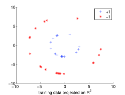
Refer to caption
Refer to caption
Refer to caption
Refer to caption
Refer to caption
Refer to caption
Figure 2: Nonlinear classification simulation with σ=3𝜎3\sigma=3. (a) Training data projected on the first two dimensions, (b) Training data projected on two S-EDRs derived by SGL. (c)Training data projected on first two ESFs derived by GL. (d) Test data projected on the first two dimensions. (e) Test data projected on two S-EDRs derived by SGL. (f) Test data projected on first two ESFs derived by GL.
Refer to caption
Refer to caption
Refer to caption
Refer to caption
Refer to caption
Refer to caption
Figure 3: Nonlinear classification simulation with σ=3𝜎3\sigma=3 (continued). (a) RKHS norm of empirical gradient derived by SGL. (b) S-EGCM for first 10 dimension. (c) Eigenvalues of S-EGCM. (d) RKHS norm of empirical gradient derived by GL, (e) EGCM for first 10 dimension. (f) Eigenvalues of EGCM.

We generated several datasets with different noise levels by varying σ𝜎\sigma from 0.10.10.1 to 333. SGL correctly selected x1superscript𝑥1x^{1} and x2superscript𝑥2x^{2} as the important variables for all cases we tested. Furthermore, SGL also generated two S-EDRs that captured the underlying data structure for all these cases (Figure 2). It is important to emphasize that the two S-EDRs generated by SGL are the only two features the algorithm can possibly obtain, since the derived S-EGCM are supported on a 2×2222\times 2 matrix. As a result, both of the derived S-EDRs are linear combinations of the first two variables. By contrast, using the gradient learning method (GL) reported in [25], the first two returned dimension reduction directions (called ESFs) are shown to be able to capture the correct underlying structure only when σ<0.7𝜎0.7\sigma<0.7. In addition, the derived ESFs are linear combinations of all 200200200 original variables instead of only two variables as in S-EDRs. Figure 2(b,e) shows the training data and the test data projected on the derived two S-EDRs for a dataset with large noise (σ=3𝜎3\sigma=3). Comparing to the data projected on the first two dimensions (Figure 2(a)(d)), the derived S-EDRs preserves the structure of the original data. In contrast, the gradient learning algorithm without sparsity constraint performed much poorer (Figure 2(c)(f)).

To explain why SGL performed better than GL without sparsity constraint, we plotted the norms of the derived empirical gradients from both methods in Figure 3. Note that although the norms of partial derivatives of unimportant variables derived from the method without sparsity constraint are small, they are not exactly zero. As a result, all variables contributed and, consequently, introduced noise to the empirical gradient covariance matrix (Figure 3(e)(f)).

We also tested LASSO for this artificial data set, and not surprisingly it failed to identify the right variables in all cases we tested. We omit the details here.

6.3 Leukemia classification

Next we apply SGL to do variable selection and dimension reduction on gene expression data. A gene expression data typically consists of the expression values of tens of thousands of mRNAs from a small number of samples as measured by microarrays. Because of the large number of genes involved, the variable selection step becomes especially important both for the purpose of generating better prediction models, and also for elucidating biological mechanisms underlying the data.

The gene expression data we will use is a widely studied dataset, consisting of the measurements of 712971297129 genes from 727272 acute leukemia samples [44]. The samples are labeled with two leukemia types according to the precursor of the tumor cells - one is called acute lymphoblastic leukemia (ALL), and the other one is called acute myelogenous leukemia (AML). The two tumor types are difficult to distinguish morphologically, and the gene expression data is used to build a classifier to classify these two types.

Among 727272 samples, 383838 are training data and 343434 are test data. We coded the type of leukaemia as a binary response variable y𝑦y, with 111 and 11-1 representing ALL and AML respectively. The variables in the training samples {𝐱i}i=138superscriptsubscriptsubscript𝐱𝑖𝑖138\{\mathbf{x}_{i}\}_{i=1}^{38} are normalized to be zero mean and unit length for each gene. The test data are similarly normalized, but only using the empirical mean and variance of the training data.

We applied three methods (SGL, GL and LASSO) to the dataset to select variables and extract the dimension reduction directions. To compare the performance of the three methods, we used linear SVM to build a classifier based on the variables or features returned by each method, and evaluated the classification performance using both leave-one-out (LOO) error on the training data and the testing error. To implement SGL, the bandwidth parameter s𝑠s is chosen to be half of the median of the pairwise distances of the sampling points, and 𝒦(𝐱,𝐲)=𝐱𝐲𝒦𝐱𝐲𝐱𝐲\mathcal{K}(\mathbf{x},\mathbf{y})=\mathbf{x}\mathbf{y}. The regularization parameters for the three methods are all chosen according to their prediction power measured by leave-one-out error.

Table 2:

Summary of the Leukemia classification results

Method SGL(variable selection) SGL(S-EDRs) GL(ESFs) Linear SVM LASSO
number of variables or features 106106106 111 666 712971297129(all) 33
leave one out error (LOO) 0/380380/38 0/380380/38 0/380380/38 3/383383/38 1/381381/38
test errors 0/340340/34 0/340340/34 2/342342/34 2/342342/34 1/341341/34

Table 2 shows the results of the three methods. We implemented two SVM classifiers for SGL using either only the variables or the features returned by SGL. Both classifiers are able to achieve perfect classification for both leave-one-out and testing samples. The performance of SGL is better than both GL and LASSO, although only slightly. All three methods performed significantly better than the SVM classifier built directly from the raw data.

In addition to the differences in prediction performance, we note a few other observations. First, SGL selects more genes than LASSO, which likely reflects the failure of LASSO to choose genes with nonlinear relationships with the response variable, as we illustrated in our first example. Second, The S-EDRs derived by SGL are linear combinations of 106106106 selected variables rather than all original variables as in the case of ESFs derived by GL. This is a desirable property since an important goal of the gene expression analysis is to identify regulatory pathways underlying the data, e.g. those distinguishing the two types of tumors. By associating only a small number of genes, S-EDRs provide better and more manageable candidate pathways for further experimental testing.

7 Discussion

Variable selection and dimension reduction are two common strategies for high-dimensional data analysis. Although many methods have been proposed before for variable selection or dimension reduction, few methods are currently available for simultaneous variable selection and dimension reduction. In this work, we described a sparse gradient learning algorithm that integrates automatic variable selection and dimension reduction into the same optimization framework. The algorithm can be viewed as a generalization of LASSO from linear to non-linear variable selection, and a generalization of the OPG method for learning EDR directions from a non-regularized to regularized estimation. We showed that the integrated framework offers several advantages over the previous methods by using both simulated and real-world examples.

The SGL method can be refined by using an adaptive weight function rather than a fixed one as in our current implementation. The weight function ωi,jssuperscriptsubscript𝜔𝑖𝑗𝑠\omega_{i,j}^{s} is used to measure the distance between two sample points. If the data are lying in a lower dimensional space, the distance would be more accurately captured by using only variables related to the lower dimensional space rather than all variables. One way to implement this is to calculate the distance using only selected variables. Note that the forward-backward splitting algorithm eliminates variables at each step of the iteration. We can thus use an adaptive weight function that calculates the distances based only on selected variables returned after each iteration. More specifically, let 𝒮(k)={i:(𝐜~i)(k)20}superscript𝒮𝑘conditional-set𝑖subscriptnormsuperscriptsuperscript~𝐜𝑖𝑘20\mathcal{S}^{(k)}=\{i:\|(\widetilde{\mathbf{c}}^{i})^{(k)}\|_{2}\neq 0\} represent the variables selected after iteration k𝑘k. An adaptive approach is to use l𝒮(k)(xilxjl)2subscript𝑙superscript𝒮𝑘superscriptsuperscriptsubscript𝑥𝑖𝑙superscriptsubscript𝑥𝑗𝑙2\sum_{l\in\mathcal{S}^{(k)}}(x_{i}^{l}-x_{j}^{l})^{2} to measure the distance 𝐱i𝐱j2superscriptnormsubscript𝐱𝑖subscript𝐱𝑗2\|\mathbf{x}_{i}-\mathbf{x}_{j}\|^{2} after iteration k𝑘k.

An interesting area for future research is to extend SGL for semi-supervised learning. In many applications, it is often much easier to obtain unlabeled data with a larger sample size u>>nmuch-greater-than𝑢𝑛u>>n. Most natural (human or animal) learning seems to occur in semi-supervised settings [45]. It is possible to extend SGL for the semi-supervised learning along several directions. One way is to use the unlabeled data 𝒳={𝐱i}i=n+1n+u𝒳superscriptsubscriptsubscript𝐱𝑖𝑖𝑛1𝑛𝑢\mathcal{X}=\{\mathbf{x}_{i}\}_{i=n+1}^{n+u} to control the approximate norm of f𝑓\vec{f} in some Sobolev spaces and introduce a semi-supervised learning algorithm as

f𝒵,𝒳,λ,μsubscript𝑓𝒵𝒳𝜆𝜇\displaystyle\vec{f}_{\mathcal{Z},\mathcal{X},\lambda,\mu} =\displaystyle= argminfKp{1n2i,j=1nωi,js(yiyj+f(𝐱i)(𝐱j𝐱i))2\displaystyle\arg\min_{\vec{f}\in{\cal H}_{K}^{p}}\bigg{\{}\frac{1}{n^{2}}\sum_{i,j=1}^{n}\omega_{i,j}^{s}\big{(}y_{i}-y_{j}+\vec{f}(\mathbf{x}_{i})\cdot(\mathbf{x}_{j}-\mathbf{x}_{i})\big{)}^{2}
+μ(n+u)2i,j=1n+uWi,jf(𝐱i)f(𝐱j)2(p)2+λfK},\displaystyle+\frac{\mu}{(n+u)^{2}}\sum_{i,j=1}^{n+u}W_{i,j}\|\vec{f}(\mathbf{x}_{i})-\vec{f}(\mathbf{x}_{j})\|^{2}_{\ell^{2}(\mathbb{R}^{p})}+\lambda\|\vec{f}\|_{K}\bigg{\}},

where fK=i=1pfiKsubscriptnorm𝑓𝐾superscriptsubscript𝑖1𝑝subscriptnormsuperscript𝑓𝑖𝐾\|\vec{f}\|_{K}=\sum_{i=1}^{p}\|f^{i}\|_{K}, Wi,jsubscript𝑊𝑖𝑗{W_{i,j}} are edge weights in the data adjacency graph, μ𝜇\mu is another regularization parameter and often satisfies λ=o(μ)𝜆𝑜𝜇\lambda=o(\mu). In order to make the algorithm efficiency, we can use truncated weight in implementation as done in section 6.1.

The regularization term i,j=1n+uWi,jf(𝐱i)f(𝐱j)2(p)2superscriptsubscript𝑖𝑗1𝑛𝑢subscript𝑊𝑖𝑗subscriptsuperscriptnorm𝑓subscript𝐱𝑖𝑓subscript𝐱𝑗2superscript2superscript𝑝\sum_{i,j=1}^{n+u}W_{i,j}\|\vec{f}(\mathbf{x}_{i})-\vec{f}(\mathbf{x}_{j})\|^{2}_{\ell^{2}(\mathbb{R}^{p})} is mainly motivated by the recent work of M. Belkin and P. Niyogi [45]. In that paper, they have introduced a regularization term i,j=1n+uWi,j(f(𝐱i)f(𝐱j))2superscriptsubscript𝑖𝑗1𝑛𝑢subscript𝑊𝑖𝑗superscript𝑓subscript𝐱𝑖𝑓subscript𝐱𝑗2\sum_{i,j=1}^{n+u}W_{i,j}(f(\mathbf{x}_{i})-f(\mathbf{x}_{j}))^{2} for semi-supervised regression and classification problems. The term i,j=1n+uWi,j(f(𝐱i)f(𝐱j))2superscriptsubscript𝑖𝑗1𝑛𝑢subscript𝑊𝑖𝑗superscript𝑓subscript𝐱𝑖𝑓subscript𝐱𝑗2\sum_{i,j=1}^{n+u}W_{i,j}(f(\mathbf{x}_{i})-f(\mathbf{x}_{j}))^{2} is well-known to be related to graph Laplacian operator. It is used to approximate 𝐱f2𝑑ρX(𝐱)subscript𝐱superscriptnormsubscript𝑓2differential-dsubscript𝜌𝑋𝐱\int_{\mathbf{x}\in\mathcal{M}}\|\nabla_{\mathcal{M}}f\|^{2}d\rho_{X}(\mathbf{x}), where \mathcal{M} is a compact submanifold which is the support of marginal distribution ρX(𝐱)subscript𝜌𝑋𝐱\rho_{X}(\mathbf{x}), and subscript\nabla_{\mathcal{M}} is the gradient of f𝑓f defined on \mathcal{M} [34]. Intuitively, 𝐱f2𝑑ρX(𝐱)subscript𝐱superscriptnormsubscript𝑓2differential-dsubscript𝜌𝑋𝐱\int_{\mathbf{x}\in\mathcal{M}}\|\nabla_{\mathcal{M}}f\|^{2}d\rho_{X}(\mathbf{x}) is a smoothness penalty corresponding to the probability distribution. The idea behind 𝐱f2𝑑ρX(𝐱)subscript𝐱superscriptnormsubscript𝑓2differential-dsubscript𝜌𝑋𝐱\int_{\mathbf{x}\in\mathcal{M}}\|\nabla_{\mathcal{M}}f\|^{2}d\rho_{X}(\mathbf{x}) is that it reflects the intrinsic structure of ρX(𝐱)subscript𝜌𝑋𝐱\rho_{X}(\mathbf{x}). Our regularization term i,j=1n+uWi,jf(𝐱i)f(𝐱j)2(p)2superscriptsubscript𝑖𝑗1𝑛𝑢subscript𝑊𝑖𝑗subscriptsuperscriptnorm𝑓subscript𝐱𝑖𝑓subscript𝐱𝑗2superscript2superscript𝑝\sum_{i,j=1}^{n+u}W_{i,j}\|\vec{f}(\mathbf{x}_{i})-\vec{f}(\mathbf{x}_{j})\|^{2}_{\ell^{2}(\mathbb{R}^{p})} is a corresponding vector form of i,j=1n+uWi,j(f(𝐱i)f(𝐱j))2superscriptsubscript𝑖𝑗1𝑛𝑢subscript𝑊𝑖𝑗superscript𝑓subscript𝐱𝑖𝑓subscript𝐱𝑗2\sum_{i,j=1}^{n+u}W_{i,j}(f(\mathbf{x}_{i})-f(\mathbf{x}_{j}))^{2} in [45]. The regularization framework of the SGL for semi-supervised learning can thus be viewed as a generalization of this previous work.

References

  • Guyon and Ellsseeff [2003] I. Guyon and A. Ellsseeff. An introduction to variable and feature selection. Journal of Machine Learning Research, 3:1157–1182, 2003.
  • Weston et al. [2003] J. Weston, A. Elisseff, B. Schölkopf, and M. Tipping. Use of the zero norm with linear models and kernel methods. Journal of Machine Learning Research, 3:1439–1461, 2003.
  • Dhillon et al. [2003] I. S. Dhillon, S. Mallela, and R. Kumar. A divisive information theoretic feature clustering algorithm for text classification. Journal of Machine Learning Research, 3:1265–1287, 2003.
  • Tibshirani [1996] Robert Tibshirani. Regression shrinkage and selection via the lasso. J. Roy. Statist. Soc. Ser. B, 58(1):267–288, 1996.
  • Zou and Hastie [2005] H. Zou and T. Hastie. Regularization and variable selection via the elastic net. J. R. Stat. Soc. Ser. B Stat. Methodol., 67(2):301–320, 2005.
  • Efron et al. [2004] B. Efron, T. Hastie, I. Johnstone, and R. Tibshirani. Least angle regression. Ann. Statist., 32(2):407–499, 2004. With discussion, and a rejoinder by the authors.
  • Lin and Zhang [2006] Y. Lin and H. H. Zhang. Component selection and smoothing in multivariate nonparametric regression. Ann. Statist., 34(5):2272–2297, 2006. ISSN 0090-5364. 10.1214/009053606000000722.
  • Belkin and Niyogi [2003] M. Belkin and P. Niyogi. Laplacian eigenmaps for dimensionality reduction and data representation. Neural Compput., 15(6):1373–1396, 2003.
  • Zou et al. [2006] H. Zou, T. Hastie, and R. Tibshirani. Sparse principal component analysis. J. Comput. Graph. Statist., 15(2):265–286, 2006.
  • Mackey [2009] L. Mackey. Deflation methods for sparse pca. Advances in Neural Information Processing Systems, 21:1017–1024, 2009.
  • Roweis and Saul [2000] S.T. Roweis and L.K. Saul. Nonlinear dimensionality reduction by locally linear embedding. Science, 290(5500):2323–2326, 2000.
  • Tenenbaum et al. [2000] J.B. Tenenbaum, V. Silva, and J.C. Langford. A global geometric framework for nonlinear dimensionality reduction. Science, 290(5500):2319–2323, 2000.
  • Donoho and Grimes [2003] D.L. Donoho and C. Grimes. Hessian eigenmaps: Locally linear embedding techniques for high-dimensional data. Proc. Natl. Acad. Sci., 100(10):5591–5596, 2003.
  • Xia et al. [2002] Y. Xia, H. Tong, W. K. Li, and L.-X. Zhu. An adaptive estimation of dimension reduction space. J. R. Stat. Soc. Ser. B Stat. Methodol., 64(3):363–410, 2002. 10.1111/1467-9868.03411.
  • Li [1991] Ker-Chau Li. Sliced inverse regression for dimension reduction. J. Amer. Statist. Assoc., 86(414):316–342, 1991. With discussion and a rejoinder by the author.
  • Li [1992] Ker-Chau Li. On principal Hessian directions for data visualization and dimension reduction: another application of Stein’s lemma. J. Amer. Statist. Assoc., 87(420):1025–1039, 1992.
  • Cook and Yin [2001] R. Dennis Cook and Xiangrong Yin. Dimension reduction and visualization in discriminant analysis. Aust. N. Z. J. Stat., 43(2):147–199, 2001. 10.1111/1467-842X.00164. With a discussion by A. H. Welsh, Trevor Hastie, Mu Zhu, S. J. Sheather, J. W. McKean, Xuming He and Wing-Kam Fung and a rejoinder by the authors.
  • Li et al. [2005] B. Li, H. Zha, and F. Chiaromonte. Contour regression: A general approach to dimension reduction. Ann. Statist., pages 1580–1616, 2005.
  • Hristache et al. [2001] M. Hristache, A. Juditsky, and V. Spokoiny. Structure adaptive approach for dimension reduction. Ann. Statist., 29(6):1537–1566, 2001.
  • Samarov [1993] Alexander M. Samarov. Exploring regression structure using nonparametric functional estimation. J. Amer. Statist. Assoc., 88(423):836–847, 1993.
  • Fukumizu et al. [2009] K. Fukumizu, F. R. Bach, and M. I. Jordan. Kernel dimension reduction in regression. Ann. Statist., 37(4):1871–1905, 2009. 10.1214/08-AOS637.
  • Mukherjee and Zhou [2006] S. Mukherjee and D. X. Zhou. Learning coordinate covariances via gradients. Journal of Machine Learning Research, 7:519–549, 2006.
  • Mukherjee and Wu [2006] S. Mukherjee and Q. Wu. Estimation of gradients and coordinate covariation in classification. Journal of Machine Learning Research, 7:2481–2514, 2006.
  • Guyon et al. [2002] I. Guyon, J. Weston, S. Barnhill, and V. Vapnik. Gene selection for cancer classification using support vector machines. Machine Learning, 46(1):389–422, 2002.
  • Mukherjee et al. [2010] S. Mukherjee, Q. Wu, and D.X. Zhou. Learning gradients on manifolds. Bernoulli, 2010.
  • Lafferty and Wasserman [2008] J. Lafferty and L. Wasserman. Rodeo: sparse, greedy nonparametric regression. Ann. Statist., 36(1):28–63, 2008. ISSN 0090-5364. 10.1214/009053607000000811.
  • Aronszajn [1950] N. Aronszajn. Theory of reproducing kernels. Trans. Amer. Math. Soc., 68:337–404, 1950.
  • Donoho [1995] D. L. Donoho. De-noising by soft-thresholding. IEEE Trans. Inform. Theory, 41(3):613–627, 1995.
  • Daubechies et al. [2004] Ingrid Daubechies, Michel Defrise, and Christine De Mol. An iterative thresholding algorithm for linear inverse problems with a sparsity constraint. Comm. Pure Appl. Math., 57(11):1413–1457, 2004. 10.1002/cpa.20042.
  • Donoho [2006] D. L. Donoho. Compressed sensing. IEEE Trans. Inform. Theory, 52(4):1289–1306, 2006.
  • Vapnik [1998] V. N. Vapnik. Statistical learning theory. Adaptive and Learning Systems for Signal Processing, Communications, and Control. John Wiley & Sons Inc., New York, 1998. A Wiley-Interscience Publication.
  • Micchelli and Pontil [2005] Charles A. Micchelli and M. Pontil. On learning vector-valued functions. Neural Comput., 17(1):177–204, 2005. 10.1162/0899766052530802.
  • Ye and Zhou [2008] Gui-Bo Ye and Ding-Xuan Zhou. Learning and approximation by Gaussians on Riemannian manifolds. Adv. Comput. Math., 29(3):291–310, 2008.
  • Do Carmo and Flaherty [1992] M.P. Do Carmo and F. Flaherty. Riemannian geometry. Birkhauser, 1992.
  • Golub and Van Loan [1989] G. H. Golub and C. F. Van Loan. Matrix computations. Johns Hopkins University Press, 1989.
  • Zhang [2004] T. Zhang. Statistical behavior and consistency of classification methods based on convex risk minimization. Ann. Statist., 32(1):56–85, 2004. ISSN 0090-5364. 10.1214/aos/1079120130.
  • McDiarmid [1989] Colin McDiarmid. On the method of bounded differences. Surveys in combinatorics, 141:148–188, 1989.
  • van der Vaart and Wellner [1996] A. W. van der Vaart and Jon A. Wellner. Weak convergence and empirical processes. Springer Series in Statistics. Springer-Verlag, New York, 1996. With applications to statistics.
  • Schölkopf and Smola [2002] B. Schölkopf and A.J. Smola. Learning with kernels: Support vector machines, regularization, optimization, and beyond. MIT press, 2002.
  • Langford et al. [2009] J. Langford, L. Li, and T. Zhang. Sparse online learning via truncated gradient. In D. Koller, D. Schuurmans, Y. Bengio, and L. Bottou, editors, Advances in Neural Information Processing Systems 21, pages 905–912. MIT, 2009.
  • Cai et al. [2008] J.-F. Cai, R. H. Chan, and Z. Shen. A framelet-based image inpainting algorithm. Appl. Comput. Harmon. Anal., 24(2):131–149, 2008.
  • Combettes and Wajs [2005] Patrick L. Combettes and Valérie R. Wajs. Signal recovery by proximal forward-backward splitting. Multiscale Model. Simul., 4(4):1168–1200 (electronic), 2005. 10.1137/050626090.
  • Hiriart-Urruty and Lemaréchal [1993] J.B. Hiriart-Urruty and C. Lemaréchal. Convex Analysis and Minimization Algorithms. Springer-Verlag, Berlin, 1993.
  • Golub et al. [1999] T. R. Golub, D. K. Slonim, P. Tamayo, C. Huard, M. Gaasenbeek, J. P. Mesirov, H. Coller, M. L. Loh, J. R. Downing, M. A. Caligiuri, C. D. Bloomfield, and E. S. Lander. Molecular classification of cancer: Class discovery and class prediction by gene expression monitoring. Science, 286(5439):531–537, 1999.
  • Belkin et al. [2006] M. Belkin, P. Niyogi, and V. Sindhwani. Manifold regularization: A geometric framework for learning from labeled and unlabeled examples. Journal of Machine Learning Research, 7:2434, 2006.