Fast ABC-Boost for Multi-Class Classification

Abstract

Abc-boost is a new line of boosting algorithms for multi-class classification, by utilizing the commonly used sum-to-zero constraint. To implement abc-boost, a base class must be identified at each boosting step. Prior studies used a very expensive procedure based on exhaustive search for determining the base class at each boosting step. Good testing performance of abc-boost (implemented as abc-mart and abc-logitboost) on a variety of datasets was reported.

For large datasets, however, the exhaustive search strategy adopted in prior abc-boost algorithms can be too prohibitive. To overcome this serious limitation, this paper suggests a heuristic by introducing Gaps when computing the base class during training. That is, we update the choice of the base class only for every $G$ boosting steps (i.e., $G=1$ in prior studies). We test this idea on large datasets (Covertype and Poker) as well as datasets of moderate size. Our preliminary results are very encouraging. On the large datasets, when $G\leq 100$ (or even larger), there is essentially no loss of test accuracy compared to using $G=1$. On the moderate datasets, no obvious loss of test accuracy is observed when $G\leq 20\sim 50$. Therefore, aided by this heuristic of using gaps, it is promising that abc-boost will be a practical tool for accurate multi-class classification.

1 Introduction

This study focuses on significantly improving the computational efficiency of abc-boost, a new line of boosting algorithms recently proposed for multi-class classification [8, 9]. Boosting [11, 3, 4, 1, 12, 6, 10, 5, 2] has been successful in machine learning and industry practice.

In prior studies, abc-boost has been implemented as abc-mart [8] and abc-logitboost [9]. Therefore, for completeness, we first provide a review of logitboost [6] and mart (multiple additive regression trees) [5].

1.1 Data Probability Model and Loss Function

We denote a training dataset by $\{y_{i},\mathbf{x}_{i}\}_{i=1}^{N}$, where $N$ is the number of feature vectors (samples), $\mathbf{x}_{i}$ is the $i$th feature vector, and $y_{i}\in\{0,1,2,...,K-1\}$ is the $i$th class label, where $K\geq 3$ in multi-class classification.

Both logitboost [6] and mart [5] can be viewed as generalizations to the classical logistic regression, which models class probabilities $p_{i,k}$ as

$$p_{i,k}=\mathbf{Pr}\left(y_{i}=k|\mathbf{x}_{i}\right)=\frac{e^{F_{i,k}(\mathbf{x_{i}})}}{\sum_{s=0}^{K-1}e^{F_{i,s}(\mathbf{x_{i}})}}.$$ (1)

While logistic regression simply assumes $F_{i,k}(\mathbf{x}_{i})=\beta^{\text{T}}_{k}\mathbf{x}_{i}$,  logitboost and mart adopt the flexible “additive model,” which is a function of $M$ terms:

$$F^{(M)}(\mathbf{x})=\sum_{m=1}^{M}\rho_{m}h(\mathbf{x};\mathbf{a}_{m}),$$ (2)

where $h(\mathbf{x};\mathbf{a}_{m})$, the base (weak) learner, is typically a regression tree. The parameters, $\rho_{m}$ and $\mathbf{a}_{m}$, are learned from the data, by maximizing the joint likelihood, which is equivalent to minimizing the following negative log-likelihood loss function:

$$L=\sum_{i=1}^{N}L_{i},\hskip 28.90755ptL_{i}=-\sum_{k=0}^{K-1}r_{i,k}\log p_{i,k}$$ (3)

where $r_{i,k}=1$ if $y_{i}=k$ and $r_{i,k}=0$ otherwise. For identifiability, $\sum_{k=0}^{K-1}F_{i,k}=0$, i.e., the sum-to-zero constraint, is typically adopted [6, 5, 14, 7, 13, 16, 15].

1.2 The (Robust) Logitboost and Mart Algorithms

The logitboost algorithm [6] builds the additive model (2) by a greedy stage-wise procedure, using a second-order (diagonal) approximation of the loss function (3). The standard practice is to implement logitboost using regression trees. The mart algorithm [5] is a creative combination of gradient descent and Newton’s method, by using the first-order information of the loss function (3) to construct the trees and using both the first- & second-order derivatives to determine the values of the terminal nodes.

Therefore, both logitboost and mart require the first two derivatives of the loss function (3) with respective to the function values $F_{i,k}$. [6, 5] used the following derivatives:

$$\frac{\partial L_{i}}{\partial F_{i,k}}=-\left(r_{i,k}-p_{i,k}\right),\hskip 21.68121pt\frac{\partial^{2}L_{i}}{\partial F_{i,k}^{2}}=p_{i,k}\left(1-p_{i,k}\right).$$ (4)

The recent work named robust logitboost [9] is a numerically stable implementation of logitboost. [9] unified logitboost and mart by showing that their difference lies in the tree-split criterion for constructing the regression trees at each boosting iteration.

1.2.1 Tree-Split Criteria for (Robust) Logitboost and Mart

Consider $N$ weights $w_{i}$, and $N$ response values $z_{i}$, $i=1$ to $N$, which are assumed to be ordered according to the ascending order of the corresponding feature values. The tree-split procedure is to find the index $s$, $1\leq s<N$, such that the weighted square error (SE) is reduced the most if split at $s$. That is, we seek the $s$ to maximize the gain:

$$Gain(s)=SE_{T}-(SE_{L}+SE_{R})$$

$$= \sum_{i=1}^{N}(z_{i}-\bar{z})^{2}w_{i}-\left[\sum_{i=1}^{s}(z_{i}-\bar{z}_{L})^{2}w_{i}+\sum_{i=s+1}^{N}(z_{i}-\bar{z}_{R})^{2}w_{i}\right]$$ (5)

where

$$\bar{z}=\frac{\sum_{i=1}^{N}z_{i}w_{i}}{\sum_{i=1}^{N}w_{i}},\hskip 10.84006pt\bar{z}_{L}=\frac{\sum_{i=1}^{s}z_{i}w_{i}}{\sum_{i=1}^{s}w_{i}},\hskip 10.84006pt\bar{z}_{R}=\frac{\sum_{i=s+1}^{N}z_{i}w_{i}}{\sum_{i=s+1}^{N}w_{i}}.$$

[9] showed the expression (5) can be simplified to be

$$Gain(s)= \frac{\left[\sum_{i=1}^{s}z_{i}w_{i}\right]^{2}}{\sum_{i=1}^{s}w_{i}}+\frac{\left[\sum_{i=s+1}^{N}z_{i}w_{i}\right]^{2}}{\sum_{i=s+1}^{N}w_{i}}-\frac{\left[\sum_{i=1}^{N}z_{i}w_{i}\right]^{2}}{\sum_{i=1}^{N}w_{i}}.$$ (6)

For logitboost, [6] used the weights $w_{i}=p_{i,k}(1-p_{i,k})$ and the responses $z_{i}=\frac{r_{i,k}-p_{i,k}}{p_{i,k}(1-p_{i,k})}$, i.e.,

$$LogitGain(s)= \frac{\left[\sum_{i=1}^{s}\left(r_{i,k}-p_{i,k}\right)\right]^{2}}{\sum_{i=1}^{s}p_{i,k}(1-p_{i,k})}+\frac{\left[\sum_{i=s+1}^{N}\left(r_{i,k}-p_{i,k}\right)\right]^{2}}{\sum_{i=s+1}^{N}p_{i,k}(1-p_{i,k})}-\frac{\left[\sum_{i=1}^{N}\left(r_{i,k}-p_{i,k}\right)\right]^{2}}{\sum_{i=1}^{N}p_{i,k}(1-p_{i,k})}.$$ (7)

For mart, [5] used the weights $w_{i}=1$ and the responses $z_{i,k}=r_{i,k}-p_{i,k}$, i.e.,

$$MartGain(s)=\frac{1}{s}\left[\sum_{i=1}^{s}\left(r_{i,k}-p_{i,k}\right)\right]^{2}+\frac{1}{N-s}\left[\sum_{i=s+1}^{N}\left(r_{i,k}-p_{i,k}\right)\right]^{2}-\frac{1}{N}\left[\sum_{i=1}^{N}\left(r_{i,k}-p_{i,k}\right)\right]^{2}.$$ (8)

1.2.2 The Robust Logitboost Algorithm

1: $F_{i,k}=0$, $p_{i,k}=\frac{1}{K}$, $k=0$ to $K-1$, $i=1$ to $N$
2: For $m=1$ to $M$ Do
3:     For $k=0$ to $K-1$ Do
4:      $\left\{R_{j,k,m}\right\}_{j=1}^{J}=J$-terminal node regression tree from $\{r_{i,k}-p_{i,k},\ \ \mathbf{x}_{i}\}_{i=1}^{N}$, with weights $p_{i,k}(1-p_{i,k})$ as in (7)
5:       $\beta_{j,k,m}=\frac{K-1}{K}\frac{\sum_{\mathbf{x}_{i}\in R_{j,k,m}}r_{i,k}-p_{i,k}}{\sum_{\mathbf{x}_{i}\in R_{j,k,m}}\left(1-p_{i,k}\right)p_{i,k}}$
6:       $F_{i,k}=F_{i,k}+\nu\sum_{j=1}^{J}\beta_{j,k,m}1_{\mathbf{x}_{i}\in R_{j,k,m}}$
7:     End
8:    $p_{i,k}=\exp(F_{i,k})/\sum_{s=0}^{K-1}\exp(F_{i,s})$
9: End

Algorithm 1 Robust logitboost, which is very similar to the mart algorithm [5], except for Line 4.

Alg. 1 describes robust logitboost using the tree-split criterion (7). In Line 6, $\nu$ is the shrinkage parameter and is normally set to be $\nu\leq 0.1$. Note that after trees are constructed, the values of the terminal nodes are computed by

$$\frac{\sum_{node}z_{i,k}w_{i,k}}{\sum_{node}w_{i,k}}=\frac{\sum_{node}r_{i,k}-p_{i,k}}{\sum_{node}p_{i,k}(1-p_{i,k})},$$ (9)

which explains Line 5 of Alg. 1.

1.2.3 The Mart Algorithm

The mart algorithm only uses the first derivative to construct the tree. Once the tree is constructed, [5] applied a one-step Newton update to obtain the values of the terminal nodes. Interestingly, this one-step Newton update yields exactly the same equation as (9). In other words, (9) is interpreted as weighted average in logitboost but it is interpreted as the one-step Newton update in mart. Thus, the mart algorithm is similar to Alg. 1; we only need to change Line 4, by replacing (7) with (8).

2 Review Adaptive Base Class Boost (ABC-Boost)

Developed by [8], the abc-boost algorithm consists of the following two components:

1. Using the widely-used sum-to-zero constraint [6, 5, 14, 7, 13, 16, 15] on the loss function, one can formulate boosting algorithms only for $K-1$ classes, by using one class as the base class.

2. At each boosting iteration, adaptively select the base class according to the training loss (3). [8] suggested an exhaustive search strategy.

[8] derived the derivatives of (3) under the sum-to-zero constraint. Without loss of generality, we can assume that class 0 is the base class. For any $k\neq 0$,

$$\frac{\partial L_{i}}{\partial F_{i,k}}=\left(r_{i,0}-p_{i,0}\right)-\left(r_{i,k}-p_{i,k}\right),$$ (10)

$$\frac{\partial^{2}L_{i}}{\partial F_{i,k}^{2}}=p_{i,0}(1-p_{i,0})+p_{i,k}(1-p_{i,k})+2p_{i,0}p_{i,k}.$$ (11)

[8] combined the idea of abc-boost with mart to develop abc-mart, which achieved good performance in multi-class classification. More recently, [9] developed abc-logitboost by combining abc-boost with robust logitboost.

2.1 ABC-LogitBoost and ABC-Mart

Alg. 2 presents abc-logitboost, using the derivatives in (10) and (11) and the same exhaustive search strategy proposed in [8]. Compared to Alg. 1, abc-logitboost differs from (robust) logitboost in that they use different derivatives and abc-logitboost needs an additional loop to select the base class at each boosting iteration.

1: $F_{i,k}=0$,   $p_{i,k}=\frac{1}{K}$,    $k=0$ to $K-1$,  $i=1$ to $N$
2: For $m=1$ to $M$ Do
3:     For $b=0$ to $K-1$, Do
4:       For $k=0$ to $K-1$, $k\neq b$, Do
5:          $\left\{R_{j,k,m}\right\}_{j=1}^{J}=J$-terminal node regression tree from $\{-(r_{i,b}-p_{i,b})+(r_{i,k}-p_{i,k}),\ \ \mathbf{x}_{i}\}_{i=1}^{N}$ with
:           weights $p_{i,b}(1-p_{i,b})+p_{i,k}(1-p_{i,k})+2p_{i,b}p_{i,k}$, in Sec. 1.2.1.
6:          $\beta_{j,k,m}=\frac{\sum_{\mathbf{x}_{i}\in R_{j,k,m}}-(r_{i,b}-p_{i,b})+(r_{i,k}-p_{i,k})}{\sum_{\mathbf{x}_{i}\in R_{j,k,m}}p_{i,b}(1-p_{i,b})+p_{i,k}\left(1-p_{i,k}\right)+2p_{i,b}p_{i,k}}$

7:          $g_{i,k,b}=F_{i,k}+\nu\sum_{j=1}^{J}\beta_{j,k,m}1_{\mathbf{x}_{i}\in R_{j,k,m}}$
8:       End
9:       $g_{i,b,b}=-\sum_{k\neq b}g_{i,k,b}$
10:       $q_{i,k}=\exp(g_{i,k,b})/\sum_{s=0}^{K-1}\exp(g_{i,s,b})$
11:       $L^{(b)}=-\sum_{i=1}^{N}\sum_{k=0}^{K-1}r_{i,k}\log\left(q_{i,k}\right)$
12:     End
13:     $B(m)=\underset{b}{\text{argmin}}\ \ L^{(b)}$
14:     $F_{i,k}=g_{i,k,B(m)}$
15:    $p_{i,k}=\exp(F_{i,k})/\sum_{s=0}^{K-1}\exp(F_{i,s})$
16: End

Algorithm 2 Abc-logitboost using the exhaustive search strategy for the base class, as suggested in [8]. The vector $B$ stores the base class numbers.

Again, abc-logitboost differs from abc-mart only in the tree-split procedure (Line 5 in Alg. 2).

2.2 Why Does the Choice of Base Class Matter?

[9] used the Hessian matrix, to demonstrate why the choice of the base class matters.

The chose of the base class matters because of the diagonal approximation; that is, fitting a regression tree for each class at each boosting iteration. To see this, we can take a look at the Hessian matrix, for $K=3$. Using the original logitboost/mart derivatives (4), the determinant of the Hessian matrix is

$$\left|\begin{array}[]{ccc}\frac{\partial^{2}L_{i}}{\partial p_{0}^{2}}&\frac{\partial^{2}L_{i}}{\partial p_{0}p_{1}}&\frac{\partial^{2}L_{i}}{\partial p_{0}p_{2}}\\ \frac{\partial^{2}L_{i}}{\partial p_{1}p_{0}}&\frac{\partial^{2}L_{i}}{\partial p_{1}^{2}}&\frac{\partial^{2}L_{i}}{\partial p_{1}p_{2}}\\ \frac{\partial^{2}L_{i}}{\partial p_{2}p_{0}}&\frac{\partial^{2}L_{i}}{\partial p_{2}p_{1}}&\frac{\partial^{2}L_{i}}{\partial p_{2}^{2}}\end{array}\right|=\left|\begin{array}[]{ccc}p_{0}(1-p_{0})&-p_{0}p_{1}&-p_{0}p_{2}\\ -p_{1}p_{0}&p_{1}(1-p_{1})&-p_{1}p_{2}\\ -p_{2}p_{0}&-p_{2}p_{1}&p_{2}(1-p_{2})\\ \end{array}\right|={0}$$ (18)

as expected, because there are only $K-1$ degrees of freedom. A simple fix is to use the diagonal approximation [6, 5]. In fact, when trees are used as the weak learner, it seems one must use the diagonal approximation.

Now, consider the derivatives (10) and (11) used in abc-mart and abc-logitboost. This time, when $K=3$ and $k=0$ is the base class, we only have a 2 by 2 Hessian matrix, whose determinant is

$$\left|\begin{array}[]{cc}\frac{\partial^{2}L_{i}}{\partial p_{1}^{2}}&\frac{\partial^{2}L_{i}}{\partial p_{1}p_{2}}\\ \frac{\partial^{2}L_{i}}{\partial p_{2}p_{1}}&\frac{\partial^{2}L_{i}}{\partial p_{2}^{2}}\end{array}\right|=\left|\begin{array}[]{cc}p_{0}(1-p_{0})+p_{1}(1-p_{1})+2p_{0}p_{1}&p_{0}-p_{0}^{2}+p_{0}p_{1}+p_{0}p_{2}-p_{1}p_{2}\\ p_{0}-p_{0}^{2}+p_{0}p_{1}+p_{0}p_{2}-p_{1}p_{2}&p_{0}(1-p_{0})+p_{2}(1-p_{2})+2p_{0}p_{2}\\ \end{array}\right|$$ (23)

$$= p_{0}p_{1}+p_{0}p_{2}+p_{1}p_{2}-p_{0}p_{1}^{2}-p_{0}p_{2}^{2}-p_{1}p_{2}^{2}-p_{2}p_{1}^{2}-p_{1}p_{0}^{2}-p_{2}p_{0}^{2}+6p_{0}p_{1}p_{2},$$

which is non-zero and is in fact independent of the choice of the base class (even though we assume $k=0$ as the base in this example). In other words, the choice of the base class would not matter if the full Hessian is used.

However, because we will have to use diagonal approximation in order to construct trees at each iteration, the choice of the base class will matter.

2.3 Datasets Used for Testing Fast ABC-Boost

We will test fast abc-boost using a subset of the datasets in [9], as listed in Table 1. Because the computational cost of abc-boost is not a concern for small datasets, this study focuses on fairly large datasets (Covertype and Poker) as well as datasets of moderate size (Mnist10k and M-Image).

Table 1: Datasets

dataset	$K$	# training	# test	# features
Covertype290k	7	290506	290506	54
Poker525k	10	525010	500000	25
Poker275k	10	275010	500000	25
Mnist10k	10	10000	60000	784
M-Image	10	12000	50000	784

2.4 Review the Detailed Experiment Results of ABC-Boost on Mnist10k and M-Image

For these two datasets, [9] experimented with every combination of $J\in\{4,6,8,10,12,14,16,18,20,24,30,40,50\}$ and $\nu\in\{0.04,0.06,0.08,0.1\}$. The four boosting algorithms were trained till the training loss (3) was close to the machine accuracy, to exhaust the capacity of the learners, for reliable comparisons, up to $M=10000$ iterations. Since no obvious overfitting was observed, the test mis-classification errors at the last iterations were reported.

Table 2 and Table 3 present the test mis-classification errors, which verify the consistent improvements of (A) abc-logitboost over (robust) logitboost, (B) abc-logitboost over abc-mart, (C) (robust) logitboost over mart, and (D) abc-mart over mart. The tables also verify that the performances are not too sensitive to the parameters ($J$ and $\nu$).

Table 2: Mnist10k. Upper table: The test mis-classification errors of mart and abc-mart (bold numbers). Bottom table: The test errors of logitboost and abc-logitboost (bold numbers)

	mart	abc-mart
	$\nu=0.04$	$\nu=0.06$	$\nu=0.08$	$\nu=0.1$
$J=4$	3356 3060	3329 3019	3318 2855	3326 2794
$J=6$	3185 2760	3093 2626	3129 2656	3217 2590
$J=8$	3049 2558	3054 2555	3054 2534	3035 2577
$J=10$	3020 2547	2973 2521	2990 2520	2978 2506
$J=12$	2927 2498	2917 2457	2945 2488	2907 2490
$J=14$	2925 2487	2901 2471	2877 2470	2884 2454
$J=16$	2899 2478	2893 2452	2873 2465	2860 2451
$J=18$	2857 2469	2880 2460	2870 2437	2855 2454
$J=20$	2833 2441	2834 2448	2834 2444	2815 2440
$J=24$	2840 2447	2827 2431	2801 2427	2784 2455
$J=30$	2826 2457	2822 2443	2828 2470	2807 2450
$J=40$	2837 2482	2809 2440	2836 2447	2782 2506
$J=50$	2813 2502	2826 2459	2824 2469	2786 2499
	logitboost	abc-logit
	$\nu=0.04$	$\nu=0.06$	$\nu=0.08$	$\nu=0.1$
$J=4$	2936 2630	2970 2600	2980 2535	3017 2522
$J=6$	2710 2263	2693 2252	2710 2226	2711 2223
$J=8$	2599 2159	2619 2138	2589 2120	2597 2143
$J=10$	2553 2122	2527 2118	2516 2091	2500 2097
$J=12$	2472 2084	2468 2090	2468 2090	2464 2095
$J=14$	2451 2083	2420 2094	2432 2063	2419 2050
$J=16$	2424 2111	2437 2114	2393 2097	2395 2082
$J=18$	2399 2088	2402 2087	2389 2088	2380 2097
$J=20$	2388 2128	2414 2112	2411 2095	2381 2102
$J=24$	2442 2174	2415 2147	2417 2129	2419 2138
$J=30$	2468 2235	2434 2237	2423 2221	2449 2177
$J=40$	2551 2310	2509 2284	2518 2257	2531 2260
$J=50$	2612 2353	2622 2359	2579 2332	2570 2341

Table 3: M-Image. Upper table: The test mis-classification errors of mart and abc-mart (bold numbers). Bottom table: The test of logitboost and abc-logitboost (bold numbers)

	mart	abc-mart
	$\nu=0.04$	$\nu=0.06$	$\nu=0.08$	$\nu=0.1$
$J=4$	6536 5867	6511 5813	6496 5774	6449 5756
$J=6$	6203 5471	6174 5414	6176 5394	6139 5370
$J=8$	6095 5320	6081 5251	6132 5141	6220 5181
$J=10$	6076 5138	6104 5100	6154 5086	6332 4983
$J=12$	6036 4963	6086 4956	6104 4926	6117 4867
$J=14$	5922 4885	6037 4866	6018 4789	5993 4839
$J=16$	5914 4847	5937 4806	5940 4797	5883 4766
$J=18$	5955 4835	5886 4778	5896 4733	5814 4730
$J=20$	5870 4749	5847 4722	5829 4707	5821 4727
$J=24$	5816 4725	5766 4659	5785 4662	5752 4625
$J=30$	5729 4649	5738 4629	5724 4626	5702 4654
$J=40$	5752 4619	5699 4636	5672 4597	5676 4660
$J=50$	5760 4674	5731 4667	5723 4659	5725 4649
	logitboost	abc-logit
	$\nu=0.04$	$\nu=0.06$	$\nu=0.08$	$\nu=0.1$
$J=4$	5837 5539	5852 5480	5834 5408	5802 5430
$J=6$	5473 5076	5471 4925	5457 4950	5437 4919
$J=8$	5294 4756	5285 4748	5193 4678	5187 4670
$J=10$	5141 4597	5120 4572	5052 4524	5049 4537
$J=12$	5013 4432	5016 4455	4987 4416	4961 4389
$J=14$	4914 4378	4922 4338	4906 4356	4895 4299
$J=16$	4863 4317	4842 4307	4816 4279	4806 4314
$J=18$	4762 4301	4740 4255	4754 4230	4751 4287
$J=20$	4714 4251	4734 4231	4693 4214	4703 4268
$J=24$	4676 4242	4610 4298	4663 4226	4638 4250
$J=30$	4653 4351	4662 4307	4633 4311	4643 4286
$J=40$	4713 4434	4724 4426	4760 4439	4768 4388
$J=50$	4763 4502	4795 4534	4792 4487	4799 4479

3 Fast ABC-Boost

Recall that, in abc-boost, the base class must be identified at each boosting iteration. The exhaustive search strategy used in [8, 9] is obviously very expensive. In this paper, our main contribution is a proposal for speeding up abc-boost by introducing Gaps when selecting the base class. Again, we illustrate our strategy using abc-mart and abc-logitboost, which are only two implementations of abc-boost so far.

Assuming $M$ boosting iterations, the computation cost of mart and logitboost is $O(KM)$. However, the computation cost of abc-mart and abc-logitboost $O\left(K(K-1)M\right)$, which can be prohibitive.

The reason we need to select the base class is because we have to use the the diagonal approximation in order to fit a regression separately for each class at every boosting iteration. Based on this insight, we really do not have to re-compute the base class for every iteration. Instead, we only compute the base class for every $G$ steps, where $G$ is the gap and $G=1$ means we select the base class for every iteration.

After introducing gaps, the computation cost of fast abc-boost is reduced to $O\left(K(K-1)\frac{M}{G}+\left(M-\frac{M}{G}\right)(K-1)\right)$. One can verify that when $G=(K-1)$, the cost of fast abc-boost is at most twice as the cost of logitboost. As we increases $G$ more, the additional computational overhead of fast abc-boost further diminishes.

The parameter $G$ can be viewed as a new tuning parameter. Our experiments (in the following subsections) illustrate that when $G\leq 100$ (or $G\leq 20\sim 50$), there would be no obvious loss of test accuracies in large datasets (or moderate datasets).

3.1 Experiments on Large Datasets, Poker525k, Poker275k, and Covertype290k

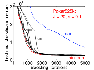
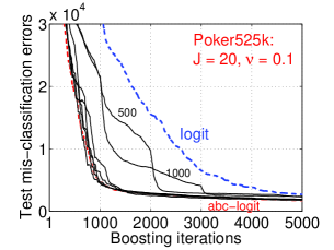
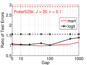
As presented in [9], on the Poker dataset, abc-boost achieved very remarkable improvements over mart and logitboost, especially when the number of boosting iterations was not too large. In fact, even at $M=5000$ iterations, the mis-classification error of mart (or (robust) logitboost) is 3 times (or 1.5 times) as large as the error of abc-mart (or abc-logitboost); see the rightmost panel of Figure 1.

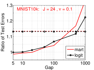
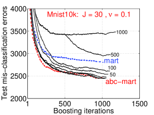
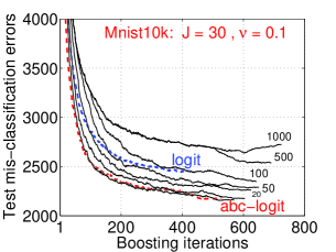
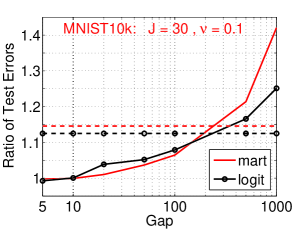
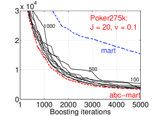
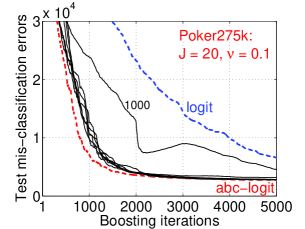
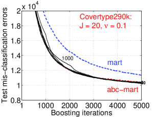
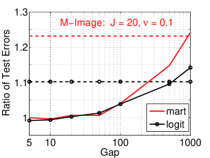
Figure 1: Poker525k      Left panel: test mis-classification errors of abc-mart (with $G=1,5,10,20,50,100,500,1000$) and mart, for all boosting iterations up to $M=5000$ steps. We only label the curves which are distinguishable (in this case $G=500$ and 1000). Middle panel: test mis-classification errors of abc-logitboost and (robust) logitboost. Note that, at $M=5000$, the test error of abc-logitboost is significantly smaller than the test error of logitboost, even though, due to the scaling issue, the difference may be less obvious in the figure. Right panel: the ratios of test errors, i.e., mart over abc-mart and logitboost over abc-logitboost, at the last (i.e., $M=5000$) boosting iteration. The two dashed horizontal lines represent the test error ratios at $G=1$ (i.e., the original abc-boost). Note that a ratio of 1.5 (or even 3) should be considered extremely large for classification tasks.

For all datasets, we experiment with $G=1$ (i.e., the original abc-boost), $5,10,20,50,100,500,1000$. As shown in Figure 1, using fast abc-boost with $G\leq 100$, there is no obvious loss of test accuracies on Poker525k. In fact, using abc-mart, even with $G=1000$, there is only very little loss of accuracy.

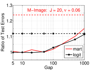
Note that it is possible for fast abc-boost to achieve smaller test errors than abc-boost; for example, the ratios of test errors in the right panel of Figure 1 may be below 1.0. This interesting phenomenon is not surprising. After all, $G$ can be viewed as tuning parameter and using $G>1$ may have some regularization effect because that would be less greedy.

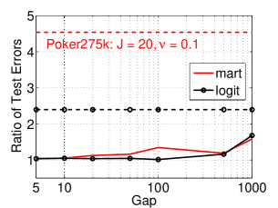
Figure 2 presents the test error results on Poker275k, which are very similar to the results on Poker525k.

Figure 2: Poker275k.       See the caption of Figure 1 for explanations.

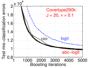
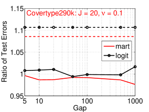
Figure 3 presents the test error results on Covertype290k. For this dataset, even with $G=1000$, we notice essentially no loss of test accuracies.

Figure 3: Covertype290k

3.2 Experiments on Moderate Datasets, M-Image and Mnist10k

The situation is somewhat different on datasets that are not too large. Recall, for these two datasets, we terminate the training if the training loss (3) is to close to the machine accuracy, up to $M=10000$ iterations.

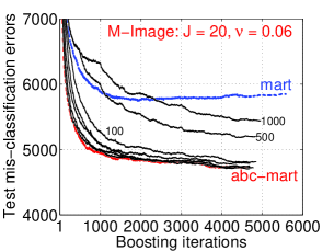
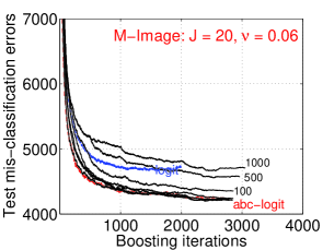
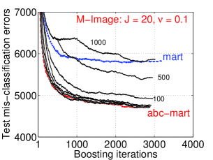
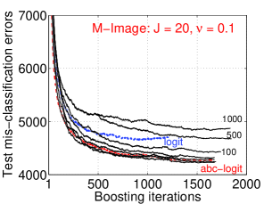
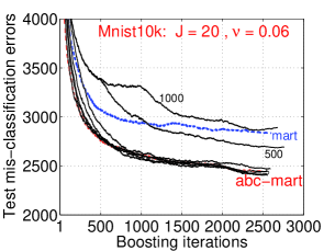
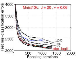
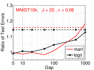
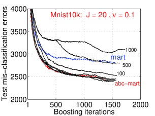
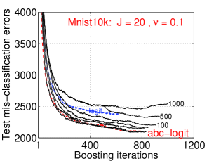
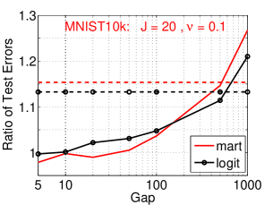
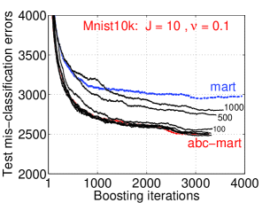
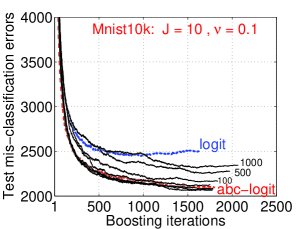
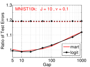
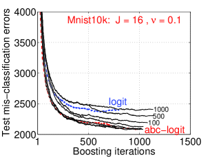
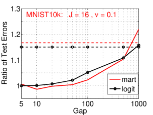
Figure 4 and Figure 5 show that, on M-Image and Mnist10k, using fast abc-boost with $G>50$ can result in non-negligible loss of test accuracies compared to using $G=1$. When $G$ is too large, e.g., $G=1000$, it is possible that fast abc-boost may produce even larger test errors than mart or logitboost.

Figure 4 and Figure 5 report the test errors for $J=20$ and two shrinkages, $\nu=0.06,0.1$. It seems that, at the same $G$, using smaller $\nu$ produces slightly better results.

Figure 4: M-Image      See the caption of Figure 1 for explanations.

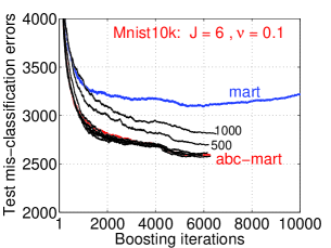
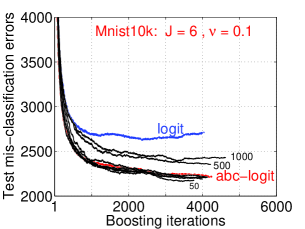
Figure 5: Mnist10k      See the caption of Figure 1 for explanations.

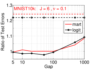
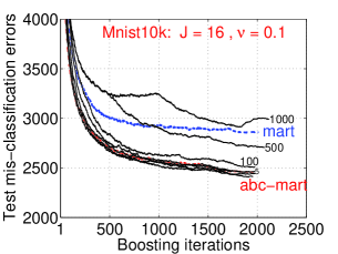
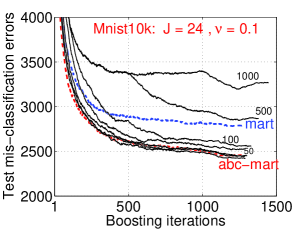
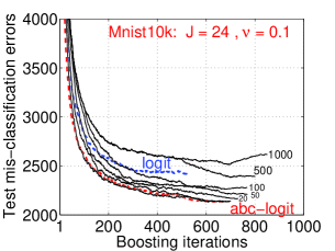
The above experiments always use $J=20$, which seems to be a reasonable number of terminal tree nodes for large or moderate datasets. Nevertheless, it would be interesting to experiment with other $J$ values. Figure 6 presents the results on the Mnist10k dataset, for $J=6,10,16,20,24,30$.

When $J$ is small (e.g., $J=6$), using $G$ as large as 100 results in almost no loss of test accuracies. However, when $J$ is large (e.g., $J=30$), even with $G=50$ may produce obviously less accurate results compared to $G=1$.

Figure 6: Mnist10k

4 Conclusion

This study proposes fast abc-boost to significantly improve the training speed of abc-boost, which suffered from serious problems of computational efficiency. Abc-boost is a new line of boosting algorithms for improving multi-class classification, which was implemented as abc-mart and abc-logitboost in prior studies. Abc-boost requires that a base class must be identified at each boosting iteration. The computation of the base class was based on an expensive exhaustive search strategy in prior studies.

With fast abc-boost, we only need to update the choice of the base class once for every $G$ iterations, where $G$ can be viewed as Gaps and used as an additional tuning parameter. Our experiments on fairly large datasets show that the test errors are not sensitive to the choice of $G$, even with $G=100$ or 1000. For datasets of moderate size, our experiments show that, when $G\leq 20\sim 50$, there would be no obvious loss of test accuracies compared to the original abc-boost algorithms (i.e., $G=1$).

These preliminary results are very encouraging. We expect fast abc-boost will be a practical tool for accurate multi-class classification.

References

• [1] Peter Bartlett, Yoav Freund, Weeย Sun Lee, and Robertย E. Schapire. Boosting the margin: a new explanation for the effectiveness of voting methods. The Annals of Statistics, 26(5):1651โ€“1686, 1998.
• [2] Peter Bรผhlmann and Bin Yu. Boosting with the L2 loss: Regression and classification. Journal of the American Statistical Association, 98(462):324โ€“339, 2003.
• [3] Yoav Freund. Boosting a weak learning algorithm by majority. Inf. Comput., 121(2):256โ€“285, 1995.
• [4] Yoav Freund and Robertย E. Schapire. A decision-theoretic generalization of on-line learning and an application to boosting. J. Comput. Syst. Sci., 55(1):119โ€“139, 1997.
• [5] Jeromeย H. Friedman. Greedy function approximation: A gradient boosting machine. The Annals of Statistics, 29(5):1189โ€“1232, 2001.
• [6] Jeromeย H. Friedman, Trevorย J. Hastie, and Robert Tibshirani. Additive logistic regression: a statistical view of boosting. The Annals of Statistics, 28(2):337โ€“407, 2000.
• [7] Yoonkyung Lee, Yiย Lin, and Grace Wahba. Multicategory support vector machines: Theory and application to the classification of microarray data and satellite radiance data. Journal of the American Statistical Association, 99(465):67โ€“81, 2004.
• [8] Ping Li. Abc-boost: Adaptive base class boost for multi-class classification. In ICML, pages 625โ€“632, Montreal, Canada, 2009.
• [9] Ping Li. Robust logitboost and adaptive base class (abc) logitboost. In UAI, 2010.
• [10] Liew Mason, Jonathan Baxter, Peter Bartlett, and Marcus Frean. Boosting algorithms as gradient descent. In NIPS, 2000.
• [11] Robert Schapire. The strength of weak learnability. Machine Learning, 5(2):197โ€“227, 1990.
• [12] Robertย E. Schapire and Yoram Singer. Improved boosting algorithms using confidence-rated predictions. Machine Learning, 37(3):297โ€“336, 1999.
• [13] Ambuj Tewari and Peterย L. Bartlett. On the consistency of multiclass classification methods. Journal of Machine Learning Research, 8:1007โ€“1025, 2007.
• [14] Tong Zhang. Statistical analysis of some multi-category large margin classification methods. Journal of Machine Learning Research, 5:1225โ€“1251, 2004.
• [15] Jiย Zhu, Hui Zou, Saharon Rosset, and Trevor Hastie. Multi-class adaboost. Statistics and Its Interface, 2(3):349โ€“360, 2009.
• [16] Hui Zou, Jiย Zhu, and Trevor Hastie. New multicategory boosting algorithms based on multicategory fisher-consistent losses. The Annals of Applied Statistics, 2(4):1290โ€“1306, 2008.