Reconciling alternate methods for the determination of charge distributions: A probabilistic approach to high-dimensional least-squares approximations.

Abstract

We propose extensions and improvements of the statistical analysis of distributed multipoles (SADM) algorithm put forth by Chipot et al in [6] for the derivation of distributed atomic multipoles from the quantum-mechanical electrostatic potential. The method is mathematically extended to general least-squares problems and provides an alternative approximation method in cases where the original least-squares problem is computationally not tractable, either because of its ill-posedness or its high-dimensionality. The solution is approximated employing a Monte Carlo method that takes the average of a random variable defined as the solutions of random small least-squares problems drawn as subsystems of the original problem. The conditions that ensure convergence and consistency of the method are discussed, along with an analysis of the computational cost in specific instances.

MSC numbers: 65C05, 93E24, 41A45, 41A63

Keywords: Least-squares approximation, Monte Carlo methods, high dimensional problems.

1 Introduction

In the realm of the molecular modeling of complex chemical systems, atom-centered multipole distributions constitute a popular route to simplify the description of intricate electron densities. Streamlined down to their most rudimentary representation, these densities are generally mimicked in macromolecular force fields by simple point charges, from which, in the context of molecular simulations, Coulomb interactions can be rapidly evaluated. Whereas nuclear charges are clearly centered onto the constituent atoms, the electron charge distribution extends over the entire molecular system. As a result, in sharp contrast with the higher-order multipole moments of a neutral molecule, which, strictly speaking, are quantum-mechanical observables, atomic charges cannot be defined univocally, in an equally rigorous fashion. They ought to be viewed instead as a convenient construct, the purpose of which is to reduce the complexity of molecular charge distributions by means of compact sets of parameters providing a useful, albeit naive framework to localize specific interactions onto atomic sites.

The ambiguous nature of atom-centered charges has, therefore, prompted the development of alternative paths towards their determination [8]. The choice of the numerical scheme ought to be dictated by three prevalent criteria, namely (i) the computational cost of the derivation, (ii) the ease of implementation within the framework of a physical model and (iii) the ability of the point-charge model to reproduce properties of interest with the desired accuracy. Under a number of circumstances, crude atomic charges determined through inexpensive calculations are shown to be adequate. In other, more common scenarios, for instance, in molecular simulations of complex chemical systems, the accurate description of the electrostatic interactions at play can be of paramount importance. The atomic charges utilized in these simulations are by and large derived from quantum-mechanical calculations carried out at a reasonably high level of theory, which in many cases, can be appreciably expensive. In the vast majority of popular potential energy functions, point-charge models are derived quantum-mechanically, following, in a nutshell, two distinct philosophies. On the one hand, the numerical simulations of condensed phases imposes that solute-solvent interactions be described as accurately as possible. Accordingly, in macromolecular force fields like Charmm [16], the atomic charges are determined based on a series of independent quantum-mechanical calculations featuring different relative positions of a solvent molecule around the solute. On the other hand, the electrostatic potential can be viewed as the fingerprint of the molecule, the accurate representation of which guarantees a reliable description of intermolecular interactions. In potential energy functions like Amber [9], point charges are derived from the molecular electrostatic potential, exploiting the fact that the latter is a quantum-mechanical observable readily accessible from the wave function.

In their seminal article, Cox and Williams [10] proposed an attractive approach, whereby sets of atom-centered charges can be easily derived on the basis of a single-point quantum-mechanical calculation. The electrostatic potential is evaluated on a grid of $M$ points lying around the molecule of interest, outside the van der Waals envelope of the latter. Restricting the multipole expansion of the electrostatic potential to the monopole term, the charges borne by the $n$ atomic sites of the molecule are determined by minimizing the root-mean square deviation between the reference, quantum-mechanical quantity and its zeroth-order approximation — i.e. $q_{i}T_{ki}^{00}$, where $T_{ki}^{00}=\|x_{i}-x_{k}\|^{-1}$, is the potential created at point $k$ by atomic site $i$. In its pioneering form, the algorithm handled the least-squares problem iteratively. Chirlian and Francl subsequently proposed to resort to a non-iterative numerical scheme [7], which obviates the need for initial guesses and solves the overdetermined system of linear equations through matrix inversion. This route for the derivation of point-charge models can be generalized in a straightforward fashion to higher-order multipoles.

The success of potential-derived charges stems in large measure from their ease of computation and the demonstration for a host of chemical systems that they are able to reproduce with an appreciable accuracy a variety of physical properties. This success is, however, partially clouded by one noteworthy shortcoming of the method — point charges borne by atoms buried in the molecule cannot be determined unambiguously from a rudimentary least-squares fitting procedure. Symptomatically, for those molecular systems, in which the contribution of the subset of buried atoms to the electrostatic potential is ill-defined, the derived charges are in apparent violation with the commonly accepted rules of electronegativity differences, e.g. a C^δ-—Cl^δ+ bond polarity in carbon tetrachloride, in lieu of the intuitive C^δ+—Cl^δ-. Bayly et al. tackled this issue through the introduction of hyperbolic penalty functions in their fitting procedure [3]. Arguably enough, this numerical scheme addresses the symptom rather than its actual cause. As was commented on by Francl et al. in the light of singular-value-decomposition analyses [13], the matrices of the least-squares problem are rank deficient, to the extent that statistically valid charges cannot be assigned univocally to the selected set of atoms in the molecule.

To delve further into this issue, Chipot et al. proposed an alternative algorithm coined statistical analysis of distributed multipoles (SADM) [6], wherein atom-centered multipoles are also derived from the quantum-mechanical electrostatic potential, yet following a somewhat different pathway than the conventional least-squares scheme. Instead of solving directly the $n\times M$ overdetermined system of linear equations, for instance through matrix inversion, a subset of $n$ points is drawn amongst the $M$ points of the grid and the corresponding $n\times n$ system of linear equations is solved. This procedure, referred to as an experiment, is repeated with different subsets of grid points, from whence probability distributions are obtained for the series of multipoles being sought. Strictly speaking, each probability distribution ought to be determined from C${}_{M}^{n}$ independent experiments. On account of the computational burden, however — viz. typically, for a molecule formed by ten atoms and a grid of 2,000 points sampling the three-dimensional space around it, this would imply solving approximately 2.76 $\times$ 10²⁶ systems of linear equations — only 3–5 $\times$ 10⁵ independent experiments are performed, which has proven heuristically to be appropriate.

The mathematical description of this problem is the following: denoting by $(q_{j})_{j=1}^{n}$ the unknown charges borne by the $n$ particles, and by $\gamma_{j}(x)=\|x-x_{j}\|^{-1}$, the electrostatic potential associated with each $x_{j}\in\mathbb{R}^{3}$, the least square problem consists in finding the minimum $(q_{j})_{j=1}^{n}\in\mathbb{R}^{n}$ of the function

$$\mathbb{R}^{n}\ni a\mapsto\sum_{i=1}^{M}|f(y_{i})-\sum_{j=1}^{n}a_{j}\gamma_{j}(y_{i})|^{2},$$ (1.1)

where $(y_{j})_{j=1}^{M}\in\mathbb{R}^{3M}$ are the coordinates of the $M$ external points. Here $f(y_{j})$ stands for the approximation of the electrostatic potential at $y_{j}$ obtained by quantum-mechanical calculations.

Instead of solving directly the problem (1.1), the SADM consists in drawing $n$ points $y^{(i)}$ amongst the $M$ points $y_{j}$, solve the $n\times n$ problem $f(y^{(i)})=\sum_{j=1}^{n}\gamma_{j}(y^{(i)})a_{j}$, $i=1,\ldots,n$ in the least squares sense and subsequently plot the distribution of each $a_{j}$. In [6], Chipot et al. notice that the latter are Cauchy-like distributions (with seemingly infinite expectation) centered around the exact solution of the original least-squares problem. Note that this method not only provides a numerical approximation of the solution, but also a global statistical distribution that reflects the accuracy of the physical model being utilized.

Interestingly enough, it turns out that this kind of approach can be extended to many situations arising in computational mathematics and physics. The principle of the SADM algorithm is in fact very general, and can be adapted to derive efficient algorithms that are robust with the dimension of the underlying space of approximation. This in turn provides new numerical methods of practical interest for high dimensional approximation problems, where traditional least-squares methods are impossible to implement, either because of the high dimensionality or the ill-posedness of the least-squares problem.

The goal of the present contribution is twofold:

• Introduce a general mathematical framework, and analyze the consistency, convergence and cost of the proposed algorithms in an abstract setting and in specific situations where calculations can be made explicit (Wishart or subgaussian distributions). The main outcome is that the subsystems drawn from the original system have to be chosen rectangular and not square (as initially proposed in the SADM method) to yield convergent and efficient algorithms. In other words, instead of drawing $n\times n$ subsystems, we will show that in many cases of applications, it is more interesting to draw $n\times n+2$ or $n\times 2n$ subsystems in order to control the expectation and variance of the distribution.

• Apply these results to revisit and improve the SADM method. This is mainly achieved in Section 5 by considering a simple, three-point charge model of water.

2 Mathematical setting

Let us now describe more precisely the problematic.

2.1 General least-squares problems

Let $(\Omega,\mu)$ be a probability space $\Omega$ equipped with a probability measure $\mu$. For a given arbitrary function $f\in\mathrm{L}^{2}(\Omega)$ and $n$ given functions $\gamma_{j}(x)\in\mathrm{L}^{2}(\Omega)$, $j=1,\ldots,n$ all taking values in $\mathbb{R}$, we consider the problem of approximating $f(x)$ by a linear combination of the functions $\gamma_{j}(x)$, $j=1,\ldots,n$.

Ideally, we would like to solve the problem of finding $\alpha=(\alpha_{j})_{j=1}^{n}\in\mathbb{R}^{n}$, minimizing the function

$$\mathbb{R}^{n}\ni a\mapsto\|f(x)-\sum_{j=1}^{n}a_{j}\gamma_{j}(x)\|\left.\vphantom{T_{j_{0}}^{0}}\!\!\right._{\mathrm{L}^{2}(\Omega)}^{2}.$$ (2.1)

The actual quality of the least-squares approximation is given by the size of the residue $\|\rho(\alpha)\|\left.\vphantom{T_{j_{0}}^{0}}\!\!\right._{\mathrm{L}^{2}(\Omega)}$ where for $a=(a_{j})_{j=1}^{n}\in\mathbb{R}^{n}$,

$$\rho(a)(x)=f(x)-\sum_{j=1}^{n}a_{j}\gamma_{j}(x).$$ (2.2)

Many minimization problems arising in mathematics and in physics can be stated under this form, for instance:

• $\Omega=[a,b]^{n}$ with two real numbers $a$ and $b>a$, and equipped with the measure $\mathrm{d}\mu(x)=(b-a)^{-n}\mathrm{d}x$ where $\mathrm{d}x$ is the Lebesgue measure on $\mathbb{R}^{n}$. Taking $\gamma:\Omega\to\mathbb{R}^{n+1}$ defined by $\gamma_{i}(x)=x_{i}$ for all $i\in\{1,\ldots,n\}$ and $\gamma_{n+1}\equiv 1$, the problem is equivalent to finding $\beta\in\mathbb{R}$ and $\alpha\in\mathbb{R}^{n}$ minimizing the function

  $$\|f(x)-\beta-\langle\alpha,x\rangle\|\left.\vphantom{T_{j_{0}}^{0}}\!\!\right._{\mathrm{L}^{2}([a,b]^{n})}^{2}$$

  where $\langle\,\cdot\,,\cdot\,\rangle$ is the standard Euclidean product in $\mathbb{R}^{n}$. This is nothing else than a multivariate linear interpolation.

  Similarly, any polynomial approximation problem in $\mathrm{L}^{2}([a,b]^{n},\mu)$, where $\mu$ is a weight function, can be written in the form (2.1) by taking as $\gamma_{j}$ a basis of polynomials in dimension $n$.

• Taking $\Omega=\mathbb{R}^{n}$ equipped with a given $n$-dimensional Gaussian measure leads to many different situations: The approximation by Hermite functions in $\mathbb{R}^{n}$ if $\gamma_{j}$ are polynomials, the approximation of $f$ by Gaussian chirps signal [18] in the case where $\gamma_{j}(x)$ are oscillating functions of $x$, or alternatively approximation by Gaussian wavepackets functions [15] in the context of molecular dynamics.

• Consider $\Omega=\{1,\ldots,M\}$ with $M\gg n$ equipped with the uniform probability measure $M^{-1}\sum_{i=1}^{M}\delta_{i}$. In this case, an application $f$ is represented by a vector $b\in\mathbb{R}^{M}$, whereas $\gamma$ is represented by a matrix $A$ with $n$ columns and $M$ lines. The problem is then equivalent to the problem of finding $\alpha\in\mathbb{R}^{n}$ that minimizes

  $$\|A\alpha-b\|\left.\vphantom{T_{j_{0}}^{0}}\!\!\right._{2}^{2}$$

  where $\|\cdot\|\left.\vphantom{T_{j_{0}}^{0}}\!\!\right._{2}$ is the Euclidean norm on $\mathbb{R}^{M}$. This corresponds to the case described in (1.1).

• Consider $\Omega=\mathbb{R}^{n}\times\Omega^{\prime}$ equipped with the measure $\mu\otimes\nu$ where $\mu$ and $\nu$ are probability measures on $\mathbb{R}^{n}$ and $\Omega^{\prime}$ respectively. Taking $f(x,\omega^{\prime})=h(x)+X(\omega^{\prime})$ where $X(\omega^{\prime})$ is a given random variable on $\Omega^{\prime}$, and $\gamma_{j}(x,\omega^{\prime})=x_{j}$ for $j=1,\ldots,n$ yields the problem of minimizing

  $$\min_{\alpha\in\mathbb{R}^{n}}\mathbb{E}\Big{[}\|\langle\alpha,x\rangle-f(x,\omega^{\prime})\|\left.\vphantom{T_{j_{0}}^{0}}\!\!\right._{\mathrm{L}^{2}(\mathbb{R}^{n})}^{2}\Big{]}$$ (2.3)

  which corresponds to the linear regression of a function observed with some independent noise.

The problem (2.1) is equivalent to solving the linear equation

$$\langle\gamma,\gamma^{T}\rangle_{\mathrm{L}^{2}}\alpha=\langle\gamma,f\rangle_{\mathrm{L}^{2}}$$

where $\alpha=(\alpha_{i})_{i=1}^{n}$ and $\langle\gamma,\gamma^{T}\rangle_{\mathrm{L}^{2}}$ is the $n\times n$ matrix with coefficients $\langle\gamma_{i},\gamma_{j}\rangle_{\mathrm{L}^{2}}$, $i,j=1,\ldots,n$.

If the family $(\gamma_{i}(x))_{i=1}^{n}$ defines a full rank set of elements of $\mathrm{L}^{2}(\Omega)$, the matrix $\langle\gamma,\gamma^{T}\rangle_{\mathrm{L}^{2}}$ is invertible, and the solution of the previous equation reads

$$\alpha=\langle\gamma,\gamma^{T}\rangle_{\mathrm{L}^{2}}^{-1}\cdot\langle\gamma,f\rangle_{\mathrm{L}^{2}}.$$ (2.4)

Apart from specific situations, where, for instance, the $\gamma_{j}$ can be assumed orthogonal, the numerical approximation of (2.4) is extremely costly with respect to the dimension of $\Omega$ (see for instance [4]). Typically, discretizations of problems of the form $\mathbf{(a)}$ yields a problem of the form $\mathbf{(c)}$ with $m=N^{n}$ where $N$ is the number of interpolation points in $[a,b]$ needed to approximate the $\mathrm{L}^{2}$ integrals. For $n=30$, this method is not tractable in practice, even if $N=2$.

To avoid this curse of dimensionality, an alternative would consist in approximating the integrals in the formula (2.4) by using Monte Carlo methods. In large dimension, the matrix $\langle\gamma,\gamma^{T}\rangle_{\mathrm{L}^{2}}$ is, however, often ill-conditioned, and obtaining a correct approximation of the inverse of this matrix might require in practice a very large number of draws to minimize the error in the value of $\alpha$.

2.2 Principle of the algorithm

In this abstract mathematical setting, the principle lying behind the SADM method can be extended to the following: Retaining the idea of drawing subsystems of the original problem, we consider the following algorithm:

• Draw $m$ points $X^{(i)}$, $i=1,\ldots,m$ in $\Omega$ independent and identically distibuted (i.i.d.) with distribution $\mu$.

• Solve the $m\times n$ least-squares sub-problem by determining $\beta$ minimizing the function

  $$\mathbb{R}^{n}\ni\beta\mapsto\sum_{i=1}^{m}|f(X^{(i)})-\sum_{j=1}^{m}\beta_{j}\gamma_{j}(X^{(i)})|^{2}.$$ (2.5)

• Approximate the expectation $\bar{\beta}$ of the random variable $\beta$ by a Monte-Carlo method and analyse its distribution.

More precisely, we define $X:=(X^{(1)},\ldots,X^{(m)})$ and the functions $F:\Omega^{m}\to\mathbb{R}^{m}$ and $\Gamma:\Omega^{m}\to\mathscr{L}(\mathbb{R}^{m},\mathbb{R}^{n})$ by the formulae

$$\forall i=1,\ldots,m,\quad F_{i}(x^{(1)},\ldots,x^{(m)})=f(x^{(i)})$$ (2.6)

and

$$\forall i=1,\ldots,m,\quad\forall\,j=1,\ldots,n,\quad\Gamma_{ij}(x^{(1)},\ldots,x^{(m)})=\gamma_{j}(x^{(i)}).$$ (2.7)

The random vector $\beta$ then minimizes the function

$$\beta\mapsto\|F(X)-\Gamma(X)\beta\|\left.\vphantom{T_{j_{0}}^{0}}\!\!\right._{2}^{2},$$

where $\|\cdot\|\left.\vphantom{T_{j_{0}}^{0}}\!\!\right._{2}$ is the standard Euclidean norm on $\mathbb{R}^{m}$.

Under the assumption that $\Gamma^{T}(X)\Gamma(X)$ is invertible almost surely (a.s.),

$$\beta=R(X)F(X):=((\Gamma^{T}\Gamma)^{-1}\Gamma^{T})(X)F(X).$$ (2.8)

The expectation of $\beta$ is then given by the formula

$$\bar{\beta}:=\mathbb{E}\beta=\int_{\Omega^{m}}((\Gamma^{T}\Gamma)^{-1}\Gamma^{T}F)(x^{(1)},\ldots,x^{(m)})\,\mathrm{d}\mu(x^{(1)})\otimes\cdots\otimes\mathrm{d}\mu(x^{(m)}).$$ (2.9)

Our algorithm consists in using the Monte-Carlo method to compute the previous expectation: we approximate $\bar{\beta}$ by

$$\bar{\beta}_{N}=\frac{1}{N}\sum_{i=1}^{N}\beta_{i},$$ (2.10)

where $\beta_{i},i\geq 1$ are i.i.d. realizations of the random vector $\beta\in\mathbb{R}^{n}$, obtained by (2.8) from i.i.d. realizations of the random $n\times m$ matrix $\Gamma(X)$.

Of course, one expects that $\bar{\beta}$ should converge to the solution of the least square problem (2.4) when $m\rightarrow+\infty$. This indeed can be easily proved under the additional assumption that $f$ and $\gamma_{j}$, $1\leq j\leq n$ belong to $\mathrm{L}^{2}(\Omega)$. By the strong law of large numbers,

$$\frac{1}{m}(\Gamma(X)^{T}\Gamma(X))_{ij}=\frac{1}{m}\sum_{k=1}^{m}\gamma_{i}(X^{(k)})\gamma_{j}(X^{(k)})$$ (2.11)

converges $\mathbb{P}$-a.s. to $(\langle\gamma,\gamma^{T}\rangle_{\mathrm{L}^{2}})_{ij}$ when $m\rightarrow+\infty$. Similarly,

$$\frac{1}{m}(\Gamma(X)^{T}F(X))_{i}=\frac{1}{m}\sum_{k=1}^{m}\gamma_{i}(X^{(k)})f(X^{(k)})$$ (2.12)

converges $\mathbb{P}$-a.s. to $(\langle\gamma,f\rangle_{\mathrm{L}^{2}})_{i}$. Consequently, if the matrix $\langle\gamma,\gamma^{T}\rangle_{\mathrm{L}^{2}}$ is invertible,

$$\beta=\Big{(}\frac{1}{m}\Gamma^{T}(X)\Gamma(X)\Big{)}^{-1}\frac{1}{m}\Gamma(X)^{T}F(X)$$ (2.13)

converges $\mathbb{P}$-a.s. to $\alpha$ given by (2.4) when $m\rightarrow+\infty$.

However our goal is not to analyse more finely this convergence, as we are concerned with situations where the least square problem (2.1) is ill-posed or computationally unfeasible due to the high diemsnion of the problem. In the opposite, considering the case where $m$ is small in comparison with the dimension of $\Omega$ ($M$ in the case of SADM) should reduce the computational cost, provided that the efficiency of the Monte-Carlo approximation is good. To express the fact that we are in a regime where $m$ is small, we assume in the following that $\boldsymbol{m\leq Cn}$ for some constant $C$ (typically $m=n+2$ or $m=2n$ for practical applications).

Therefore, to make sure that the previous algorithm is efficient, we have to verify the following points:

• The random variable $\beta$ has finite expectation and variance. Here the bounds may depend on $n$, but not on the cardinal of $\Omega$ ($M$ in the SADM description above). This condition is crucial to ensure the convergence of a Monte-Carlo method and the approximability of $\bar{\beta}$. In addition, the smaller is the variance, the faster the Monte-Carlo approximation converges to $\bar{\beta}$.

• The average $\bar{\beta}$ is a good alternative to the solution of the original problem (2.1) in the sense that $\bar{\beta}-\alpha=\mathscr{O}(\|\rho(a)\|\left.\vphantom{T_{j_{0}}^{0}}\!\!\right.)$ where $\rho(a)$ is the residue (2.2). In other words, if $f$ is close to a linear combination of the functions $\gamma$ the residue will be small and the standard least-square approximation will be efficient. In this situation, $\bar{\beta}$ will also lead to a good approximation, and be close to the solution $\alpha$. On the other hand, when the residue is large, $\bar{\beta}$ and $\alpha$ may differ, but in this situation the approximation of $f$ by a linear combination of the functions of $\gamma$ is poor in any case.

In Section 3 we give various conditions that warrant the latter requirements. In particular, we study the consistency of the algorithm, give conditions ensuring the convergence of the Monte Carlo method, and analyze the computational cost. In the specific instance where $\Gamma(X)^{T}\Gamma(X)$ has the Wishart distribution, all computations can be made explicitly, and we obtain precise estimates and an optimal choice of the parameter $m$. The two values $m=n+2$ and $m=2n$ are of specific interest in this situation. In addition, we prove that the choice $m=n$ leads to a random variable $\beta$ with infinite expectation, which partly explains the Cauchy-like distributions observed in [6] with the SADM method.

2.3 The algorithm in the non-invertible case

In practice, the almost sure invertibility of $\Gamma^{T}(X)\Gamma(X)$ cannot be guaranteed — and obviously not for problems of the form $\mathbf{(c)}$, where all the random variables $X^{(1)},\ldots,X^{(m)}$ may be equal with positive probability.

In a more general setting, we, hence, restrict ourselves to realizations of $X$, such that matrix $\Gamma(X)$ is sufficiently well conditioned, in the following sense: Denoting by $s_{1}(\Gamma(X))$ the smallest eigenvalue of the symmetric positive matrix $\Gamma(X)^{T}\Gamma(X)$, we only consider realizations of $X$, such that $s_{1}(\Gamma(X))$ is greater than some threshold $\sigma$, which may depend on $n$ and $m$. In this case, rather than approximating (2.9), we will estimate the conditional expectation

$$\bar{\beta}^{\sigma}:=\mathbb{E}^{\sigma}\beta=\mathbb{E}[\,\beta\mid s_{1}(\Gamma(X))>\sigma\,]$$ (2.14)

by

$$\bar{\beta}_{N}^{\sigma}=\frac{1}{N}\sum_{i=1}^{N}\beta_{i}^{\sigma},$$ (2.15)

where the $\beta^{\sigma}_{i}$ are obtained from a sequence of i.i.d. realizations of the random vector $\beta\in\mathbb{R}^{n}$ in (2.8), from which have been removed all realizations such that $s_{1}(\Gamma(X))\leq\sigma$. Note that (2.10) is a particular case of (2.15) for $\sigma=0$, provided that $\mathbb{P}(s_{1}(\Gamma(X))=0)=0$.

Again, such a method will be of interest in terms of computational cost if $m$ is on the order of magnitude of $n$ (in all the applications considered herein, $m=n+2$ or $m=2n$ will be sufficient) and if $\mathbb{P}(s_{1}(\Gamma(X))>\sigma)$ is not too small — because drawing a realization of $X$ such that $s_{1}(\Gamma(X))>\sigma$ requires an average number $\mathbb{P}(s_{1}(\Gamma(X))>\sigma)^{-1}$ of realizations of $X$.

From the perspective of precision, this method will perform well if the variance of $\beta$ conditionally on $\{s_{1}(\Gamma(X))>\sigma\}$ has an appropriate behavior with respect to $n$ and $m$, and if $\bar{\beta}^{\sigma}$ defined in (2.14) provides a good approximation of the solution of the original least-squares problem.

The specific case where the $\Gamma(X)^{T}\Gamma(X)$ is not a.s. invertible is studied in Section 4, where we give various conditions that warrant the latter requirements. The instance where $\Gamma(X)$ has subgaussian entries (which covers the Wishart case mentionned above) is then studied in more details and leads again to optimal choices of $m$, $N$ and $\sigma$.

3 The invertible case

In all this section, we assume that the matrix $\Gamma(X)^{T}\Gamma(X)$ is a.s. invertible.

3.1 Preliminary results

Before studying the algorithm of Section 2.2, let us define for $q\in[2,+\infty]$

$$K_{q}(\Gamma):=\left[\mathbb{E}\,\frac{1}{s_{1}(\Gamma(X))^{\frac{q}{2}}}\right]^{\frac{2}{q}},$$ (3.1)

where $\Gamma(X)$ is the random matrix defined by (2.7) and with the usual convention that $K_{\infty}(\Gamma)=\|s_{1}(\Gamma(X))^{-1}\|_{\mathrm{L}^{\infty}}$. Note that $K_{q}(\Gamma)$ depends on $n$ and $m$.

The proof of the next lemma is given in Appendix A.

Lemma 3.1

Let $p\in[1,\infty]$ and $g\in\mathrm{L}^{p}(\Omega)$. Let us define the function $G$ from $g$ as $F$ is defined from $f$ in (2.6). Let also $R(X)$ be the random matrix defined in (2.8).

(a)

Assume that $K_{q}(\Gamma)<+\infty$ where $q$ is such that $q^{-1}+p^{-1}=1$. Then we have

$$\mathbb{E}\|R(X)G(X)\|\left.\vphantom{T_{j_{0}}^{0}}\!\!\right._{2}\leq\sqrt{n}m\sqrt{K_{q}(\Gamma)}\|g\|\left.\vphantom{T_{j_{0}}^{0}}\!\!\right._{\mathrm{L}^{p}(\Omega)}.$$ (3.2)

(b)

Assume that $p\in[2,\infty]$ and that $K_{q}(\Gamma)<+\infty$ where $q$ is such that $2q^{-1}+2p^{-1}=1$. Then we have

$$\mathbb{E}\|R(X)G(X)\|\left.\vphantom{T_{j_{0}}^{0}}\!\!\right._{2}^{2}\leq nm^{2}K_{q}(\Gamma)\|g\|\left.\vphantom{T_{j_{0}}^{0}}\!\!\right._{\mathrm{L}^{p}(\Omega)}^{2}.$$ (3.3)

The next result is a first consequence of this lemma. We recall the definition of $\bar{\beta}$ in (2.9) and that $\rho(a)$ denotes the residue (2.2) associated with the function $f$ and the coefficients $a_{j}$, $j=1,\ldots,n$.

Proposition 3.2

Let $a=(a_{j})_{j=1}^{n}\in\mathbb{R}^{n}$ and $m\leq Cn$ for some constant $C$. Assume that $\rho(a)\in\mathrm{L}^{p}(\Omega)$ and $K_{q}(\Gamma)<+\infty$ for some $p\in[1,+\infty]$ and with $q^{-1}+p^{-1}=1$. Then there exists a constant $C(n)$ depending on $n$ such that

$$\mathbb{E}\|\beta-a\|\left.\vphantom{T_{j_{0}}^{0}}\!\!\right._{2}\leq C(n)\|\rho(a)\|\left.\vphantom{T_{j_{0}}^{0}}\!\!\right._{\mathrm{L}^{p}(\Omega)}.$$ (3.4)

Proof. By definition of $R(X)$, and as $\Gamma(X)^{T}\Gamma(X)$ is invertible, we have

$$R(X)\Gamma(X)a=a.$$

Hence

$$\beta-a=R(X)F(X)-R(X)\Gamma(X)a=R(X)\rho(a)(X).$$ (3.5)

where $\rho(a)(X)$ is defined from $\rho(a)$ as $F$ was defined from $f$ in (2.6). The result then follows from Lemma 3.1 (a) with $C(n)=\sqrt{n}m\sqrt{K_{q}(\Gamma)}$.  

3.2 Average and variance

The following result is an immediate consequence of Prop. 3.2. It gives conditions on $f$ and $\Gamma$ to ensure that the random variable $\beta$ has finite expectation, and thus that the Monte Carlo approximation a.s. converges to $\bar{\beta}$ when $N\rightarrow+\infty$.

Corollary 3.3

Let $m\leq Cn$ for some constant $C$ and assume that $f\in\mathrm{L}^{p}(\Omega)$ and $K_{q}(\Gamma)<+\infty$ for some $p\in[1,+\infty]$ and with $q^{-1}+p^{-1}=1$. Then there exist a constant $C(n)$ depending on $n$ such that

$$\mathbb{E}\|\beta\|\left.\vphantom{T_{j_{0}}^{0}}\!\!\right._{2}\leq C(n)\|f\|\left.\vphantom{T_{j_{0}}^{0}}\!\!\right._{\mathrm{L}^{p}(\Omega)}.$$

In order to estimate the convergence rate of algorithm, we need to construct confidence regions with asymptotic level (less than) $\eta$ for the Monte Carlo approximation of $\bar{\beta}$. We are going to consider confidence regions of the form $[a_{1},b_{1}]\times\ldots\times[a_{n},b_{n}]$, by taking each $[a_{i},b_{i}]$ as a confidence interval of asymptotic level $\eta/n$ for the $i$-th coordinate $\beta_{i}$ of $\beta$. Note that more precise asymptotic confidence regions exist — see for instance [1] — but the previous confidence region is more convenient for computation. Note also that non-asymptotic estimates could be obtained using Berry-Essen-type inequalities — see for instance [19].

This leads to the choice

$$b_{i}-a_{i}=2x(n,\eta)\sqrt{\mbox{Var}(\beta_{i})/N},\quad\forall i\in\{1,\ldots,n\}$$

where $N$ is the number of draws in (2.10), and where $x(n,\eta)>0$ is the solution of

$$\frac{1}{\sqrt{2\pi}}\int_{x(n,\eta)}^{+\infty}e^{-u^{2}/2}du=\frac{\eta}{2n}.$$ (3.6)

In this case, the Euclidean diameter of the confidence region is bounded by

$$2x(n,\eta)\sqrt{\mbox{Tr}(\mbox{Cov}(\beta))/N},$$ (3.7)

where $\text{Cov}(\beta)$ is the covariance matrix of the random vector $\beta$, defined by

$$\mbox{Cov}(\beta):=\mathbb{E}[(\beta-\mathbb{E}\beta)(\beta-\mathbb{E}\beta)^{T}].$$

The next result gives bounds on the quantity $\mbox{Tr}(\mbox{Cov}(\beta))$, which, in view of (3.7), controls the rate of convergence of the Monte-Carlo approximation.

Proposition 3.4

Let $m\leq Cn$ for some constant $C$ and assume that $\rho(\bar{\beta})\in\mathrm{L}^{p}(\Omega)$ and $K_{q}(\Gamma)<+\infty$ for some $p\in[2,+\infty]$ and with $2p^{-1}+2q^{-1}=1$. Then there exist a constant $C(n)$ depending on $n$, such that

$$\mbox{{Tr}}(\mbox{{Cov}}(\beta))\leq C(n)\|\rho(\bar{\beta})\|\left.\vphantom{T_{j_{0}}^{0}}\!\!\right._{\mathrm{L}^{p}(\Omega)}^{2}.$$ (3.8)

Proof. Let $g=\rho(\bar{\beta})$ and define $G$ from $g$ as $F$ is defined from $f$ by (2.6). Then

$$\mbox{Tr}(\mbox{Cov}(\beta))=\mathbb{E}\|\beta-\bar{\beta}\|\left.\vphantom{T_{j_{0}}^{0}}\!\!\right._{2}^{2}=\mathbb{E}\|R(X)G(X)\|\left.\vphantom{T_{j_{0}}^{0}}\!\!\right._{2}^{2}.$$

The result, hence, follows from Lemma 3.1 (b) with $C(n)=nm^{2}K_{q}(\Gamma)$.  

These results show that the convergence of our algorithm relies on an assumption of the form $K_{q}(\Gamma)<+\infty$, which corresponds to the finiteness of a negative moment of the random variable $s_{1}(\Gamma(X))$. Such an assumption is clearly problem-dependent and has to be checked in each specific problem considered. Conditions ensuring this property when $q<+\infty$ are given in Appendix B.1 and are used to handle the specific case of Wishart matrices in Subsection 3.5.

Note that, under the assumptions of this section, the condition $K_{q}(\Gamma)$ is unlikely to be satisfied when $q=+\infty$. Indeed, since $\Gamma^{T}(X)\Gamma(X)$ is assumed a.s. invertible, the measure $\mu$ must have no atom, and hence $\Omega$ is continuous (i.e. not denumerable). If we assume in addition that the functions $\gamma_{j}$ are regular on $\Omega$, so are the eigenvalues of $\Gamma^{T}(x)\Gamma(x)$ as a function of $x=(x^{(1)},\ldots,x^{(m)})\in\Omega^{m}$. Since the smallest eigenvalue is $0$ when $x^{(1)}=\ldots=x^{(m)}$, we deduce that $\mathbb{P}(s_{1}(\Gamma(X))<\eta)>0$ for all $\eta>0$, which means that $K_{\infty}(\Gamma)=\infty$. The way to handle the case $q=\infty$ is explained in Section 4.

3.3 Link with the least square approximation

Formula (2.9) proposes an alternative solution $\bar{\beta}$ to the solution $\alpha$ given by (2.4) of the least-squares problem (2.1). We now provide estimates between these two solutions.

A precise error estimate depends on the tackled problem (see for instance Section 3.5). Here, we give a general result.

Proposition 3.5

Assume that $f,\gamma_{1},\ldots,\gamma_{n}$ belong to $\mathrm{L}^{2}(\Omega)$ and that $K_{2}(\Gamma)<+\infty$. Then there exists a constant $C(n)$ such that

$$\|\bar{\beta}-\alpha\|\left.\vphantom{T_{j_{0}}^{0}}\!\!\right._{2}\leq C(n)\|\rho(\alpha)\|\left.\vphantom{T_{j_{0}}^{0}}\!\!\right._{\mathrm{L}^{2}(\Omega)}.$$ (3.9)

Proof. Observing that $\rho(\alpha)\in\mathrm{L}^{2}(\Omega)$, this is an immediate consequence of Prop. 3.2 and of the inequality $\|\bar{\beta}-\alpha\|\left.\vphantom{T_{j_{0}}^{0}}\!\!\right._{2}\leq\mathbb{E}\|\beta-\alpha\|\left.\vphantom{T_{j_{0}}^{0}}\!\!\right._{2}$.  

In other words, the better $f$ can be approximated by a linear combination of the functions $\gamma_{j}$, $1\leq j\leq n$, the closer the result of our algorithm is from the actual least square approximation.

3.4 Computational cost of the algorithm

Let $\varepsilon$ be a required precision for the approximation of $\bar{\beta}=\mathbb{E}\beta$ by the Monte Carlo simulation (2.10). For large $N$, using (3.7), we must take

$$N\sim 4x(n,\eta)^{2}\varepsilon^{-2}\mbox{Tr}(\mbox{Cov}(\beta)).$$

Since, for all $x>0$,

$$\int_{x}^{+\infty}e^{-u^{2}/2}du\leq\frac{1}{x}\int_{x}^{+\infty}ue^{-u^{2}/2}du=\frac{e^{-x^{2}/2}}{x},$$ (3.10)

we deduce from (3.6) that, for $n/\eta$ large enough,

$$x(n,\eta)^{2}\leq\Big{(}2\log\frac{n\sqrt{2}}{\eta\sqrt{\pi}}\Big{)}$$ (3.11)

In addition, each step of the algorithm requires to evaluate the matrix $\Gamma(X)^{T}\Gamma(X)$ and the vector $\Gamma(X)^{T}F(X)$ and to invert the matrix $\Gamma(X)^{T}\Gamma(X)$. The cost of these operations is of order $Cn^{2}m$.

Hence, we see that the cost of the algorithm is of order

$$C\varepsilon^{-2}mn^{2}\log n\,\mbox{Tr}(\mbox{Cov}(\beta)).$$

Under the hypothesis of Proposition 3.4 and using the explicit expression of $C(n)$ obtained in the proof of this proposition, the computational cost can be bounded by

$$C\varepsilon^{-2}m^{3}n^{3}\log n\,K_{q}(\Gamma)\|\rho(\bar{\beta})\|\left.\vphantom{T_{j_{0}}^{0}}\!\!\right._{\mathrm{L}^{p}(\Omega)}^{2}$$ (3.12)

for $2p^{-1}+2q^{-1}=1$.

It may be observed that this cost depends only on $n$ and $m$ — and not the dimension of $\Omega$. Moreover, it depends on the least-squares residue of the problem (2.1). In the event where $f$ is close to a linear combination of the functions $\gamma_{j}$, the algorithm is, therefore, cheaper (and, by Prop. 3.5, more precise). As a consequence, the cost of our algorithm is driven by the quality of the original least-squares approximation in Problem (2.1).

3.5 The Wishart case

Let us now consider the case where $\Omega=\mathbb{R}^{n}$,

$$\mathrm{d}\mu(x)=(2\pi)^{-n/2}\exp(-\|x\|\left.\vphantom{T_{j_{0}}^{0}}\!\!\right._{2}^{2}/2)\mathrm{d}x_{1}\ldots\mathrm{d}x_{n}$$

and $\gamma_{j}(x)=x_{j}$ for $j\in\{1,\ldots,n\}$ — i.e. linear interpolation. In this case, the random vectors $X^{(i)}$ are standard $n$-dimensional Gaussian vectors, the matrix $\Gamma(X)$ is a $m\times n$ matrix with i.i.d. standard Gaussian entries and the law of the matrix $\Gamma(X)^{T}\Gamma(X)$ is the so-called Wishart distribution — see e.g. [1].

The joint distribution of its eigenvalues is known explicitly and can be found for example in [1, p.534]. In particular, $\Gamma(X)^{T}\Gamma(X)$ is a.s. invertible if $m\geq n$. The explicit density of the eigenvalues has been used to obtain estimates on the law of the smallest eigenvalue of such matrices in [11, 12, 5]. These results allow us to obtain explicit estimates in the Wishart case, proved in Appendix B.2. We shall restrict here to the case where $f$ and $\rho(\bar{\beta})$ belong to $\mathrm{L}^{\infty}(\Omega)$, and we refer to Appendix B.2 for further estimates.

Under the previous assumptions, the conditions of Corollary 3.3 and Proposition 3.4 are satisfied for all $m\geq n+2$. The computational cost is (asymptotically) minimal for the choice $m=2n$ and the corresponding computational cost is bounded by

$$C\varepsilon^{-2}n^{5}\log n\|\rho(\bar{\beta})\|\left.\vphantom{T_{j_{0}}^{0}}\!\!\right._{\mathrm{L}^{\infty}}^{2}$$ (3.13)

for an explicit constant $C$ independent of $n$, where $\varepsilon$ is the required precision of the algorithm.

In addition, the consistency error of Proposition 3.5 is bounded by

$$C^{\prime}n\|\rho(\alpha)\|\left.\vphantom{T_{j_{0}}^{0}}\!\!\right._{\mathrm{L}^{\infty}}$$

for a constant $C^{\prime}$ independent of $n$.

We, hence, see that the values $m=n+2$ and $m=2n$ are of specific interest in terms of convergence and computational cost. Although the Wishart case corresponds to very simple approximation problems, this result gives valuable clues about the way parameters should be chosen in our algorithm. These specific values of $m$ are numerically tested in the example of the three-point charge model of water developed in Section 5, where improvements of the SADM method are considered.

4 The general case

Let us now consider the general case where $\Gamma(X)^{T}\Gamma(X)$ is not assumed to be a.s. invertible.

Fix $\sigma>0$. We denote by $\mathbb{E}^{\sigma}$ (resp. $\mbox{{Cov}}^{\sigma}$) the expectation (resp. covariance matrix) conditionally on the event $\{s_{1}(\Gamma(X))>\sigma\}$. As an approximation of the solution of the least-squares problem, we will examine the conditional expectation

$$\bar{\beta}^{\sigma}=\mathbb{E}^{\sigma}(\beta).$$ (4.1)

As will appear below, our algorithm always converges for any $\sigma>0$. As in the invertible case, its performance relies on precise estimates on convergence, consistency and computational cost, given below. Optimal computations will then be detailed in the specific instance where the matrix $\Gamma(X)$ has independent sub-Gaussian entries.

4.1 Consistency, convergence and computational cost

We first generalize Proposition 3.2: For all $q\in[1,+\infty]$, let

$$K^{\sigma}_{q}(\Gamma):=\left[\mathbb{E}^{\sigma}\frac{1}{s_{1}(\Gamma(X))^{\frac{q}{2}}}\right]^{\frac{2}{q}}.$$ (4.2)

Proposition 4.1

Let $a_{j}$, $j=1,\ldots,n$ be $n$ numbers $a_{j}$. Assume that $\rho(a)\in\mathrm{L}^{p}(\Omega)$ for some $p\in[1,+\infty]$, then

$$\|\bar{\beta}^{\sigma}-a\|\left.\vphantom{T_{j_{0}}^{0}}\!\!\right._{2}\leq\mathbb{E}^{\sigma}\|\beta-a\|\left.\vphantom{T_{j_{0}}^{0}}\!\!\right._{2}\leq\frac{\sqrt{n}m}{\mathbb{P}(s_{1}(\Gamma(X))\geq\sigma)^{1/p}}\,\sqrt{K^{\sigma}_{q}(\Gamma)}\,\|\rho(a)\|\left.\vphantom{T_{j_{0}}^{0}}\!\!\right._{\mathrm{L}^{p}(\Omega)}$$

where $q$ is such that $q^{-1}+p^{-1}=1$.

Proof. Using the inequality

$$\mathbb{E}^{\sigma}\|\rho(a)(X)\|\left.\vphantom{T_{j_{0}}^{0}}\!\!\right._{1}^{p}\leq\frac{\mathbb{E}\|\rho(a)(X)\|\left.\vphantom{T_{j_{0}}^{0}}\!\!\right._{1}^{p}}{\mathbb{P}(s_{1}(\Gamma(X))\geq\sigma)}$$

in (A.3), the proof is exactly the same as that put forth in Lemma 3.1 and Proposition 3.2.  

Note that, by definition of $\mathbb{E}^{\sigma}$, for all $q\in[1,\infty]$,

$$K^{\sigma}_{q}(\Gamma)\leq\sigma^{-1}.$$ (4.3)

In particular, taking $a=0$ in the previous result implies that conditional expectation (4.1) is always well defined for $\sigma>0$ as soon as $f\in\mathrm{L}^{p}(\Omega)$ for some $p\in[1,+\infty]$.

The following result generalizes Proposition 3.4 to the case where $\sigma>0$. Its proof is very similar to that of Proposition 3.4. We will, hence, omit it here.

Proposition 4.2

Assume that the function $\rho(\bar{\beta}^{\sigma})\in\mathrm{L}^{p}(\Omega)$ for $p\in[2,+\infty]$. We have

$$\mbox{{Tr}}(\mbox{{Cov}}^{\sigma}(\beta))\leq\frac{nm^{2}}{\mathbb{P}(s_{1}(\Gamma(X))\geq\sigma)^{2/p}}\,K^{\sigma}_{q}(\Gamma)\,\|\rho(\bar{\beta}^{\sigma})\|\left.\vphantom{T_{j_{0}}^{0}}\!\!\right._{\mathrm{L}^{p}(\Omega)}^{2}$$ (4.4)

where $q$ is such that $2q^{-1}+2p^{-1}=1$.

Although the trivial inequality (4.3) always allows one to infer explicit bounds from the previous results, there are cases where optimal estimates on $K^{\sigma}_{q}(\Gamma)$ are much better. Since our performance analysis relies heavily on precise estimates on $K^{\sigma}_{q}(\Gamma)$, it is desirable to obtain conditions for better estimates. Such conditions are given in Proposition B.2 in Appendix B.1, and will be used to handle the sub-Gaussian case described in the next subsection.

We now consider the cost of the algorithm: Let $\beta^{(\sigma)}$ denote a random variable having the law of $\beta$ conditioned on $\{s_{1}(\Gamma(X))\geq\sigma\}$. The cost of the algorithm is determined by

• the number $N$ of simulations of $\beta^{(\sigma)}$ needed to ensure that the diameter of the confidence region for the Monte Carlo estimation of $\mathbb{E}(\beta^{(\sigma)})=\mathbb{E}^{\sigma}(\beta)=\bar{\beta}^{\sigma}$ is smaller than a given precision $\varepsilon$. To control this, we use the upper bound on the confidence region diameter given by (3.7), where $\eta$ is the level of confidence of the approximation;

• the average number of draws of the random variable $X$ needed to simulate a realization of $\beta^{(\sigma)}$, which is $1/\mathbb{P}(s_{1}(\Gamma(X))\geq\sigma)$. Note that a draw corresponds to simulating a $nm$-dimensional random variable.

• the computation of the $n\times n$ matrix $\Gamma(X)\Gamma(X)^{T}$, which is of order $n^{2}m$ — all other computational costs, including the cost of the computation of $s_{1}(\Gamma(X))$ or the inversion of $\Gamma(X)^{T}\Gamma(X)$, are of a smaller order with respect to the dimension $n$ of the problem, provided that $m\geq n$.

Consequently, the cost of the algorithm is bounded by

$$CN\,\mathbb{P}(s_{1}(\Gamma(X))\geq\sigma)^{-1}(nm+n^{2}m)$$

for some constant $C>0$. As

$$N\sim 4x(n,\eta)^{2}\varepsilon^{-2}\mbox{Tr}(\mbox{Cov}^{\sigma}(\beta)),$$

because of (3.11), the cost can be bounded by

$$C\varepsilon^{-2}n^{2}m\log n\,\mathbb{P}(s_{1}(\Gamma(X))\geq\sigma)^{-1}\mbox{Tr}(\mbox{Cov}^{\sigma}(\beta)).$$

Thus, if $\rho(\bar{\beta}^{\sigma})\in\mathrm{L}^{p}(\Omega)$ for $p\in[2,+\infty]$, because of Proposition 4.2, the cost is bounded by

$$C\varepsilon^{-2}n^{3}m^{3}\log n\,\mathbb{P}(s_{n}(\Gamma(X))\geq\sigma)^{-1-\frac{2}{p}}\,K_{q}^{\sigma}(\Gamma)\,\|\rho(\bar{\beta}^{\sigma})\|\left.\vphantom{T_{j_{0}}^{0}}\!\!\right._{\mathrm{L}^{p}(\Omega)}^{2}$$

for some constant $C>0$, where $2q^{-1}+2p^{-1}=1$.

We, hence, can see that the choice of an optimal threshold $\sigma$ has to be balanced to optimize the ratio between $K^{\sigma}_{q}(\Gamma)$ and the probability $\mathbb{P}(s_{n}(\Gamma(X))\geq\sigma)$ at some appropriate powers.

Again, explicit bounds may depend on the tackled problem. Hereafter, we develop the particular instance where $\Gamma(X)$ is a matrix with independent sub-Gaussian entries.

4.2 The sub-Gaussian case

We recall that the convergence of the algorithm holds for any choice of $\sigma>0$. The goal of this section is to study the behaviour of the computational cost in the subgaussian case as a function of $\sigma$ and $m$.

We consider the case where $\Omega=\mathbb{R}^{n}$,

$$\mathrm{d}\mu(x)=\otimes_{i=1}^{n}\mathrm{d}\nu(x_{i})$$

for some probability measure $\nu$ on $\mathbb{R}$, and $\gamma_{j}(x)=h(x_{j})$ for $j\in\{1,\ldots,n\}$ for some function $h$ on $\mathbb{R}$. This is tantamount to the case of an approximation of the function $f$ on $\mathbb{R}^{n}$ by a linear combination of functions depending on only one variable.

In this case, it is clear that all the entries of matrix $\Gamma(X)$ are i.i.d. Let us assume that these random variables are sub-Gaussian, i.e.

$$\forall t>0,\quad\nu(\{x\in\mathbb{R}:|h(x)|>t\})\leq 2\exp(-t^{2}/R^{2})$$

for some $R>0$. Such is the case, in particular if $h$ is bounded or if $\nu$ has compact support and $h$ is continuous on the support of $\nu$. Rudelson & Vershynin [20] have recently obtained estimates on the distribution of $s_{1}(\Gamma(X))$ in the subgaussian case, optimal in the sense that they are consistent with the explicit bounds in the Wishart case.

Using these results, under the assumption that $f$ and $\rho(\bar{\beta})$ belong to $\mathrm{L}^{\infty}(\Omega)$ and taking $\sigma=an$ for some constant $a>0$, computations in Appendix B.3 prove that the optimal choice for $m$ in terms of (asymptotic) computational cost is $m=2n$, and we have the same estimates on the computational cost and the consistency as in Section 3.5.

This shows that, choosing conveniently $\sigma$, the computational cost has the same behaviour as is the Wishart case. In addition, the result in terms of computational cost in $n$ appears to be relatively unaffected by the choice of $\sigma$. In particular, the specific value of the constant $a$ such that $\sigma=an$ only has an influence of the constant $C$ in (3.13).

5 Improvement of the SADM method

The statistical analysis of distributed multipoles (SADM) algorithm put forth in [6] corresponds to a problem of the form (c), where $(\alpha_{j})_{j=1}^{n}$ represent the unknown multipoles borne by the $n$ particles, and $\gamma_{j}(x)=1/\|x-x_{j}\|$ the electrostatic potential functions, where $x_{1},\ldots,x_{n}$ denote the positions of the particles. The space $\Omega$ is made of $M$ points in the three-dimensional Cartesian space, lying away from the atomic positions, with $M>>n$.

However more computationally intensive than the least-squares scheme, this pictorial approach provides a valuable information as to whether the atomic multipoles are appropriately defined, depending on how spread out the corresponding distributions are. For instance, description of the molecular electrostatic potential of dichlorodifluoromethane (CCl₂F₂) by means of a simple point-charge model yields a counterintuitive C^δ-—X^δ+ bond polarity — where X = Cl or F, blatantly violating the accepted rules of electronegativity differences. Whereas the least-squares route merely supplies crude values of the charge borne by the participating atoms, the SADM method offers a diagnosis of pathological scenarios, like that of dichlorodifluoromethane. In the latter example, the charge centered on the carbon atom is indeterminate, as mirrored by its markedly spread distribution [6]. The crucial issue of buried atoms illustrated here in the particular instance of CCl₂F₂ can be tackled by enforcing artificially the correct bond polarity by means of hyperbolic restraints [3]. Violations of the classical rules of electronegativity differences may, however, often reflect the incompleteness of the electrostatic model — e.g. describing an atomic quadrupole by a mere point charge. Addition of atomic dipoles to the rudimentary point-charge model restores the expected, intuitive C^δ+—X^δ- bond polarity [6].

In this section, we revisit the prototypical example of the three-point charge model of water. The molecular geometry was optimized at the MP2/6-311++G($d,p$) level of approximation. The electrostatic potential was subsequently mapped on a grid of 2,106 points surrounding the molecule, at the same level of theory, including inner-shell orbitals. All the calculations were carried out with the Gaussian 03 suite of programs [14]. Brute-force solution of the least-squares problem (2.1), employing the Opep code [2], yields a net charge of $-$0.782 electron-charge unit (e.c.u.) on the oxygen atom — hence, a charge of $+$0.391 e.c.u. borne by the two hydrogen atoms, with a root-mean square deviation between the point-charge model regenerated and the quantum-mechanical electrostatic potential of 1.09 atomic units, and a mean signed error of 51.1 %. This notoriously large error reflects the incompleteness of the model — a simple point charge assigned to the oxygen atom being obviously unable to describe in a satisfactory fashion the large quadrupole borne by the latter.

On account of the ${\cal C}_{2v}$ space-group symmetry of water, only one net atomic charge would, in principle, need to be determined — the point charges borne by the two hydrogen atoms being inferred from that of the oxygen atom. Inasmuch as the SADM scheme is concerned, this symmetry relationship translates to a single equation to be solved per realization or experiment. Without loss of generality, two independent parameters will, however, be derived from the electrostatic potential, the point charges borne by the two hydrogen being assumed to be equal. Furthermore, in lieu of solving the individual C${}_{2,106}^{2}$ systems of 2 $\times$ 2 linear equations, incommensurable with the available computational resources, it was chosen to select randomly 500,000 such systems.

The running averages of the charge borne by the oxygen atom are shown in Figure 1 as a function of the number of individual realizations, for the SADM algorithm with $n=N_{s}$ points and its proposed enhancement, using 2, 4 and 8 additional grid points per realization — with the notations utilized in the previous section, the latter translates to $m=N_{s}+2$, $N_{s}+4$ and $N_{s}+8$. From the onset, it can be seen that the SADM scheme yields the worst agreement with the target value derived from the least-squares problem (2.1), and that inclusion of supplementary equations to the SADM algorithm rapidly improves the accord. However minute, this improvement is perceptible as new grid points are added to the independent realizations. Equally perceptible is the convergence property of the running average, reaching faster an asymptotic value upon addition of grid points. Congruent with what was established previously, the present set of results emphasizes that the SADM method cannot recover the value derived from the least-squares equations. They further suggest that convergence towards the latter value will only be achieved in the limit where the number of added points coincides with the total number of grid points minus the number of parameters to be determined — i.e. one unique realization.

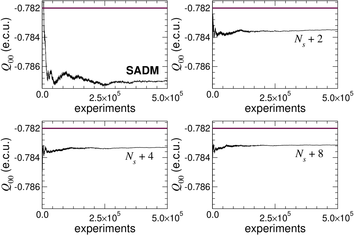
Figure 1: Running average of the point charge, $Q_{00}$, borne by the oxygen atom of water ($N_{s}$ = 2 parameters) as a function of the number of independent realizations, wherein systems of 2 $\times$ 2 (SADM), 4 $\times$ 2, 6 $\times$ 2 and 10 $\times$ 2 linear equations are solved. The thick, dark horizontal line at $Q_{00}$ = $-$0.782 e.c.u. corresponds to the solution of the least-squares problem.

Not too surprisingly, closer examination of the corresponding charge distributions in Figure 2 reveals that as additional grid points are added to the individual realizations, not only does the width of these distributions narrow down, but the latter are progressively reshaped. As was conjectured in [6], the SADM algorithm yields Cauchy distributions, which is apparent from Figure 2. Improvement of the method alters the form of the probability function, now closer to a normal distribution. Interestingly enough, the slightly skewed shape of the distributions, particularly visible on their left-hand side — as a probable manifestation of the incompleteness of the electrostatic model, precludes perfect enveloping by the model distributions, either Cauchy– or Gaussian–like.

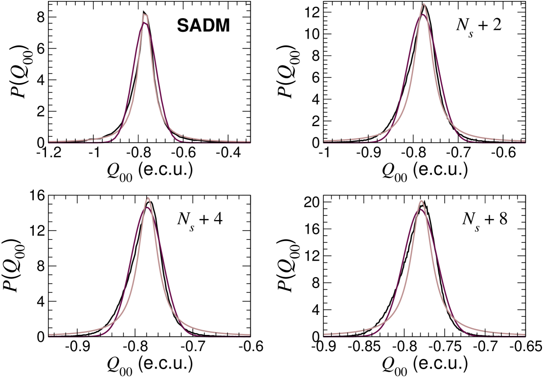
Figure 2: Normalized distributions of the charge, $Q_{00}$, borne by the oxygen atom of water ($N_{s}$ = 2 parameters) obtained from 500,000 independent realizations, wherein systems of 2 $\times$ 2 (SADM), 4 $\times$ 2, 6 $\times$ 2 and 10 $\times$ 2 linear equations are solved (black curves). The light and dark curves correspond, respectively, to numerically fitted Cauchy and Gaussian distributions.

Put together, the present computations reinforce the conclusions drawn hitherto, contradicting in particular the illegitimate assumption that the SADM and the least-squares solutions might coincide [6]. From a numerical standpoint, however, the results obtained from both strategies appear to be reasonably close, thereby warranting that the SADM algorithm should not be obliterated, as it constitutes a valuable pedagogical tool for assessing the appropriateness of electrostatic models.

6 Conclusion

In this work, a probabilistic approach to high-dimensional least-squares approximations has been developed. Originally inspired by the SADM method introduced for the derivation of distributed atomic multipoles from the quantum-mechanical electrostatic potential, this novel approach can be generalized to a wide class of least-squares problems, yielding convergent and efficient numerical schemes in those cases where the space of approximation is very large or where the problem is ill-conditioned.

This novel approach constitutes a marked improvement over the SADM method. Complete analysis of the numerical algorithm in general cases, in terms of both computational effort and optimal error estimation, relies on open and difficult issues prevalent to random matrix problems.

Appendix A Proof of Lemma 3.1

We denote by $\|\cdot\|\left.\vphantom{T_{j_{0}}^{0}}\!\!\right._{F}$ the Schur-Frobenius norm on $n\times m$ matrices

$$\|A\|\left.\vphantom{T_{j_{0}}^{0}}\!\!\right._{F}^{2}=\sum_{i=1}^{m}\sum_{j=1}^{n}a_{ij}^{2}.$$

where $A=(a_{ij})_{1\leq i\leq n,1\leq j\leq m}$. With this notation, we have

$$\|(A^{T}A)^{-1}A^{T}\|\left.\vphantom{T_{j_{0}}^{0}}\!\!\right._{F}^{2}=\mbox{Tr}((A^{T}A)^{-1}A^{T}A(A^{T}A)^{-1})=\mbox{Tr}((A^{T}A)^{-1})\leq\frac{n}{s_{1}(A)}.$$ (A.1)

In addition, for any $v=(v_{1},\ldots,v_{m})\in\mathbb{R}^{m}$, we have

$$\|Av\|\left.\vphantom{T_{j_{0}}^{0}}\!\!\right._{2}^{2} =\sum_{i=1}^{n}\sum_{1\leq j,k\leq m}a_{ij}v_{j}a_{ik}v_{k}$$

$$\leq\frac{1}{2}\Big{(}\sum_{i,j,k}a_{ij}^{2}|v_{j}v_{k}|+\sum_{i,j,k}a_{ik}^{2}|v_{j}v_{k}|\Big{)}$$

$$\leq\|A\|\left.\vphantom{T_{j_{0}}^{0}}\!\!\right._{F}^{2}\|v\|\left.\vphantom{T_{j_{0}}^{0}}\!\!\right._{1}\|v\|\left.\vphantom{T_{j_{0}}^{0}}\!\!\right._{\infty}\leq\|A\|\left.\vphantom{T_{j_{0}}^{0}}\!\!\right._{F}^{2}\|v\|\left.\vphantom{T_{j_{0}}^{0}}\!\!\right._{1}^{2},$$ (A.2)

where we used the inequality $|b_{ij}b_{ik}|\leq\frac{1}{2}(b_{ij}^{2}+b_{ik}^{2})$.

With the notation of Lemma 3.1, using (A.2) and (A.1), we have

$$\|R(X)G(X)\|\left.\vphantom{T_{j_{0}}^{0}}\!\!\right._{2}\leq\sqrt{n}\,s_{1}(\Gamma(X))^{-1/2}\|G(X)\|\left.\vphantom{T_{j_{0}}^{0}}\!\!\right._{1}.$$

Taking the expectation and using Hölder’s inequality, we get

$$\mathbb{E}\|R(X)G(X)\|\left.\vphantom{T_{j_{0}}^{0}}\!\!\right._{2}\leq\sqrt{n}\sqrt{K_{q}(\Gamma)}\Big{(}\mathbb{E}\|G(X)\|\left.\vphantom{T_{j_{0}}^{0}}\!\!\right._{1}^{p}\Big{)}^{1/p}.$$ (A.3)

Now, $Y\mapsto(\mathbb{E}|Y|^{p})^{1/p}$ defines a norm on the set of random vectors on $\Omega$ with finite $p$-th-order moment. We, hence, obtain

$$\big{(}\mathbb{E}\|G(X)\|\left.\vphantom{T_{j_{0}}^{0}}\!\!\right._{1}^{p}\big{)}^{1/p} =\Big{(}\mathbb{E}\Big{(}\sum_{i=1}^{m}|g(X^{(i)})|\Big{)}^{p}\Big{)}^{1/p}$$

$$\leq\sum_{i=1}^{m}\big{(}\mathbb{E}|g(X^{(i)})|^{p}\big{)}^{1/p}=m\|g\|\left.\vphantom{T_{j_{0}}^{0}}\!\!\right._{\mathrm{L}^{p}(\Omega)},$$

and this yields Lemma 3.1 (a).

Lemma 3.1 (b) is obtained from similar computations.

Appendix B Estimates on random matrices

B.1 On the finiteness of $K_{q}(\Gamma)$

As seen in Propositions 3.4 and 3.5, the convergence and the consistency of our algorithm rely on assumptions of the form $K_{q}(\Gamma)<+\infty$, where $K_{q}(\Gamma)$ is given by (3.1). These assumptions correspond to the finiteness of a negative moment of the random variable $s_{1}(\Gamma(X))$. The following proposition provides a condition on the distribution of $s_{1}(\Gamma(X))$ to ensure such integrability properties.

Proposition B.1

Let $Y$ be a random variable satisfying the following estimate: There exist constants $\delta>0$ and $\gamma>0$ such that

$$\forall\epsilon\geq 0,\quad\mathbb{P}(Y\leq\epsilon)\leq(\delta\epsilon)^{\gamma}.$$ (B.1)

Then, for any $0<r<\gamma$,

$$\mathbb{E}(Y^{-r})\leq\frac{\delta^{r}}{1-r/\gamma}.$$ (B.2)

Proof. The proof is based on the following integration by parts, where $\int_{0}^{\infty}h(x)\mathrm{d}\mathbb{P}(Y\in[0,x))$ denotes the Stieltjes integral of the measurable function $h$ with respect to the Stieltjes measure on $[0,\infty)$ associated with the non-decreasing function $x\mapsto\mathbb{P}(Y\in[0,x))$.

$$\mathbb{E}(Y^{-r}) =\int_{0}^{\infty}x^{-r}\mathrm{d}\mathbb{P}(Y\in[0,x))$$

$$=\int_{0}^{\infty}rx^{-r-1}\mathbb{P}(Y\in[0,x))\mathrm{d}x$$

$$\leq r\int_{0}^{\infty}x^{-r-1}((\delta x)^{\gamma}\wedge 1)\mathrm{d}x.$$

If $r<\gamma$,

$$\int_{0}^{\infty}x^{-r-1}((\delta x)^{\gamma}\wedge 1)\mathrm{d}x=\frac{1}{r}\Big{(}\frac{\delta^{r}}{1-r/\gamma}\Big{)},$$

which entails (B.2).  

Of course, the property (B.1) can be strongly problem-dependent. In general situations, this is related to difficult problems on random matrices, which, to our knowledge, have not been solved yet. However, explicit computations are possible in the specific instance where $\Gamma(X)^{T}\Gamma(X)$ has the Wishart distribution (see Subsections 3.5 and below).

In the case where the matrix $\Gamma^{T}(X)\Gamma(X)$ is not a.s. invertible, the method described in Section 4 consists in taking expectations conditionally to $\{s_{1}(\Gamma(X))>\sigma\}$ for some $\sigma>0$. A quantitative analysis of our method relies on estimates on $K_{q}^{\sigma}(\Gamma)$ defined in (4.2) (see Propositions 4.1 and 4.2). The following result generalizes Proposition B.1 to the case where $\sigma>0$. Its proof is very similar to that of Proposition B.1. We will, hence, omit it here.

Proposition B.2

Fix $\sigma\geq 0$ and assume that random variable $Y$ satisfies the following estimate: There exist constants $\delta$ and $\gamma$ such that

$$\forall\,\epsilon\geq\sigma,\quad\mathbb{P}(Y\leq\epsilon)\leq(\delta\epsilon)^{\gamma}.$$ (B.3)

Then, for any $r\not=\gamma$, if $0<\sigma<\delta^{-1}$,

$$\mathbb{E}(Y^{-r}\mid Y\geq\sigma)\leq\frac{\delta^{r}}{1-(\delta\sigma)^{\gamma}}\Big{(}\frac{1}{1-r/\gamma}+\frac{(\delta\sigma)^{-(r-\gamma)}}{1-\gamma/r}\Big{)}.$$ (B.4)

This result is used to obtained explicit estimates on our algorithm in the case where the matrix $\Gamma(X)$ has sub-Gaussian entries (see Sections 4.2 and B.3).

B.2 Explicit estimates in the Wishart case

The goal of this section is to prove the following result.

Proposition B.3

In the Wishart case (see Section 3.5), assume that $f\in\mathrm{L}^{p}(\Omega)$ and $\rho(\bar{\beta})\in\mathrm{L}^{p}(\Omega)$ with $p>2$. Then, the convergence of the algorithm (in the sense that $\textup{Tr}(\textup{Cov}(\beta))<+\infty$, see Proposition 3.4) holds if

$$m>n+\frac{p+2}{p-2}.$$

In the case where $\rho(\bar{\beta})\in\mathrm{L}^{\infty}(\Omega)$, this condition corresponds to $m\geq n+2$ and the computational cost of the algorithm is bounded by

$$C\varepsilon^{-2}\,\frac{n^{3}m^{4}\log n}{(m-n+1)(m-n-1)}\|\rho(\bar{\beta})\|\left.\vphantom{T_{j_{0}}^{0}}\!\!\right._{\mathrm{L}^{\infty}}^{2},$$

where $\varepsilon$ is the required precision and the constant $C$ is independent of $n$ and $m$. The optimal value $m^{*}$ of $m$ in the previous bound satisfies

$$m^{*}\sim 2n$$

when $n\rightarrow+\infty$, and the corresponding computational cost is bounded by

$$C^{\prime}\varepsilon^{-2}n^{5}\log n\|\rho(\bar{\beta})\|\left.\vphantom{T_{j_{0}}^{0}}\!\!\right._{\mathrm{L}^{\infty}}^{2}.$$

In addition, the consistency error of Proposition 3.5 is bounded by

$$C^{\prime\prime}n\|\rho(a)\|\left.\vphantom{T_{j_{0}}^{0}}\!\!\right._{\mathrm{L}^{\infty}}.$$

Our computations are based on the following estimate on the law of the smallest eigenvalue of Wishart matrices [5, Lemma 3.3], which reads with our notation as follows. For all $m\geq n\geq 2$, let

$$k=m-n+1.$$

The density $p(x)$ of $s_{1}(\Gamma(X))$ then satisfies

$$L_{n,m}e^{-nx/2}x^{\frac{k}{2}-1}\leq p(x)\leq L_{n,m}e^{-x/2}x^{\frac{k}{2}-1},\quad\forall x>0,$$ (B.5)

where

$$L_{n,m}=\frac{2^{\frac{k}{2}-1}\Phi(\frac{m+1}{2})}{\Phi(\frac{n}{2})\Phi(k)},$$ (B.6)

where $\Phi$ is the Gamma function, defined for all $x>0$ by

$$\Phi(x)=\int_{0}^{+\infty}e^{-t}t^{x-1}\mathrm{d}t.$$

Lemma B.4

For all $m\geq n\geq 2$, the random variable $Y=s_{1}(\Gamma(X))$ satisfies (B.1) for

$$\gamma=\frac{m-n+1}{2}=\frac{k}{2}$$

$$\mbox{and}\quad\delta=e^{2}\frac{m}{k^{2}}.$$

Moreover, the constant $\gamma$ above is the smallest such that (B.1) holds for all $\varepsilon>0$ for some constant $\delta$.

Proof. This result is based on the following bounds for the Gamma function [5, Lemma 2.7]. For all $x>0$,

$$\sqrt{2\pi}\>x^{x+\frac{1}{2}}e^{-x}<\Phi(x+1)=x\Phi(x)<\sqrt{2\pi}\>x^{x+\frac{1}{2}}e^{-x+\frac{1}{12x}}.$$

These inequalities can be plugged into (B.6) to get that, for all $\varepsilon>0$,

$$\mathbb{P}(s_{1}(\Gamma(X))\leq\varepsilon) \leq\frac{n\>2^{\gamma-1}\Phi(\frac{m-1}{2}+1)}{\Phi(\frac{n}{2}+1)2\gamma\Phi(2\gamma)}\>\gamma\int_{0}^{\varepsilon}x^{\gamma-1}\mathrm{d}x$$

$$\leq\frac{\frac{n}{2}2^{\gamma}\sqrt{2\pi}(\frac{m-1}{2})^{\frac{m}{2}}e^{-\frac{m-1}{2}+\frac{1}{6(m-1)}}}{\sqrt{2\pi}(\frac{n}{2})^{\frac{n+1}{2}}e^{-\frac{n}{2}}\sqrt{2\pi}(2\gamma)^{2\gamma+\frac{1}{2}}e^{-2\gamma}}\>\varepsilon^{\gamma}$$

$$\leq\frac{e^{1+\frac{1}{6(m-1)}}}{2\sqrt{\pi\gamma}}\>\frac{(\frac{m-1}{2})^{\frac{m}{2}}}{(\frac{n}{2})^{\frac{n-1}{2}}}\>\Big{(}\frac{2e^{2}\varepsilon}{4\gamma^{2}e}\Big{)}^{\gamma}.$$

Now,

$$\frac{(\frac{m-1}{2})^{\frac{m}{2}}}{(\frac{n}{2})^{\frac{n-1}{2}}}=\Big{(}\frac{m-1}{n}\Big{)}^{\frac{n-1}{2}}\Big{(}\frac{m-1}{2}\Big{)}^{\gamma} \leq\Big{(}1+\frac{k-2}{n}\Big{)}^{\frac{n}{2}}\Big{(}\frac{m-1}{2}\Big{)}^{\gamma}$$

$$\leq e^{\frac{k-2}{2}}\Big{(}\frac{m-1}{2}\Big{)}^{\gamma}=\frac{1}{e}\Big{(}\frac{e(m-1)}{2}\Big{)}^{\gamma}.$$

Combining this inequality with the facts that $m-1\geq 1$ and $\gamma\geq 1/2$ yields

$$\mathbb{P}(s_{1}(\Gamma(X))\leq\varepsilon)\leq\frac{e^{1/6}}{\sqrt{2\pi}}\Big{(}\frac{e^{2}(m-1)}{4\gamma^{2}}\>\varepsilon\Big{)}^{\gamma}\leq\Big{(}\frac{e^{2}m}{k^{2}}\>\varepsilon\Big{)}^{\gamma}.$$

Because of (B.5), we have that $p(x)\sim L_{n,m}x^{\gamma-1}$ as $x\rightarrow 0$. Therefore, one easily sees that $\gamma=k/2$ is the minimal value of $\gamma$ for (B.1) to holds.  

Using this result and Proposition B.1, we immediately obtain the following:

Proposition B.5

Let $m>n$ be given and assume that the random matrix $\Gamma(X)^{T}\Gamma(X)$ associated with the function $\Gamma$ defined in (2.7) follows a Wishart distribution. Let $q$ be such that

$$1\leq q<k=m-n+1.$$ (B.7)

Then we have

$$K_{q}(\Gamma)\leq\frac{e^{2}m}{k^{2}}\Big{(}1-\frac{q}{k}\Big{)}^{-\frac{2}{q}}$$ (B.8)

where $K_{q}$ is defined in (3.1).

Combining this result and the result of Proposition 3.4, if $\rho(\bar{\beta})\in\mathrm{L}^{p}(\Omega)$ with $p>2$ , the convergence of the algorithm is ensured if $K_{q}<\infty$ in (3.8) with $2p^{-1}+2q^{-1}=1$. This means, (see (B.7))

$$2\leq\frac{2p}{p-2}<m-n+1$$

or equivalently

$$m>n+\frac{p+2}{p-2}.$$

Assume still that $\rho(\bar{\beta})\in\mathrm{L}^{\infty}(\Omega)$. Using (B.8) with $q=2$, it can be seen in view of (3.12) that the cost of the algorithm is bounded by

$$C\varepsilon^{-2}n^{3}m^{3}\log n\,\frac{m}{k^{2}}\Big{(}1-\frac{2}{k}\Big{)}^{-1}\|\rho(\bar{\beta})\|\left.\vphantom{T_{j_{0}}^{0}}\!\!\right._{\mathrm{L}^{\infty}}^{2}.$$

for some constant $C$ independent of $n$ and $m$. Using the notation $\gamma=k/2$, we can rewrite this cost in term of $\gamma$ as

$$C^{\prime}\varepsilon^{-2}n^{3}\log n\,\frac{(n+2\gamma-1)^{4}}{\gamma^{(}\gamma-1)}\|\rho(\bar{\beta})\|\left.\vphantom{T_{j_{0}}^{0}}\!\!\right._{\mathrm{L}^{\infty}}^{2}.$$

To determine the optimal choice of $m$, let us now try to find the optimal number $\gamma$ that minimizes this cost. The derivative of this expression with respect to $\gamma$ has the same sign as

$$8\gamma(\gamma-1)-(n+2\gamma-1)(2\gamma-1)=4\gamma^{2}-2(n+2)\gamma+n-1.$$

Since this quantity is negative if $\gamma=1/2$, the only root of this polynomial greater than $1$ is given by

$$\gamma^{*}=\frac{n+2+\sqrt{n^{2}+8}}{4},$$

which is the optimal choice of $\gamma$ in terms of computational effort. This yields an optimal choice $m^{*}\sim 2\gamma^{*}+n-1$. Note that for large $n$, we have $\gamma^{*}\sim n/2$ and $m^{*}\sim 2n$.

With this optimal choice, the computational cost of the algorithm can be written as

$$C_{n}\varepsilon^{-2}\,\|\rho(\bar{\beta})\|\left.\vphantom{T_{j_{0}}^{0}}\!\!\right._{\mathrm{L}^{\infty}}^{2}\quad\mbox{with}\quad C_{n}\sim Cn^{5}\log n\quad\mbox{as}\quad n\to+\infty.$$

Considering a similar calculation with $q=1$, we can easily see that the consistency error of Proposition 3.2 for this choice of parameters can be bounded by

$$C^{\prime}_{n}\|\rho(a)\|\left.\vphantom{T_{j_{0}}^{0}}\!\!\right._{\mathrm{L}^{\infty}}\quad\mbox{with}\quad C^{\prime}_{n}\sim C^{\prime}n\quad\mbox{as}\quad n\to+\infty.$$

B.3 Explicit estimates in the sub-Gaussian case

The goal of this section is to prove the following result.

Proposition B.6

In the sub-Gaussian case (see Section 4.2), assume that $f\in\mathrm{L}^{\infty}(\Omega)$ and $\rho(\bar{\beta})\in\mathrm{L}^{\infty}(\Omega)$. Then, there exists explicit constants $A$ and $B$ such that, if

$$\sigma=\frac{B^{2}m^{2}(\sqrt{m}-\sqrt{n-1})^{2}}{A(m-n+1)^{2}}e^{-2Bm/(m-n+1)},$$

the computational cost of our algorithm is bounded by

$$C\varepsilon^{-2}\,\frac{n^{3}m^{4}\log n}{(m-n+1)(m-n-1)}\|\rho(\bar{\beta})\|\left.\vphantom{T_{j_{0}}^{0}}\!\!\right._{\mathrm{L}^{\infty}}^{2},$$ (B.9)

where $\varepsilon$ is the required precision and the constant $C$ is independent of $n$ and $m$. Again, the optimal value $m^{*}$ of $m$ in the previous bound satisfies $m^{*}\sim 2n$ as $n\rightarrow+\infty$.
For such a choice of $m$, we obtain

$$\sigma\sim C^{\prime}\,n$$ (B.10)

for an explicit constant $C^{\prime}$.

With our notations, Theorem 1.1 of [20] writes as follows: there exist explicit constants $A$ and $B$ depending only on $R$ such that, for all $m\geq n$ and all $\epsilon>0$,

$$\mathbb{P}\Big{(}s_{1}(\Gamma(X))\leq\epsilon(\sqrt{m}-\sqrt{n-1})^{2}\Big{)}\leq(A\epsilon)^{(m-n+1)/2}+e^{-Bm}.$$ (B.11)

Writing just like in Subsection B.2 $k$ for $m-n+1$, it can be seen that

$$\begin{array}[]{rcl}\mathbb{P}(s_{1}(\Gamma(X))\leq\varepsilon)&\leq&\displaystyle\Big{(}\frac{\sqrt{A\varepsilon}}{\sqrt{m}-\sqrt{n-1}}\Big{)}^{k}+\big{(}e^{-Bm/k}\big{)}^{k}\\[8.61108pt] &\leq&\displaystyle\Big{(}\frac{\sqrt{A\varepsilon}}{\sqrt{m}-\sqrt{n-1}}+e^{-Bm/k}\Big{)}^{k}.\end{array}$$

Eq. (B.3), therefore, holds for $Y=s_{1}(\Gamma(X))$ and

$$\sigma\geq\sigma_{0}:=\frac{B^{2}m^{2}(\sqrt{m}-\sqrt{n-1})^{2}}{k^{2}A}e^{-2Bm/k},$$

$$\delta=\frac{(1+k/Bm)^{2}A}{(\sqrt{m}-\sqrt{n-1})^{2}}$$

$$\mbox{and}\quad\gamma=\frac{k}{2}.$$

Note that, since $\delta\sigma_{0}=(1+Bm/k)^{2}e^{-2Bm/k}<1$, the inequality in (B.3) is not trivial and supplies some information on the law of $s_{1}(\Gamma(X))$.

As in Subsection B.2, the inequality (B.4) can be combined with the results of Propositions 4.2 and 4.1 to obtain a precise error estimate and convergence bounds in this case.

Such computations are, however, cumbersome because the optimal choice of $\sigma$ cannot be determined explicitly. Taking $\sigma=\sigma_{0}$ as in Proposition B.6 and under the assumption that $\rho(\bar{\beta}^{\sigma})\in\mathrm{L}^{\infty}(\Omega)$, because of Proposition B.2, the computational cost is smaller than

$$C\varepsilon^{-2}n^{3}\log n\|\rho(\bar{\beta}^{\sigma})\|\left.\vphantom{T_{j_{0}}^{0}}\!\!\right._{\mathrm{L}^{\infty}}^{2}\frac{m^{3}\delta}{(1-(\delta\sigma)^{\gamma})^{2}}\Big{(}\frac{1}{1-1/\gamma}+\frac{(\delta\sigma)^{\gamma-1}}{1-\gamma}\Big{)}$$

If one assumes that $(\sigma_{0}\delta)^{\gamma}\rightarrow 0$ as $n\rightarrow+\infty$, observing that

$$\delta=\frac{(\sqrt{m}+\sqrt{n-1})^{2}(1+k/Bm)^{2}A}{k^{2}}\leq\frac{Cm}{k^{2}},$$

the cost is bounded from above by

$$C\varepsilon^{-2}n^{3}\log n\frac{m^{4}}{\gamma(\gamma-1)}\|\rho(\bar{\beta}^{\sigma})\|\left.\vphantom{T_{j_{0}}^{0}}\!\!\right._{\mathrm{L}^{\infty}}^{2}$$

for $\gamma>1$. We recognize the same cost as in Subsection 3.5. The optimal choice of $\gamma$, therefore, behaves as $n/2$ as $n\rightarrow+\infty$ — and for this choice we indeed have $(\sigma_{0}\delta)^{\gamma}\rightarrow 0$, which validates the previous computation. Therefore, for this choice of parameters, the cost is bounded by

$$C\varepsilon^{-2}n^{5}\log n\|\rho(\bar{\beta}^{\sigma})\|\left.\vphantom{T_{j_{0}}^{0}}\!\!\right._{\mathrm{L}^{\infty}}^{2}$$

for some constant $C>0$.

One can check that any other choice of $\sigma$ yields the same order in $n$ as $n\rightarrow+\infty$, should one choose $\gamma\sim n/2$.

It ought to be noted that these bounds do not allow one to pick $\sigma=0$. As far as we know, this seems to be an open and difficult question to prove that (B.11) holds without the right-hand-side, additive term $e^{-Bm}$. In particular, it requires additional assumptions to hold — e.g. random variable $h(Y)$, where $Y$ has law $\nu$, has no atom, i.e. that $\nu(\{h=y\})=0$ for all $y\in\mathbb{R}$ (otherwise, the matrix $\Gamma(X)$ could have $m-n$ identical rows, and, thus, have a rank less than $n$, with non-zero probability).

References

- [1] T. W. Anderson. An introduction to multivariate statistical analysis. Wiley Series in Probability and Mathematical Statistics: Probability and Mathematical Statistics. John Wiley & Sons Inc., New York, second edition, 1984.
- [2] J. G. Ángyán, C. Chipot, F. Dehez, C. Hättig, G. Jansen, and C. Millot. Opep: A tool for the optimal partitioning of electric properties. J. Comput. Chem., 24:997–1008, 2003.
- [3] C. I. Bayly, P. Cieplak, W. D. Cornell, and P. A. Kollman. A well–behaved electrostatic potential based method using charge restraints for deriving atomic charges: The resp model. J. Phys. Chem., 97:10269–10280, 1993.
- [4] A. Bjorck. Numerical Methods for Least Squares Problems. SIAM, Philadelphia, PA, 1996.
- [5] Zizhong Chen and Jack J. Dongarra. Condition numbers of Gaussian random matrices. SIAM J. Matrix Anal. Appl., 27(3):603–620 (electronic), 2005.
- [6] C. Chipot, J. G. Ángyán, and C. Millot. Statistical analysis of distributed multipoles derived from the molecular electrostatic potential. Mol. Phys., 94:881–895, 1998.
- [7] L. E. Chirlian and M. M. Francl. Atomic charges derived from electrostatic potentials: A detailed study. J. Comput. Chem., 8:894–905, 1987.
- [8] W. D. Cornell and C. Chipot. Alternative approaches to charge distribution calculations. In P. v. R. Schleyer, N. L. Allinger, T. Clark, J. Gasteiger, P. A. Kollman, H. F. Schaefer III, and P. R. Schreiner, editors, Encyclopedia of computational chemistry, volume 1, pages 258–263. Wiley and Sons, Chichester, 1998.
- [9] W. D. Cornell, P. Cieplak, C. I. Bayly, I. R. Gould, K. M. Merz Jr., D. M. Ferguson, D. C. Spellmeyer, T. Fox, J. C. Caldwell, and P. A. Kollman. A second generation force field for the simulation of proteins, nucleic acids, and organic molecules. J. Am. Chem. Soc., 117:5179–5197, 1995.
- [10] S. R. Cox and D. E. Williams. Representation of the molecular electrostatic potential by a net atomic charge model. J. Comput. Chem., 2:304–323, 1981.
- [11] Alan Edelman. Eigenvalues and condition numbers of random matrices. SIAM J. Matrix Anal. Appl., 9(4):543–560, 1988.
- [12] Alan Edelman. The distribution and moments of the smallest eigenvalue of a random matrix of Wishart type. Linear Algebra Appl., 159:55–80, 1991.
- [13] M. M. Francl, C. Carey, L. E. Chirlian, and D. M. Gange. Charges fit to the electrostatic potentials. ii. can atomic charges be unambiguously fit to electrostatic potentials ? J. Comput. Chem., 17:367–383, 1996.
- [14] M. J. Frisch, G. W. Trucks, H. B. Schlegel, G. E. Scuseria, M. A. Robb, J. R. Cheeseman, J. A. Montgomery, Jr., T. Vreven, K. N. Kudin, J. C. Burant, J. M. Millam, S. S. Iyengar, J. Tomasi, V. Barone, B. Mennucci, M. Cossi, G. Scalmani, N. Rega, G. A. Petersson, H. Nakatsuji, M. Hada, M. Ehara, K. Toyota, R. Fukuda, J. Hasegawa, M. Ishida, T. Nakajima, Y. Honda, O. Kitao, H. Nakai, M. Klene, X. Li, J. E. Knox, H. P. Hratchian, J. B. Cross, C. Adamo, J. Jaramillo, R. Gomperts, R. E. Stratmann, O. Yazyev, A. J. Austin, R. Cammi, C. Pomelli, J. W. Ochterski, P. Y. Ayala, K. Morokuma, G. A. Voth, P. Salvador, J. J. Dannenberg, V. G. Zakrzewski, S. Dapprich, A. D. Daniels, M. C. Strain, O. Farkas, D. K. Malick, A. D. Rabuck, K. Raghavachari, J. B. Foresman, J. V. Ortiz, Q. Cui, A. G. Baboul, S. Clifford, J. Cioslowski, B. B. Stefanov, G. Liu, A. Liashenko, P. Piskorz, I. Komaromi, R. L. Martin, D. J. Fox, T. Keith, M. A. Al-Laham, C. Y. Peng, A. Nanayakkara, M. Challacombe, P. M. W. Gill, B. Johnson, W. Chen, M. W. Wong, C. Gonzalez, and J. A. Pople. Gaussian 03 Revision C.02. Gaussian Inc., Wallingford, CT, 2004.
- [15] E. J. Heller. Time dependent approach to semiclassical dynamics. J. Chem. Phys., 62:1544–1555, 1975.
- [16] A. D. MacKerell Jr., D. Bashford, M. Bellott, R. L. Dunbrack Jr., J. D. Evanseck, M. J. Field, S. Fischer, J. Gao, H. Guo, S. Ha, D. Joseph-McCarthy, L. Kuchnir, K. Kuczera, F. T. K. Lau, C. Mattos, S. Michnick, T. Ngo, D. T. Nguyen, B. Prodhom, W. E. Reiher III, B. Roux, M. Schlenkrich, J. C. Smith, R. Stote, J. Straub, M. Watanabe, J. Wiórkiewicz-Kuczera, D. Yin, and M. Karplus. All–atom empirical potential for molecular modeling and dynamics studies of proteins. J. Phys. Chem. B, 102:3586–3616, 1998.
- [17] S. Maire and C. De Luigi. Quasi-monte carlo quadratures for multivariate smooth functions. Applied Numerical Mathematics, 56:146–162, 2006.
- [18] Yves Meyer and Hong Xu. Wavelet analysis and chirps. Appl. Comput. Harmon. Anal., 4(4):366–379, 1997.
- [19] V. V. Petrov. Sums of independent random variables. Springer-Verlag, New York, 1975. Translated from the Russian by A. A. Brown, Ergebnisse der Mathematik und ihrer Grenzgebiete, Band 82.
- [20] M. Rudelson and R. Vershynin. The smallest singular value of a random rectangular matrix. Comm. Pure Appl. Math., 62(12):1707–1739, 2009.