Proposal for a cumulant-based Bell test for mesoscopic junctions

Abstract

The creation and detection of entanglement in solid state electronics is of fundamental importance for quantum information processing. We prove that second-order quantum correlations can be always interpreted classically and propose a general test of entanglement based on the violation of a classically derived inequality for continuous variables by fourth-order quantum correlation functions. Our scheme provides a way to prove the existence of entanglement in a mesoscopic transport setup by measuring higher order cumulants without requiring the additional assumption of a single charge detection.

I Introduction

The quantum theory cannot be explained by any underlying classical local hidden variable model, according to the Bell theorem.bel It allows to verify that, contrary to the classical case, the results of quantum mechanics violate a special inequality bein under the conditions: (i) dichotomy of measurement outcomes or their restricted set in some generalizations, cglmp (ii) freedom of choice of the measured observables will and (iii) the time of the choice and measurement of the observable shorter than the communication time between the observers. Relaxing any of the above three conditions opens a (i) detection, (ii) free will or (iii) communication loophole, which permits to construct a local hidden variable model explaining the results of the experiments.loop The performed experimental tests confirmed the violation of Bell inequality with all the loopholes closed belx but never all simultaneously. loopfree The remaining loophole is ”closed” by a reasonable additional assumption. The Bell test is also stronger than the entanglement criterion, viz. the nonseparability of states, ent which assumes a finite dimension of the Hilbert space. Loophole-free violation of Bell inequality, not just entanglement, is also necessary for successful quantum cryptography,gis06 although the loopholes are probably less important than decoherence problems. scalrev

There is a growing interest in tests of nonclassicality in solid state systems, especially electrons in noninteracting mesoscopic junctions.entsol ; entrev ; heiblum Unlike bosons, even noninteracting fermions in the Fermi sea can get entangled due to the Pauli exclusion principle. For example, entangled electron-hole pairs are created at both sides of a biased tunnel junction. So far the efforts concentrated on testing entanglement by second-order current correlations.excoop Unfortunately, to make the genuine Bell test, the charge flow quantization must be measured directly, which has so far only been achieved in quantum dots.dot However, in tunnel junctions and quantum point contacts rather current cumulants fcs are directly accessible and, so far, the noise noi and the third cumulant three of the current have been measured. The quantization of charge flow is also not so evident at short timescales or high frequencies when vacuum fluctuations of the Fermi sea play a role. vac In some cases, energy filters can restore the Bell correlations at short times,han at the expense of opening the detection loophole (most of electrons get lost).fazio

In this paper we present a genuine Bell test for mesoscopic junctions, which does not require the usual assumption that only quantized charge transfers are detected. Instead of quantized events, we shall treat the current as a continuous, time-dependent observable. As we will show-second order correlations in this case can be always explained classically. Hence, we need a Bell inequality for unbounded variables, without a sharp dichotomy, which will require to exploit correlation functions and higher moments/cumulants. Such an inequality has been recently discovered belcon but the violation requires at least 10 observers and 20th-order averages. Moreover, the corresponding Bell-like state is not feasible in mesoscopic junctions. Our inequality will need only two observers and maximally fourth moments/cumulants. The inequality reduces to the usual Bell inequality if the quantization is granted. A violation is possible in a mesoscopic tunnel junction with spin filtered leads or pierced by tunable magnetic flux.

We first prove weak positivity (classicality of second order quantum correlations), next conctruct the Bell-type inequality based of fourth order moments, then implement it in the tunnel junction and finally discuss possible loopholes.

II Weak positivity

Let us begin with the simple proof that first- and second order correlations functions can be always reproduced classically. To see this, consider a real symmetric correlation matrix $2C_{ij}=2\langle A_{i}A_{j}\rangle=\mathrm{Tr}\hat{\rho}\{\hat{A}_{i},\hat{A}_{j}\}$ with $\{\hat{A},\hat{B}\}=\hat{A}\hat{B}+\hat{B}\hat{A}$ for arbitrary, even noncommuting observables $\hat{A}_{i}$ and the density matrix $\hat{\rho}$. This includes all possible first-order averages $\langle A_{i}\rangle$ by setting one observable to identity or subtracting averages ($A_{i}\to A_{i}-\langle A_{i}\rangle$). Since $\mathrm{Tr}\hat{\rho}\hat{X}^{2}\geq 0$ for $\hat{X}=\sum_{i}\lambda_{i}\hat{A}_{i}$ with arbitrary real $\lambda_{i}$, we find that the correlation matrix $C$ is positive definite and any correlation can be simulated by a classical Gaussian distribution $\rho\propto\exp(-\sum_{ij}{C^{-1}}_{ij}A_{i}A_{j}/2)$. Note that the often used dichotomy $A=\pm 1$ is equivalent to $\langle(A^{2}-1)^{2}\rangle=0$, which requires $\langle A^{4}\rangle$. Moreover, every classical inequality $\langle(f(\{A_{i}\})^{2}\rangle\geq 0$ contains the highest correlator of even order. Hence, to detect nonclassical effects with unbounded observables, we have to consider the fourth moments.

III Bell-type inequality

As usual we introduce two separate observers, Alice and Bob that are free to choose between two observables, ($A$, $A^{\prime}$) and ($B$, $B^{\prime}$), respectively. The measurements can give arbitrary outcomes (not just $\pm 1$). We have the following algebraic identities:

$$(AB+A^{\prime}B+AB^{\prime}-A^{\prime}B^{\prime})(A^{2}+A^{\prime 2}+B^{2}+B^{\prime 2})$$

$$=2(A^{3}B+AB^{3}+A^{\prime 3}B+A^{\prime}B^{3}$$

$$+A^{3}B^{\prime}+AB^{\prime 3}-A^{\prime 3}B^{\prime}-A^{\prime}B^{\prime 3})$$ (1)

$$+AB[(A^{\prime 2}-B^{2})+(B^{\prime 2}-A^{2})]$$

$$+A^{\prime}B[(A^{2}-B^{2})+(B^{\prime 2}-A^{\prime 2})]$$

$$+AB^{\prime}[(A^{\prime 2}-B^{\prime 2})+(B^{2}-A^{2})]$$

$$-A^{\prime}B^{\prime}[(A^{2}-B^{\prime 2})+(B^{2}-A^{\prime 2})]$$

and

$$(AB+A^{\prime}B+AB^{\prime}-A^{\prime}B^{\prime})^{2}=(A^{2}+A^{\prime 2})(B^{2}+B^{\prime 2})$$

$$+AA^{\prime}[(B^{2}-A^{2})+(B^{2}-A^{\prime 2})]$$

$$-AA^{\prime}[(B^{\prime 2}-A^{2})+(B^{\prime 2}-A^{\prime 2})]$$

$$+BB^{\prime}[(A^{2}-B^{2})+(A^{2}-B^{\prime 2})]$$

$$-BB^{\prime}[(A^{\prime 2}-B^{2})+(A^{\prime 2}-B^{\prime 2})].$$ (2)

We now apply the Cauchy inequality $2|\langle xy\rangle|\leq\langle x^{2}+y^{2}\rangle$ to $x=AB+A^{\prime}B+AB^{\prime}-A^{\prime}B^{\prime}$, $y=(A^{2}+A^{\prime 2}+B^{2}+B^{\prime 2})/2$, then $|\langle X\rangle|\leq|\langle X+Y\rangle|+|\langle Y\rangle|$ for $X+Y$ given by the right-hand side of (1) and $X=2(A^{3}B+AB^{3}+A^{\prime 3}B+A^{\prime}B^{3}+A^{3}B^{\prime}+AB^{\prime 3}-A^{\prime 3}B^{\prime}-A^{\prime}B^{\prime 3})$. Then we use again the Cauchy inequality for $x,y=A^{2},A^{\prime 2},B^{2},B^{\prime 2}$. On the right-hand sides of (1) and (2) we have 16 terms of the form $\pm\langle AA^{\prime}(B^{2}-A^{\prime 2})\rangle$. To decouple those containing simultaneous measurements of $A(B)$ and $A^{\prime}(B^{\prime})$ we first use the triangle inequality $|\langle\sum_{i}x_{i}\rangle|\leq\sum_{i}|\langle x_{i}\rangle|$ for the sum of all terms and finally the Cauchy-Bunyakovsky-Schwarz-type inequality $|\langle AA^{\prime}(A^{2}-B^{2})\rangle|\leq\langle A^{4}\rangle^{1/4}\langle A^{\prime 4}\rangle^{1/4}\langle(A^{2}-B^{2})^{2}\rangle^{1/2}$ to each term individually. We end up with our main inequality

$$|\langle AB(A^{2}+B^{2})\rangle+\langle A^{\prime}B(A^{\prime 2}+B^{2})\rangle$$

$$+\langle AB^{\prime}(A^{2}+B^{\prime 2})\rangle-\langle A^{\prime}B^{\prime}(A^{\prime 2}+B^{\prime 2})\rangle|/2\leq$$ (3)

$$\left(\langle A^{4}\rangle+\langle A^{\prime 4}\rangle+\langle B^{4}\rangle+\langle B^{\prime 4}\rangle\right)/2+$$

$$\frac{1}{4}\sum_{C,D,E=\{A,A^{\prime},B,B^{\prime}\}}^{D\neq C;E\neq C,D,D^{\prime}}\sqrt{\sqrt{\left\langle C^{4}\right\rangle}\sqrt{\langle D^{4}\rangle}\left\langle\left(D^{2}-E^{2}\right)^{2}\right\rangle},$$

where $D^{\prime}=A(B)$ when $D=A^{\prime}(B^{\prime})$. For the complete derivation, see the Appendix.

The inequality contains up to fourth-order averages which is a trade-off for relaxing the condition of dichotomy (or trichotomy, considering also $0$). It reduces to the standard Bell inequality

$$|\langle AB\rangle+\langle A^{\prime}B\rangle+\langle AB^{\prime}\rangle-\langle A^{\prime}B^{\prime}\rangle|\leq 2$$ (4)

if we restrict the possible values of $A$,$A^{\prime}$,$B$,$B^{\prime}$ to $\pm 1$. If all observables are allowed to take the additional value $0$ only simultaneously then the inequality still reproduces Bell multiplied by the probability of nonzero outcomes. All correlations in the inequality are measurable also in a Bell-type test, because none of them contains $AA^{\prime}$ or $BB^{\prime}$. Hence, we can say that the degrees of freedom measured by $A^{(\prime)}$ and $B^{(\prime)}$ are entangled if the inequality (3) of their correlators is violated. We emphasize that this requires only the assumption of nonnegative probability distribution $\rho(A,A^{\prime},B,B^{\prime})\geq 0$ and provides an unambiguous proof for entanglement.

Returning to quantum mechanics, let us take the standard Bell state bein $\hat{\rho}=(\hat{1}-\hat{\boldsymbol{\sigma}}_{A}\cdot\hat{\boldsymbol{\sigma}}_{B})/4$, $\boldsymbol{\sigma}=(\sigma_{1},\sigma_{2},\sigma_{3})$, with $\hat{\sigma}_{i}$ – standard spin Pauli matrices $\{\hat{\sigma}_{i},\hat{\sigma}_{j}\}=2\delta_{ij}\hat{1}$ acting in Hilbert space $\mathcal{H}_{A}\otimes\mathcal{H}_{B}$, $\hat{A}^{(\prime)}=\boldsymbol{a}^{(\prime)}\cdot\hat{\boldsymbol{\sigma}}_{A}$, $|\boldsymbol{a}^{(\prime)}|=1$ ($A\leftrightarrow B$) and averages $\langle A^{(\prime)n}B^{(\prime)m}\rangle=\mathrm{Tr}\hat{\rho}\hat{A}^{(\prime)n}\hat{B}^{(\prime)m}$. In particular $\langle A^{(\prime)4}\rangle=\langle B^{(\prime)4}\rangle=\langle A^{(\prime)2}B^{(\prime)2}\rangle=1$ and $\langle A^{(\prime)}B^{(\prime)3}\rangle=\langle A^{(\prime)3}B^{(\prime)}\rangle=-\boldsymbol{a}^{(\prime)}\cdot\boldsymbol{b}^{(\prime)}$. The inequality (3) is violated as it reads $2\sqrt{2}\leq 2$ for $\boldsymbol{a}^{\prime}$,$\boldsymbol{b}$,$\boldsymbol{a}$,$\boldsymbol{b}^{\prime}$ in one plane at angles $0$, $\pi/4$, $\pi/2$, $3\pi/4$, respectively.

IV Test on tunnel junction

Now we implement the Bell example in a beam splitting device involving fermions scattered at a tunnel junction. The junction is described by fermionic operators around the Fermi level.blanter Each operator $\hat{\psi}_{A\bar{n}}$ is denoted by the mode number $n\in\{1..N\}$ and the spin orientation $\sigma$, $\bar{n}=(n,\sigma)$ and $A=L,R$ for left and right going electrons, respectively. Each mode has its own Fermi velocity $v_{n}$ and transmission coefficient $\mathcal{T}_{n}$ (reflection $\mathcal{R}_{n}=1-\mathcal{T}_{n}$). We will assume noninteracting electrons and energy- and spin-independent transmission through the junction. The Hamiltonian is

$$\hat{H}=\sum_{\bar{n}}\int dx\left\{i\hbar v_{n}[\hat{\psi}^{\dagger}_{L\bar{n}}(x)\partial_{x}\hat{\psi}_{L\bar{n}}(x)-L\leftrightarrow R]\right.$$

$$+eV\theta(-x)[\hat{\psi}^{\dagger}_{L\bar{n}}(x)\hat{\psi}_{L\bar{n}}(x)+L\leftrightarrow R]$$

$$\left.+q_{n}\delta(x)[\hat{\psi}^{\dagger}_{L\bar{n}}(x)\hat{\psi}_{R\bar{n}}(-x)+\hat{\psi}^{\dagger}_{R\bar{n}}(x)\hat{\psi}_{L\bar{n}}(-x)]\right\}\,.$$ (5)

The fermionic operators satisfy anticommutation relations $\{\hat{\psi}_{a}(x),\hat{\psi}_{b}(x^{\prime})\}=0$ and $\{\hat{\psi}_{a}(x),\hat{\psi}^{\dagger}_{b}(x^{\prime})\}=\delta_{ab}\delta(x-x^{\prime})$ for $a,b=L\bar{n},R\bar{m}$. The transmission coefficients are $\mathcal{T}_{n}=\cos^{2}(q_{n}/\hbar v_{n})$. The system’s current operator is defined $\hat{I}_{n}(x)=\sum_{\sigma}ev_{n}\hat{\psi}^{\dagger}_{L\bar{n}}(x)\hat{\psi}_{L\bar{n}}(x)-L\leftrightarrow R$ and the density matrix is $\hat{\rho}\propto\exp(-\hat{H}/k_{B}T)$.

The Bell measurement will be performed by adding spin filters or magnetic flux at both sides of the junctions as shown in Fig. 1. In both cases we have to add $\hat{H}^{\prime}=\sum_{ab}\int dx\;eV_{ab}(x)\hat{\psi}^{\dagger}_{a}(x)\hat{\psi}_{b}(x)$ to the Hamiltonian (5) where $V_{ab}(x)$ is scattering potential, localized near detectors. The effect of each part of the Hamiltonian on single-mode wave function can be described by three scattering matrices blanter

$$s_{i}=\left(\begin{array}[]{cc}r_{i}&t_{i}\\ t^{\prime}_{i}&r^{\prime}_{i}\end{array}\right),$$ (6)

where $i=A,T,B$ describe scattering at the left detector, junction and the right detector, respectively. The junction has diagonal transmission and reflection submatrices with $t_{T}=t^{\prime}_{T}=i\sqrt{\mathcal{T}}\hat{1}$. In the case of spin filters we assume $4\times 2$ transmission $2t_{A}=(1+\boldsymbol{a}\cdot\hat{\boldsymbol{\sigma}}\>\>1-\boldsymbol{a}\cdot\hat{\boldsymbol{\sigma}}),$ where $|\boldsymbol{a}|=1$. Alternatively, having a tunable geometry of the scatterer, we could introduce an ”artificial spin” filter taking $\sigma_{1,3}$ acting in the mode space instead of spin space. For magnetic fluxes $r_{A}=0$ and

$$t_{A}=\left(\begin{array}[]{cc}e^{i\phi_{A}}&0\\ 0&1\end{array}\right)\frac{1}{\sqrt{2}}\left(\begin{array}[]{cc}1&1\\ 1&-1\end{array}\right).$$ (7)

where $\phi_{A}$ represents Aharonov-Bohm phase picked on the upper branch. The matrices can be enlarged to represent the $2N$-mode junction.

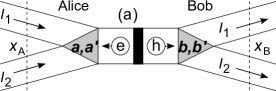
Figure 1: Proposals of experimental setups for the Bell test. In both cases the black bar represents the scattering barrier, producing entangled electron-hole pairs. The tested observable is the difference of currents, $I_{1}-I_{2}$, at left (Alice) or right (Bob) side. The correlations depend on the spin scattering (a) or magnetic fluxes (b).

In both cases, the transmission coefficients for the total scattering matrix are $\mathcal{T}_{11}=\mathcal{T}_{22}=\mathcal{T}(1+\boldsymbol{a}\cdot\boldsymbol{b})/2$ and $\mathcal{T}_{12}=\mathcal{T}_{21}=\mathcal{T}(1-\boldsymbol{a}\cdot\boldsymbol{b})/2$, where $\boldsymbol{a}=(\cos\phi_{A},\sin\phi_{A},0)$ in the case of magnetic fluxes.

As in the previous proposals entsol ; entrev the tunnel barrier produces electron-hole pairs with entangled spins or orbitals. Alice and Bob can test the inequality (3) by measuring the difference between charge fluxes in the upper and lower arm as shown in Fig. 1. For Alice, the measured observable reads in the Heisenberg picture

$$\hat{A}=\int dt\>f(t)(\hat{I}_{1}(x_{A},t)-\hat{I}_{2}(x_{A},t))/e.$$ (8)

for the filter setting $\boldsymbol{a}$. Here $x_{A}$ is the point of measurement, satisfying $\mathrm{max}\{|eV|,k_{B}T\}|x_{A}/v_{n}\hbar|\ll\mathcal{T}$ with $f(t)$ slowly changing on the timescale $\hbar/\mathrm{max}\{|eV|,k_{B}T\}$. One defines analogically $A^{\prime}$ for $\boldsymbol{a}^{\prime}$ and $B$, $B^{\prime}$ for Bob.

The measured probability distribution can be treated as a convolution $\rho(A,B)=\int dA^{\prime}dB^{\prime}\rho_{d}(A-A^{\prime},B-B^{\prime})\varrho(A^{\prime},B^{\prime})$, where $\rho_{d}$ is the Gaussian detection noise (independent of the system and later subtracted) and $\varrho$ is a quasiprobability,our where

$$\langle X_{1}(t_{1})\cdots X_{n}(t_{n})\rangle_{\varrho}=$$ (9)

$$\mathrm{Tr}\hat{\rho}\{\hat{X}_{1}(t_{1}),\{\cdots\{\hat{X}_{n-1}(t_{n-1}),\hat{X}_{n}(t_{n})\}\cdots\}\}/2^{n-1}$$

for time ordered observables, $t_{1}\leq t_{2}\leq\cdots\leq t_{n}$. The detection noise adds $I_{di}$ to the measurement outcome $I_{i}$ with $\langle I_{di}(0)I_{dj}(t)\rangle=e^{2}\delta(t)\delta_{ij}/\tau$. In the interaction-free limit [the sensitivity $\tau$ much smaller than the time resolution of the measurement, the timescale of $f(t)$] one can calculate averages with respect to $\varrho$ using existing methods based on full counting statistics and its extension. entsol ; entrev ; fcs ; blanter ; zaikin1 The averages needed in the inequality (3) can be derived using four-lead full counting statistics generating functionalfcs in the tunneling limit ($\mathcal{T}\ll 1$),

$$S(\chi_{A},\chi_{B})=\ln\langle e^{iA\chi_{A}+iB\chi_{B}}\rangle_{\varrho}$$

$$=N\mathcal{T}\hbar^{-1}\sum_{\alpha,\beta=\pm 1}\sum_{\pm}\int dtf(t)\int dE\times$$ (10)

$$f_{\pm}(E)(1-f_{\mp}(E))(1+\alpha\beta\boldsymbol{a}\cdot\boldsymbol{b})(e^{\pm i\alpha\chi_{A}\pm i\beta\chi_{B}}-1)$$

with Fermi distributions $f_{\pm}(E)=(1+e^{(E\pm eV/2)/k_{B}T})^{-1}$. In our case, one obtains a simple physical picture: the electron-hole Bell pairs are transmitted according to Poissonian statistics. The averages (cumulants and moments) are found by taking derivatives of (10) with respect to $\chi$. In particular, we have $\langle A^{(\prime)}\rangle_{\varrho}=\langle B^{(\prime)}\rangle_{\varrho}=0$ and $\langle A^{(\prime)}B^{(\prime)3}\rangle_{\varrho}=\langle A^{(\prime)3}B^{(\prime)}\rangle_{\varrho}=({\boldsymbol{a}}^{(\prime)}\cdot{\boldsymbol{b}}^{(\prime)})\langle A^{4}\rangle_{\varrho}$, $\langle A^{4}\rangle_{\varrho}=\langle A^{(\prime)4}\rangle_{\varrho}=\langle B^{(\prime)4}\rangle_{\varrho}$ and $\langle A^{2}B^{2}\rangle_{\varrho}=\langle A^{4}\rangle_{\varrho}-2(1-(\boldsymbol{a}\cdot\boldsymbol{b})^{2}))\langle A^{2}\rangle^{2}_{\varrho}$. The inequality (3) gets a simplified form in this particular case,

$$|C(\boldsymbol{a},\boldsymbol{b},\boldsymbol{a}^{\prime},\boldsymbol{b}^{\prime})|\leq 2+2\sum_{\boldsymbol{d}=\boldsymbol{a},\boldsymbol{a}^{\prime}}^{\boldsymbol{e}=\boldsymbol{b},\boldsymbol{b}^{\prime}}\sqrt{(1-(\boldsymbol{d}\cdot\boldsymbol{e})^{2})\langle A^{2}\rangle^{2}_{\varrho}/\langle A^{4}\rangle_{\varrho}},$$ (11)

where $C(\boldsymbol{a},\boldsymbol{b},\boldsymbol{a}^{\prime},\boldsymbol{b}^{\prime})=\boldsymbol{a}\cdot\boldsymbol{b}+\boldsymbol{a}^{\prime}\cdot\boldsymbol{b}+\boldsymbol{a}\cdot\boldsymbol{b}^{\prime}-\boldsymbol{a}^{\prime}\cdot\boldsymbol{b}^{\prime}$. We stress that (11) follows from theoretical predictions and the experimental test still requires the measurement of all averages in (3). We choose $f(t)=\theta_{\delta}(2t_{0}-|t|)$, where $\theta_{\delta}(t)=\theta(t)$ for $|t|\gg\delta$ with a smooth crossover at $|t|\lesssim\delta$.

Having assumed the tunneling limit ($\mathcal{T}\ll 1$), we make the following approximations

$$1/N\mathcal{T}\gg t_{0}\mathrm{max}\{|eV|,k_{B}T\}/h\gg t_{0}/\delta\gg 1$$ (12)

with $2N$ denoting the total number modes going through the barrier. In this limit, all moments and cumulants are equal

$$\langle A^{(\prime)2n}\rangle_{\varrho}\simeq\frac{2eVN\mathcal{T}t_{0}}{h}\coth\left(\frac{eV}{2k_{B}T}\right),\>n>0$$ (13)

Hence the last term on the right-hand side of Eq.  (11) is negligible and the inequality takes the usual form $|C(\boldsymbol{a},\boldsymbol{b},\boldsymbol{a}^{\prime},\boldsymbol{b}^{\prime})|\leq 2$, which can be violated by appropriate choice of the spin axes. Instead of time domain, one can measure correlations in frequency domain (up to $\omega\sim 1/t_{0}$) and make a Fourier transform.han If the scattering is mode-independent then one can assume that the junction consists of minimally $N_{0}\simeq Gh/e^{2}$ independent channels, where $G=2N\mathcal{T}e^{2}/h$ is the total conductance of the junction, and repeat the whole above reasoning with $N$ replaced by $N/N_{0}$ (experimentally – dividing measured cumulants $\langle\langle\cdots\rangle\rangle$ by $N_{0}$).

V Loopholes

The communication loophole is still open, not only because the system is nonrelativistic but also because the measurement time $t_{0}$ is larger than the flight time between detectors ($|x_{A}-x_{B}|/v_{n}$). Let us impose shorter measurement $t_{0}\ll|x_{A}-x_{B}|/v_{n}$. Far from the barrier the vacuum fluctuations of incoming and reflected current do not cancel each other. For the noise measured at frequencies $\omega\gg v_{n}/|x_{A}|$, the incoming and reflected current become independent and the noise saturates to the same value as for the completely open barrier,

$$\int dt\>e^{i\omega t}\mathrm{Tr}\{\hat{I}_{i}(t),\hat{I}_{j}(0)\}\hat{\rho}/2=\frac{N\delta_{ij}\omega}{2\pi}\coth\left(\frac{\hbar\omega}{2k_{B}T}\right).$$ (14)

Hence for $t_{0}\ll|x_{A}|/v_{n}$, we have

$$\langle A^{2}\rangle_{\varrho}\simeq 2N\pi^{-2}\ln\left[\frac{\sinh(\pi k_{B}Tt_{0}/\hbar)}{\sinh(\pi k_{B}T\delta/\hbar)}\right],$$ (15)

and $\langle A^{4}\rangle\simeq 3\langle A^{2}\rangle^{2}$, which ruins any attempt to violate (3), as the tunneling factor $\mathcal{T}$ is lost.

Finally, the detection loophole is closed only partially, because we get the violation of (3) only for the quasiprobability $\varrho$, after subtraction of the detection noise $2t_{0}/\tau\gg 1$, which adds up to $\langle A^{2}\rangle_{\varrho}$, and appears in the cumulant generating function $\ln\langle e^{i\chi_{A}A+i\chi_{B}B}\rangle_{\rho}=\ln\langle e^{i\chi_{A}A+i\chi_{B}B}\rangle_{\varrho}-(\chi^{2}_{A}+\chi_{B}^{2})t_{0}/\tau$, preventing (3) from violations. Such subtraction is justified because the Gaussian detection noise is independent of the system as an inherent feature of interaction-free measurement and can be experimentally measured at zero bias voltage.vac It affects only the second cumulant not higher cumulants, for example $\langle\delta X\delta Y\delta Z\delta W\rangle-\langle\delta X\delta Y\rangle\langle\delta Z\delta W\rangle-\langle\delta X\delta Z\rangle\langle\delta Y\delta W\rangle-\langle\delta X\delta W\rangle\langle\delta Z\delta Y\rangle$ is the same for $\varrho$ and $\rho$ with $X,Y,Z,W=A,B$, which can be confirmed experimentally.

VI Conclusions

We have proved that second-order quantum correlations can be always interpreted classically. We constructed a classical inequality for nonlocal correlation measurements involving up to fourth-order correlations. A violation of this inequality can serve as a cumulant-based Bell test for entanglement. In particular, it can be applied to mesoscopic junctions relaxing the charge quantization assumption. A spin-resolved quantum measurement on tunnel junctions violates the inequality in an experimentally accessible range of temperatures, voltages and time/frequency resolution. The communication and detection loophole remain open due to long-distance vacuum fluctuations and detection noise. Closing these loopholes will be a challenge for future research. Nevertheless, the experimental violation of the inequality (3) will be a very important step for the understanding and control of quantum entanglement in mesoscopic physics.

Appendix

We summarize some details on the derivation of our main inequality (3) , following the instructions in the main article. Let us first rewrite identity (1) as

$$\underbrace{(AB+A^{\prime}B+AB^{\prime}-A^{\prime}B^{\prime})(A^{2}+A^{\prime 2}+B^{2}+B^{\prime 2})}_{Z=X+Y}$$

$$=\underbrace{2(A^{3}B+AB^{3}+A^{\prime 3}B+A^{\prime}B^{3}+A^{3}B^{\prime}+AB^{\prime 3}-A^{\prime 3}B^{\prime}-A^{\prime}B^{\prime 3})}_{X}$$ (A1)

$$+\underbrace{AB[(A^{\prime 2}-B^{2})+(B^{\prime 2}-A^{2})]+A^{\prime}B[(A^{2}-B^{2})+(B^{\prime 2}-A^{\prime 2})]}_{Y}$$

$$+\underbrace{AB^{\prime}[(A^{\prime 2}-B^{\prime 2})+(B^{2}-A^{2})]-A^{\prime}B^{\prime}[(A^{2}-B^{\prime 2})+(B^{2}-A^{\prime 2})]}_{\textrm{still }Y},$$

where we labeled the terms for later use. Now we start with the derivation of the main inequality. We use the basic inequality

$$|\langle X\rangle|\leq|\langle X+Y\rangle|+|\langle Y\rangle|,$$ (A2)

with $X$ and $Y$ defined in Eq. (A1). Note that $|\langle X\rangle|$ is already the left hand side of the final inequality and can be written in the more transparent expression $|\langle X\rangle|$=$2|\langle AB(A^{2}+B^{2})\rangle+\langle A^{\prime}B(A^{\prime 2}+B^{2})\rangle+\langle AB^{\prime}(A^{2}+B^{\prime 2})\rangle-\langle A^{\prime}B^{\prime}(A^{\prime 2}+B^{\prime 2})\rangle|$. We next apply the Cauchy inequality from the paper to $Z=X+Y=xy$ with $x=AB+A^{\prime}B+AB^{\prime}-A^{\prime}B^{\prime}$ and $y=(A^{2}+A^{\prime 2}+B^{2}+B^{\prime 2})/2$, which gives

$$|\langle(AB+A^{\prime}B+AB^{\prime}-A^{\prime}B^{\prime})(A^{2}+B^{2}+A^{\prime 2}+B^{\prime 2})\rangle|\leq\langle(AB+A^{\prime}B+AB^{\prime}-A^{\prime}B^{\prime})^{2}\rangle+\frac{1}{4}\langle(A^{2}+B^{2}+A^{\prime 2}+B^{\prime 2})^{2}\rangle.$$ (A3)

Using the identity (2) for the first term of the right-hand side of (A3) we find

$$\langle(AB+A^{\prime}B+AB^{\prime}-A^{\prime}B^{\prime})^{2}\rangle=\langle(A^{2}+A^{\prime 2})(B^{2}+B^{\prime 2})\rangle$$ (A4)

$$+\langle AA^{\prime}(B^{2}-A^{2})\rangle+\langle AA^{\prime}(B^{2}-A^{\prime 2})\rangle-\langle AA^{\prime}(B^{\prime 2}-A^{2})\rangle-\langle AA^{\prime}(B^{\prime 2}-A^{\prime 2})\rangle$$

$$+\langle BB^{\prime}(A^{2}-B^{2})\rangle+\langle BB^{\prime}(A^{2}-B^{\prime 2})\rangle-\langle BB^{\prime}(A^{\prime 2}-B^{2})\rangle-\langle BB^{\prime}(A^{\prime 2}-B^{2})\rangle.$$

Now we collect all terms which consist of terms of the form $C^{2}D^{2}$ on the right-hand side of (A3) taking into account (A4) and apply Cauchy inequality to them

$$\langle(A^{2}+A^{\prime 2})(B^{2}+B^{\prime 2})\rangle+\langle(A^{2}+B^{2}+A^{\prime 2}+B^{\prime 2})^{2}\rangle/4=\langle A^{2}B^{2}\rangle+\langle A^{\prime 2}B^{2}\rangle+\langle A^{2}B^{\prime 2}\rangle+\langle A^{\prime 2}B^{\prime 2}\rangle$$

$$+\left(\langle A^{4}\rangle+\langle B^{4}\rangle+\langle A^{\prime 4}\rangle+\langle B^{\prime 4}\rangle\right)/4+\left(\langle A^{2}B^{2}\rangle+\langle A^{2}A^{\prime 2}\rangle+\langle A^{2}B^{\prime 2}\rangle+\langle B^{2}A^{\prime 2}\rangle+\langle B^{2}B^{\prime 2}\rangle+\langle A^{\prime 2}B^{\prime 2}\rangle\right)/2$$

$$\leq\left(\langle A^{4}\rangle+\langle B^{4}\rangle+\langle A^{4}\rangle+\langle B^{\prime 4}\rangle+\langle A^{\prime 4}\rangle+\langle B^{4}\rangle+\langle A^{\prime 4}\rangle+\langle B^{4}\rangle\right)/2+\left(\langle A^{4}\rangle+\langle B^{4}\rangle+\langle A^{\prime 4}\rangle+\langle B^{\prime 4}\rangle\right)/4$$

$$+\left(\langle A^{4}\rangle+\langle B^{4}\rangle+\langle A^{4}\rangle+\langle A^{\prime 4}\rangle+\langle A^{4}\rangle+\langle B^{\prime 4}\rangle+\langle B^{4}\rangle+\langle A^{\prime 4}\rangle+\langle B^{4}\rangle+\langle B^{\prime 4}\rangle+\langle A^{\prime 4}\rangle+\langle B^{\prime 4}\rangle\right)/4$$ (A5)

$$=2\left(\langle A^{4}\rangle+\langle B^{4}\rangle+\langle A^{\prime 4}\rangle+\langle B^{\prime 4}\rangle\right).$$

Now we apply the triangular inequality to $|\langle Y\rangle|$ and get

$$|\langle AB(A^{\prime 2}-B^{2})\rangle+\langle AB(B^{\prime 2}-A^{2})\rangle+\langle A^{\prime}B(A^{2}-B^{2})\rangle+\langle A^{\prime}B(B^{\prime 2}-A^{\prime 2})\rangle$$

$$+\langle AB^{\prime}(A^{\prime 2}-B^{\prime 2})\rangle+\langle AB^{\prime}(B^{2}-A^{2})\rangle-\langle A^{\prime}B^{\prime}(A^{2}-B^{\prime 2})\rangle-\langle A^{\prime}B^{\prime}(B^{2}-A^{\prime 2})\rangle|$$

$$\leq|\langle AB(A^{\prime 2}-B^{2})\rangle|+|\langle AB(B^{\prime 2}-A^{2})\rangle|+|\langle A^{\prime}B(A^{2}-B^{2})\rangle|+|\langle A^{\prime}B(B^{\prime 2}-A^{\prime 2})\rangle|$$

$$+|\langle AB^{\prime}(A^{\prime 2}-B^{\prime 2})\rangle|+|\langle AB^{\prime}(B^{2}-A^{2})\rangle|+|\langle A^{\prime}B^{\prime}(A^{2}-B^{\prime 2})\rangle|+|\langle A^{\prime}B^{\prime}(B^{2}-A^{\prime 2})\rangle|.$$ (A6)

Finally, we apply the Cauchy-Bunyakovsky-Schwarz inequality to all relevant terms in (Appendix) and (A4) in the form

$$|\langle CD(D^{2}-E^{2})\rangle|\leq[\langle C^{2}D^{2}\rangle\langle(D^{2}-E^{2})^{2}\rangle]^{1/2}\leq\langle C^{4}\rangle^{1/4}\langle D^{4}\rangle^{1/4}\langle(D^{2}-E^{2})^{2}\rangle^{1/2}$$ (A7)

and obtain

$$2|\langle AB(A^{2}+B^{2})\rangle+\langle A^{\prime}B(A^{\prime 2}+B^{2})\rangle+\langle AB^{\prime}(A^{2}+B^{\prime 2})\rangle-\langle A^{\prime}B^{\prime}(A^{\prime 2}+B^{\prime 2})\rangle|\leq$$ (A8)

$$2\sum_{C}\langle C^{4}\rangle+\sum_{C}\sum_{D\neq C;E\neq C,D,D^{\prime}}\{CDE\},$$

equivalent to (3), where $\{CDE\}=\langle C^{4}\rangle^{1/4}\langle D^{4}\rangle^{1/4}\langle(D^{2}-E^{2})^{2}\rangle^{1/2}$. The second sum in the last term of the main inequality is understood as

$$\sum_{C=\{A,A^{\prime},B,B^{\prime}\}}\sum_{D=\{A,A^{\prime},B,B^{\prime}\}}^{D\neq C}\sum_{E=\{A,A^{\prime},B,B^{\prime}\}}^{E\neq C,D,D^{\prime}}\,,$$ (A9)

where $D^{\prime\prime}=D$. This term has therefore 16 summands, for example 4 of the type $\{A,A^{\prime},B\},\{A,A^{\prime},B^{\prime}\},\{A,B,A^{\prime}\},\{A,B^{\prime},A^{\prime}\}$ for $C=A$ and correspondingly for the other values of C.

References

• (1) A. Einstein, B. Podolsky, and N. Rosen, Phys. Rev. 47, 777 (1935); J. S. Bell, Physics (Long Island City, N.Y.) 1, 195 (1964).
• (2) J.F. Clauser, M. A. Horne, A. Shimony, and R.A. Holt, Phys. Rev. Lett. 23, 880 (1969); A. Shimony [plato.stanford.edu/entries/bell-theorem/]
• (3) D. Collins, N. Gisin, N. Linden, S. Massar, and S. Popescu, Phys. Rev. Lett. 88, 040404 (2002).
• (4) J. H. Conway and S. Kochen, Found. Phys. 36, 1441 (2006); T. Scheidl et al., Proc. Natl. Acad. Sci. USA 107, 19708 (2010).
• (5) P. M. Pearle, Phys. Rev. D 2, 1418 (1970); A. Garg and N.D. Mermin, 35, 3831 (1987); E. Santos, Phys. Rev. A 46, 3646 (1992).
• (6) A. Aspect, J. Dalibard, and G. Roger, Phys. Rev. Lett. 49, 1804 (1982); G. Weihs, T. Jennewein, C. Simon, H. Weinfurter, and A. Zeilinger, 81, 5039 (1998); W. Tittel, J. Brendel, H. Zbinden, and N. Gisin, 81, 3563 (1998); M. A. Rowe et al., Nature (London) 409, 791 (2001); D. N. Matsukevich, P. Maunz, D. L. Moehring, S. Olmschenk, and C. Monroe, Phys. Rev. Lett. 100, 150404 (2008); M. Ansmann et al., Nature (London) 461, 504 (2009).
• (7) P. G. Kwiat, P. H. Eberhard, A. M. Steinberg, and R. Y. Chiao, Phys. Rev. A 49, 3209 (1994); S. F. Huelga, M. Ferrero, and E. Santos, 51, 5008 (1995); E. S. Fry, T. Walther, and S. Li, 52, 4381 (1995); J. Wenger et al., 67, 012105 (2003); A. Cabello, 72, 050101 (2005); R. Garcia-Patron, J. Fiurasek, and N. J. Cerf. 71, 022105 (2005); W. Rosenfeld et al. Adv. Sci. Lett. 2, 469 (2009); E. Santos, arXiv:0912.4098.
• (8) R. Horodecki et al., Rev. Mod. Phys. 81, 865 (2009).
• (9) A. Acin, N. Gisin, and L. Masanes, Phys. Rev. Lett. 97, 120405 (2006).
• (10) M. A. Nielsen and I. L. Chuang, Quantum Computation and Quantum Information (Cambridge University Press, Cambridge, 2000).
• (11) D. Loss, E.V. Sukhorukov, Phys. Rev. Lett. 84, 1035 (2000); G. Burkard, D. Loss, and E. V. Sukhorukov, Phys. Rev. B 61, R16303 (2000); S. Kawabata, J. Phys. Soc. Jpn. 70, 1210 (2001); G. B. Lesovik et al., Eur. Phys. J. B 24, 287 (2001); N.M. Chtchelkatchev, G. Blatter, G. B. Lesovik, and T. Martin, Phys. Rev. B 66, 161320(R) (2002); C. W. J. Beenakker, C. Emary, M. Kindermann, and J. L. van Velsen, , Phys. Rev. Lett. 91, 147901 (2003); C. W. J. Beenakker and M. Kindermann, 92, 056801 (2004); P. Samuelsson, E. V. Sukhorukov, and M. Buttiker, 92, 026805 (2004); A. V. Lebedev, G. B. Lesovik, and G. Blatter, Phys. Rev. B 71, 045306 (2005); A. Di Lorenzo and Y. V. Nazarov, Phys. Rev. Lett. 94, 210601 (2005); H. Wei and Y. V. Nazarov, Phys. Rev. B 78, 045308 (2008); P. Samuelsson, I. Neder, and M. Buttiker, Phys. Rev. Lett. 102, 106804 (2009); C. Emary, Phys. Rev. B 80, 161309(R) (2009).
• (12) C. W. J. Beenakker, in Quantum Computers, Algorithms and Chaos, International School of Physics “Enrico Fermi” Vol. 162, edited by G. Casati, D. L. Shepelyansky, P. Zoller, and G. Benenti (IOS Press, Amsterdam, 2006), pp. 307–347.
• (13) I. Neder et al, Nature 448, 333 (2007).
• (14) L. Hofstetter et al. Nature (London) 461, 960 (2009); L. G. Herrmann, F. Portier, P. Roche, A. L. Yeyati, T. Kontos, and C. Strunk, Phys. Rev. Lett. 104, 026801 (2010); J. Wei, V. Chandrasekhar, Nature Physics 6, 494 (2010).
• (15) W. Lu et al., Nature 423, 422 (2003); T. Fujisawa et al., Appl. Phys. Lett. 84, 2343 (2004); J. Bylander, T. Duty and P. Delsing, Nature 434, 361 (2005); J. M. Elzerman et al., Nature 430, 431 (2004); R. Schleser et al., Appl. Phys. Lett. 85, 2005 (2004); L. M. K. Vandersypen et al., Appl. Phys. Lett. 85, 4394 (2004); S. Gustavsson, R. Leturcq, B. Simovic, R. Schleser, T. Ihn, P. Studerus, K. Ensslin, D. C. Driscoll, and A. C. Gossard, Phys. Rev. Lett. 96, 076605 (2006); E. V. Sukhorukov et al., Nature Physics 3, 243 (2007); C. Fricke, F. Hohls, W. Wegscheider, and R. J. Haug, Phys. Rev. B 76, 155307 (2007); C. Flindt et al., Proc. Natl. Acad. Sci. USA 106, 10116 (2009).
• (16) L.S. Levitov and G.B. Lesovik, JETP Lett. 58, 230 (1993); L.S. Levitov, H.W. Lee, G.B. Lesovik, J. Math. Phys. 37, 4845 (1996); W. Belzig and Y.V. Nazarov, Phys. Rev. Lett. 87, 197006 (2001); Y.V. Nazarov and M. Kindermann, Eur. J. Phys. B 35, 413 (2003).
• (17) M. I. Reznikov, M. Heiblum, H. Shtrikman, and D. Mahalu, Phys. Rev. Lett. 75 3340 (1995); A. Kumar, L. Saminadayar, D. C. Glattli, Y. Jin, and B. Etienne, 76, 2778 (1996); R.J. Schoelkopf, P. J. Burke, A. A. Kozhevnikov, D. E. Prober, and M. J. Rooks, 78, 3370 (1997).
• (18) B. Reulet, J. Senzier, and D. E. Prober, Phys. Rev. Lett. 91, 196601 (2003); Y. Bomze, G. Gershon, D. Shovkun, L. S. Levitov, and M. Reznikov, 95, 176601 (2005); G. Gershon, Y. Bomze, E. V. Sukhorukov, and M. Reznikov, 101, 016803 (2008).
• (19) E. Zakka-Bajjani, J. Segala, F. Portier, P. Roche, D. C. Glattli, A. Cavanna, and Y. Jin, Phys. Rev. Lett. 99, 236803 (2007); E. Zakka-Bajjani, J. Dufouleur, N. Coulombel, P. Roche, D. C. Glattli, and F. Portier, 104, 206802 (2010); J. Gabelli and B. Reulet, 100, 026601 (2008); J. Stat. Mech. P01049 (2009).
• (20) W.-R. Hannes and M. Titov, Phys. Rev. B 77, 115323 (2008).
• (21) L. Faoro, F. Taddei, and R. Fazio, Phys. Rev. B 69, 125326 (2004).
• (22) E. G. Cavalcanti, C. J. Foster, M. D. Reid, and P. D. Drummond, Phys. Rev. Lett. 99, 210405 (2007).
• (23) for a review, see Y.M. Blanter and M. Büttiker, Phys. Rep. 336, 1 (2000); Y. V. Nazarov and Y. M. Blanter Quantum Transport (Cambridge University Press, Cambridge, 2009).
• (24) A. Bednorz and W. Belzig, Phys. Rev. Lett. 101, 206803 (2008); 105, 106803 (2010); Phys. Rev. B 81, 125112 (2010).
• (25) A.V. Galaktionov, D.S. Golubev and A.D. Zaikin, Phys. Rev. B. 68, 235333 (2003); A. V. Galaktionov, D. S. Golubev, and A. D. Zaikin, 72, 205417 (2005); J. Salo, F. W. J. Hekking, and J. P. Pekola, 74, 125427 (2006).